Forecasting Hourly Power Load Considering Time Division: A Hybrid Model Based on K-means Clustering and Probability Density Forecasting Techniques

Abstract

In comparison with traditional point forecasting method, probability density forecasting can reflect the load fluctuation more effectively and provides more information. This paper proposes a hybrid hourly power load forecasting model, which integrates K-means clustering algorithm, Salp Swarm Algorithm (SSA), Least Square Support Vector Machine (LSSVM), and kernel density estimation (KDE) method. Firstly, the loads at 24 times a day are grouped into three categories according to the K-means clustering algorithm, which correspond to the valley period, flat period, and peak period of the load, respectively. Secondly, the load point forecasting value is obtained by LSSVM method optimized by SSA algorithm. Furthermore, the kernel density estimation method is employed to fit the forecasting error of SSA-LSSVM in different time periods, and the probability density function of the error distribution is obtained. The final load probability density forecasting result is obtained by combining the point forecasting value and the error fitting result, and then the upper and lower limits of the confidence interval under the given confidence level are solved. In this paper, the performance of the model is evaluated by two indicators named interval coverage and interval average width. Meanwhile, in comparison with several other models, it can be concluded that the proposed model can effectively improve the forecasting effect.

1. Introduction

Power load forecasting is of great significance in modern power systems. As an important part of load forecasting, the accuracy and rationality of short-term power load forecasting is very important in guaranteeing the economics and safety of grid operation [1]. In March 2015, the China State Council officially issued “Several Opinions on Further Deepening the Reform of the Power System”. With the continuous maturity of the power market, the proportion of intermittent renewable energy generation is increasing, which makes more accurate and reasonable user load forecasting very important [2,3]. Meanwhile, the randomness of meteorological factors and other related factors changes the load characteristics of the original power system and increasing the complexity of power, enhancing the necessity of improving the reliability of short-term load forecasting [4,5,6].

Traditional short-term load forecasting is usually a deterministic forecasting of the load over the next few days or hours. Although point forecasting of this type can provide the predicted value of load in a period of time in the future, it does not include the related load uncertainty information, and its forecasting results may have a large deviation [7,8]. In comparison with deterministic forecasting, the introduction of uncertainty forecasting method can solve this problem to some extent. Relevant scholars have conducted a large number of theoretical and empirical studies on load uncertainty forecasting, of which the main methods are divided into two categories, including interval forecasting and probability density forecasting [9,10,11]. Numerous uncertainty forecasting models and methods have been constructed and analyzed in detail, which rely on neural network, support vector machine, and other intelligent machine learning algorithms, as well as statistical methods like quantile regression and non-parametric estimation.

The main contribution of this paper is to propose a short-term forecasting model, in which K-means clustering algorithm, Least Squares Support Vector Machine (LSSVM), Salp Swarm Algorithm (SSA), and kernel density estimation (KDE) method are integrated. In consideration of the different values of influencing factors of load at different times, the prediction accuracy of load will change accordingly. Therefore, K-means clustering algorithm is adopted to cluster 24 moments a day into three categories according to different load values: valley period, flat period, and peak period. For the load forecasting process, LSSVM method is used to carry out deterministic load forecasting. At the same time, two parameters in LSSVM are optimized by SSA algorithm. On this basis, the forecasting error of each point in each time period is calculated, and the probability density function of forecasting error in each time period is estimated by KDE. Finally, the probability density function of the load at each time point can be obtained by superimposing the deterministic forecasting results and the probability density function of the error, and then the confidence interval of the load at different confidence levels can be obtained, which represents the possible fluctuation range of the load. The forecasting results of the model proposed in this paper show good forecasting performance and that can reflect the changes and fluctuations of short-term load in the future.

The rest of this study is arranged as follows. Section 2 summarizes the current research progress on the uncertainty forecasting of short-term load. Section 3 introduces the basic theory and method of the model. Section 4 proceeds with the framework illustration of the proposed model. Empirical research and comparative analysis are illustrated in Section 5. Conclusions are summarized in Section 6.

2. Literature Review on Load Uncertainty Forecasting

The development of the power industry and technological advances continue to change the load characteristics of users, increasing the volatility of load changes [12]. The deterministic forecasting results does not contain a comprehensive quantitative analysis of the variation of load, nor can the single point forecasting method provide any forecasting uncertainty or risk information. Uncertainty forecasting methods can improve the above-mentioned defects of traditional methods to a certain extent [13,14]. Existing uncertain load forecasting methods can be divided into interval forecasting methods and probability density forecasting methods according to the forecasting principles and results.

2.1. Interval Forecasting

Interval forecasting is an extension of the traditional point forecasting method. By adjusting the previous point forecasting model or combining with some optimization algorithms, it quantifies the load fluctuation caused by uncertain factors to obtain the possible upper and lower limits of load in a certain degree of confidence. This interval consisting of upper and lower limits is called confidence interval at a given confidence level. In terms of interval prediction, existing studies are sufficient. Hao Q et al. used two nodes of the output layer of the feedforward neural network to directly obtain the upper and lower bounds of the forecasting interval, and the Particle Swarm Optimization (PSO) algorithm is used to optimize the parameters of the neural network to improve the quality of the forecasting interval [15]. Li Z et al. constructed a load forecasting interval by optimizing proportional coefficient based on point forecasting results of Extreme Learning Machine (ELM) [16]. Yu J et al. conducted point forecasting of user load through long short-term memory (LSTM) neural network, and then a pair of interval coefficients were obtained through heuristic interval forecasting algorithm [17]. Ren L et al. established a load interval forecasting model based on improved Particle Swarm Optimization (IPSO) and Gaussian Process Regression (GPR) to solve the problem that the existing point forecasting methods could not take into account many uncertainties in the operation of power grid to obtain the daily hourly load interval at a certain confidence level [18].

In comparison with traditional load point forecasting, interval forecasting results include more uncertain information. Meanwhile, the validity of interval forecasting model and method can also be proved through relevant evaluation indicators. However, the information provided by interval forecasting has a certain limit. Although the fluctuation range of load can be obtained, the internal probability distribution cannot be provided.

2.2. Probability Density Forecasting

On the basis of theories of statistics and probability theory, the probability density forecasting reflects the distribution characteristics of load in the form of a function curve [19]. Forecasting of this type obtains both the point forecasting value through the probability density curve and the interval and the probability distribution inside the interval, thus providing more detailed information than interval forecasting [9,20,21].

Scholars have done a lot of research on probability density forecasting, among which the main research methods for solving probability density curve include parameter estimation methods and non-parameter estimation methods [22,23]. Parameter estimation method is used to obtain the estimation results under the condition that the observed sample obeys a probability density function of some form or is assumed to obey a certain probability distribution. Common parameter estimation methods include Bayesian estimation [24], maximum likelihood estimation (MLE) [25], least squares estimation (LSE) [26], among others. Parameter estimation methods need to make some assumptions about the distribution of random variables, which is often difficult to achieve in practical problems. In contrast, non-parametric estimation methods do not depend on the distribution of variables, so it is not necessary to know the specific form of the probability density function. Common non-parametric estimation methods include histogram method [27], k-nearest neighbor method [28], and the kernel function method [29]. With the deepening of the research process, the advantages of kernel function estimation in probability density estimation have gradually become clear. At the same time, the forecasting effects of different types of kernel functions have also been extensively studied and verified. In consideration of the uncertainty of power load and its influencing factors, Yang Y et al. proposed a power load forecasting model based on Gaussian probability density function and quantile regression (QR) [30]. To quantify the uncertainty of load, He Y et al. proposed a load probability density forecasting model based on quantile regression neural network (QRNN) and trigonometric kernel function. The test results based on the actual power load samples in Canada and China show that the model can improve the forecasting accuracy [31]. He Y et al. combined the Epanechnikov kernel function with different optimal window width selection methods and constructed a medium term power load probability density forecasting method by using the neural network quantile regression method [32]. He Y et al. proposed the short-term power load probability density forecasting based on least absolute shrinkage and selection operator (LASSO) and quantile regression (QR) combined with the kernel density estimation method by using Epanechnikov kernel function, and verified the superiority of the proposed method [33].

In comparison with interval forecasting, probability density forecasting method determines the possible fluctuation range of load; it also further calculates the possible probability distribution to provide more risk analysis and help decision makers better grasp the change of load in the future to promote the stable economic operation of power grid and related enterprises [34]. From this perspective, it is more important to realize uncertainty forecasting and analysis from the perspective of probability density. Therefore, this paper draws on existing research results and applies the probability density prediction method to complete the short-term load forecasting. First, the sample set is distinguished according to holidays and non-holidays. The K-means clustering algorithm is used to aggregate the load at 24 h each day into three categories, corresponding to the valley period, the flat period, and the peak period. The load is divided into different periods by clustering, and then the probability density functions of different time periods are separately estimated, thereby achieving the purpose of reducing the prediction error. The forecasting process is divided into two parts: point forecasting and probability density estimation, and the SSA algorithm is integrated in point forecasting. This algorithm was proposed by Australian scholar Seyedali Mirjalili in 2017, and is adopted in this paper to optimize two parameters in LSSVM model. Gaussian kernel function is used in probability density estimation, which has been proved to have good applicability in previous studies. Finally, this paper compares the proposed model with several other models, and the results show that the model presented in this paper performs well in probability density forecasting.

3. Basic Theory of the Proposed Methodology

3.1. K-Means Clustering Method

The establishment of probability density function in this paper is obtained by the statistical analysis of the relative error on the basis of point forecasting results. However, the fluctuation of the corresponding forecasting error varies greatly for the load value at different times of the day. Therefore, the load value at 24 h a day should be divided into different periods. At the same time, due to the large amount of data of the load, typical high-dimensional features are presented. Therefore, K-means clustering algorithm is adopted to cluster the load period into three periods: valley period, flat period, and peak period. The specific clustering process is as follows [35].

Step 1: Randomly select three initial cluster centers $X_{1,\left(0\right)},X_{2,\left(0\right)},X_{3,\left(0\right)}\in S$, where $X_{i,\left(0\right)}$ represents the i-th cluster center, and S is the sample set.

Step 2: Calculate the Euclidean distance between the remaining samples in S and the initial cluster center, and then classify the remaining samples into one of the three categories according to the principle of minimum distance, expressed as $x_t\in S_{j,\left(k\right)}$, where $S_{j,\left(k\right)}$ represents the j-th class formed after the k-th iteration, and the cluster center at this time turns to $X_{j,\left(k\right)}$.

Step 3: Calculate the new cluster center $X_{j,\left(k+1\right)}$ after obtaining the k-th iteration result, and the calculation formula is:

$$X_{j,\left(k+1\right)}=\frac{1}{n_{j,\left(k\right)}}{\displaystyle \sum }_{x_t\in S_{j,\left(k\right)}}{x}_t$$

(1)

where $n_{j,\left(k\right)}$ represents the number of the j-th class after the k-th iteration, and k is the number of iterations. On this basis, the Euclidean distances of all samples and $X_{j,\left(k+1\right)}$ are recalculated, and the k+1-th iteration result is obtained.

Step 4: The purpose of clustering is to make the internal distance between categories as small as possible while the distance between categories as large as possible. Because the number of clustering is fixed into three categories, the following function is constructed based on the principle of the minimum sum of intra-class distances.

$$J_{\left(k\right)}={\displaystyle \sum }_{j=1}^3{\displaystyle \sum }_{x_t\in S_{j,\left(k\right)}}\Vert x_t-X_{j,\left(k\right)}{\Vert }^2$$

(2)

The iteration stops when $J_{\left(k\right)}$ is equal to $J_{\left(k+1\right)}$. At this time, the sample points in the cluster are clustered together with the highest density. Generally, the categories are closest to the center point, and the cluster center at this time is $S_{j,\left(k+1\right)},j=1,2,3$.

3.2. Deterministic Forecasting Model Based on Salp Swarm Algorithm (SSA)-Least Square Support Vector Machine (LSSVM)

LSSVM is a method proposed by Suykens J et al. on the strength of the original support vector machine (SVM) model [36]. On the basis of the principle of minimizing structural risk, this method substitutes the non-equivalent constraint in SVM with equality constraints and replaces the quadratic programming problem of the original algorithm with linear equations in the solution process, reducing the complexity of the model and improves the speed of operation [37,38]. The specific algorithm is described below.

Suppose a training sample set: $\mathrm{S}={\left(X_i,Y_i\right)}_{i=1}^N$, where $X_i$ represents the input vector, $Y_i$ represents the output vector, and N is the number of samples. For nonlinear regression, the target model expression is:

$$y_i=w^T\phi \left(x_i\right)+b+e_i$$

(3)

where $\omega$ is the weight vector, b is the deviation, and $e_i$ is the forecasting error. The coefficients $\omega$ and b in the formula can be obtained by solving the following optimization problems.

$$\min J\left(w,e\right)=\frac{1}{2}{w}^{t}w+\frac{1}{2}\gamma {\displaystyle \sum }_{i=1}^m{e}_i^2$$

(4)

$$\mathrm{s}.\mathrm{t}. y_i=w^T\phi \left(x_i\right)+b+e_i$$

(5)

where $\gamma$ represents the regularization parameter, and the purpose of reducing the empirical risk can be achieved by adjusting its value. Introduce the Lagrange multiplier a into the above optimization problem to construct a Lagrangian function, which can be expressed as:

$$L\left(w,b,e,a\right)=\frac{1}{2}{w}^{t}w+\frac{1}{2}\gamma {\displaystyle \sum }_{i=1}^m{e}_i^2-{\displaystyle \sum }_{i=1}^m{a}_i\{w^T\phi \left(x_i\right)+b+e_i-y_i\}$$

(6)

The above formula satisfies the Karush–Kuhn–Tucker (KKT) condition. This condition is a necessary and sufficient condition for a nonlinear programming problem to have an optimal solution under some regular conditions. According to KKT condition, the partial derivative of all the parameters is obtained separately. The calculation process is as follows.

$$\{\begin{array}{c}\frac{\partial L}{\partial w}=0\to w={\displaystyle {\displaystyle \sum }_{i=1}^m}{a}_i\phi \left(x_i\right)\\ \frac{\partial L}{\partial b}=0\to {\displaystyle {\displaystyle \sum }_{i=1}^m}{a}_i=0\\ \frac{\partial L}{\partial e_i}=0\to a_i=\gamma e_i\\ \frac{\partial L}{\partial a_i}=0\to w^T\phi \left(x_i\right)+b+e_i-y_i=0\end{array}$$

(7)

After eliminating $\omega$ and $e_i$, the original optimization problem is transformed into the following linear equation.

$$\left[\begin{array}{cc}0& Q^T\\ Q& K+{\gamma }^{-1}I\end{array}\right]\left[\begin{array}{c}b\\ A\end{array}\right]=\left[\begin{array}{c}0\\ Y\end{array}\right]$$

(8)

where $A={\left[a_1,a_2,\dots ,a_m\right]}^T$, $Y={\left[y_1,y_2,\dots ,y_m\right]}^T$, Q $={\left[1,1,\dots ,1\right]}^T$, and K represents the kernel function. Exhibiting better characteristics than other types of kernel functions, the Radial Basis Function (RBF) kernel function is used here, the expression of which is as follows.

$$K\left(x_i,x_j\right)=exp\left(-\frac{\Vert x_i-x_j{\Vert }^2}{2{\sigma }^2}\right)$$

(9)

Thus far, the LSSVM regression model has been transformed into the following form.

$$y\left(x\right)={\displaystyle \sum }_{i=1}^m{a}_{i}K\left(x,x_i\right)+b$$

(10)

In the above LSSVM model, construction and solution process, two parameters γ and ${\sigma }^2$ need to be determined in advance, the value of which will affect the final forecasting accuracy [39,40]. At present, there are two main methods for determining the regularization parameter γ and the kernel function parameter ${\sigma }^2$. One is to subjectively determine the parameter values of the two based on experience, which often leads to the LSSVM model not reflecting the characteristics of the actual problem well. Another way is to use swarm intelligence algorithm to determine the two parameters of LSSVM model, which can avoid the disadvantages of artificial subjective determination method and obtain the optimal parameter value through multiple iterative optimization process. The SSA is a new bionic swarm intelligence algorithm proposed by Mirjalili et al. in 2017 [41]. This algorithm has fewer parameters, is easy to understand, and has less programming difficulty and good directivity. Therefore, SSA algorithm is adopted to optimize the model parameters. The detailed optimization process of the algorithm refers to X Li et al. [42].

3.3. Kernel Density Estimation Model

On the basis of deterministic forecasting, the relative errors of the load are statistically analyzed to obtain the distribution of the errors in each period, and then the distribution characteristics of the errors are estimated. In comparison with parametric estimation, non-parametric estimation method does not need to assume the error distribution in advance, thus its estimation result is closer to the actual value. Commonly used non-parametric estimation methods include histogram density estimation and kernel density estimation, in which the latter is more simple and efficient in practical application [33,43,44,45]. Therefore, the kernel density estimation method is applied for density function estimation and confidence interval calculation.

The kernel density estimate is estimated on the basis of the sample itself. If the density function of the random variable X is $f\left(x\right)$ and the empirical distribution function is $F\left(x\right)$, then a simple estimate of $f\left(x\right)$ is:

$$f\left(x\right)=\frac{F\left(x+h\right)-F\left(x-h\right)}{2h}$$

(11)

where h is a non-negative constant. When $h\to 0$, we can get an approximate estimate of f(x) as:

$$\widehat{f}\left(x\right)=\frac{1}{Nh}{\displaystyle \sum }_{i=1}^{N}k\left(\frac{x-x_i}{h}\right)$$

(12)

where N is the number of samples, h is the window width, and $k\left(x\right)$ is the kernel function. Gaussian kernel function is used in this paper, the expression of which is:

$$k\left(x\right)=\frac{1}{\sqrt{2\pi }}\exp \left(-\frac{x^2}{2}\right)$$

(13)

Combined with the deterministic forecasting results, the probability density function of each time point load can be further obtained; on the basis of this solution, the confidence interval of the load under a certain confidence level is calculated. That is, for a given confidence level of $1-\alpha$, if the load value satisfies:

$$P\left({\widehat{L}}_{down}<L<{\widehat{L}}_{up}\right)=1-\alpha$$

(14)

Then the interval [${\widehat{L}}_{down}$,${\widehat{L}}_{up}$] is called the confidence interval for the load of this time, where ${\widehat{L}}_{down}$ and ${\widehat{L}}_{up}$ represent lower limit and upper limit of the interval, respectively.

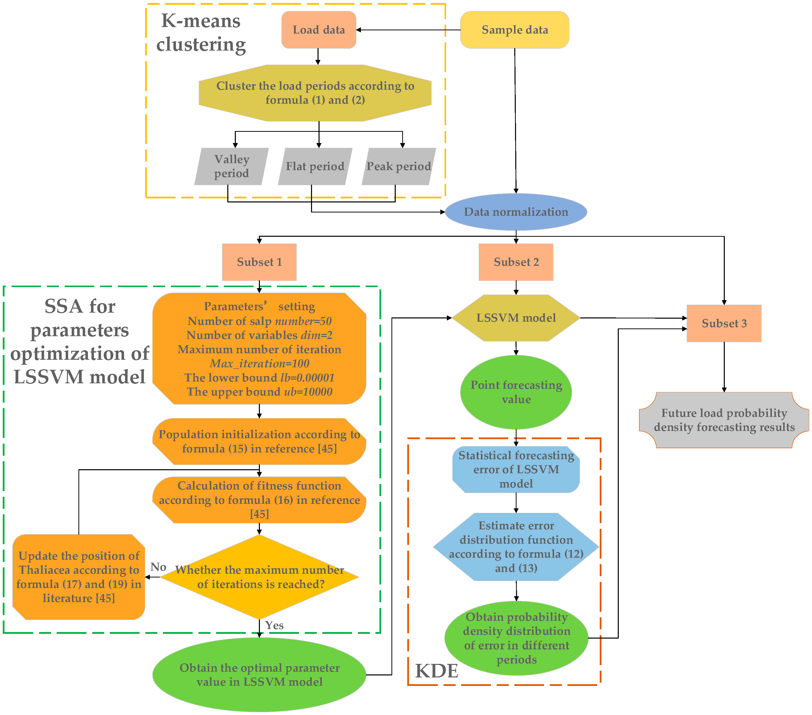
4. The Framework of the Proposed Method

On the basis of the idea of “point forecasting plus kernel density estimation”, this paper put forward a hybrid load forecasting model, which combines K-means clustering method, LSSVM, SSA algorithm, and kernel density estimation. The specific calculation process of the model is as follows.

Step 1 Data preprocessing

Collect and sort out the meteorological data such as temperature, humidity, and wind speed at 24 h of the day. Standardize the load data and influencing factor data, converting their values to [1]. Then, use the meteorological data and the load data of the first two days of the day to be forecasted as input variables and use the load of the day to be predicted as output variables to build the sample set. The sample set is divided into three subsets: subset 1 is used to train the model, subset 2 is used to calculate the prediction error and estimate the error distribution, and the performance of the model is verified by subset 3.

Step 2 K-means clustering

For the load data, K-means clustering algorithm is adopted to aggregate the load data of 24 h of a day into three types. Each type corresponds to three periods, that is, valley period, flat period, and peak period.

Step 3 Parameters setting

Five parameters need to be set before the start of SSA iteration processing, including number of salp number, number of variables dim, maximum number of iteration Max_iteration, lower bound lb, and upper bound ub. We set that number = 50, dim = 2, Max_iteration = 100, lb = 0.00001, and ub = 10,000.

Training samples and test samples were used to conduct point forecasting of load at 24 time points through the LSSVM model. During this process, two parameters of gamma and sigma ^2 in LSSVM model were optimized by SSA optimization algorithm.

Step 4 Point forecasting

The samples in subset 1 are input into the SSA, and the optimal parameter values of the LSSVM are obtained through multiple iterations. Then, the sample data in subset 2 is input into the trained model to obtain the point forecasting value of the load at each hour.

Step 5 Estimation of error distribution

According to the statistics of the point forecasting error data of valley period, flat period, and peak period obtained in the previous step, the probability density function of error distribution for each period is estimated by using the kernel density estimation method, and then the probability density function of forecasting error distribution for each time point in 24 time points of a day is obtained.

Step 6 Calculation of probability density prediction results

The sample data in subset 3 was taken as the samples to be predicted and input into the trained SSA-LSSVM model to obtain the point predicted value. Combined with the error distribution results in step 5, the probability density forecasting results of loads at each moment are obtained, and then the upper and lower limits of the confidence interval under the given signal level are solved. At this time, the load probability density forecasting is completed.

In this paper, the forecasting effect of the model is mainly evaluated from two aspects: interval coverage and interval average width [46,47,48].

(1) Interval coverage

The interval coverage ${\delta }_{PICP}$ is used to express the probability of the predicted interval covering the real value. The larger the value is, the better the forecasting effect is. The calculation formula is as follows.

$${\delta }_{PICP}=\frac{1}{N}{\displaystyle \sum }_{i=1}^N{c}_i$$

(15)

where N represents the number of samples, and $c_i$ is the variable. For each sample point, if the real value falls within the forecasting interval, then $c_i=1$, otherwise $c_i=0$.

(2) Average width of interval

The interval average width $W_A$ is used to measure the validity of the forecasting interval width. The larger the value is, the greater the interval width is, and the worse the forecasting performance is. The calculation formula is as follows.

$$W_A=\frac{1}{N}{\displaystyle \sum }_{i=1}^N{w}_i$$

(16)

where $w_i$ is the forecasting interval width of the i-th sample.

The procedure of the proposed hybrid model for hourly power load forecasting is illustrated in Figure 1.

5. Empirical Results and Analysis

This paper constructs a probability density forecasting model based on K-means clustering, SSA-LSSVM and kernel density estimation. To illustrate the forecasting process and verify the validity of the proposed model, based on the actual sample data, this paper solves the probability density forecasting results according to the process in Section 4, and verifies the effect of the model through the above evaluation indexes. In addition, by setting up the contrast model, the practicability and validity of the model are further explained.

5.1. Data Sorting and Preprocessing

In this paper, 85 days of data from a city in northern China from 1 September to 24 November 2018 are used for empirical analysis, and the sample set is divided into three subsets. Subset 1 is the training sample, which contains 1224 h of data from September 1 to October 21. Subset 2 is the test sample with 624 h of data from October 22 to November 16. Subset 3, including 192 h data from 17 November to 24 November, is the sample to be forecasted. In consideration of the difference of load fluctuations between holidays and non-holidays, this paper clusters and forecasts the holidays and non-holiday loads, respectively. The data set includes hourly load, temperature, humidity, wind speed, air pressure, precipitation, and air quality. In consideration of the influence of historical load on the daily load to be predicted, the load value of the same time point on the first two days of the date to be predicted is taken into account as the influencing factor during model training and forecasting. The descriptive statistics of all indicators are shown in

Table 1. Descriptive statistics of sample data.

	Unit	N	Max.	Min.	Mean	S.D.
Load	GW	2040	163.9060	61.4797	112.0106	23.5318
Temperature	°C	2040	33.1	−3.7	14.2171	7.5424
Humidity	g/m3	2040	97	11	50.9137	23.6818
Wind speed	m/s	2040	8.6	0	1.8655	1.3130
Air pressure	kPa	2040	1030.8	995.5	1015.8346	6.3951
Rainfall	mm	2040	3.6	0	0.0153	0.1819
Air quality level	/	2040	310	9	61.1656	51.2375

.

Before the forecasting, the raw data needs to be normalized to eliminate the influence of the dimensional difference between the indicator values on the final forecasting result. The standardized processing calculation formula is as follows.

$$x_{ij}^{\prime }=\frac{x_{ij}-x_{minj}}{x_{maxj}-x_{minj}}$$

(17)

where $x_{ij}$ represents the original data of the j-th data of the i-th indicator, and $x_{ij}^{\prime }$ represents the processed data. $x_{minj}=\underset{i}{\min }{x}_{ij}$, $x_{maxj}=\underset{i}{\max }{x}_{ij}$, $\mathrm{i}=1,2,\dots ,7$.

The descriptive statistical values of the normalized data are shown in

Table 2. Descriptive statistics for normalized sample data.

	N	Max.	Min.	Mean	S.D.
Load	2040	1	0	0.4933	0.2297
Temperature	2040	1	0	0.4869	0.2050
Humidity	2040	1	0	0.4641	0.2754
Wind speed	2040	1	0	0.2169	0.1527
Air pressure	2040	1	0	0.5761	0.1812
Rainfall	2040	1	0	0.0043	0.0505
Air quality level	2040	1	0	0.1733	0.1702

.

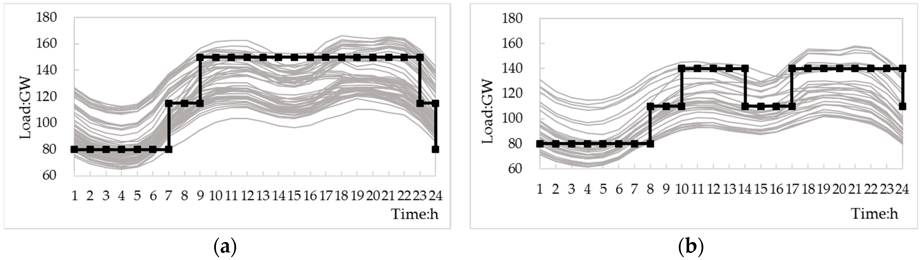
5.2. K-Means Clustering Results

In this paper, the K-means clustering algorithm is used to aggregate the load data at 24 h in the day into the valley period, the flat period, and the peak period; the load clustering results of holidays and non-holidays are shown in Figure 2.

For holidays and non-holidays, there are significant differences in the time points corresponding to the valley period, the flat period, and the peak period in the clustering results, indicating that holidays present a certain degree of influence on the load. In addition, during the period from 10:00 to 13:00, the non-holiday load has a clear upward trend compared with the holiday load. Therefore, to avoid the influence of a single model on the distribution density estimation of the error, this paper considers the forecasting of holiday and non-holiday load separately.

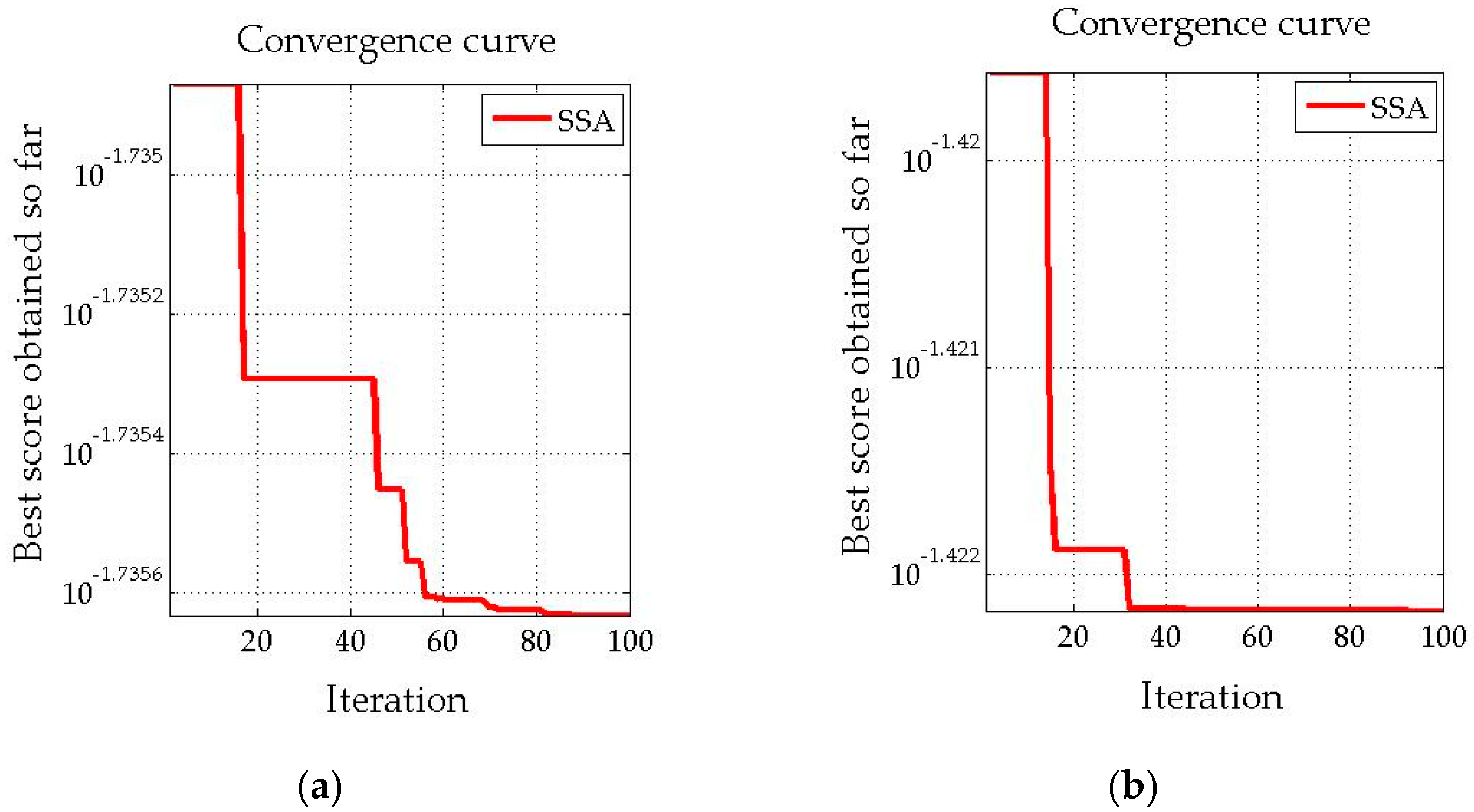
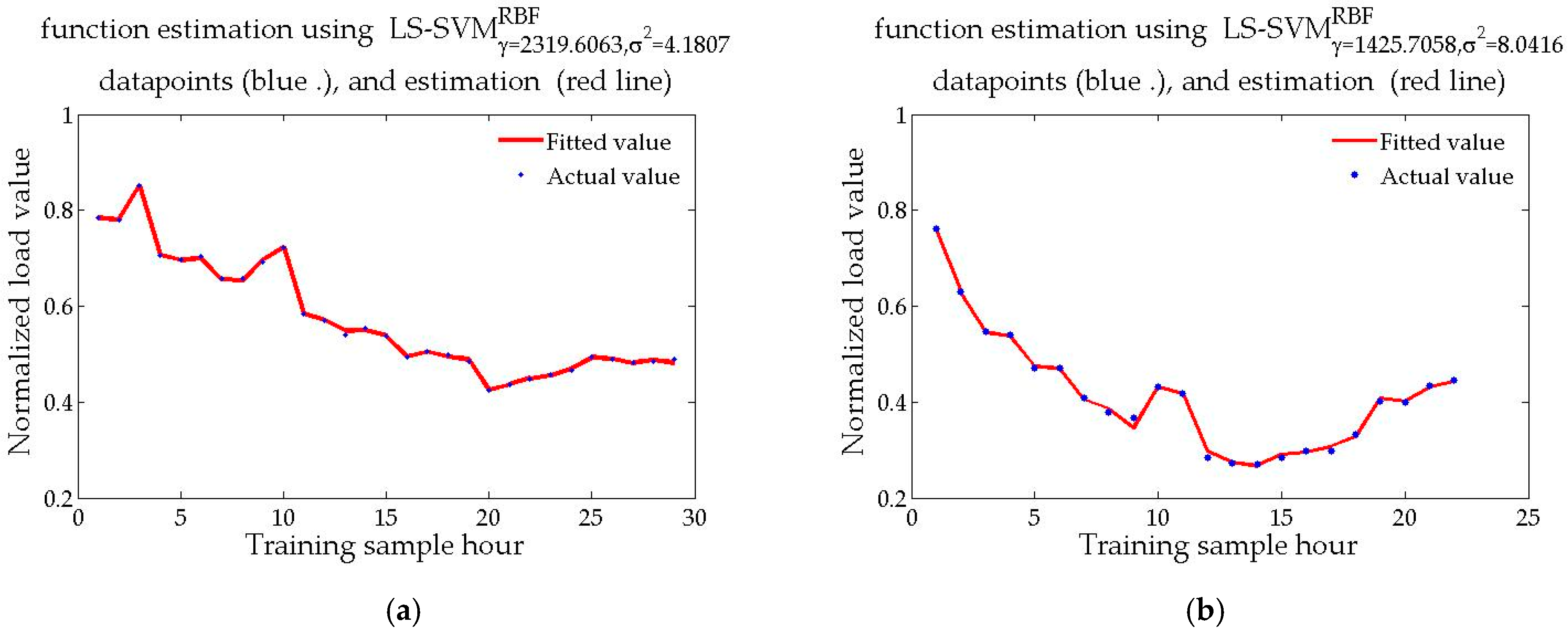
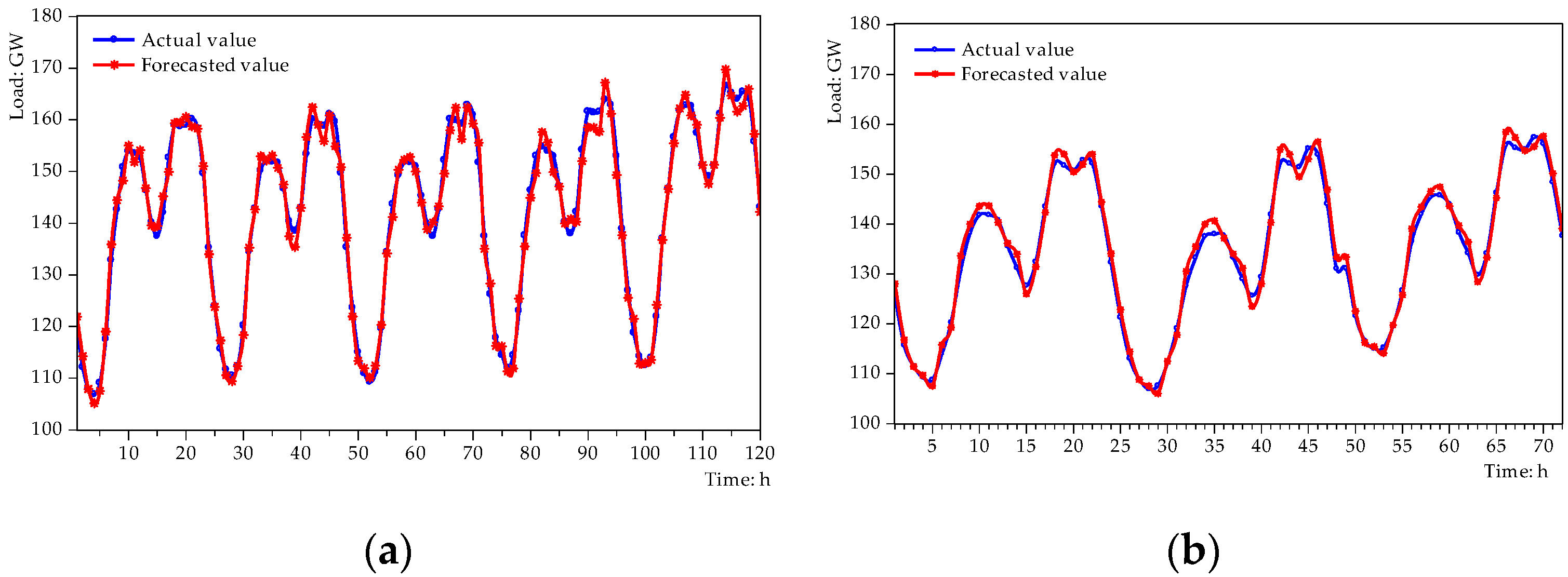
5.3. SSA-LSSVM Forecasting Results

In this paper, the SSA-LSSVM model is used to predict the point of load forecasting. Before the forecasting, the model is trained by the training sample to fit the relationship between the load and the influencing factors. In this process, the γ and ${\sigma }^2$ parameters in the LSSVM model are optimized by the SSA algorithm to improve the forecasting performance of the model. The training and forecasting process was done using MATALB 2014a. The following describes the optimization process at 13:00. The parameters of LSSVM optimized by SSA are as follows. For non-holidays, $\gamma =1019.6063$, ${\sigma }^2=5.1807$, and the fitness function value of SSA-LSSVM model is 0.0184, that is, the model fitting accuracy can reach over 98%. For holidays, $\gamma =1425.7058$, ${\sigma }^2=8.0416$, and the fitness function value of the SSA-LSSVM model is 0.0201, which means the model fitting accuracy can reach over 97%. The process of parameter optimization is shown in Figure 3.

The parameters optimized by the SSA algorithm are imported into the LSSVM model, and the optimized model fitting effect is shown in Figure 4.

The trained model is used to forecast the load at each time in subset 3, and then the forecasted value of each time is obtained. The SSA-LSSVM model forecasting result can be obtained by comparing the predicted results at each time with the actual values, as shown in Figure 5.

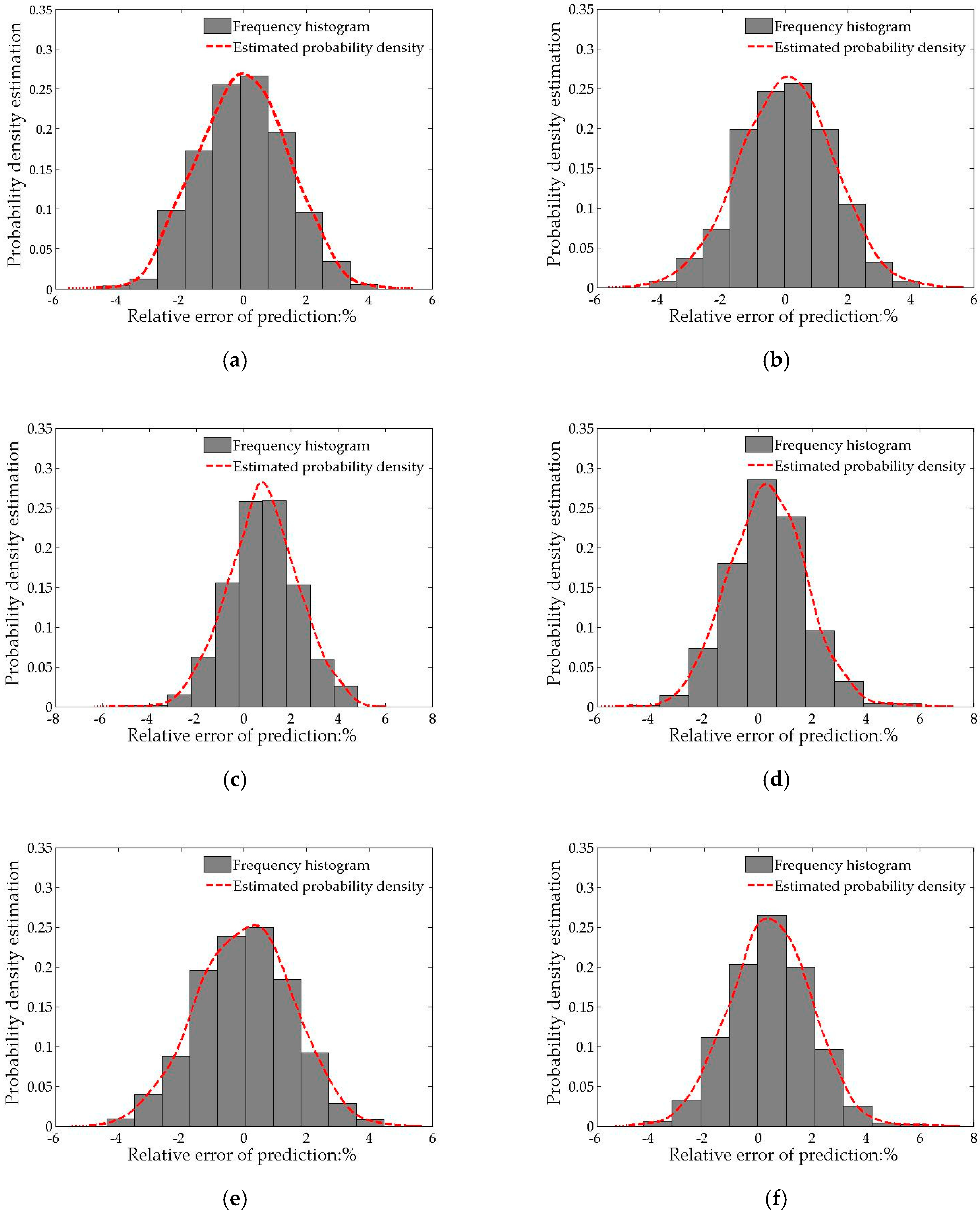
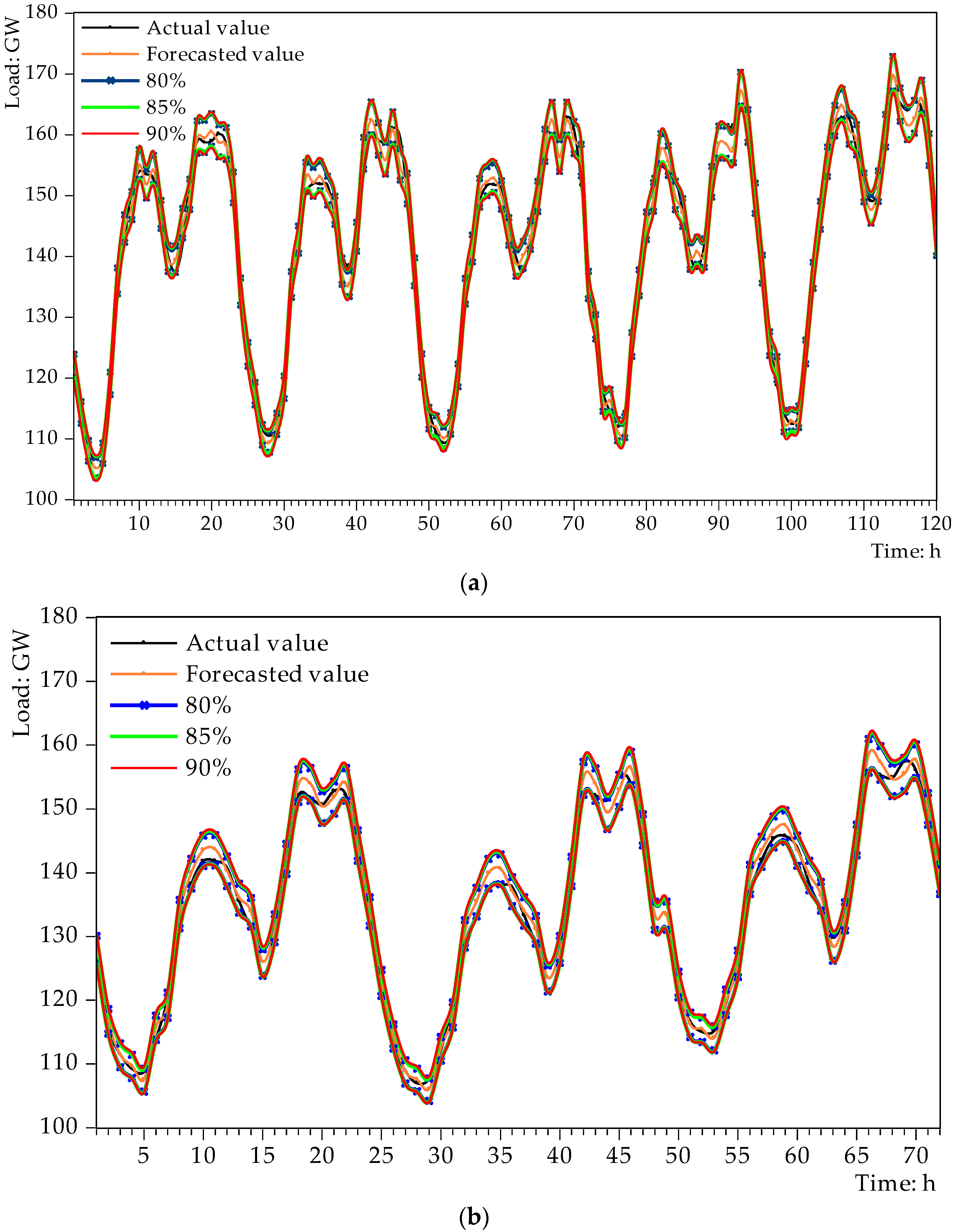
5.4. Probability Density Forecasting Results

Applying the formula (12) to estimate the kernel density of the load point forecasting error in the subset 2, the error distribution histogram and the error distribution probability density curve of valley periods, the flat period, and the peak period of non-holidays and holidays can be obtained respectively, as shown in Figure 6.

5.5. Results and Discussion

In combination with the load point forecasting results and the forecasting error distribution, the distribution of load at each moment can be further calculated. By giving a certain confidence level, the load forecasting confidence interval at this confidence level can be solved. Furthermore, by calculating and comparing the predicted evaluation index values at different confidence levels by Equations (15) and (16), the probability density forecasting performance of the model can be analyzed. The specific results are shown in Figure 7 and

Table 3. Probability density forecasting effect of the model proposed in this paper.

Confidence Level/%	${\mathit{\delta }}_{\mathit{P}\mathit{I}\mathit{C}\mathit{P}}/\%$		${\mathit{W}}_{\mathit{A}}/\mathbf{Gigawatt}\left(\mathbf{GW}\right)$
	Non-Holidays	Holidays	Non-Holidays	Holidays
80	93.33	90.28	3.5597	4.0156
85	96.67	95.83	3.812	4.2932
90	100	98.61	4.7921	5.4212

.

In this paper, a load forecasting model based on K-means clustering, SSA-LSSVM method, and Gaussian kernel density estimation is proposed. To verify the validity of the proposed model, the following models are selected as comparisons.

Model 1: The load forecasting model based on K-means clustering analysis, SSA-LSSVM method, and Gaussian kernel density estimation in this paper;

Model 2: Load forecasting model based on K-means clustering analysis, LSSVM model method, and kernel density estimation, which does not consider the improvement of LSSVM method by SSA optimization algorithm;

Model 3: Load forecasting model based on K-means clustering analysis, SSA-LSSVM method, and parameter estimation, in which the assumed error in the parameter estimation obeys the β distribution;

Model 4: Load forecasting model based on K-means clustering analysis, SSA-LSSVM method, and kernel density estimation, in which the kernel function adopts triangular kernel function.

Using the same sample data, the above four models are used to separately predict the probability density, and then the forecasting performance of the model is evaluated using Equations (15) and (16), as shown in

Table 4. Comparison of model forecasting effects.

Model	Confidence Level/%	${\mathit{\delta }}_{\mathit{P}\mathit{I}\mathit{C}\mathit{P}}/\%$		${\mathit{W}}_{\mathit{A}}/\mathbf{GW}$
		Non-Holidays	Holidays	Non-Holidays	Holidays
Model 1	80	93.33	90.28	3.5597	4.0156
	85	96.67	95.83	3.812	4.2932
	90	100	98.61	4.7921	5.4212
Model 2	80	88.33	86.11	3.7352	4.4373
	85	94.17	91.67	4.0689	4.7481
	90	95.83	93.06	4.9857	5.8837
Model 3	80	87.5	83.33	4.7498	4.9215
	85	91.67	86.11	4.7838	4.9375
	90	95.83	90.28	5.5247	6.0786
Model 4	80	95.83	90.28	3.5172	3.8225
	85	95.83	94.44	3.9034	4.6896
	90	100	98.61	4.7943	5.6759

.

The following findings can be concluded from Table 4:

(1).

By comparing model 1 and model 2, it can be found that the model optimized by SSA algorithm can significantly improve the interval coverage and reduce the interval average width. This is because the optimized model can effectively find the parameter values in the LSSVM model, avoiding the subjectivity of artificially given parameters, and thus improving the model forecasting performance.

(2).

By comparing model 1 and model 3, it can be found that, in comparison with the traditional parameter estimation, the non-parametric estimation method can effectively improve the interval coverage and reduce the interval average width. This is because the traditional parameter estimation method needs to make assumptions about the probability density function in advance when estimating the error distribution of point forecasting. In contrast, the non-parametric estimation method can better reflect the true distribution of the error, and the fitting effect is better.

(3).

By comparing model 1 and model 4, it can be found that the two models perform similarly on the interval coverage and interval average width. On the interval average width index, model 1 is slightly better than model 4, but the difference is not obvious, indicating that the selection of the kernel function does not show a greater difference in the improvement of the model forecasting performance relative to the improvement of other parts of the model.

6. Conclusions

With the acceleration of the power market reform process, the importance of short-term load forecasting for grid companies and emerging purchase and sale companies is becoming more apparent. At the same time, affected by many uncertain factors, the future load changes present uncertainty. In comparison with the traditional point forecasting method, the probability density forecasting can reflect more uncertain information of future load fluctuation, which is more conducive to the decision-making and execution of electricity purchase and sale strategies of each power trading subject, and further promote the economics of electricity market trading.

Accordingly, this paper proposes a load probability density forecasting model based on K-means clustering, SSA-LSSVM, and kernel density estimation. This paper applies the idea of “point forecasting plus error probability density estimation”. Firstly, K-means clustering algorithm was used to divide the load at 24 h of a day into different periods of peak, flat, and valley. Secondly, SSA-LSSVM method was used to obtain the load point forecasting results at the next 24 moments, and the forecasting errors at different time periods were statistically calculated. The probability density function of load forecasting errors at different time periods was fitted with the kernel density estimation method to obtain the error distribution. Finally, given the confidence level, the load confidence interval can be further solved from the point predicted value and error distribution. The validity of the proposed model is verified by comparing it with several other models.

This paper aims at the short-term load forecasting in the next few hours, and the span of data samples is small, so the forecasting results will not be affected by seasonal changes. Therefore, the model in this paper can be applied to short-term load forecasting in all periods of the year, but the process of sample set construction may be slightly different due to different seasons. Although the model proposed in this paper needs a complicated calculation process, the results show that the model can effectively improve the load forecasting performance; it can provide reasonable support for the economic operation of power system. Meanwhile, the proposed model can be further combined with other intelligent optimization algorithms to improve the forecasting performance of the model. In addition, the clustering algorithm can be further improved, and on this basis, the model can be applied to the load forecasting of renewable energy power generation side and micro-grid, etc.

References

1. Qi, L.; Zhen, H.; Sheng, L. Research on power load forecasting based on support vector machine. J. Balk. Tribol. Assoc. 2016, 22, 151–159. [Google Scholar]
2. Zhang, Q.; Lu, J.; Yang, Z.; Tu, M. A Deep Learning Based Real-time Load Forecasting Method in Electricity Spot Market. J. Phys. Conf. Ser. 2019, 1176, 062068. [Google Scholar] [CrossRef]
3. Yan, Q.; Qin, C.; Nie, M.; Yang, L. Forecasting the electricity demand and market shares in retail electricity market based on system dynamics and Markov chain. Math. Probl. Eng. 2018, 1–11. [Google Scholar] [CrossRef]
4. Li, W.; Quan, C.; Wang, X.; Zhang, S. Short-term power load forecasting based on a combination of VMD and ELM. Pol. J. Environ. Stud. 2018, 27, 2143–2154. [Google Scholar] [CrossRef]
5. Li, Z.; Yin, X.; Yang, H.; Ma, R.; Shi, G.; Zhao, W. Analysis of seasonal load characteristics based on improved k-means clustering algorithm. Grid Clean Energy 2018, 34, 53–59+64. [Google Scholar]
6. Kang, Y.; Yin, S.; Wang, X.; Dong, S.; Deng, X.; Chen, G. Analysis of load characteristics and influencing factors of large urban power grid. Electr. Meas. Instrum. 2016, 53, 51–56. [Google Scholar]
7. Li, J.; Sang, C.; Gan, Y.; Pan, Y. Research overview of wind power prediction technology. Mod. Electr. Power 2017, 34, 1–11. [Google Scholar]
8. Goodwin, P.; Önkal, D.; Thomson, M. Do forecasts expressed as prediction intervals improve production planning decisions? Eur. J. Op. Res. 2010, 205, 195–201. [Google Scholar] [CrossRef]
9. Zhang, Y.; Wang, J.; Wang, X. Review on probabilistic forecasting of wind power generation. Renew. Sustain. Energy Rev. 2014, 32, 255–270. [Google Scholar] [CrossRef]
10. Van der Meer, D.W.; Widén, J.; Munkhammar, J. Review on probabilistic forecasting of photovoltaic power production and electricity consumption. Renew. Sustain. Energy Rev. 2018, 81, 1484–1512. [Google Scholar] [CrossRef]
11. Yu, X. Research on Ultra-Short-Term Load Forecasting of Micro Power Grid. Master’s Thesis, Jiangnan University, Jiangsu, China, June 2018. [Google Scholar]
12. Hernández, J.C.; Ruiz-Rodriguez, F.J.; Jurado, F. Modelling and assessment of the combined technical impact of electric vehicles and photovoltaic generation in radial distribution systems. Energy 2017, 141, 316–332. [Google Scholar] [CrossRef]
13. Pinson, P.; Tastu, J. Discussion of “Prediction intervals for short-term wind farm generation forecasts” and “Combined nonparametric prediction intervals for wind power generation”. IEEE Trans. Sustain. Energy 2014, 5, 1019–1020. [Google Scholar] [CrossRef] [Green Version]
14. Guan, C.; Luh, P.B.; Michel, L.D.; Chi, Z.Y. Hybrid Kalman filters for very short-term load forecasting and prediction interval estimation. IEEE Trans. Power Syst. 2013, 28, 3806–3817. [Google Scholar] [CrossRef]
15. Quan, H.; Srinivasan, D.; Khosravi, A. Uncertainty handling using neural network-based prediction intervals for electrical load forecasting. Energy 2014, 73, 916–925. [Google Scholar] [CrossRef]
16. Li, Z.; Ding, J.; Wu, D.; Wen, F. Integrated limit learning machine method for power load interval prediction. J. North China Electr. Power Univ. Nat. Sci. Ed. 2014, 41, 78–88. [Google Scholar]
17. Yu, J.; Bao, Z.; Li, Z. User load interval prediction method based on LSTM. Ind. Control Comput. 2018, 31, 100–102. [Google Scholar]
18. Ren, J.; Zhang, L.; Wang, H.; Guo, Q. Prediction of short-term load interval based on IPSO-GPR. Comput. Eng. Des. 2019, 40, 3002–3008. [Google Scholar]
19. Meng, Y. Study on Short-Term Load Probability Density Prediction Method Based on Regression Analysis. Master’s Thesis, North China Electric Power University (Beijing), Beijing, China, June 2018. [Google Scholar]
20. Liu, R. Prediction Method of Short-Term Power Load Probability Density Based on Support Vector Quantile Regression and Smart Grid. Master’s Thesis, Hefei University of Technology, Anhui, China, June 2017. [Google Scholar]
21. Nowotarski, J.; Weron, R. Recent advances in electricity price forecasting: A review of probabilistic forecasting. Renew. Sustain. Energy Rev. 2018, 81, 1548–1568. [Google Scholar] [CrossRef]
22. Chen, L. Short-Term Load Prediction and Confidence Interval Based on Non-Linear Ensemble. Master’s Thesis, Tianjin University, Tianjin, China, June 2016. [Google Scholar]
23. Wen, C. Study on Probability Density Prediction Method Based on Neural Network Quantile Regression and Kernel Density Estimation. Master’s Thesis, Hefei University of Technology, Anhui, China, June 2015. [Google Scholar]
24. Bracale, A.; Carpinelli, G.; De Falco, P. A Bayesian-based approach for the short-term forecasting of electrical loads in smart grids. Part I: Theoretical aspects. In Proceedings of the 2016 International Symposium on Power Electronics, Electrical Drives, Automation and Motion (SPEEDAM), Anacapri, Italy, 22–24 June 2016. [Google Scholar]
25. Bikcora, C.; Verheijen, L.; Weiland, S. Density forecasting of daily electricity demand with ARMA-GARCH, CAViaR, and CARE econometric models. Sustain. Energy Grids Netw. 2018, 13, 148–156. [Google Scholar] [CrossRef]
26. Jiang, Y.; Huang, G. Short-term wind speed prediction: Hybrid of ensemble empirical mode decomposition, feature selection and error correction. Energy Convers. Manag. 2017, 144, 340–350. [Google Scholar] [CrossRef]
27. Guo, R. Selection of Conditional Heteroscedasticity Model Based on Density Prediction. Master’s Thesis, Shandong University, Shandong, China, June 2012. [Google Scholar]
28. Sun, Z. Analysis and Research on Gas Load Characteristics and Gas Consumption Characteristics of Commercial Users in Chongqing. Master’s Thesis, Chongqing University, Chongqing, China, June 2017. [Google Scholar]
29. He, Y.; Liu, R.; Li, H.; Wang, S.; Lu, X. Short-term power load probability density forecasting method using kernel-based support vector quantile regression and Copula theory. Appl. Energy 2017, 185, 254–266. [Google Scholar] [CrossRef] [Green Version]
30. Yang, Y.; Li, S.; Li, W.; Qu, M. Power load probability density forecasting using Gaussian process quantile regression. Appl. Energy 2018, 213, 499–509. [Google Scholar] [CrossRef]
31. He, Y.; Xu, Q.; Wan, J.; Yang, S. Short-term power load probability density forecasting based on quantile regression neural network and triangle kernel function. Energy 2016, 114, 498–512. [Google Scholar] [CrossRef]
32. He, Y.; Wen, C.; Xu, Q. Probability density prediction method of medium power load based on Epanechnikov kernel and optimal window width combination. Power Autom. Equip. 2016, 36, 120–126. [Google Scholar]
33. He, Y.; Qin, Y.; Lei, X.; Feng, N. A study on short-term power load probability density forecasting considering wind power effects. Int. J. Electr. Power Energy Syst. 2019, 113, 502–514. [Google Scholar] [CrossRef]
34. Sanchez-Sutil, F.; Cano-Ortega, A.; Hernandez, J.C.; Rus-Casas, C. Development and calibration of an open source, low-cost power smart meter prototype for PV household-prosumers. Electronics 2019, 8, 878. [Google Scholar] [CrossRef] [Green Version]
35. Li, N.; Wang, L.; Zhang, W.; Wang, Y.; Shu, Y.; Zhang, C. Study on long period peak/valley division model based on high-dimensional data optimization clustering. Mod. Electr. Power 2016, 33, 67–71. [Google Scholar]
36. Suykens, J.A.K.; Lukas, L.; Vandewalle, J. Sparse approximation using least squares support vector machines. In Proceedings of the 2000 IEEE International Symposium on Circuits and Systems. Emerging Technologies for the 21st Century. Proceedings (IEEE Cat No. 00CH36353), Dalian, China, 26–28 July 2017; Volume 2, pp. 757–760. [Google Scholar]
37. Wang, H.; Hu, D. Comparison of SVM and LS-SVM for regression. In Proceedings of the 2005 International Conference on Neural Networks and Brain, Beijing, China, 13–15 October 2015; Volume 1, pp. 279–283. [Google Scholar]
38. Adankon, M.M.; Cheriet, M. Model selection for the LS-SVM. Application to handwriting recognition. Pattern Recognit. 2009, 42, 3264–3270. [Google Scholar] [CrossRef] [Green Version]
39. Deo, R.C.; Tiwari, M.K.; Adamowski, J.F.; Quilty, J.M. Forecasting effective drought index using a wavelet extreme learning machine (W-ELM) model. Stoch. Environ. Res. Risk Assess. 2017, 31, 1211–1240. [Google Scholar] [CrossRef]
40. Zhao, H.; Zhao, H.; Guo, S. Short-term wind electric power forecasting using a novel multi-stage intelligent algorithm. Sustainability 2018, 10, 881. [Google Scholar] [CrossRef] [Green Version]
41. Mirjalili, S.; Gandomi, A.H.; Mirjalili, S.Z.; Saremi, S.; Faris, H.; Mirjalili, S.M. Salp Swarm Algorithm: A bio-inspired optimizer for engineering design problems. Adv. Eng. Softw. 2017, 114, 163–191. [Google Scholar] [CrossRef]
42. Li, X.; Li, B.; Zhao, L.; Zhao, H.; Xue, W.; Guo, S. Forecasting the short-term electric load considering the influence of air pollution prevention and control policy via a hybrid model. Sustainability 2019, 11, 2983. [Google Scholar] [CrossRef] [Green Version]
43. Jafarizadeh, M.A.; Fouladi, N.; Sabri, H.; Maleki, B.R. A non-parametric estimation approach in the investigation of spectral statistics. Indian J. Phys. 2013, 87, 919–927. [Google Scholar] [CrossRef]
44. Han, Q.; Ma, S.; Wang, T.; Chu, F. Kernel density estimation model for wind speed probability distribution with applicability to wind energy assessment in China. Renew. Sustain. Energy Rev. 2019, 115, 109387. [Google Scholar] [CrossRef]
45. Yang, N.; Zhou, Z.; Chen, D.; Wang, X.; Li, H.; Li, S. Wind power fluctuation probability density modeling method based on non-parametric kernel density estimation. J. Sol. Energy 2019, 40, 2028–2035. [Google Scholar]
46. Liu, C.; Cao, W.; Wang, Z. Short-term interval prediction of wind power based on fuzzy c-means soft cluster condition identification. J. North China Electr. Power Univ. Nat. Sci. Ed. 2019, 46, 83–91. [Google Scholar]
47. Li, M.; Lin, X.; Zhang, Z.; Weng, H. Prediction algorithm of ultra-short-term pv output interval and its application. Power Syst. Autom. 2019, 43, 10–18. [Google Scholar]
48. Yang, X.; Ma, X.; Kang, N.; Maihemuti, M. Probability interval prediction of wind power based on KDE method with rough sets and weighted Markov chain. IEEE Access 2018, 6, 51556–51565. [Google Scholar] [CrossRef]
Figure 1. The procedure of the proposed hybrid model for hourly power load forecasting. SSA: Salp swarm algorithm; KDE: kernel density estimation.
Sustainability 11 06954 g001
Figure 2. K-means clustering results. (a) Non-holiday peak-to-valley time division results. (b) Holiday peak-to-valley time division results.
Sustainability 11 06954 g002
Figure 3. The process of parameter optimization. (a) The process of iterative optimization at 13:00 on non-holidays. (b)The process of iterative optimization at 13:00 on holidays.
Sustainability 11 06954 g003
Figure 4. Salp Swarm Algorithm (SSA)-Least Square Support Vector Machine (LSSVM) model fitting effect. (a) SSA-LSSVM Model fitting effect at 13:00 on non-holidays. (b) SSA-LSSVM Model fitting effect at 13 o’clock on holidays.
Sustainability 11 06954 g004
Figure 5. Load point forecasting results of the day in subset 3. (a) Results of the load point forecast for non-holidays. (b) Results of the load point forecast for holidays.
Sustainability 11 06954 g005
Figure 6. Error fitting results in different time periods. (a) The valley period of non-holidays. (b) The valley period of holidays. (c) The flat period of non-holidays. (d) The flat period of holidays. (e) The peak period of non-holidays. (f) The peak period of holidays.
Sustainability 11 06954 g006
Figure 7. Load forecast results at different confidence levels. (a) Forecasting results for non-holidays. (b) Forecasting results for holidays.
Sustainability 11 06954 g007