Intelligent Prediction of Minimum Miscibility Pressure (MMP) During CO₂ Flooding Using Artificial Intelligence Techniques

Abstract

Carbon dioxide (CO₂) injection is one of the most effective methods for improving hydrocarbon recovery. The minimum miscibility pressure (MMP) has a great effect on the performance of CO₂ flooding. Several methods are used to determine the MMP, including slim tube tests, analytical models and empirical correlations. However, the experimental measurements are costly and time-consuming, and the mathematical models might lead to significant estimation errors. This paper presents a new approach for determining the MMP during CO₂ flooding using artificial intelligent (AI) methods. In this work, reliable models are developed for calculating the minimum miscibility pressure of carbon dioxide (CO₂-MMP). Actual field data were collected; 105 case studies of CO₂ flooding in anisotropic and heterogeneous reservoirs were used to build and evaluate the developed models. The CO₂-MMP is determined based on the hydrocarbon compositions, reservoir conditions and the volume of injected CO₂. An artificial neural network, radial basis function, generalized neural network and fuzzy logic system were used to predict the CO₂-MMP. The models’ reliability was compared with common determination methods; the developed models outperform the current CO₂-MMP methods. The presented models showed a very acceptable performance: the absolute error was 6.6% and the correlation coefficient was 0.98. The developed models can minimize the time and cost of determining the CO₂-MMP. Ultimately, this work will improve the design of CO₂ flooding operations by providing a reliable value for the CO₂-MMP.

1. Introduction

Enhanced oil recovery (EOR) processes are used to create favorable conditions for producing oil, through interfacial tension (IFT) reduction, wettability alteration or decreasing the oil viscosity [1]. CO₂ injection is one of the most practical and effective EOR methods because it significantly reduces the oil viscosity and improves the sweep efficiency [2,3]. The minimum miscibility pressure (MMP) plays a significant role in designing the gas flooding operations. The minimum miscibility pressure can be measured using slim tube tests [4]. However, the laboratory measurements are costly and time-consuming [5]. MMP can also be determined using empirical correlations, but these correlations can lead to significant deviations, where the absolute error can reach up to 25% [6,7,8,9,10]. Several empirical correlations were proposed to estimate the MMP based on the reservoir condition and the fluids compositions. The empirical correlations were developed utilizing regression approaches. The common correlations are the Glaso correlation, Sebastian et al. correlation and Khazam et al. correlation [6,8,9]. Generally, the accuracy of the empirical correlations is increasing as the mathematical complexity of the equation increases. Most of the empirical correlations are used mainly for the fast screening applications [10].

In addition, analytical methods have been coupled with the equation of state (EOS) to estimate the MMP, and an average absolute percentage error of 15.7% is reported. The main advantage of analytical methods is that they can determine the MMP without introducing uncertainties associated with the condensing or vaporizing displacement (CV) process. Since the displacement processes are associated with complex miscibility mechanisms and then reduce the reliability of MMP prediction [11,12,13], Yuan et al. [14,15] applied the analytical gas theory to estimate the CO₂-MMP. They used more than 180 data sets to build and evaluate the proposed semi-empirical model. They concluded that the developed model is more accurate and reliable than the empirical correlations, with a maximum average absolute percentage error of 9%. Furthermore, numerical approaches are used to determine the MMP. Fine-grid compositional simulations are utilized to solve the equation of state for particular grid sizes. The advantage of this approach is that it can be applied for heterogenous system of different pressure and temperature distributions as well as various fluid compositions. However, the numerical models can suffer from stability problems and may require a significantly small time-step in order to obtain stable solutions [10,15].

The use of artificial intelligence (AI) has proved to be an effective tool for prediction tasks because AI can capture the complex relationships between the output and input parameters [16]. Artificial neural network (ANN) is the most famous technique applied in the petroleum industry [17,18,19,20]. ANN technique has been utilized to predict the drilling fluids rheology, estimate the reservoir permeability and characterize the unconventional reservoirs [21,22,23,24,25,26]. AI also has been used for predicting the performance of several enhanced oil recovery (EOR) processes, such as steam-assisted gravity drainage (SAGD) process in heavy oil reservoirs [27,28,29].

Edalat et al. [30] presented a new ANN model to determine the MMP during hydrocarbon injection operations. Multi-layer perceptron (MLP) with two-layer feed-forward backpropagation were used. A total of 52 data points from an Iranian oil reservoir was employed with 20% for testing and 80% for training. They compared their results with a slim tube test and correlations, the maximum error of 18.58% and R-squared (R²) of 0.938 is reported. They concluded that their ANN model can determine the MMP for different fluid compositions.

Dehghani et al. [31] combined a genetic algorithm with an ANN technique (GA–ANN) to determine the minimum miscibility pressure for gas injection operations. A total of 46 data points of MMP experiments were utilized, and back propagation with two hidden layers was used. The GA–ANN model predicts the MMP using the reservoir parameters and the injected-gas composition. They concluded that the developed model can afford a high level of dependability and accuracy for determining the MMP.

Shokrollahi et al. [32] utilized a support vector machine technique to determine the MMP for CO₂-injection operations. A total of 147 data points from experimental CO₂-MMP was used to developed and validate the model reliability, and the values of coefficient of determination (R²) and average absolute percentage error were 0.90% and 9.6%, respectively. They mentioned that the proposed model shows high performance and good matching with the experimental data.

Liu et al. [33] suggested an improved method for estimating the CO₂-MMP utilizing magnetic resonance imaging (MRI). The obtained results showed good agreements with the experimental measurements. Khazam et al. [9] developed a simple correlation to determine the CO₂-MMP using a regression tool. A total of 100 PVT measurements from Libyan oilfields were used with a wide range of conditions, and a CO₂-MMP between 1544 and 6244 psia. The developed correlation requires the values of the oil properties and system condition (pressure and temperature) to estimate the CO₂-MMP with a high degree of accuracy, R² is 0.95 and AAPE is 5.74%. However, the model was developed based on limited data and from one region, and all samples were collected from Libyan oilfields. Czarnota et al. [5] presented a new approach to estimate the CO₂-MMP using an acoustic separator by taking images for the CO₂/oil system as a function of system pressure. They mentioned that the proposed approach can minimize the time required to obtain the CO₂-MMP.

Rostami et al. [34] applied the support vector machine (SVM) technique to estimate the CO₂-MMP during CO₂ flooding. SVM was used to determine the CO₂-MMP for live and dead crude oil systems. The developed model showed an accurate prediction with the average absolute relative deviation (AARD) of less than 3% and minimum coefficient of determination (R²) of 0.99. However, no direct equation is reported and the developed SVM model is considered as a black box model. Alfarge et al. [35] used laboratory measurements and field studies to characterize the CO₂-flooding in shale reservoirs; more than 95 case studies were used. They constructed a proxy system to predict the incremental oil recovery based on the affecting parameters. The relationship between rock properties and incremental oil recovery were explained; the effect of permeability, porosity, total organic carbon content and fluid saturations on oil production was investigated. They mentioned that their findings could help to understand the complex recovery mechanisms during CO₂-EOR operations.

Based on an intensive literature review, significant deviations between the measured and predicted CO₂-MMP was observed. Analytical and empirical models can lead to considerable estimation errors. Artificial intelligence methods can improve the prediction performance for CO₂-MMP. However, the available AI models were developed based on the hydrocarbon’s injection, not CO₂ flooding data, which may lead to unreliable predictions. The difference between hydrocarbons injection and CO₂-flooding is significant in terms of system disturbance and miscibility mechanisms [10,14,15]. Usually, hydrocarbons injection was implemented by injecting the same reservoir composition, while CO₂-flooding introduces new components into the reservoir system which results in disturbing the reservoir system. First contact miscibility (FCM) is usually associated with hydrocarbon injection while injecting non-hydrocarbon fluids (such as CO₂ and N₂) leads to multiple contact miscibility (MCM) [10,15]. Considerable errors could be generated when hydrocarbons injection models are used to predict the CO₂-flooding performance [34,35]. Therefore, looking for a reliable model to estimate the CO₂-MMP based on actual CO₂-flooding data is highly needed.

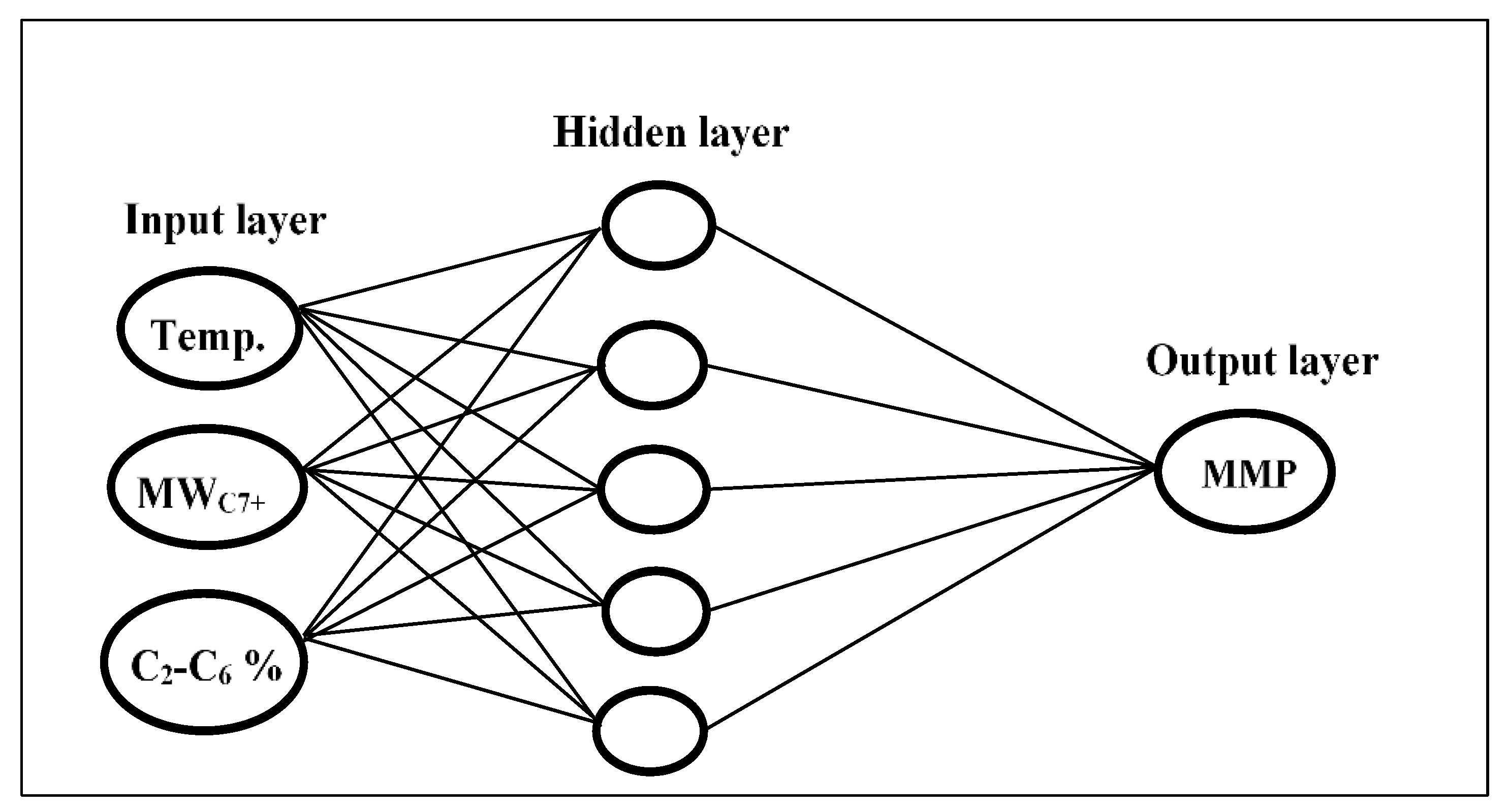
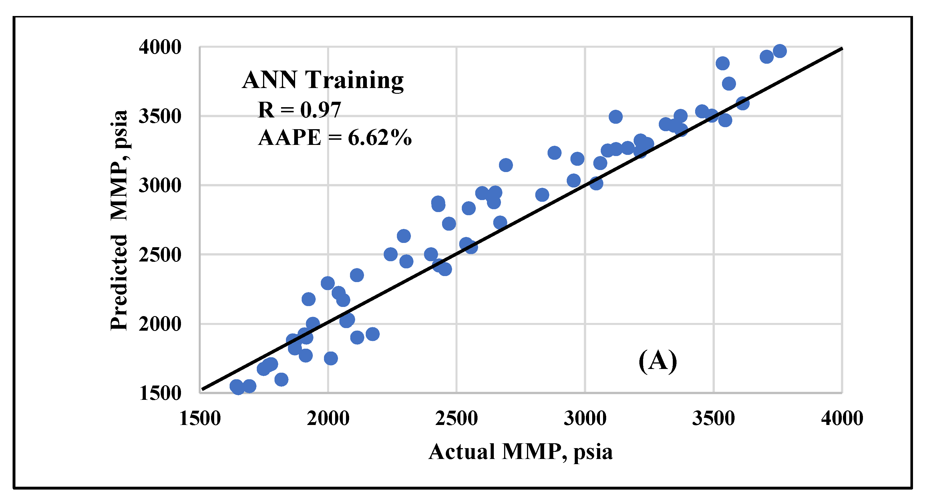
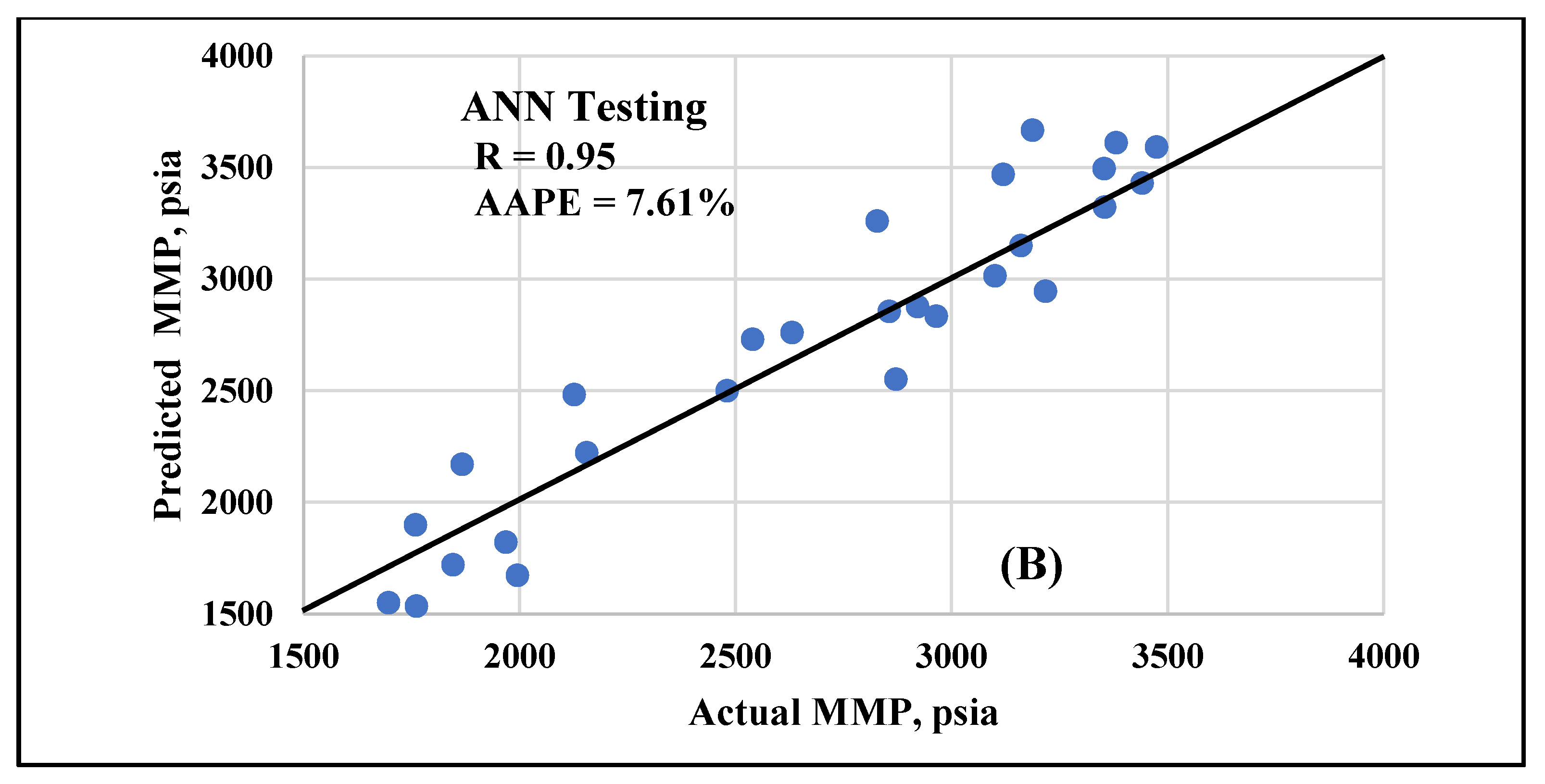
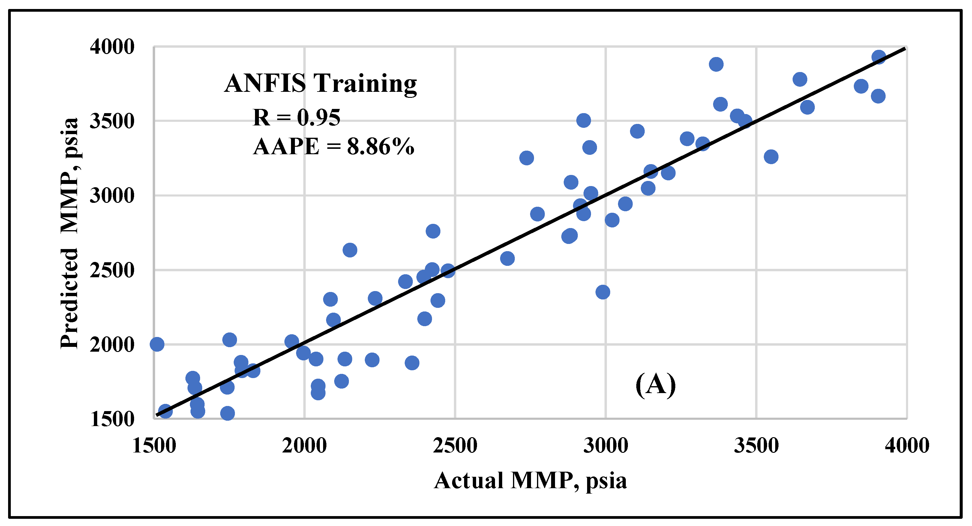
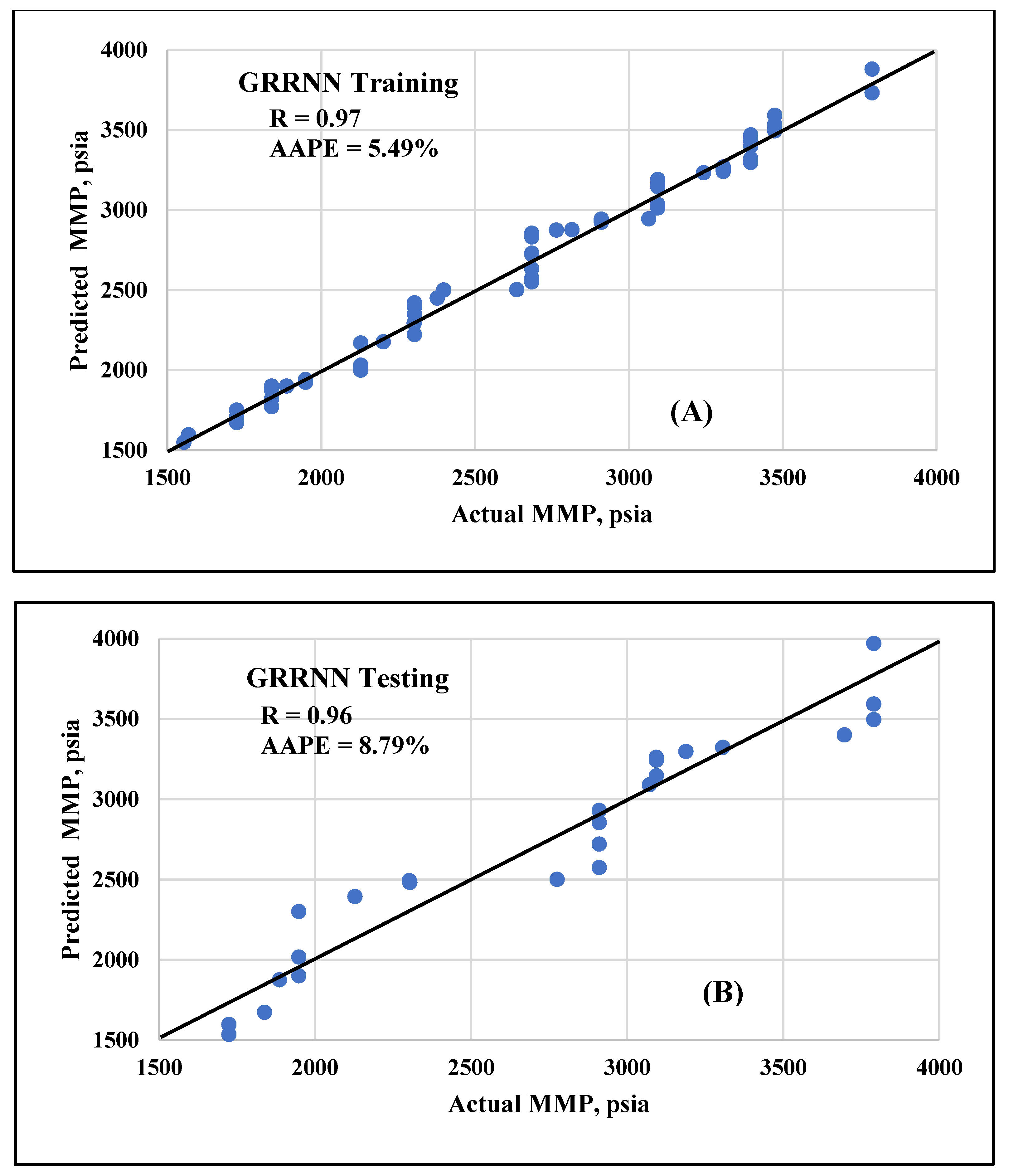
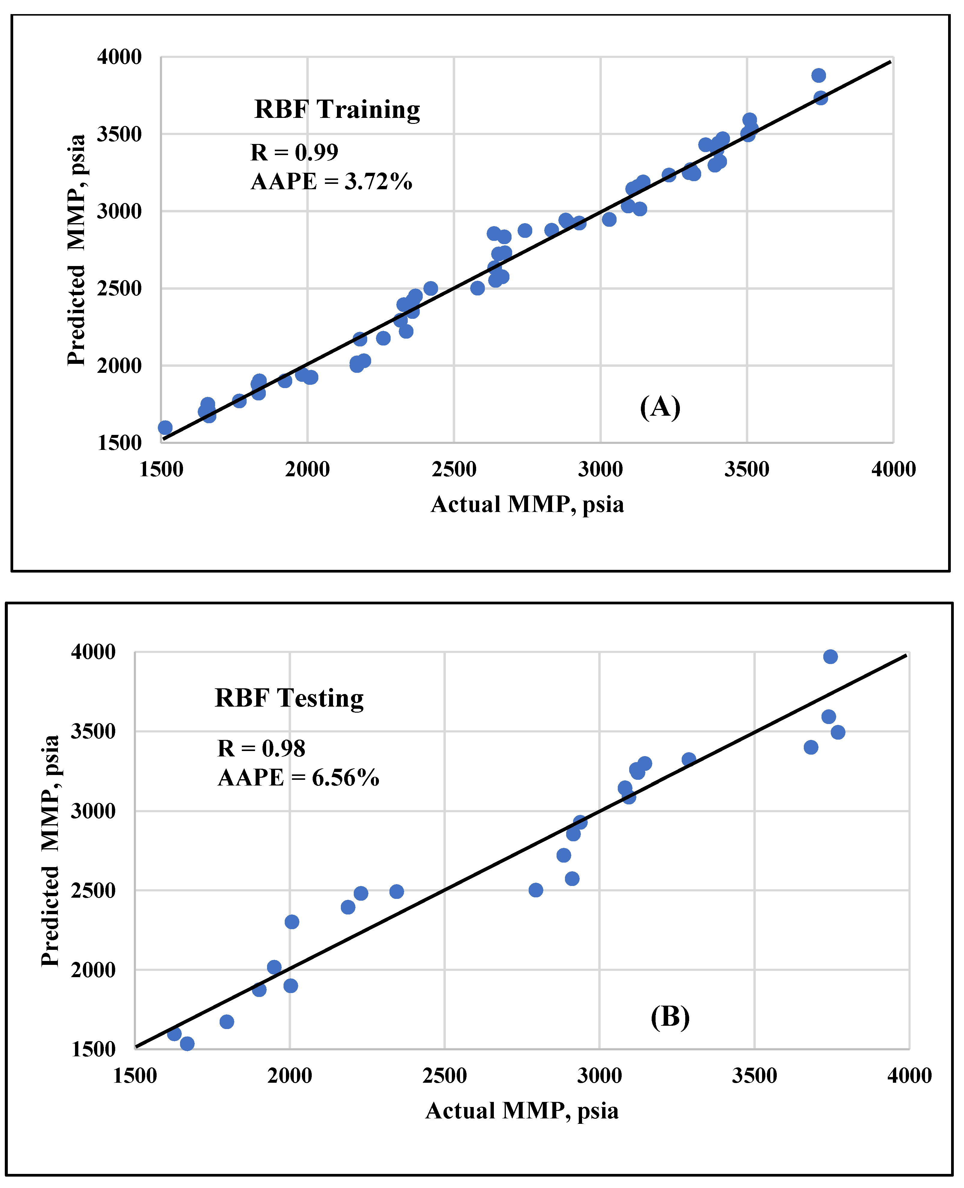
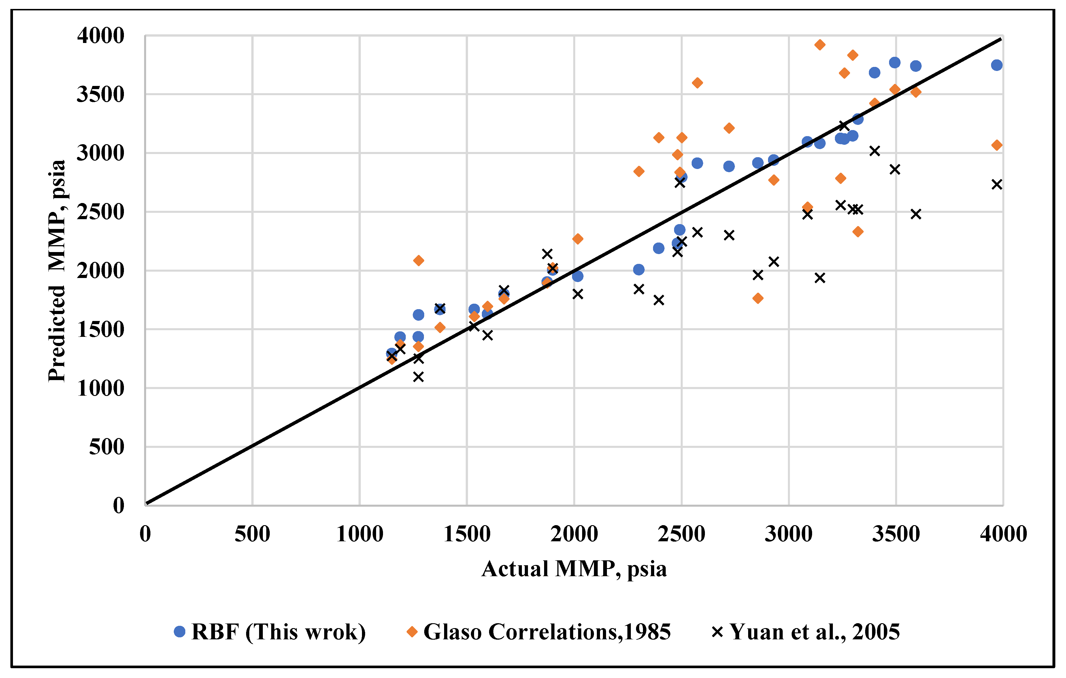
In this paper, a reliable approach is presented to determine the MMP during the CO₂ miscible flooding. Several artificial intelligence (AI) methods were studied, such as neural network, radial basis function, generalized neural network and fuzzy logic. The studied models investigate the significance of reservoir temperature, oil gravity, hydrocarbon composition and the injected-gas composition on the CO₂-MMP. More than 100 data sets belonging to actual CO₂-MMP experiments were used to develop and investigate the model reliability. This work introduces an effective approach for estimating the MMP during CO₂-flooding, which could be used to refine the current numerical or analytical models and result in a better determination of the CO₂-MMP.

2. Methodology

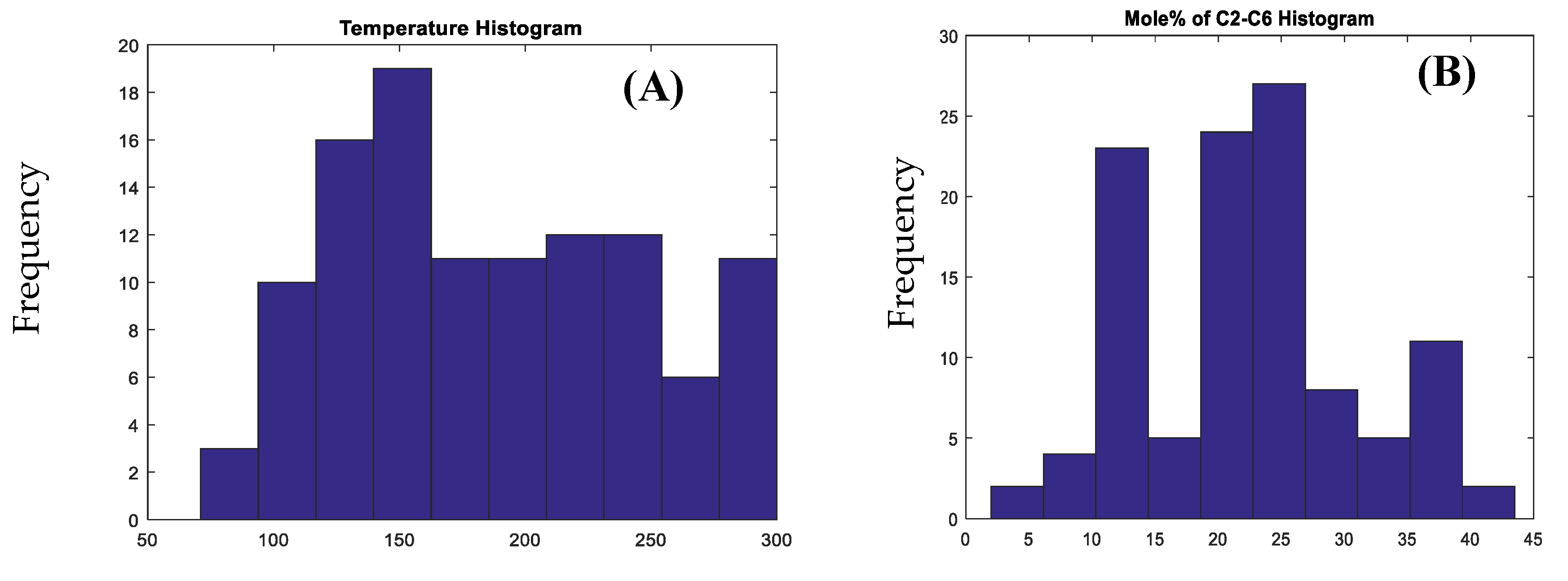
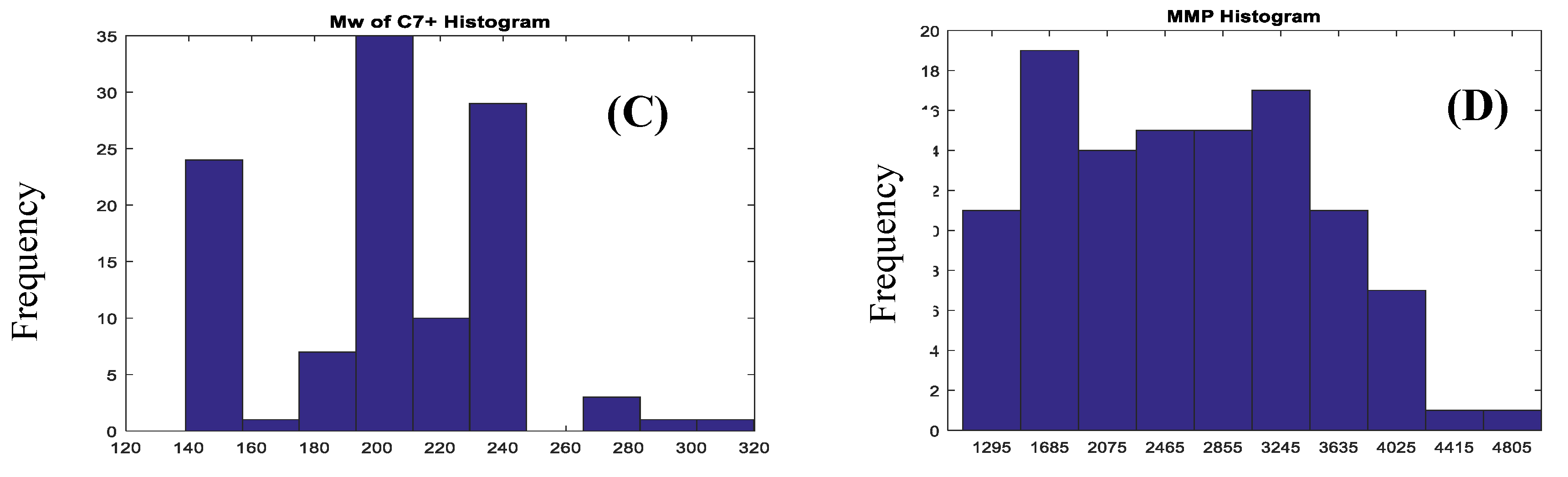
The data used were gathered from several published papers [7,10,14,15,36,37]. The minimum miscibility pressures (MMP) were measured using slim tube tests. The used dataset covers a wider range of reservoir conditions and hydrocarbon compositions; the main inputs are fluid composition, reservoir temperature and molecular weights. The dataset was randomly categorized into two divisions, training group (70% of the total data set) and testing group (30% of the total data). Before developing the AI models, statistical analysis was conducted by determining the minimum, maximum, mean, mode and other parameters, as listed in

Table 1. A statistical analysis of the input and output data used in this study.

Parameter	Temperature, °F	Mole % of C2–C6	MW of C7+	MMP, psia
Minimum	71.00	2.00	139.00	1100.00
Maximum	300.00	43.50	319.70	5000.00
Arithmetic Mean	185.67	22.06	204.85	2583.49
Range	229.00	41.50	180.70	3900.00
Variation	3630.62	73.64	1550.35	769,100.02
Standard deviation	60.25	8.58	39.37	876.98
Skewness	0.23	0.16	−0.11	0.21
Kurtosis	2.00	2.54	2.53	2.20
Coefficient of variation	32.45	38.90	19.22	33.95

. The temperature data is changing in a range of 229 °F with a minimum value of 71 °F, maximum of 330 °F and arithmetic mean of 185.67 °F. The MMP values are changing between 1100 psia to 5000 psia with an arithmetic mean of 2583.49 psia. The statistical dispersion for MMP results was measured by calculating the standard deviation, skewness and kurtosis, and values of 876.98, 0.21 and 2.20 were obtained, respectively, which indicates that the data points are spread out over a wider range of values.

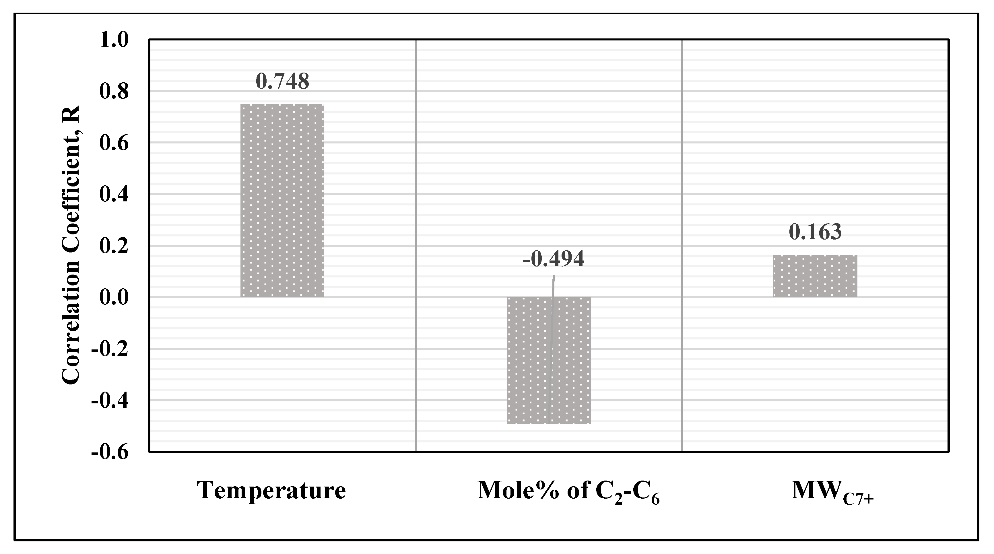
In addition, the frequency histograms were obtained for all data to give a rough estimation for the distribution density. The data set showed a multimodal pattern as shown in Figure 1. Finally, the correlation coefficient was determined to measure the strength and direction of the linear relationship between the input data and MMP data, Figure 2. Values of 0.7481, −0.493 and 0.1626 were obtained for temperature, mole fractions, and molecular weight, respectively, which indicates a weak linear relationship for both the mole fractions and molecular weight. Histogram plots indicate that most of the data set can be represented by the multimodal pattern. The correlation coefficient analysis reveals that the MMP has a weak relationship with the molecular weight, moderate relationship with the mole fractions, and a strong relationship with the system temperature.

The correlation coefficient analysis showed that the molecular weight of C₇₊ and the mole fractions of C₂–C₆ have a small effect on the MMP; however, those parameters are playing a significant role in controlling the MMP. Therefore, to improve these relationships the input data was transformed to different domains using different approaches (i.e., log, power, sigmoidal, etc.) until the best relationships, that have the highest correlation coefficient values, were obtained. Using the power model with power values of −1 and −0.5 for the molecular weight and the mole fraction, respectively, showed the best relationships between the input and output parameters (results are listed in

Table 2. Correlation coefficient analysis for original and power transformed data.

Input Parameters	Correlation Coefficient
	Original Data	Power Transformed
Temperature	0.7481	0.7481
C2–C6%	−0.4935	0.6682
MWC7+	0.1626	0.4982

).

3. Results and Discussion

Different artificial intelligence methods were used to obtain the optimum model that has the lowest average absolute percentage error (AAPE) for both the training and testing data and has the maximum correlation coefficient (R) value. Appendix A illustrates the equations used to calculate the AAPE and R. Sensitivity analysis was performed to fine tune the model parameters; the most suitable models are reported in this paper.

Initially, the original data were used to predict the MMP; however, significant errors were observed for all AI models. For example, the ANN model gave an error of 41.39%, and fuzzy logic system showed an error of 26.14%. Therefore, data processing techniques were implemented, by filtering the data to remove the outlier based on the average values and standard deviation (SD). The input data were also transformed into another domain using a power model. Trial and error technique was used to determine the best combination for the input parameters. Mainly, the fluid composition was categized into two groups: the first group is the mole percentage of ethane to hexane (C₂ to C₆%) and the second group is the molecular weight of heptane plus (MW C₇₊). Then, the square root of the first group (C₂ to C₆%) and the reciprocal of the second group (MW C₇) were used as input parameters. As results of that, the error was reduced significantly, for example, in the ANN model the error decreased from 41.392% to 9.682%. The results from the artificial intelligence techniques are discussed below. Moreover, the problem of local minima was avoided by running the AI models several times using different model parameters. The profile of the error for the training and the testing data sets were also monitored during the phase of model development and validation. The error profiles were used to avoid the model memorization and the local minima problems.

3.1. Artificial Neural Network

Figure 3 illustrates a schematic of the ANN model developed for estimating the CO₂-MMP. The model inputs are reservoir temperature (Temp.), the molecular weight of the heptane plus (MWC₇₊) and the mole fraction of ethane to hexane (C₂–C₆%). The ANN model was trained using the seen data (training dataset), then the model becomes ready to determine the MMP for the testing data (unseen data). The model parameters were fine-tuned to minimize the AAPE and maximize the correlation coefficient. The ANN parameters were fine-tuned by changing the number of hidden layers and the number of neurons per each layer, and the best predictive models listed in

Table 3. Artificial neural network (ANN) for testing results.

No. of Hidden Layers	No. of Neurons in Each Layer	R	AAPE, %
1	20	0.95	7.61
2	20	0.94	10.42
3	20	0.93	12.45

. Three cases were reported, the number of hidden layers and neuron per each layer were varied to find the best ANN model. A minimum error of 7.22% and a relatively high correlation coefficient of 0.974 were obtained by using one hidden layer with 20 neurons. Figure 4 shows the predicted results against the actual values for training and testing data for visual validation.

3.2. Fuzzy Logic System

Different cases were investigated to optimize the model parameters and achieve the best possible model, and the results are represented in

Table 4. Results of using the fuzzy logic system for testing results.

Case No.	Cluster Radius	Number of Iterations	R	AAPE, %
1	0.1	200	0.76	17.09
2	0.3	200	0.86	14.65
3	0.6	200	0.89	10.77
4	0.7	200	0.87	11.61
5	1	200	0.83	13.80
6	0.6	100	0.89	10.58
7	0.6	50	0.89	9.86
8	0.6	10	0.84	13.47

and Figure 5. Correlation coefficients (R) and absolute error (AAPE) for testing data were used to select the optimum model. Increasing the cluster radius led to better results, i.e., increase the R-values and decrease AAPE for the testing data. Increasing the number of iterations led to worse results that could be due to memorization, i.e., decreasing the R-values for testing data; 50 was selected as the optimum value for the iteration number. Case 7 has the lowest AAPE of 9.54%, and can be considered as the best possible model.

3.3. Generalized Neural Network

A generalized neural network (GRNN) was used to determine the CO₂-MMP based on the reservoir temperature and the hydrocarbon composition. This network showed a good performance for predicting the minimum miscibility pressure.

Table 5. Generalized regression neural network (GRNN) results for the testing data.

Case No.	Training Function	Spread	R	AAPE, %
1	newgrnn	1	0.96	9.69
2	newgrnn	10	0.97	8.79
3	newgrnn	50	0.98	16.14
4	newrbe	1	0.97	18.07
5	newrbe	10	0.48	19.76

and Figure 6 summarize the results obtained using the GRNN method. Several cases were investigated to optimize the model parameters. It was found that increasing the spread from 1 to 50 led to improving the R-value from 0.96 to 0.98. Different training functions were also tested, with “newgrnn” showing the highest performance among the others. The best GRNN model (Case 2) showed an error of 7.02% and R-value of 0.98.

3.4. Radial Basis Function

Different model parameters (goal, spread, the maximum number of neurons and number of neurons) were studied to achieve the optimum values. Generally, increasing the goal values mean increasing the model tolerance, leading to increases in the AAPE and a decreased R-value; the same trend was observed for the spread.

Table 6. Radial basis function network (RBF) results for unseen data.

Case No.	Goal	Spread	MN	DF	R	AAPE, %
1	0	100	10	1	0.96	8.98
2	0.5	100	10	1	0.96	8.98
3	1	100	10	1	0.96	8.98
4	0.5	10	20	1	0.98	6.56
5	0.5	100	20	1	0.95	9.84

summarizes the obtained results for 5 cases. For this data set, the goal showed a minor effect in obtaining a better solution, and the value of 0.5 is selected for the goal. Reducing the spread has a positive effect in improving the solution, spread of 10 is selected. Increasing the MN (maximum number of neurons) led to memorization and then reduced the R-value, and 20 MN is selected as an optimum value. The number of neurons to add between displays (DF) has a small effect in improving the model accuracy; a DF of 1 is selected. Based on the previous analysis, the optimum case could be obtained by using the goal of 0.5, the spread of 10, MN of 10 and DF of 1, the obtained R is 0.98 and the AAPE is 6.56% (Case 4); the obtained results are shown in Figure 7.

3.5. Validation of the Developed Model

The radial basis network was utilized to extract an empirical correlation, the weights of the hidden layer (w₁) and the output layer (w₂) were used to derive the empirical equation, and the values are listed in

Table 7. The developed RBF-based weights and biases for CO₂-MMP determinations for Equation (2).

No. of Neurons	Input Layer				Output Layer
	Weights (W1)			Biases (b1)	Weights (W2)	Bias (b2)
	x1	x2	x3
i = 1	300	2.0145	4.6110	0.0023	1.191E+11	−3,966,379.393
i = 2	71	0.3679	2.1756	0.0023	−6.700E+08
i = 3	88	0.3667	1.9069	0.0023	−3.196E+10
i = 4	280	1.4368	3.7815	0.0023	7.492E+10
i = 5	110	0.3873	1.5902	0.0023	−9.397E+09
i = 6	250	0.8993	4.5083	0.0023	9.049E+11
i = 7	260	1.3342	3.6439	0.0023	−5.683E+11
i = 8	250	1.0348	4.9060	0.0023	−8.044E+11
i = 9	90	0.4369	1.8974	0.0023	4.042E+10
i = 10	300	1.5394	3.9142	0.0023	−4.105E+11
i = 11	260	1.7459	4.2926	0.0023	4.109E+11
i = 12	300	1.2435	3.4496	0.0023	2.750E+11

. The proposed model to predict the CO₂-MMP is given by the following equations:

$$MMP = \left[{\displaystyle \sum }_{i = 1}^N{w}_{2i}tansig\left({\displaystyle \sum }_{j = 1}^J{w}_{1i,j}{x}_j+b_{1i}\right)\right]+ b_2 ,$$

(1)

$$MMP = \left[{\displaystyle \sum }_{i = 1}^N{w}_{2i}\left(\frac{2}{1+ e^{-2\left(w_{1i,1}{\left(x1\right)}_j+ w_{1i,2}{\left(x2\right)}_j+ w_{1i,3}{\left(x3\right)}_j+b_{1i}\right)}}\right)\right]+ b_2 .$$

(2)

Equation (2) is an empirical equation extracted from the optimized radial basis model; this equation can be used to estimate the MMP during CO₂ flooding. Similar equations were developed before based on the weights and biases for determining several parameters as reported by Elkatatny et al., Moussa et al., Mahmoud et al. and Rammay and Abdulraheem [23,24,25,38]. In Equations (1) and (2), N is the total neurons number, j is the input index, x1, x2, x3 are the reservoir temperature, the mole fraction of C₂ to C₆, and the molecular weight of heptane plus a fraction, respectively. The weights (w) and biases (b) are listed in Table 7. The developed model normalizes the input data automatically into a range between −1 and 1 based on the two-points method. Equations (3) and (4) are used to calculate the normalized values:

$$\frac{Y- Y_{min}}{Y_{max}- Y_{min}} = \frac{X- X_{min}}{X_{max}- X_{min}},$$

(3)

$$Y =Y_{min}+ \left(Y_{max}- Y_{min}\right)\left(\frac{X- X_{min}}{X_{max}- X_{min}}\right).$$

(4)

Furthermore, a comparison study was performed between the different MMP determination approaches. CO₂-MMP was determined using the Glaso [8] empirical correlation, the Yuan et al. [15] analytical method and the developed AI model. Figure 8 and

Table 8. Determination of CO₂-MMP using different approaches.

Determination Approach	R	AAPE, %
Correlation	0.67	16.4
Analytical	0.60	16.7
RBF model (this work)	0.98	6.6

summarize the obtained CO₂-MMP. The absolute error and correlation coefficient were used to select the best determination approach. Yuan et al.’s [15] analytical equation showed the highest error (16.7%) and the lowest correlation coefficient (0.60) among all approaches. Absolute error of 16.4% and correlation coefficient of 0.67 were obtained using the Glaso [8] empirical correlation, which indicates that those equations (Yuan et al. and Glaso 1985) were developed based on limited experimental results and several assumptions were applied. The AI model of radial basis function showed the best prediction performance, the absolute error and the correlation coefficients are 6.6% and 0.98 respectively. Based on this study, the recommended approach for predicting the CO₂-MMP is an AI model with a radial basis function.

In addition, real case studies for the flooding of hydrocarbon reservoirs with carbon dioxide were used. The data were collected from Kanatbayev et al. and Alomair et al. [39,40]. The CO₂ minimum miscibility pressure was determined using the developed AI model, numerical simulation and regression techniques. Numerical approach (in Eclipse 300) was utilized to determine the CO₂-MMP, the reservoir system was segmented into 2000 grid blocks, and the numerical dispersion was corrected using the infinite cell solution [39]. Alternating conditional expectation (ACE) regression algorithm was used to predict the CO₂-MMP, the regression algorithm was proposed by Alomair et al., 2015 [40]. The predicted MMP values were compared with the actual values that were measured using slim tube tests. The actual minimum miscibility pressures and the predicted values were calculated by different methods and, in addition to the error values, are listed in

Table 9. Actual and predicted values of the minimum miscibility pressures.

Case Number	Actual MMP, Psi	Regression Approach		Numerical Approach		The Developed AI Model
		MMP, Psi	Error, %	MMP, psi	Error, %	MMP, psi	Error, %
1	3974.0	3319.3	16.5	3556.9	10.5	4264.7	7.3
2	2407.6	2203.3	8.5	2010.8	16.5	2605.9	8.2
3	4728.2	3810.6	19.4	3909.4	17.3	5138.6	8.7
4	4351.1	3531.1	18.8	3752.1	13.8	4674.5	7.4
5	4380.1	4122.3	5.9	4993.4	14.0	4720.8	7.8
6	2860.1	2637.4	7.8	3342.5	16.9	3064.2	7.1
7	4677.5	4519.6	3.4	5485.6	17.3	5077.0	8.5
8	4890.7	4730.3	3.3	4083.3	16.5	5311.8	8.6
9	4496.2	3619.5	19.5	5126.8	14.0	4892.1	8.8
10	4278.6	3682.6	13.9	4995.9	16.8	4553.8	6.4
11	4496.2	3763.0	16.3	5193.4	15.5	4903.0	9.0
12	4322.1	3926.4	9.2	4989.6	15.4	4662.8	7.9
13	4119.1	3788.7	8.0	3737.0	9.3	4457.5	8.2
14	4612.2	3771.1	18.2	5141.2	11.5	4953.3	7.4
15	4554.2	4511.1	0.9	5117.8	12.4	4865.6	6.8
16	4844.3	3973.1	18.0	4190.9	13.5	5221.1	7.8
17	4960.3	4866.0	1.9	4465.9	10.0	5338.9	7.6
18	4568.7	4468.9	2.2	5003.9	9.5	4891.7	7.1
19	2523.7	2477.1	1.8	2875.9	14.0	2734.2	8.3
20	3190.8	2847.2	10.8	2912.6	8.7	3397.2	6.5

. Average absolute error of 10.2% was obtained using the regression approach, and errors between 8.7% to 17.3% were obtained using the numerical approach (Eclipse 300). The developed AI model in this study showed an acceptable prediction performance, with the absolute error varying between 6.4% to 9%.

4. Conclusions

This paper presents an intelligent model for determining the minimum miscibility pressure (MMP) during CO₂ flooding. Artificial intelligence (AI) techniques were used to build a new MMP model. A neural network, radial basis function, generalized network and fuzzy logic system were used. The best predictive model was selected based on the absolute error and the correlation coefficient for the testing data set. Based on this work, the following points can be drawn:

• The proposed AI models are quick, rigorous and outperforms the current CO₂-MMP methods. The developed models can minimize the time and cost of determining the CO₂-MMP.
• The developed models investigate the effect of hydrocarbon component and the injected gas composition on the MMP during CO₂-flooding.
• A new equation was extracted using the optimized radial basis function, the developed equation showed a good performance for determining the CO₂-MMP, and the absolute error is 6.6% and the correlation coefficient is 0.98.
• Ultimately, this work will improve the design of CO₂ flooding operations by providing a reliable value for the CO₂-MMP.

References

1. Cronquist, C. Carbon dioxide dynamic displacement with light reservoir oils. In Proceedings of the Fourth Annual US DOE Symposium, Tulsa, OK, USA, 28 August 1978; pp. 18–23. [Google Scholar]
2. Yellig, W.F.; Metcalfe, R.S. Determination and Prediction of CO2 Minimum Miscibility Pressures (includes associated paper 8876). J. Pet. Technol. 1980, 32, 160–168. [Google Scholar] [CrossRef]
3. Shi, Q.; Jing, L.; Qiao, W. Solubility of n-alkanes in supercritical CO2 at diverse temperature and pressure. J. CO2 Util. 2015, 9, 29–38. [Google Scholar] [CrossRef]
4. Holm, L.W.; Josendal, V.A. Effect of oil composition on miscible-type displacement by carbon dioxide. Soc. Pet. Eng. J. 1982, 22, 87–98. [Google Scholar] [CrossRef]
5. Czarnota, R.; Janiga, D.; Stopa, J.; Wojnarowski, P. Determination of minimum miscibility pressure for CO2 and oil system using acoustically monitored separator. J. CO2 Util. 2017, 17, 32–36. [Google Scholar] [CrossRef]
6. Sebastian, H.M.; Wenger, R.S.; Renner, T.A. Correlation of minimum miscibility pressure for impure CO2 streams. J. Pet. Technol. 1985, 37, 2–076. [Google Scholar] [CrossRef]
7. Alston, R.B.; Kokolis, G.P.; James, C.F. CO2 minimum miscibility pressure: A correlation for impure CO2 streams and live oil systems. Soc. Pet. Eng. J. 1985, 25, 268–274. [Google Scholar] [CrossRef]
8. Glaso, O. Generalized minimum miscibility pressure correlation. SPE J. 1985, 25, 927–934. [Google Scholar]
9. Khazam, M.; Arebi, T.; Mahmoudi, T.; Froja, M. A new simple CO2 minimum miscibility pressure correlation. Oil Gas Res. 2016, 2. [Google Scholar] [CrossRef] [Green Version]
10. Yuan, H.; Johns, R.T.; Egwuenu, A.M.; Dindoruk, B. Improved MMP correlation for CO2 floods using analytical theory. SPE Reserv. Eval. Eng. 2005, 8, 418–425. [Google Scholar] [CrossRef]
11. Johns, R.T.; Dindoruk, B.; Orr, F.M., Jr. Analytical theory of combined condensing/vaporizing gas drives. SPE Adv. Technol. Ser. 1993, 1, 7–16. [Google Scholar] [CrossRef]
12. Dindoruk, B.; Orr, F.M., Jr.; Johns, R.T. Theory of multi-contact miscible displacement with nitrogen. SPE J. 1997, 2, 268–279. [Google Scholar] [CrossRef]
13. Jessen, K.; Michelsen, M.L.; Stenby, E.H. Global approach for calculation of minimum miscibility pressure. Fluid Phase Equilibria 1998, 153, 251–263. [Google Scholar] [CrossRef]
14. Yuan, H. Application of Miscibility Calculation to Gas Floods. Ph.D. Thesis, The University of Texas at Austin, Austin, TX, USA, 2003. [Google Scholar]
15. Yuan, H.; Johns, R.T.; Egwuenu, A.M.; Dindoruk, B. Improved MMP correlations for CO2 floods using analytical gas flooding theory. Presented at the 2004 SPE Symposium on Improved Oil Recovery, Tulsa, OK, USA, 17–21 April 2004. SPE 89359. [Google Scholar]
16. Venkatraman, V.; Alsberg, B.K. Predicting CO2 capture of ionic liquids using machine learning. J. CO2 Util. 2017, 21, 162–168. [Google Scholar] [CrossRef]
17. Sargolzaei, J.; Saghatoleslami, N.; Mosavi, S.M.; Khoshnoodi, M. Comparative Study of Artificial Neural Networks (ANN) and statistical methods for predicting the performance of Ultrafiltration Process in the Milk Industry. Iran. J. Chem. Eng. 2006, 25, 67–76. [Google Scholar]
18. Sedghamiz, M.A.; Rasoolzadeh, A.; Rahimpour, M.R. The ability of artificial neural network in prediction of the acid gases solubility in different ionic liquids. J. CO2 Util. 2015, 9, 39–47. [Google Scholar] [CrossRef]
19. Al-Shehri, D.A. Oil and Gas Wells: Enhanced Wellbore Casing Integrity Management through Corrosion Rate Prediction Using an Augmented Intelligent Approach. Sustainability 2019, 11, 818. [Google Scholar] [CrossRef] [Green Version]
20. Mahmoud, A.A.; Elkatatny, S.; Ali, A.; Moussa, T. Estimation of Static Young’s Modulus for Sandstone Formation Using Artificial Neural Networks. Energies 2019, 12, 2125. [Google Scholar] [CrossRef] [Green Version]
21. Elkatatny, S. Real-time prediction of rheological parameters of KCL water-based drilling fluid using artificial neural networks. Arab. J. Sci. Eng. 2017, 42, 1655–1665. [Google Scholar] [CrossRef]
22. Elkatatny, S.; Mahmoud, M.; Tariq, Z.; Abdulraheem, A. New insights into the prediction of heterogeneous carbonate reservoir permeability from well logs using artificial intelligence network. Neural Comput. Appl. 2018, 30, 2673–2683. [Google Scholar] [CrossRef]
23. Elkatatny, S.; Tariq, Z.; Mahmoud, M. Real time prediction of drilling fluid rheological properties using Artificial Neural Networks visible mathematical model (white box). J. Pet. Sci. Eng. 2016, 146, 1202–1210. [Google Scholar] [CrossRef]
24. Moussa, T.; Elkatatny, S.; Mahmoud, M.; Abdulraheem, A. Development of new permeability formulation from well log data using artificial intelligence approaches. J. Energy Resour. Technol. 2018, 140, 072903. [Google Scholar] [CrossRef]
25. Mahmoud, A.A.; Elkatatny, S.; Mahmoud, M.; Abouelresh, M.; Abdulraheem, A.; Ali, A. Determination of the total organic carbon (TOC) based on conventional well logs using artificial neural network. Int. J. Coal Geol. 2017, 179, 72–80. [Google Scholar] [CrossRef]
26. Ali, H.; Choi, J.H. A Review of Underground Pipeline Leakage and Sinkhole Monitoring Methods Based on Wireless Sensor Networking. Sustainability 2019, 11, 4007. [Google Scholar] [CrossRef] [Green Version]
27. Amirian, E.; Leung, J.Y.; Zanon, S.; Dzurman, P. Integrated cluster analysis and artificial neural network modeling for steam-assisted gravity drainage performance prediction in heterogeneous reservoirs. Expert Syst. Appl. 2015, 42, 723–740. [Google Scholar] [CrossRef]
28. Amirian, E.; Fedutenko, E.; Yang, C.; Chen, Z.; Nghiem, L. Artificial Neural Network Modeling and Forecasting of Oil Reservoir Performance. In Applications of Data Management and Analysis; Springer: Cham, Switzerland, 2018; pp. 43–67. [Google Scholar]
29. Malo, S.; McNamara, J.; Volkmer, N.; Amirian, E. Eagle Ford—Introducing the Big Bad Wolf. Presented at the Unconventional Resources Technology Conference, Denver, CO, USA, 22–24 July 2019; pp. 4733–4743. [Google Scholar]
30. Edalat, M.; Dinarvand, N.; Shariatpanahi, S.F. Development of a new artificial neural network model for predicting minimum miscibility pressure in hydrocarbon gas injection. Presented at the 15th SPE Middle East Oil & Gas Show and Conference, Bahrain International Exhibition Centre, Manama, Bahrain, 11–14 March 2007. SPE 105407. [Google Scholar]
31. Dehghani, S.M.; Sefti, M.V.; Ameri, A.; Kaveh, N.S. Minimum miscibility pressure prediction based on a hybrid neural genetic algorithm. Chem. Eng. Res. Des. 2008, 86, 173–185. [Google Scholar] [CrossRef]
32. Shokrollahi, A.; Arabloo, M.; Gharagheizi, F.; Mohammadi, A.H. Intelligent model for prediction of CO2–reservoir oil minimum miscibility pressure. Fuel 2013, 112, 375–384. [Google Scholar] [CrossRef]
33. Liu, Y.; Jiang, L.; Song, Y.; Zhao, Y.; Zhang, Y.; Wang, D. Estimation of minimum miscibility pressure (MMP) of CO2 and liquid n-alkane systems using an improved MRI technique. Magn. Reson. Imaging 2016, 34, 97–104. [Google Scholar] [CrossRef]
34. Rostami, A.; Arabloo, M.; Lee, M.; Bahadori, A. Applying SVM framework for modeling of CO2 solubility in oil during CO2 flooding. Fuel 2018, 214, 73–87. [Google Scholar] [CrossRef]
35. Alfarge, D.; Wei, M.; Bai, B. Data analysis for CO2-EOR in shale-oil reservoirs based on a laboratory database. J. Pet. Sci. Eng. 2018, 162, 697–711. [Google Scholar] [CrossRef]
36. Rathmell, J.J.; Stalkup, F.I.; Hassinger, R.C. A laboratory investigation of miscible displacement by carbon dioxide. Presented at the Fall Meeting of the Society of Petroleum Engineers of AIME, New Orleans, LA, USA, 3–6 October 1971. SPE 3483. [Google Scholar]
37. Shokir, E.M. CO2–oil minimum miscibility pressure model for impure and pure CO2 streams. J. Pet. Sci. Eng. 2007, 58, 173–185. [Google Scholar] [CrossRef]
38. Rammay, M.H.; Abdulraheem, A. PVT correlations for Pakistani crude oils using artificial neural network. J. Pet. Explor. Prod. Technol. 2017, 7, 217–233. [Google Scholar] [CrossRef] [Green Version]
39. Kanatbayev, M.; Meisingset, K.K.; Uleberg, K. Comparison of MMP estimation methods with proposed workflow. Presented at the SPE Bergen One Day Seminar, Bergen, Norway, 22 April 2015. SPE 173827. [Google Scholar]
40. Alomair, O.; Malallah, A.; Elsharkawy, A.; Iqbal, M. Predicting CO2 minimum miscibility pressure (MMP) using alternating conditional expectation (ACE) algorithm. Oil Gas Sci. Technol. Rev. d’IFP Energ. Nouv. 2015, 70, 967–982. [Google Scholar] [CrossRef] [Green Version]
Figure 1. Histograms of input and output data. (A) Reservoir temperature, (B) Mole % of C2–C6, (C) MW of C7+ and (D) CO2-MMP (MMP = minimum miscibility pressure).
Sustainability 11 07020 g001aSustainability 11 07020 g001b
Figure 2. Correlation coefficient analysis: the effect of input parameters on CO2-MMP.
Sustainability 11 07020 g002
Figure 3. Artificial neural network (ANN) model architecture with input, hidden and output layers.
Sustainability 11 07020 g003
Figure 4. Cross plot of actual against predicted CO2-MMP using the ANN model for (A) the training data set and (B) the testing data.
Sustainability 11 07020 g004aSustainability 11 07020 g004b
Figure 5. Cross plot of actual against predicted CO2-MMP using the adaptive neuro-fuzzy inference system (ANFIS) model, for A) Training data set, B) Testing data.
Sustainability 11 07020 g005aSustainability 11 07020 g005b
Figure 6. Cross plot of actual against predicted CO2-MMP using the GRNN model for (A) the training data set and (B) testing data.
Sustainability 11 07020 g006
Figure 7. Cross plot of actual against predicted CO2-MMP using the radial basis function (RBF) model for (A) the training data set and (B) testing data.
Sustainability 11 07020 g007
Figure 8. Comparison between different CO2-MMP determination approaches; numerical, analytical and the developed RBF model.
Sustainability 11 07020 g008