Quantitative Estimation and Spatiotemporal Characteristic Analysis of Price Deviation in China's Housing Market

Abstract

Differences in housing prices and rental prices across cities or regions and the relationship between prices and socioeconomic fundamentals are frequent research foci in urban and real estate economics, but the existing studies on China's housing market rarely consider both housing price and rent. This study provides a framework for a quantitative analysis of a country's housing market from the perspective of supply and demand, and takes China's housing market as a case study. The current study first explores the key factors that affect housing prices and rental prices using data from 202 cities and collected from 2011 to 2014. Then, theoretical values of housing prices and rental prices in each city are estimated, and the spatiotemporal characteristics of deviation of housing prices and rental prices are analysed. The empirical findings of the current study mainly reveal the following three points. First, the determinants of housing prices and rental prices have similarities. Second, the effect of above factors shows obvious spatial heterogeneity. The coefficients of the variables are different between coastal and inland regions, indicating different demand and supply elasticities across regions. Third, the price deviation presents significant spatial agglomeration. Cities with higher price deviations are clustered in the Yangtze River Delta and Beijing-Tianjin-Hebei, while the price deviations are relatively mild in the Pearl River Delta region.

1. Introduction

Real estate plays a relatively important role in the economic activities of countries worldwide. The housing market occupies the highest proportion of the real estate market. Housing assets also occupy significant proportions of family wealth in many developed countries [1,2]. The fluctuations of housing prices and rental prices can significantly influence the macro economy and are directly related to the living quality of families and the overall welfare level of a society.

China is the largest developing economic entity in the world. The development of the housing market in China conforms to general experience and basic law. In other words, a fast economic growth period is accompanied by the growth of housing prices. The housing market in China has certain unique characteristics due to special institutional factors, such as public land ownership and frequent government control over the real estate market. Thus, the differences in housing prices and rental prices across cities or regions provide a valuable opportunity for empirical study to affirm and deepen our understanding of the classic theory. The housing market maintained a high growth rate in terms of scale and price after the market-dominated housing supply system was determined in China in 1998. The degree of transaction activity of the real estate market, especially the housing market, remains high, even though the growth of China’s macroeconomy is under strong downturn pressure. According to the data of the State Statistics Bureau, the average marketing price of commercial residential buildings in 2010 was 4,725.0 RMB/m², which increased by 52.44% to 7,203 RMB/m² in 2016. The sharp growth rate of housing prices intensified the housing burden of residents and increased anxiety among stakeholders regarding the financial risks of real estate. Many popular cities implemented measures to inhibit the growth of housing prices by focusing on “purchase limits” and “credit limits.” The 19th CPC National Congress proposed the implementation of a housing system that ensures supply through multiple sources, provides housing support through multiple channels, and encourages house purchasing and renting. This proposed action will enable China to address the housing needs of its people. As China has a vast territory and many cities, there are great differences in economic and social development across regions and cities. It is of great significance for market supervision and decision-making departments to grasp the characteristics of housing prices and rental prices in different cities or regions and judge the reasonability of the current housing prices and rental prices in different cities or regions when implementing targeted management measures. Therefore, a study focusing on identifying the influencing factors of housing prices and rental prices, exploring the differences between the residential real estate market and the rental housing market in China and presenting the spatiotemporal characteristics of the price deviation and its changes is necessary.

According to the supply–demand analysis framework [3,4,5,6], the growth of housing prices and rental prices in cities are highly related to several fundamental factors, such as economic growth, improvement of living quality, and population mobility. Therefore, the rapid growth of housing prices (or a high price) must not be accompanied by increased risks. Researchers should focus on which cities’ housing prices or rental prices deviate seriously from the socioeconomic fundamentals and which cities’ housing prices or rental prices do not. However, the existing studies on housing price deviations in China mainly focuses on 35 large and medium-sized cities rather than on overall analysis, and little attention has been paid to rental prices deviation. The present study establishes an econometric model according to the supply–demand framework based on data from 202 cities collected from 2011 to 2014 to examine the problems mentioned above. The originality and contribution focus on three aspects. First, the size of the urban sample is expanded to reflect the overall situation of the country and regional differences. Second, the GTWR (Geographically and Temporally Weighted Regression) model is used to analyse the spatiotemporal heterogeneity of the factors affecting housing prices and rental prices, and to understand the differences between the Chinese housing market and the rental market. Third, the spatiotemporal characteristics of house prices and rental prices deviations are analysed, and references for the regulation policy of the real estate market are provided.

2. Literature Review

To recognize the decision factors regarding the differences in housing prices and rental prices across cities, the academic circle established an analysis framework that combines supply and demand and achieved rich theoretical and empirical research outcomes [3,4,5,6,7,8]. Ozanne and Thibodeau were the first to establish the supply–demand equilibrium analysis framework of housing price and rental prices in different study cities. They proposed that the long-term equilibrium housing price of a city is the function of supply and demand, and the differences in housing price and rental prices across cities are the consequence of differences in the supply or demand [5]. Rosen and Robcak studied wage differences across cities and proved the existence of a living quality equilibrium for families across cities [9,10]. Roback expanded the analysis to housing markets in cities. He concluded that the differences in housing price across cities can be divided into wage and urban amenity differences [9]. Manning used previous studies as the basis to construct a model that interprets the housing price differences across cities. He set the demand as the function of the real monetary income of a family, the nonmonetary income of family, and a preference between these two factors [3,4]. He enlisted the urban amenity proposed by Roback into the nonmonetary income, which influences demand and sets the supply into the function of the construction costs and available land resources in cities. Potepan constructed a model involving housing price, rent, and land price on the basis of the supply–demand framework. An empirical study using the statistical data of 58 cities in the USA from 1974 to 1983 was conducted. This study found that the median income, population, construction cost, climate, and public service quality were important factors that explain the differences in housing prices and rental prices across cities [6]. Antoniucci and Marella examined the effect of immigrant population on urban house price polarization using data from 112 Italian provincial capitals, and proved that larger immigrant populations will result in nationwide steeper housing price gradients [11]. Egner and Grabietz explored the driving factors of rent prices in German cities using the same framework using time-series analysis, and found that the share of students and the local mean income account for differences in quoted rent prices [12]. In recent years, some scholars have also expanded this basic analysis framework by including factors related to urban residents’ expectations. For instance, Soo, C. K. developed measures of housing sentiment for 34 cities across the United States and found that housing media sentiment has significant predictive power for future house prices [13]. Howard and Liebersohn constructed an asset-pricing theory to explain why regional income divergence explains much of the variation in U.S. house prices [14].

Housing prices will not constantly be equal to the long-term equilibrium level decided by the supply–demand fundamentals, but they may deviate to varying degrees due to short-term fluctuations [15,16,17,18]. The growth of the asset price develops bubbles when it cannot be explained by changes of fundamentals [19,20]. To calculate the deviation of the housing price and determine whether bubbles exist in the real estate market, the price decided by the fundamentals must be measured [21]. The supply–demand analysis framework is one of the methods used to estimate the theoretical price determined by fundamentals. Many scholars studied how the real estate market operates in different countries using this perspective [17,19,21,22,23]. Stevenson estimated the fundamental housing price in Ireland from 1995 to 2003 according to the demand model; they found that most housing price fluctuations in Ireland in the late 1990s were supported by economic and population fundamentals [21]. However, this study focused on the overall national conditions without considering the differences across study regions. Case and Shiller explained the most serious housing price fluctuations in eight states in the USA from 1985 to 1999 using six fundamental variables, namely, population growth, unemployment rate, per capita income, and newly constructed houses. The results were used to predict housings price from 1999 to 2002; they found that the supply–demand fundamentals significantly underestimate the actual growth of housing prices [19]. Meanwhile, Goodman and Thibodeau estimated the housing supply–demand elasticity in different cities in the USA based on the fundamental supply–demand data from 1990 to 2000. Next, the expected housing price growth rate in 84 cities from 2000 to 2005 was calculated according to supply–demand elasticity. The actual growth rate of 25 cities exceeded the expected growth rate of 30%, and housing price bubbles had evident regional concentrations [17]. A few studies have pointed out that places with a small supply elasticity easily develop speculative activities and housing price bubbles [22,24].

These research frameworks have been widely applied to study the housing market in China and analyse the relationship between housing prices and fundamentals to achieve rich research outcomes [25,26,27,28,29,30,31,32]. For example, Li and Chand studied the influences of the supply–demand fundamental on housing prices based on the panel data of 29 provinces from 1998 to 2009. They discovered that income level, construction cost, holding cost, and land price served as the fundamental factors that influence housing prices. Moreover, they found that provinces with developed economies were sensitive to supply factors [26]. Wu, Gyourko, and Deng selected and constructed several supply and demand indexes, such as the housing inventory–sale ratio, construction cost, residential land supply, housing price level in the previous period, and expected export growth. Based on the regression of panel data in 35 large- and middle-sized cities from 2006 to 2013, they found that the inventory-sale ratio, housing price level in the previous period, and expected export growth could significantly influence the growth rate of housing prices [29]. Dreger and Zhang investigated the relationship between housing price fluctuations and macroscopic economic fundamental factors in 35 large and middle-sized cities. They reported the existence of a co-integration relationship between the actual housing prices and actual per capital income, and the actual land price and actual interest rate. The analysis of residual error showed that the deviations in housing prices from the equilibrium values were controlled within 15% in most cities from 2008 to 2010, but were relatively high in some southeast coastal cities and special economic zones [25]. Wang and Zhang set the equilibrium growth rate of housing prices in cities as the function of supply factors (growth of the residential land supply amount and construction costs in cities) and demand factors (per capital income growth and population growth) using the supply–demand analysis framework. The gap between the equilibrium growth rate and actual growth rate in 35 cities was discussed. The research demonstrated that housing price fluctuations in most cities can be explained by changes in the supply–demand fundamentals [28]. However, the housing price growth rates in a few coastal cities deviated significantly from the predicted growth rates. In summary, estimating the long-term equilibrium value and then comparing it with the actual value is the main principle to judge the deviation of housing prices [17,19,21,25,28]. Estimated prices are usually predicted by a reduced form of the formal model under the supply-demand framework. The choice of variables in the reduced form model is based on existing studies, the context of specific countries, and data availability. The coefficients of the variables are estimated by different methods, such as directly regressing housing prices on fundamental factors using OLS [19,21] or the Error Correction Model [25], inferring each coefficient separately from income and the housing demand price elasticities and other parameters [28]. In terms of model selection, most existing studies use the global panel model and the fixed effect model to estimate the factors influencing housing prices. The problem of using the global model is that the effects of the variable remain constant over time and space. However, in the study of the inter-city real estate market, regional differences are obvious. The assumptions of spatial and temporal stationarity are not realistic, and the parameters tend to vary over the study area, especially within large markets. [33,34,35]. The geographically weighted regression (GWR) is a common method for capturing spatial heterogeneity [36], and it outperforms the spatial expansion method in terms of explanatory power and predictive accuracy [37]. It has been applied to the research of China's real estate market [38], but the GWR model are commonly used for cross-sectional data. Although some studies developed expanded version of the cross-sectional GWR analysis to panel data, the method assumes bandwidths and weights generated from the kernel function will remain temporally invariant [39,40,41]. The geographically and temporally weighted regression (GTWR) model incorporates time factors based on the GWR model [33] and can be used to estimate panel data.

Two major conclusions could be drawn from the literature review. First, there is a most common theoretical foundation and analytical framework for the long-term equilibrium values of housing prices and rents in different cities. And the most basic factors should be considered in to empirical studies are from the supply side (e.g., land price, construction cost, land supply, and supply limit), as well as demand side (e.g., population, income, and amenities). Second, in the larger real estate market, the traditional global regression model has difficulty reflecting the spatial heterogeneity of the influencing factors. Using the local regression model is not only able to reflect the spatial heterogeneity of the influencing factors but can also improve the accuracy of the estimation. The studies on the relationship between the urban housing market and fundamentals in China can be improved in the following aspects. First, the sample cities in previous studies were mainly limited to 35 large and middle-sized cities. China has an extensive territory. Significant differences exist in terms of the natural environment, economic, and social development level, and government regulations across different regions and cities in China. Although the 35 large and middle-sized cities cover most regions, they are mainly municipalities and provincial capitals. These areas cannot accurately represent the overall situation of Chinese cities. Second, only a few empirical studies have thoroughly explored the rental housing market in China. The rental housing market is an important submarket of the urban real estate market. Given the accelerating urbanization process in China, the role of the rental housing market cannot be ignored in the background of the decline in the affordability of housing in hotspot cities. Third, in the global model, the influence of the variables average over space and time, so the spatial heterogeneity of the influencing factors cannot be captured.

The research innovation of this study focuses on three aspects. First, the differences between the residential real estate market and the rental housing market in China are compared. Second, the GTWR model is used to improve the explanatory power and to quantify and analyse the spatiotemporal heterogeneity of the influencing factors. Third, the spatiotemporal characteristics of price deviations are analysed, which could provide references for policy decisions regarding the housing market.

3. Materials and Methods

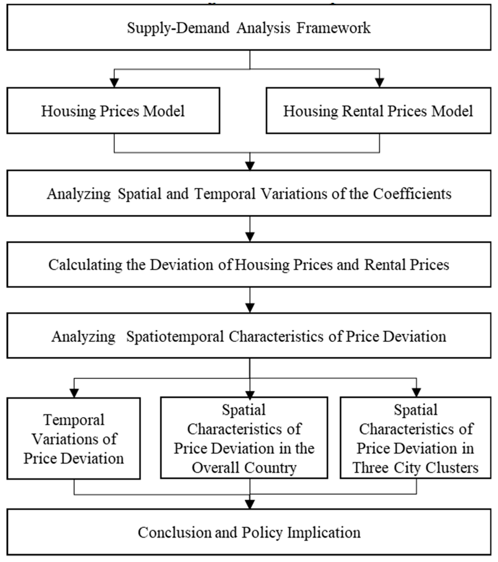
3.1. Research Process

This study will be carried out in accordance with Figure 1. In the first step, based on the supply–demand analysis framework, the existing literature, and the Chinese context, we select the variables to construct the housing price and rental prices model. The second step is to use the data of 202 cities to determine the key factors that affect housing prices and rental prices, estimate the coefficients of all variables, and calculate the estimated values of housing prices and rental prices of each city. Third, the house prices and rental prices deviations according to the estimated values and actual values of the house prices and rental prices in each city are calculated. Fourth, the spatiotemporal characteristics of the house prices and rental prices deviations are presented, and possible reasons for the deviations are discussed. Finally, the results of models and the spatiotemporal characteristics of the price deviations are discussed and compared with the results of existing studies, and some policy recommendations for real estate market management are put forward.

3.2. Method of Price Deviation Estimation

The housing price or rental price (P_i,t) of one city consists of an estimated theoretical value of housing prices or rental prices (P*_i,t) and the deviation from the estimated value (μ_i,t). The literature review indicates that P*_i,t shall be decided by the supply (S_i,t) and demand (D_i,t) of the urban housing market.

$$P_{i,t}=P_{i,t}^{*}+{\mu }_{i,t}$$

(1)

$$P_{i,t}^{*}=f\left(S_{i,t},D_{i,t}\right)$$

(2)

The supply and demand of the housing market are sensitive to exogenous variables. In the present study, the variables are selected based on the supply–demand analysis framework [3,4,5] by combining the existing literature with the actual situation in China. The econometric model is constructed to explore the key influencing factors of housing prices and rental prices and their degrees of influence. P*_i,t is predicted by this econometric model. Next, the deviation value of P_i,t from P*_i,t is calculated as μ_i,t in Equation (1). The deviations of housing prices or rental prices reflect the operating situations of the urban housing market from the perspectives of the house sales and rentals. A high absolute value of the deviation results in a low operating quality of the urban housing market. A positive or negative deviation value shows that the actual housing prices or rental prices in cities are higher or lower than the estimated value. The specific calculation formula is given by the following:

$$\mathrm{Deviation}\mathrm{of}\mathrm{housing}\mathrm{prices}\mathrm{or}\mathrm{rental}\mathrm{prices}=\frac{P_{i,t}-P_{i,t}^{*}}{P_{i,t}^{*}}$$

(3)

3.3. Geographically and Temporally Weighted Regression Model

The GWR model considers the spatial heterogeneity of the parameter estimates by constructing a spatial weight based on the distance determined by (x, y) between an observation point and all other observation points. Temporal effects can also lead to nonstationarity in real estate prices, but the GWR model can only estimate the data of different years separately. Some scholars have further incorporated time information into the GWR model [33], which accounted for the spatiotemporal heterogeneity in the parameter estimates by constructing the weight based on the distances determined by the (x, y, t) coordinates between observation i and all other observations. GTWR captures both the spatial and temporal heterogeneity and improves the explanatory power. The GTWR model can be expressed as follows:

$${\mathrm{Y}}_i={\beta }_0\left(u_i,v_i,t_i\right)+{\displaystyle \sum }_k{\beta }_k\left(u_i,v_i,t_i\right)X_{ik}+{\epsilon }_i$$

(4)

where $\left(u_i,v_i,t_i\right)$ denotes the coordinates of the point i, ${\beta }_0\left(u_i,v_i,t_i\right)$ represents the intercept value, and ${\beta }_k\left(u_i,v_i,t_i\right)X_{ik}$ is a set of values of the parameters at point i. Unlike the global model, this model allows the parameter estimates to vary across space and time and is, therefore, likely to capture local effects. Essentially, the problem here is to provide estimates of ${\beta }_k\left(u_i,v_i,t_i\right)$ for each variable k and each spatiotemporal location i. Spatio-temporal bandwidth should be determined before estimation. The bandwidth in the GTWR model determines the rate at which the regression weights decay around a given point $\left(u_i,v_i,t_i\right)$. It is important to choose a suitable bandwidth to obtain accurate estimates of coefficients. Cities are distributed sparsely in some areas, but densely in other areas. To avoid exaggerating the degree of nonstationarity in the areas where data are sparse or mask subtle spatial nonstationarity where the data are dense, adaptive function are used [42]. The spatial context (the Gaussian kernel) is a function of a specified number of neighbours. Kernels have larger bandwidths where the data points are sparsely distributed, and have smaller bandwidths where the data are dense. The optimal neighbour parameter will be searched using cross-validation (CV) criteria [33]. This study uses the GTWR model plugin in Arcgis 10.2 developed by Huang et al. to process the data.

3.4. Empirical Analysis Framework and Model

The common variables in the demand factors, which influence the long-term equilibrium level of housing prices and rental prices, include income, population size, employment, and amenity [3,4,6,16]. The current study measures income and employment by urban per capita disposable income and the proportion of employed persons in tertiary industries. Despite the local population size, the inflow of foreign populations will increase the demand for houses, thereby increasing housing prices and rent [43,44]. The recent rapid progress in China’s urbanization has caused large rural populations to migrate to the cities. The migration of huge populations from small- to large-sized cities results in huge demands for housing purchases and rental in the destination cities. The current study uses the permanent resident population size and proportion of the net inflow in permanent resident population to measure the population size and population flow, respectively. An amenity is a nonmonetary income gained from a city [9], which is often divided into natural amenities and public service quality. Cities with good climate and public resources, such as education, health care, and culture, can attract additional population. The current study measures the climate by the difference in annual temperature. Public resources are measured by variables constructed from Public Service Quality (PSQ) related to education, health care, and public transportation.

The existing studies on housing prices in China considered the impacts of monetary income [28,29,30,45], but only a few have fully considered nonmonetary income (e.g., amenities). Given that there are many existing variables that can reflect PSQ in cities and that they are highly mutually correlated, serious multicollinearity can occur if they are used in the model. To solve this problem, the comprehensive variables of PSQ in cities are constructed by factor analysis. Factor analysis enables most information of the original data to be reflected by a few principal components. The current study selects 15 indexes from five aspects (education, health care, public transportation, entertainment, and environment,

Table 1. Indexes Used to Construct the Public Service Quality.

Variable	Dimensions	Indexes
Public Service Quality	Education [49,50,51,52,53]	Number of Primary Schools
		Number of Regular Secondary Schools
		Number of Regular Institutions of Higher Education
		Teacher–student Ratio in Primary Schools
		Teacher–student Ratio in Regular Secondary Schools
		Expenditure for Education per capita
	Health Care	Number of Hospitals and Health Centres per 10,000 Persons
		Number of Beds of Hospitals and Health Centres per 10,000 Persons
		Number of Doctors per 10,000 Persons
	Public Transportation	Number of Public Transportation Vehicles per 10,000 persons
		Length of the Lines of the Urban Rail Transit System (completed and under construction)
	Culture and Entertainment	Number of Theatres, Music Halls, and Cinemas per 10,000 Persons
		Collections of Public Libraries per 100 Persons
	Landscape	Area of Parks and Green Land
		Green Covered Area as % of Completed Area

) that influence housing prices and rent [9,46,47,48] for the factor analysis. Before the factor analysis, the correlations among different data shall be tested to determine whether they are applicable to such analysis. The KMO test is the common test method. The KMO value is higher than 0.7, indicating that the original data are applicable to factor analysis. The descriptive statistics and factor analysis of the indexes are listed in the Appendix A (

Table A1. Summary Statistics of the Indexes Used to Construct the Public Services Quality

Indexes	Obs.	Mean	Std. Dev.	Min	Max
The number of Primary Schools	1,010	718.91	637.45	57.00	5544.00
The number of Regular Secondary Schools	1,010	227.10	141.29	42.00	1273.00
The number of Regular Institutions of Higher Education	1,010	10.79	16.62	0.00	91.00
Teacher-student Ratio in Primary Schools	1,010	0.06	0.02	0.03	0.49
Teacher-student Ratio in Regular Secondary Schools	1,010	0.08	0.02	0.04	0.19
Expenditure for Education per capita	1,010	1118.71	472.92	77.06	4377.01
Number of Hospitals and Health Centres per 10000 Persons	1,010	0.49	0.54	0.09	11.80
Number of Beds of Hospitals and Health Centres per 10000 Persons	1,010	40.41	11.16	12.35	83.49
Number of Doctors per 10000 Persons	1,010	20.10	7.09	1.74	72.38
Number of Public Transportation Vehicles per 10000 persons	1,010	8.94	8.28	0.79	110.52
Length of Lines of Urban Rail Transit System (completed and under construction)	1,010	21.26	80.17	0.00	748.05
Number of Theatres, Music Halls and Cinemas per 10000 Persons	1,010	0.05	0.12	0.00	1.00
Collections of Public Libraries per 100 Persons	1,010	64.87	106.31	1.74	1438.59
Area of Parks and Green Land	1,010	1893.80	3064.60	64.00	26910.00
Green Covered Area as % of Completed Area	1,010	40.05	7.39	0.36	95.25

and

Table A2. KMO Test, Eigen Values, and Proportions of Variance Explained by Derived Principal for Retained Principal Components.

KMO		Derived Principal Components
		F1	F2	F3	F4	F5
0.7752	Eigenvalue	3.40997	2.45115	1.94577	1.35036	1.08627
	% of variance	0.2273	0.1634	0.1297	0.09	0.0724
	Cumulative%	0.2273	0.3907	0.5205	0.6105	0.6829

). The current study jointly extracts factors using the same axis across years. The accumulative variance explained by the retained principal components is 68.29%, which can reflect most of the information of the original data. Finally, the scores of cities for each public factor are calculated according to the factor score coefficient matrix and the original data. The scores of all public factors are weighted and added. The weights are measured by the proportions of variance explained by the derived principal for the retained principal components. The PSQ variables in the established model are the scores of the weighted factors. To avoid endogeneity bias caused by reversed causality of demand side variables, one year lagged permanent population, one year lagged per capita disposable income, and one year lagged proportion of net inflow population are used.

The common variables in the influencing factors of the supply end include housing stock, development costs, land supply, and land prices [3,4,26,28,54]. The floor space of commercial residential houses completed and investments in real estate development per capita are used to measure the housing stock and development costs. Considering the periodicity of real estate development and the avoidance of endogenous problems, the land supply is expressed by the one-year-lagged transaction volume of residential land and the one-year-lagged residential land price. Scarcity in land supply is an important influencing factor of housing prices [55]. For example, the geological position of cities [5] and the regulation policies on land utilization [56,57] restrict the supply of residential lands from the natural and administrative perspectives. The available construction land area for residential development in Chinese cities is controlled strictly by land use planning. A high percentage of land used for urban construction implies that there is a relatively large space for the growth of residential land. The PSQ variable has been normalized during the process of factor analysis. Some variables are expressed as natural logarithms to avoid the influence of heteroscedasticity and the scale of variables. The housing price model (Equation (5)) below is constructed on the basis of this analysis:

$$\begin{array}{c}LnPrice={\beta }_0+{\beta }_{1}TDiff+{\beta }_{2}PSQ+{\beta }_{3}LnIncom{e}_{t-1}+{\beta }_{4}Employment+{\beta }_{5}LnPo{p}_{t-1}+{\beta }_{6}Inflo{w}_{t-1}\\ +{\beta }_{7}LnStock+ {\beta }_{8}LnCost+{\beta }_{9}Area+{\beta }_{10}LnLan{d}_{t-1}+{\beta }_{11}LnLandpric{e}_{t-1}+\epsilon \end{array}$$

(5)

The variables in the housing rental prices model that influence demand are consistent with those in the housing price model. With respect to supply, certain differences exist in terms of the factors that influence the supplies in the rental housing and selling markets. On the one hand, the supply in rental housing market is related to the number of houses and is measured by floor space of commercial residential houses completed. On the other hand, it is related to whether the house owners are willing to rental prices the houses or not. When house owners expect to gain extra asset income, they may offer additional houses for renting. To prevent endogenous problems that may be caused by the rental yield of the current year, the rental yield of last year, that is, the rent-to-price ratio, is used in the measurement. The supply in the rental housing market is sensitive to the property tax and loan interest rate [6]. However, given that the tax for individual residential real estate is not collected in China and a small regional difference exists in terms of the interest rate, these two variables are omitted from the model. The housing rental prices model (Equation (6)) below is constructed on the basis of this analysis:

$$\begin{array}{c}LnRentalPrices={\beta }_0+{\beta }_{1}TDiff+{\beta }_{2}PSQ+{\beta }_{3}LnIncom{e}_{t-1}+{\beta }_{4}Employment+{\beta }_{5}LnPo{p}_{t-1}\\ +{\beta }_{6}Inflo{w}_{t-1}+{\beta }_{7}LnStock+{\beta }_{8}LnCost+{\beta }_{9}Area+{\beta }_{10}LnLan{d}_{t-1}\\ +{\beta }_{11}LnLandpric{e}_{t-1}+{\beta }_{12}Yiel{d}_{t-1}+\epsilon \end{array}$$

(6)

3.5. Data

The housing price data released by the State Statistics Bureau cannot cover the 202 cities included in the study; thus, the data for urban housing prices and rental prices are collected by the China Housing Price Platform, which is constructed by the Chinese Real Estate Association (http://www.creprice.cn/). This platform is increasingly used in many academic study fields. For example, Wang et al. and Zhang et al. applied the data of the China Housing Price Platform in studying China’s real estate market [45,58]. The various social and economic data of 202 prefecture-level cities or higher levels (a total of 292 prefecture-level cities or higher levels in China in 2014, and a few cities with data missing are eliminated from samples) from 2011 to 2014 come from different official statistical yearbooks and databases. Some data are used after pre-processing. The proportion of net inflow population in the permanent population = (permanent population-registered population)/permanent population, the annual temperature difference = maximum air temperature in summer–minimum air temperature in winter, and the per capita investment for real estate development = real estate development investment/permanent population.

Table 2. Definition, Summary Statistics, and Sources of the Variables Used.

Variables	Definition	Mean	Std. Dev.	Min.	Max.	Obs.	Source
LnPrice	Logarithm of residential house prices	8.64	0.44	7.90	10.54	808	http://www.creprice.cn/
LnRentalPrices	Logarithm of residential house rental prices	2.77	0.38	1.86	4.14	808	http://www.creprice.cn/
TDiff	Annual temperature difference	43.48	9.04	8.00	76.00	808	China Meteorological Data Service Center
PSQ	Public service quality	0.03	0.49	−0.90	3.45	808	“China City Statistical Yearbook” “China Urban Construction Statistical Yearbook”
LnIncome t-1	Logarithm of one-year-lagged per capita disposable income of urban households	9.97	0.27	9.24	10.75	808	“China City Statistical Yearbook”
Employment	Proportion of employed persons in a tertiary industry	49.37	12.65	15.39	87.57	808	“China City Statistical Yearbook”
LnPop t-1	Logarithm of one-year-lagged permanent population	6.01	0.62	4.23	8.00	808	“China Statistical Yearbook For Regional Economy”
Inflowt-1	One-year-lagged proportion of net inflow population in permanent population	6.11	12.28	0.00	77.90	808	“China City Statistical Yearbook” “China Statistical Yearbook For Regional Economy”
LnStock	Logarithm of floor space of commercial residential houses completed	5.59	1.22	0.73	9.50	808	“China City Statistical Yearbook”
LnCost	Logarithm of investment in real estate development per capita	8.39	0.83	5.10	10.84	808	“China City Statistical Yearbook”
Construction Area	Land used for urban construction as a percentage of the urban area	10.36	9.94	0.44	86.15	808	“China City Statistical Yearbook”
LnLand t-1	Logarithm of one-year-lagged transaction volume of residential land	4.65	1.29	−1.71	7.79	808	CREIS Databank
LnLandprice t-1	Logarithm of one-year-lagged residential land price	7.73	0.92	0.00	10.75	808	CREIS Databank
Yieldt-1	One-year-lagged rent-to-price ratio	3.36	0.79	1.45	6.88	808	http://www.creprice.cn/
East	Eastern city = 1, Others = 0						National Bureau of Statistics of China
West	Western city = 1, Others = 0						National Bureau of Statistics of China
Municipality	Municipalities = 1, Others = 0						National Bureau of Statistics of China
Pro_capital	provincial capitals or municipalities with independent planning status = 1, Others = 0						National Bureau of Statistics of China

lists the definitions and descriptive statistics of all the variables.

4. Results and Discussions

4.1. Model Comparison

The OLS model is first used to estimate the key factors affecting housing prices. Hausman test is used for choosing between fixed effect and random effect. F test is used to determine whether there is time fixed effect. The results of Hausman test (p = 0.000) and F test (p = 0.0000) indicate that there is significant location and time fixed effect. The current study introduces dummy variables (urban administrative level, region of cities, and year) to control location fixed effect and year fixed effect. According to the adjusted R-square, the OLS model explained 78.06% of the variation in house prices in 202 cities. The variance inflation factor (VIF) of all variables is less than 5, indicating that there is no problem of multicollinearity among the variables (shown as

Table 3. Estimation Result for the OLS Model of Housing Prices

Variables	Coefficient	t-Statistic	VIF
Constant	1.8933 ***	3.50	-
TDiff	−0.0024 ***	−2.61	1.39
PSQ	0.1664 ***	5.08	5.00
Employment	0.0018 ***	2.65	1.41
Inflowt-1	0.0009	0.98	2.32
LnIncome t-1	0.5151 ***	8.85	4.69
LnPop t-1	0.0328 *	1.74	2.66
Construction Area	−0.0024 ***	−2.94	1.27
LnStock	−0.0158 *	−1.72	2.42
LnCost	0.1130 ***	7.17	3.30
LnLand t-1	−0.0439 ***	−5.53	2.03
LnLandprice t-1	0.1026 ***	10.14	1.70
Pro_capital	0.2132 ***	6.96	2.37
Municipality	0.3879 ***	4.61	2.67
East	0.1605 ***	8.12	1.89
West	−0.0754 ***	−3.37	1.63
Year fixed effect	controlled
Diagnostic information
Observations	808
RSS	32.8067
Adjusted R-squared	0.7806

Note: * p < 0.1, ** p < 0.05, and *** p < 0.01.

). The signs of all variables’ coefficients are consistent with expectations. In terms of demand factors, the quality of public services, the one-year-lagged proportion of net inflows, one-year-lagged permanent residents, and one-year-lagged per capita disposable income all have a significant positive impact on housing prices, and the annual temperature difference has a significant negative impact on housing prices. In terms of supply factors, the development cost and the residential land supply price in the previous year both have a significant positive impact on house prices, while the house stock and supply of residential land in the previous year has a significant negative impact on house prices. To capture the spatial heterogeneity of each variable more accurately, the GTWR model is further used for estimation. The results are shown in

Table 4. Estimation Result for the GTWR Model of Housing Prices.

Variables	MIN	AVG	MAX	LQ	MED	UQ
Constant	−5.4636	1.6012	9.0184	−1.1679	1.9853	4.5410
TDiff	−0.0246	−0.0048	0.0117	−0.0089	−0.0050	−0.0002
PSQ	−0.1075	0.2350	0.4462	0.1586	0.2338	0.3331
Employment	−0.0041	0.0021	0.0065	0.0009	0.0021	0.0035
Inflowt-1	−0.0134	0.0004	0.0189	−0.0044	0.0005	0.0059
LnIncome t-1	−0.3442	0.4615	1.2211	0.2282	0.4022	0.6881
LnPop t-1	−0.1492	0.0421	0.2411	−0.0057	0.0361	0.0794
Construction Area	−0.0133	−0.0014	0.0161	−0.0045	−0.0021	0.0007
LnStock	−0.1900	−0.0157	0.0813	−0.0274	−0.0089	0.0084
LnCost	−0.0669	0.0967	0.3106	0.0405	0.0987	0.1340
LnLand t-1	−0.1025	−0.0021	0.1318	−0.0400	−0.0062	0.0206
LnLandprice t-1	0.0014	0.1997	0.3524	0.1085	0.2223	0.2803
Diagnostic information
Observations	808
RSS	20.4464
Adjusted R-squared	0.8646
Spatiotemporal Distance Ratio [33]	3.2493

. From the diagnostic information, in the GTWR model, the adjusted R-square rises to 0.8646, and RSS also decreases significantly, indicating that the GTWR model is better than the OLS model. Spatiotemporal Distance Ratio is defined as a linear combination of spatial distance and temporal distance: d^ST = d^S + k*d^T, where k is the spatio-temporal distance ratio. Location and time are usually measured in different units, so GTWR model introduces a parameter to balance the different spatial and temporal units. In the current study, we use automatic optimization to obtain the appropriate parameter value by cross-validation in terms of R-squared. Since the GTWR model allows the coefficients of the variables to vary across space, the coefficients are an interval, which is reflected by the minimum (MIN), average (AVG), maximum (MAX), lower quartile (LQ), median (MED), and upper quartile (UQ). In terms of the average value, the signs of each variable are consistent with expectations. In the OLS model, the influence of each variable in different locations is constant, which is often inconsistent with the reality. Therefore, the GTWR model is more favourable than the OLS model in the study of housing prices in large real estate markets.

In the selection of the rental prices model, the OLS and GTWR models are used for comparison. In OLS model, all variables have significant effects on rental prices at the 5% significance level, and the signs of the variables are consistent with the expectations. Location fixed effect and year fixed effect are also controlled by introducing dummy variables. The test of the variance inflation factor (VIF) proves that there is no multicollinearity among the variables. According to the diagnostic information in

Table 5. Estimation Result for the OLS Model of Housing Rental Prices.

Variables	Coefficient	t-Statistic	VIF
Constant	−0.3784	−0.72	-
TDiff	−0.0063 ***	−7.26	1.45
PSQ	0.1592 ***	5.37	5.01
Employment	0.0006	0.99	1.41
Inflowt-1	0.0037 ***	4.56	2.39
LnIncome t-1	0.1152 **	2.12	5.00
LnPop t-1	0.0477 ***	2.79	2.66
Construction Area	−0.0024 ***	−3.23	1.27
LnStock	−0.0246 ***	−2.97	2.42
LnCost	0.1622 ***	11.34	3.32
LnLand t-1	−0.0290 ***	−4.04	2.03
LnLandprice t-1	0.0666 ***	7.04	1.81
Yieldt-1	0.0727 ***	7.58	1.35
Pro_capital	0.1976 ***	7.13	2.37
Municipality	0.2569 ***	3.36	2.68
East	0.1031 ***	5.75	1.90
West	−0.0272	−1.33	1.65
Year fixed effect	controlled
Diagnostic information
Observations	808
RSS	26.8552
Adjusted R-squared	0.7628

Note: * p < 0.1, ** p < 0.05, and *** p < 0.01.

and

Table 6. Estimation Result for the GTWR Model of Housing Rental Prices

Variables	MIN		AVG		MAX		LQ		MED		UQ
Constant	−7.5995		−1.3963		3.7946		−2.4657		−1.3871		−0.2160
TDiff	−0.0325		−0.0103		0.0092		−0.0182		−0.0090		−0.0017
PSQ	0.0353		0.1917		0.3920		0.1204		0.1950		0.2590
Employment	−0.0037		0.0007		0.0044		−0.0004		0.0008		0.0018
Inflowt-1	−0.0056		0.0022		0.0147		−0.0008		0.0019		0.0047
LnIncome t-1	−0.3620		0.1766		0.6854		0.0496		0.1564		0.3112
LnPop t-1	−0.1114		0.0569		0.2120		0.0177		0.0603		0.0889
Construction Area	−0.0070		−0.0004		0.0100		−0.0021		−0.0010		0.0010
LnStock	−0.1259		−0.0099		0.0518		−0.0256		−0.0052		0.0098
LnCost	0.0356		0.1467		0.2661		0.1187		0.1434		0.1743
LnLand t-1	−0.0788		0.0008		0.1279		−0.0216		−0.0043		0.0169
LnLandprice t-1	−0.0154		0.1347		0.2697		0.0731		0.1496		0.1836
Yieldt-1	−0.0261		0.05 53		0.1346		0.0227		0.0547		0.0916
Diagnostic information
Observations	808
RSS	16.3625
Adjusted R-squared	0.8569
Spatiotemporal Distance Ratio [33]	3.12837

, the adjusted R-square increases from 0.7628 in the OLS model to 0.8569 in the GTWR model, and RSS in the GTWR model are significantly reduced, indicating that the explanatory power of the GTWR model is improved. Therefore, it is more favourable to use the GTWR model in the present study. On average, in terms of demand, the quality of public services, the proportion of employees in the tertiary industry, one-year-lagged proportion of net population inflows, one-year-lagged resident population, and one-year-lagged per capita disposable income, all have significant positive impacts on rental prices. The annual temperature difference has a significant negative impact on rental prices. In terms of supply, the cost of housing development and the price of residential land in the previous year have significant positive influences on rental prices. The housing stock, the proportion of urban construction land, and the supply of residential land in the previous year have significant negative impacts on rental prices, indicating that the increase in the housing stock and the potential housing supply have significant effects on suppressing a rental price increase. The one-year lagged rental yield has a significant positive impact on rental prices. When house owners gain high rental yields, they may believe that there is thriving demand in the rental housing market and prefer to increase rental prices continuously in the next year. Consequently, the rental yield of last year has a positive impact on the rental yield of the current year.

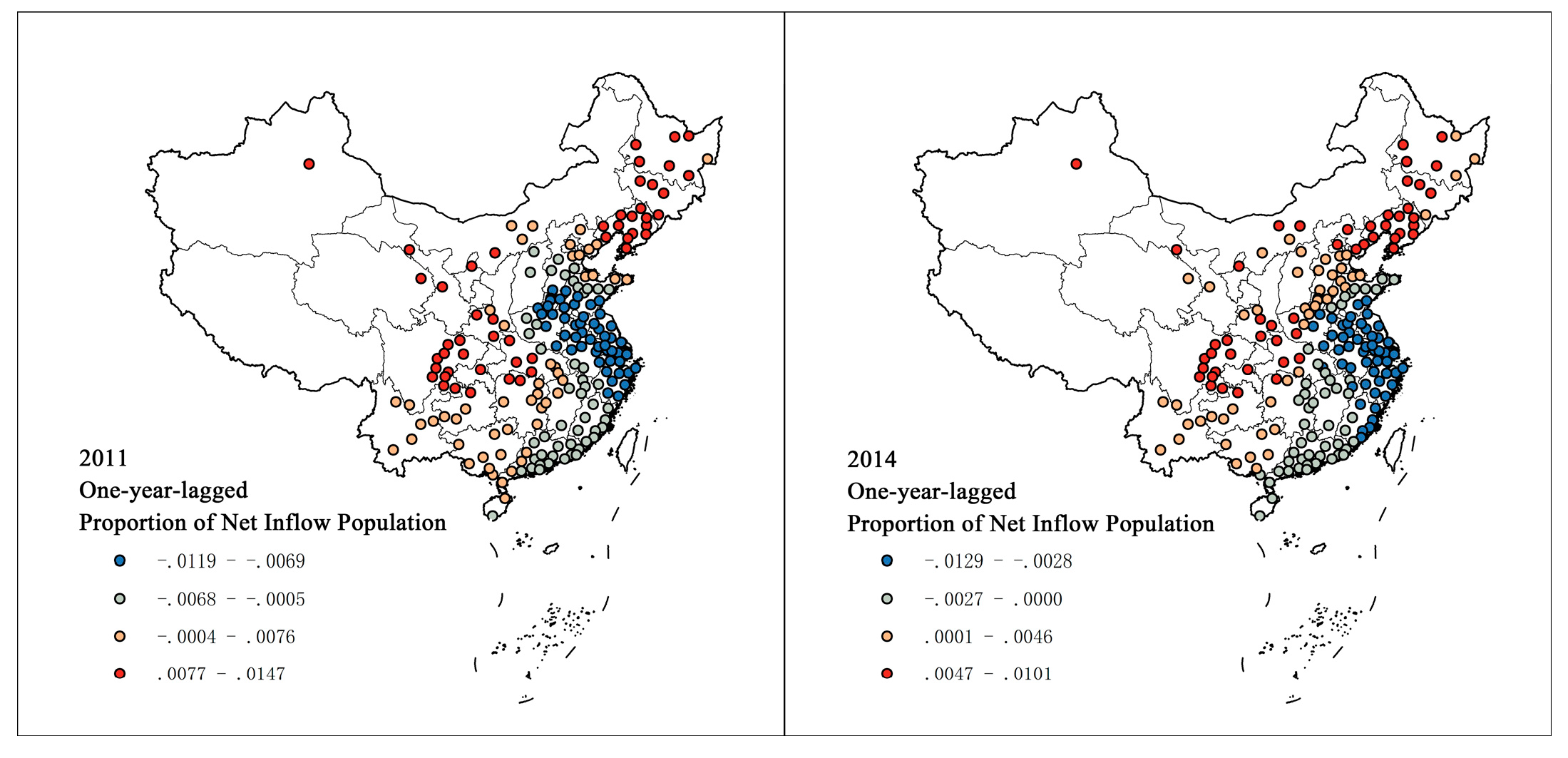
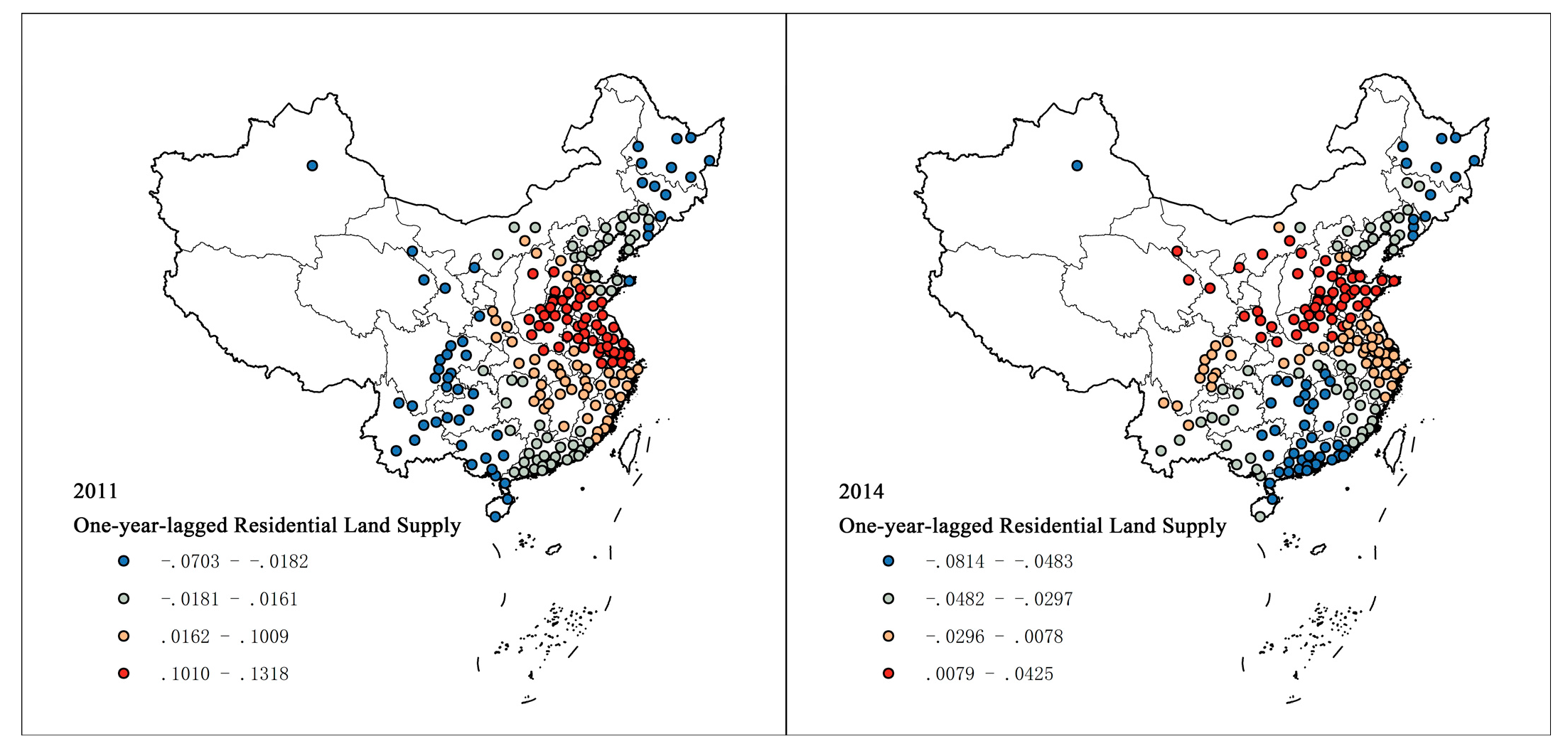
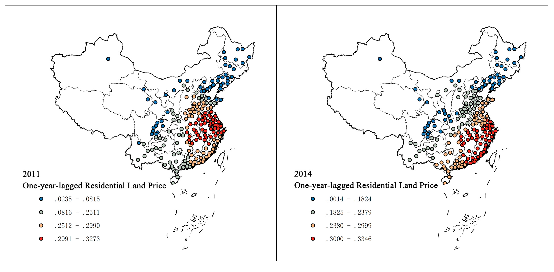
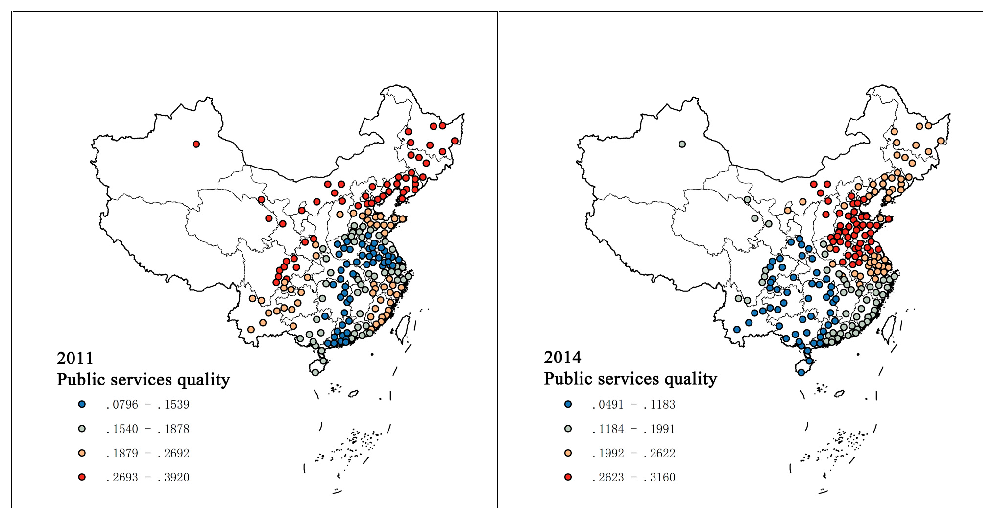
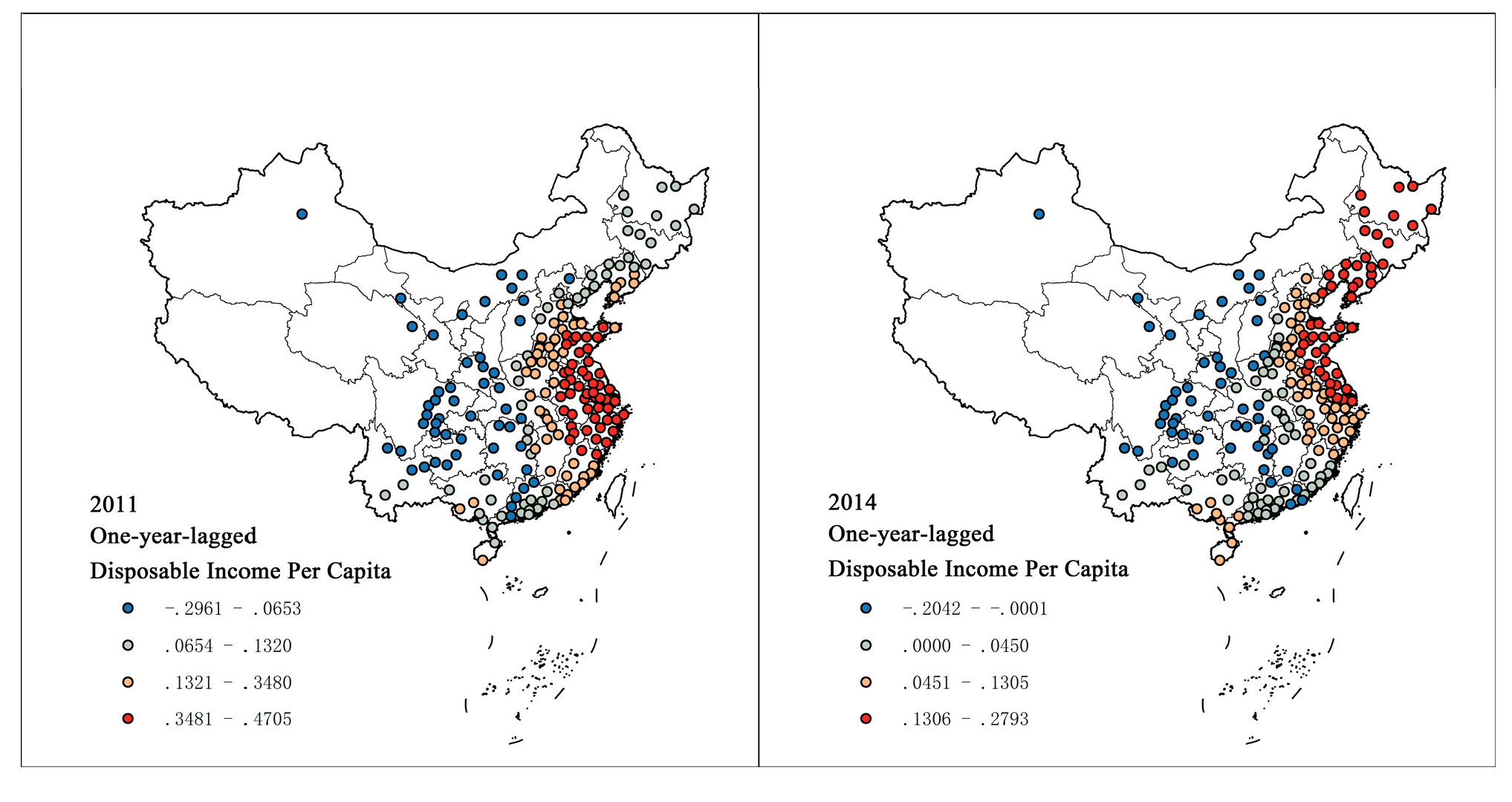
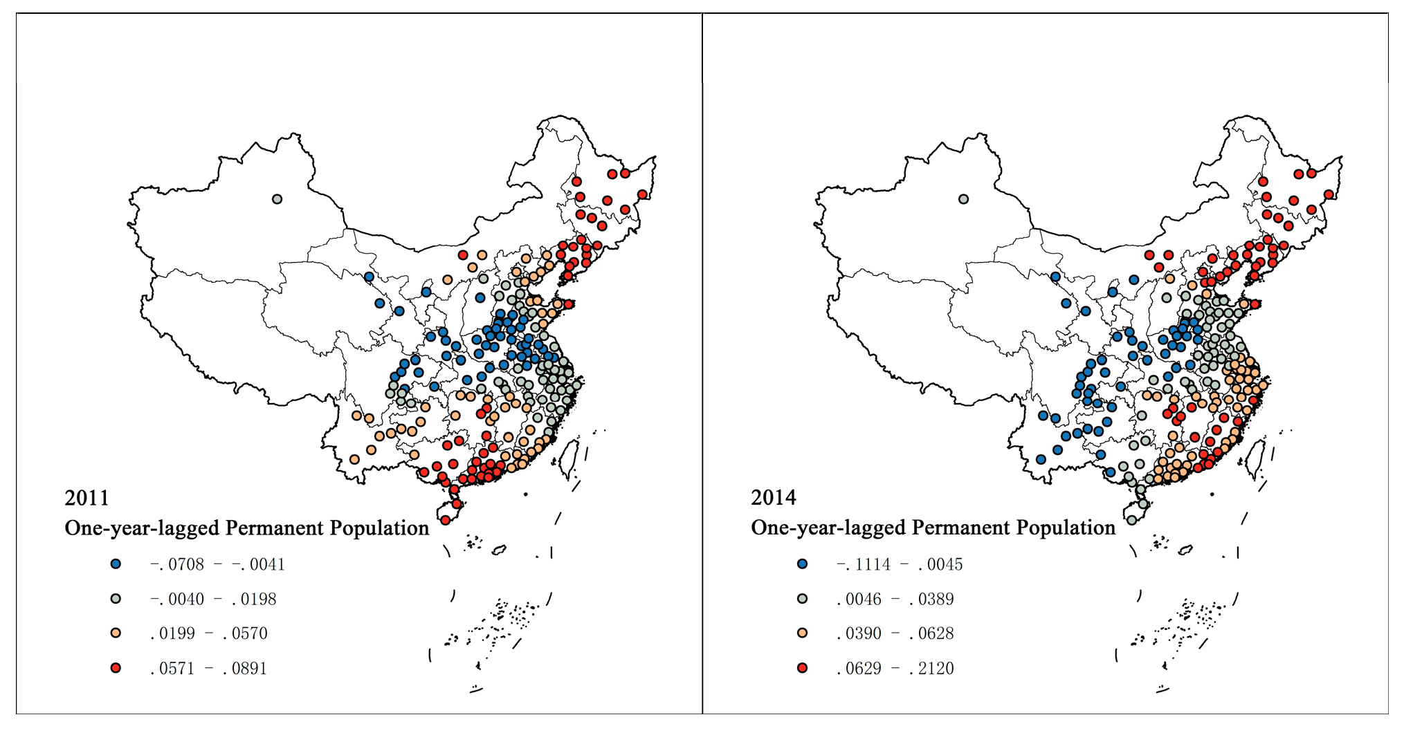
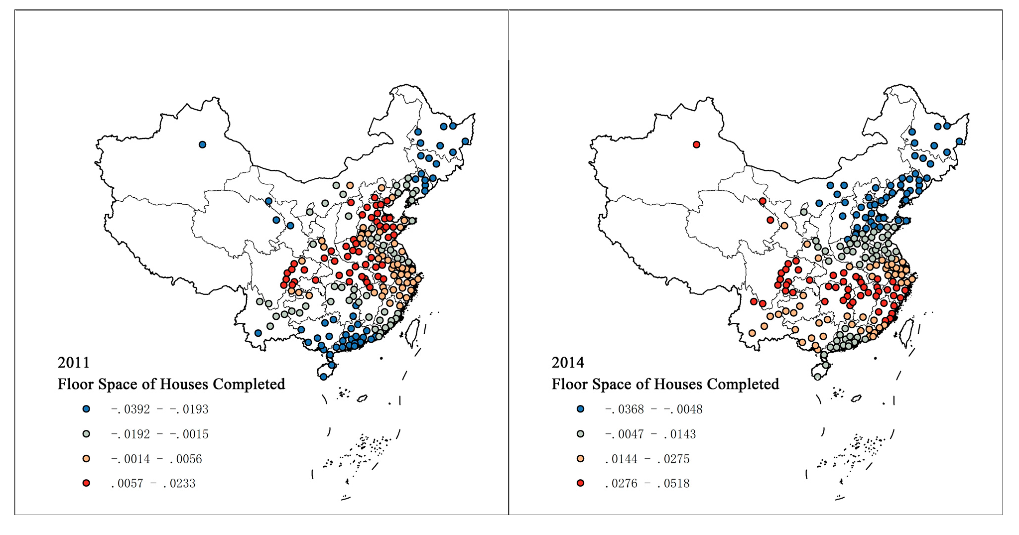
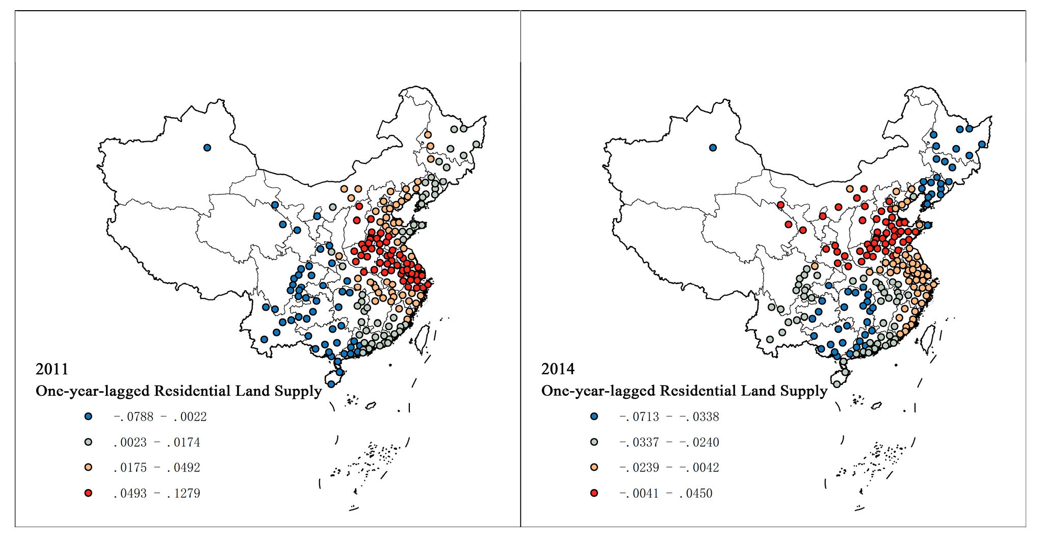
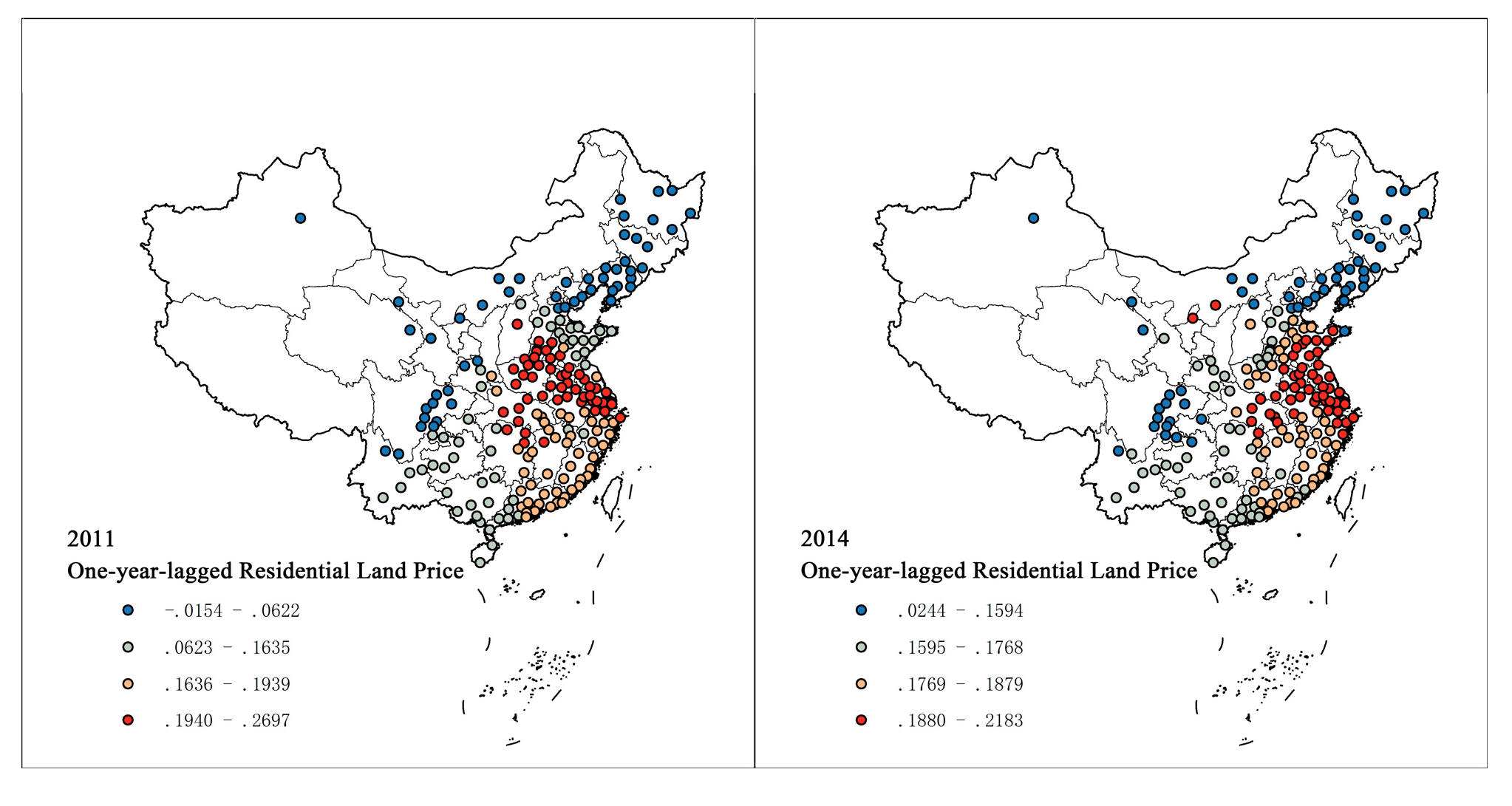
4.2. Spatial and Temporal Variations of the Coefficients

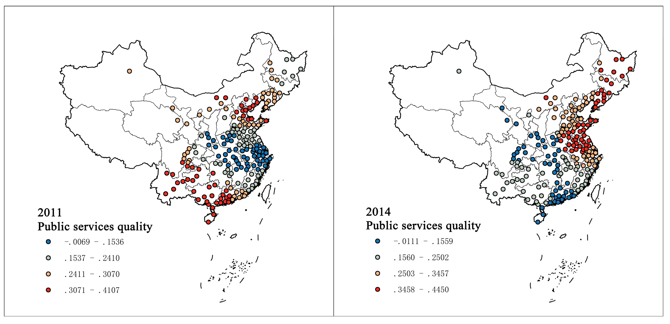
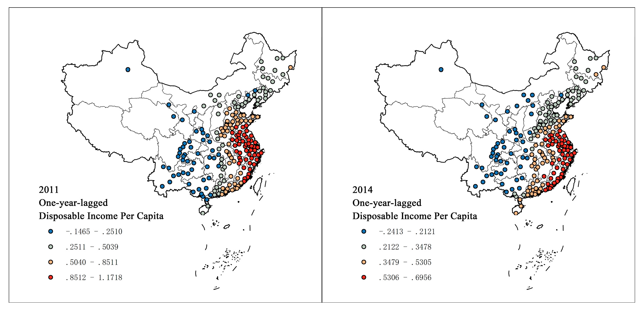
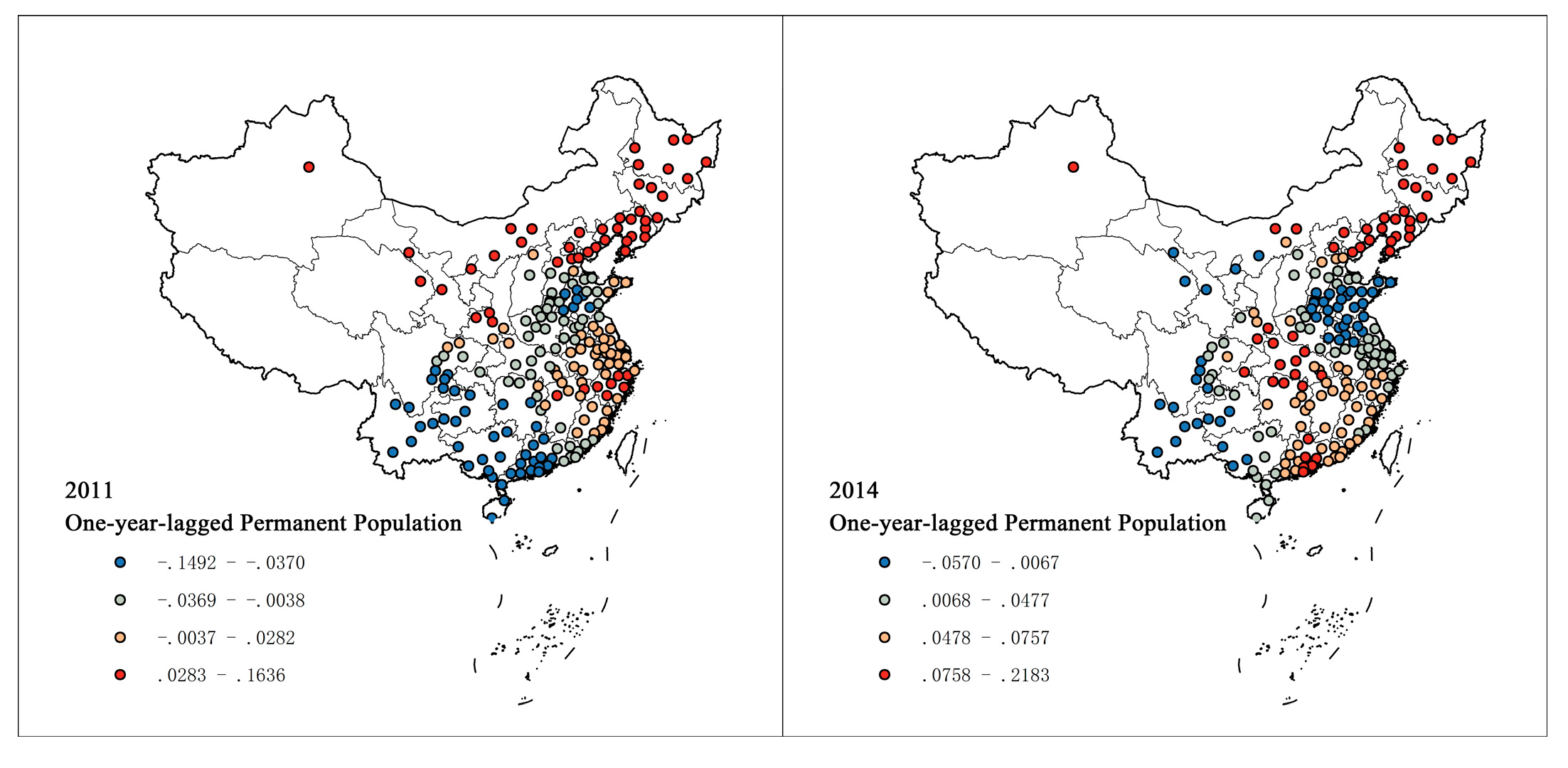
4.2.1. Variables Affecting Housing Prices

To capture the spatial and temporal heterogeneity of the coefficients, the regression results of the GTWR models in years 2011 and 2014 are visualized by ArcGIS. The coefficients of each variable are divided into four quantiles to reflect the degree of influence in the different regions. From red to blue represents the first to fourth quantiles. Due to space limitations, the present study selects the results of some important variables, as shown in Figure 2, Figure 3, Figure 4, Figure 5, Figure 6 and Figure 7. In terms of the demand factors, the positive impact of the public service quality on housing prices in the eastern region is larger, indicating that the public service resources in the eastern region are more limited and the improvement of the public service quality has a greater effect on the housing prices. The per capita disposable income also has a greater impact on housing prices in the eastern coastal areas. It may be because eastern residents generally have more wealth, and the willingness and ability to purchase houses are stronger when disposable income increases. In 2011, the positive impact of the resident population on housing prices in the eastern region was more obvious. In 2014, its positive impact in the eastern region decreased, while its positive impacts in the central and western regions increased. Because the urbanization stage is more advanced in the eastern region, the marginal effects of the resident population on housing prices begins to diminish. In terms of the spatial heterogeneity of net inflow population, a similar pattern can be found. Because the central and western cities are still in the stage of rapid urbanization, the proportion of the net inflow population in the permanent population has a stronger positive effect on housing prices. In terms of supply factors, the supply of residential land in the previous year has a stronger negative effect on housing prices in the eastern and southern region, mainly because residential land in the eastern and southern region is relatively scarce, and the incremental space for residential land is limited. The negative impact of the supply of residential land on housing prices in the eastern and southern region was more obvious in 2014. In terms of development costs, the price of residential land in the previous year has a positive impact on housing prices in most areas, especially in the eastern region. The land cost accounts for a large proportion of China's housing development. The rise in residential land prices not only directly increases housing prices through the cost of housing development in the current period, but will also further push up house prices by affecting expectations. This expectation is more obvious in the eastern region, where residential land resources are relatively limited.

4.2.2. Variables Affecting Housing Rental prices

Using the same method, the spatial and temporal heterogeneity of the coefficient of variables affecting housing rental prices is visualized. Due to space limitations, the results of some important variables are selected to present in this paper (Figure 8, Figure 9, Figure 10, Figure 11, Figure 12 and Figure 13). In terms of the demand factors, public service quality, permanent population, and disposable income have greater positive impacts on the rental prices in the eastern region, indicating that residents in developed areas have higher requirements for public service quality when renting houses, and their ability to pay for rental prices is stronger. However, the mechanism of permanent population on rent is different from that on housing prices. The influence of the permanent population on rental prices is gradually decreasing from the eastern area to the central and western area. It may be because the housing prices in the eastern region are relatively higher, the proportion of the population that rent houses is greater. Therefore, the increase in the same amount of permanent population has a greater positive effect on housing rental prices in the eastern region. In terms of supply factors, the housing stock and supply of residential land in the previous year both have stronger negative impacts on the rental prices in the southern region, mainly due to the relatively limited supply and incremental space of rental housing in the southern areas. The price of residential land in the previous year has a greater positive impact on the rental prices in the coastal and eastern regions. The increases of housing development costs cause housing prices to increase and, thus, lead to higher rental prices. The coefficient has little variation in time, but the spatial variation between coastal and inland areas is always obvious, which indicates that the GTWR model is more favourable than the OLS model.

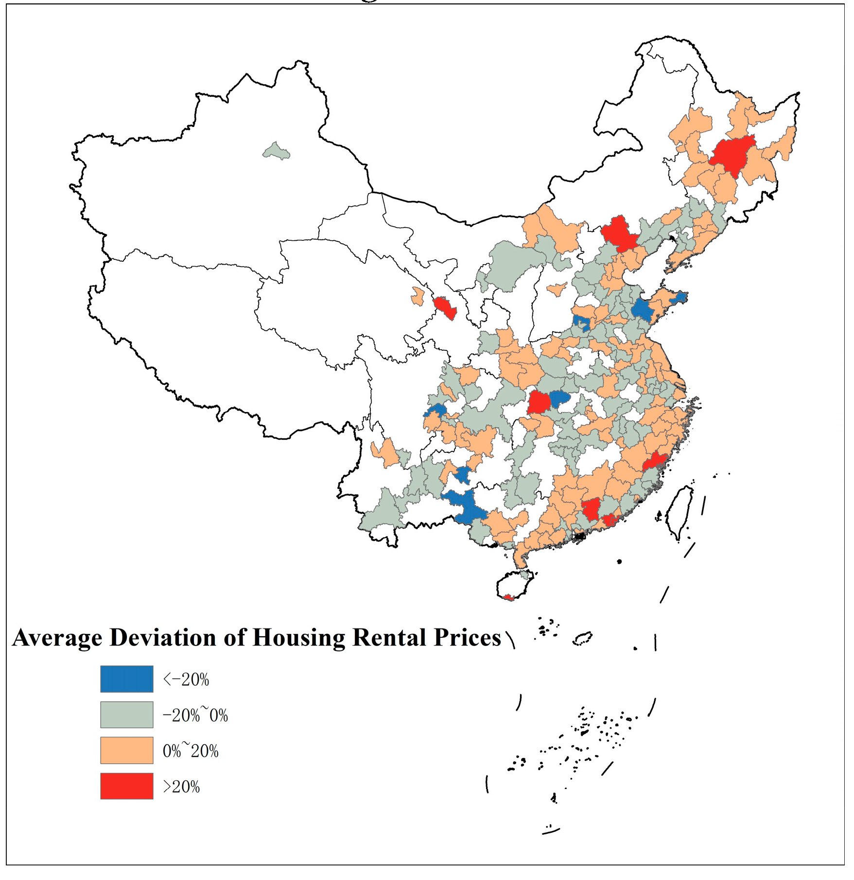
4.3. Analysis of the Spatiotemporal Characteristics of Price Deviations based on the Overall Country

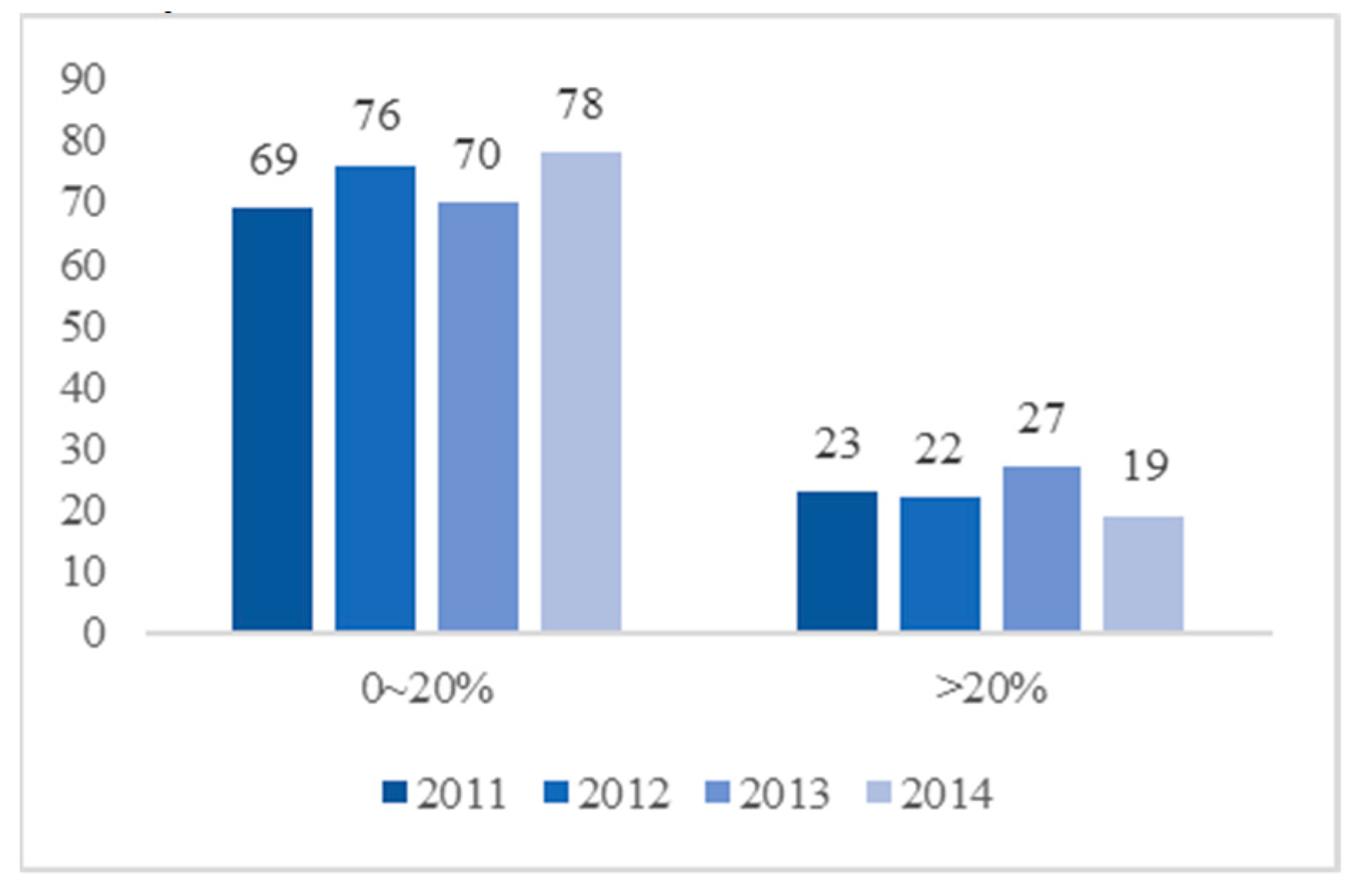
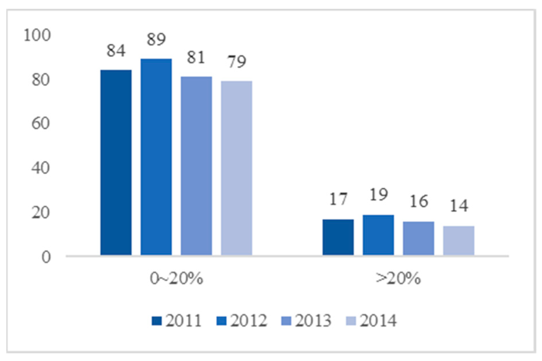
4.3.1. Temporal Variations of Price Deviations

According to the abovementioned housing prices and rental prices model (Equations (5) and (6)), the estimated value of house prices and rental prices determined by the supply–demand in each city is calculated and then compared with the actual value to obtain the price deviation degree. Based on the deviations of house prices and rental prices, cities are divided into two categories, i.e., higher than the estimated value and lower than the estimated value. A degree of deviation greater than 20% is defined as a significant deviation [59].

As seen in Figure 14 and Figure 15, from 2011 to 2014, the number of cities with significant housing price deviations decreased (23 in 2011 and 19 in 2014), indicating that the real estate market regulation implemented in 2010 curbed the excessive growth of housing prices to some extent. The number of cities with significant housing price deviations showed a small rebound only in 2013, when the regulation of the real estate market relaxed slightly. From 2011 to 2014, the number of cities with significant housing rental prices deviations showed a gradual downward trend, reflecting the high correlation between the residential real estate sales and rental markets. Zhang et al. also found that the housing prices in most cities began to return to estimated levels under severe regulatory policies from 2010 to 2011 in their study base on 33 Chinese cities [58].

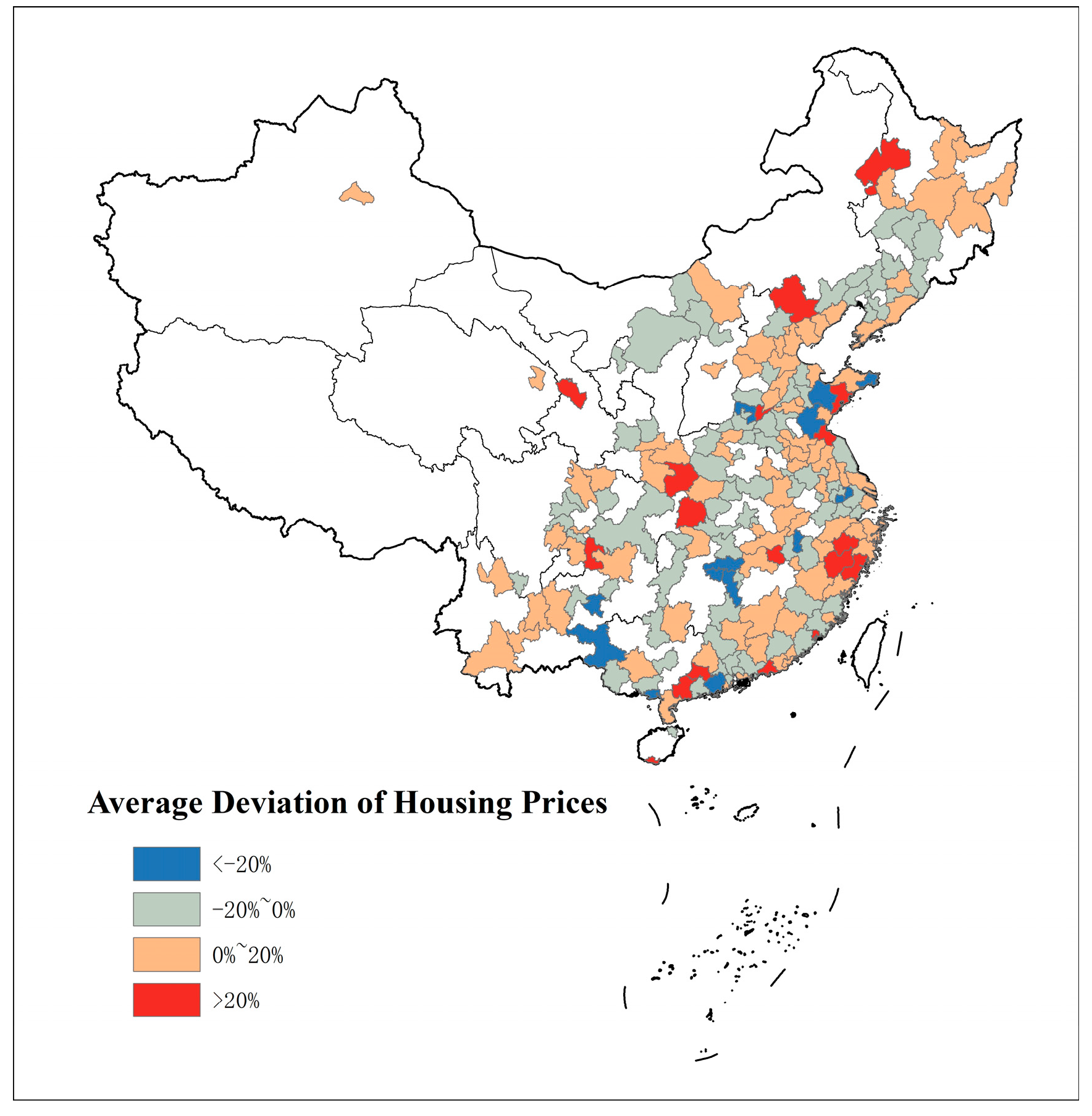
4.3.2. Spatial Characteristics of Price Deviations

To explore the spatial characteristics of housing prices and rental prices deviations, ArcGIS 10.2 is used to visualize the average deviations of housing prices and rental prices in 202 cities during the study period (Figure 16 and Figure 17). The deviation of housing prices and rental prices presents spatial agglomeration in some areas, which is similar to Goodman and Thibodeau's study of the United States [17]. In terms of the average deviation of housing prices, the number of cities with significant deviations is small, which indicates no large-scale housing price bubble. The cities with significant housing price deviations gather in the south-eastern coastal areas, while cities with price deviations between 0% and 20% gather in the Beijing-Tianjin-Hebei City Clusters and north-eastern region. The specific reasons will be discussed later. Judging from the average deviation of rental prices, the number of cities with deviations more than 20% is small, and no spatial aggregation is formed. Cities with rental prices deviations between 0% and 20% form a clear cluster in the south-eastern coastal areas, the Beijing-Tianjin-Hebei City Clusters, and the north-eastern region.

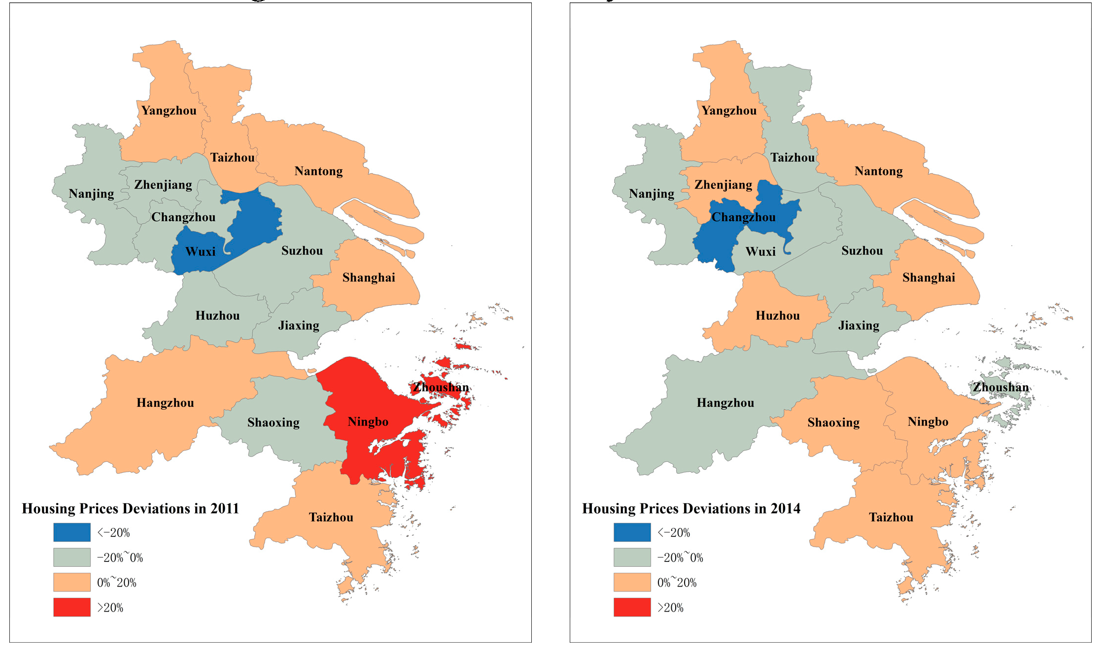
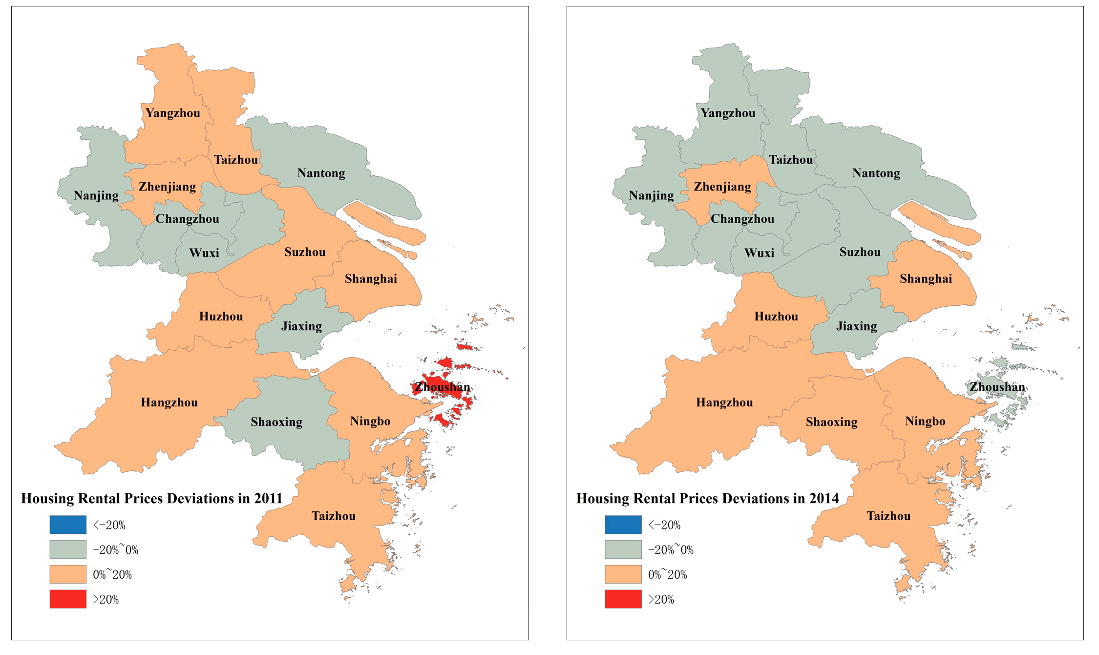
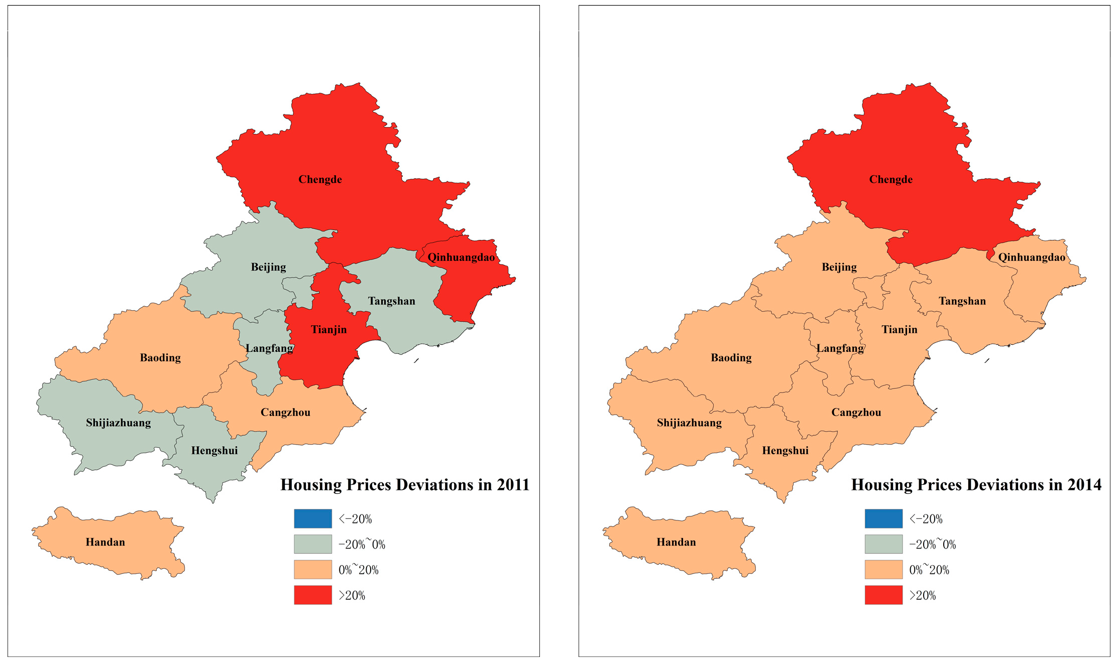
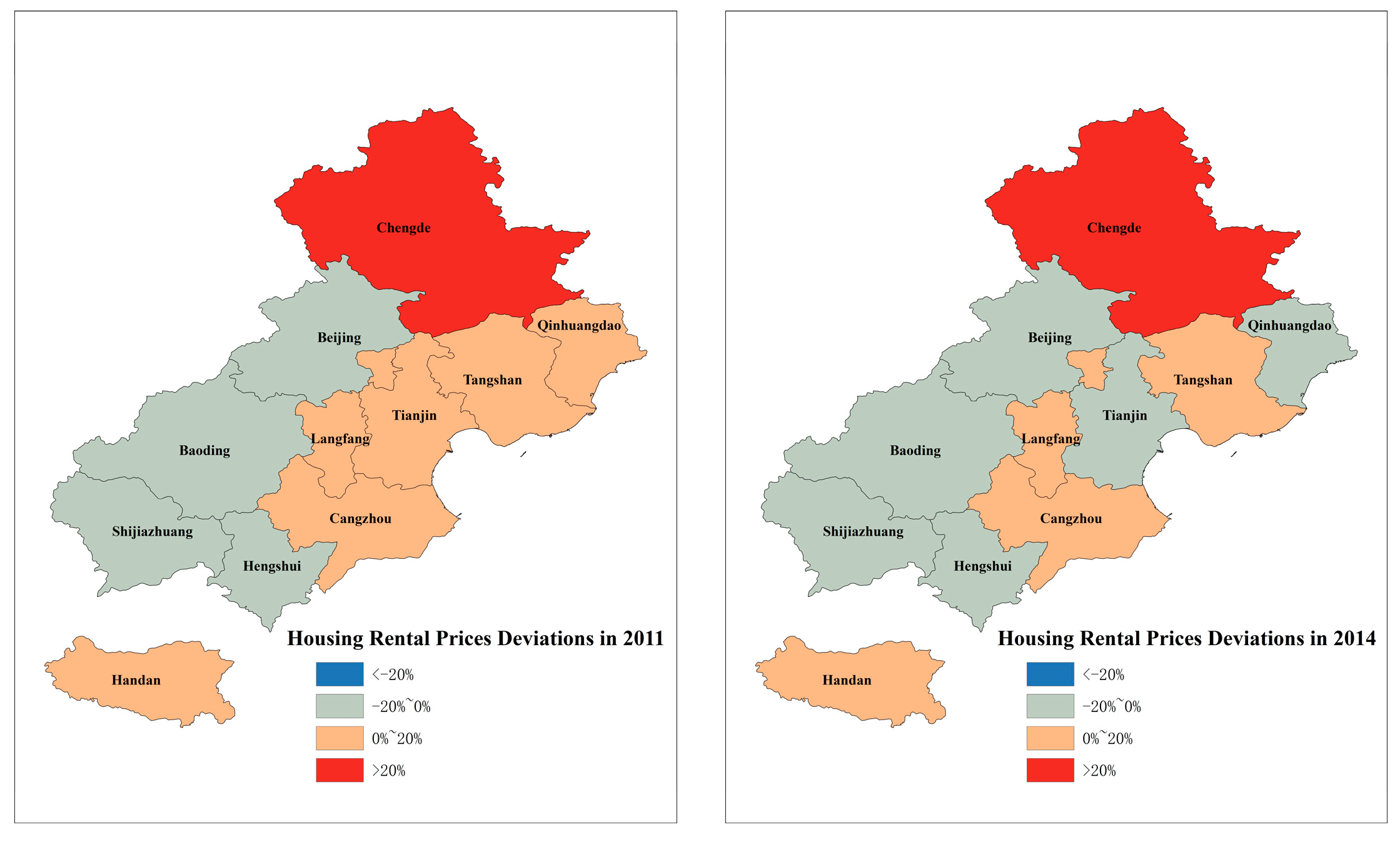
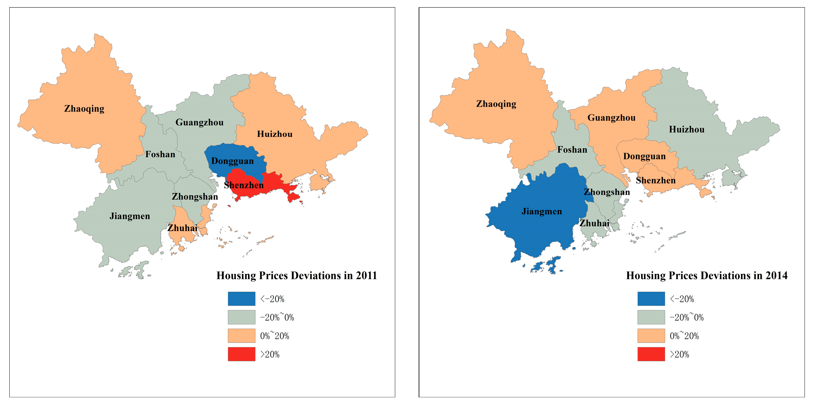
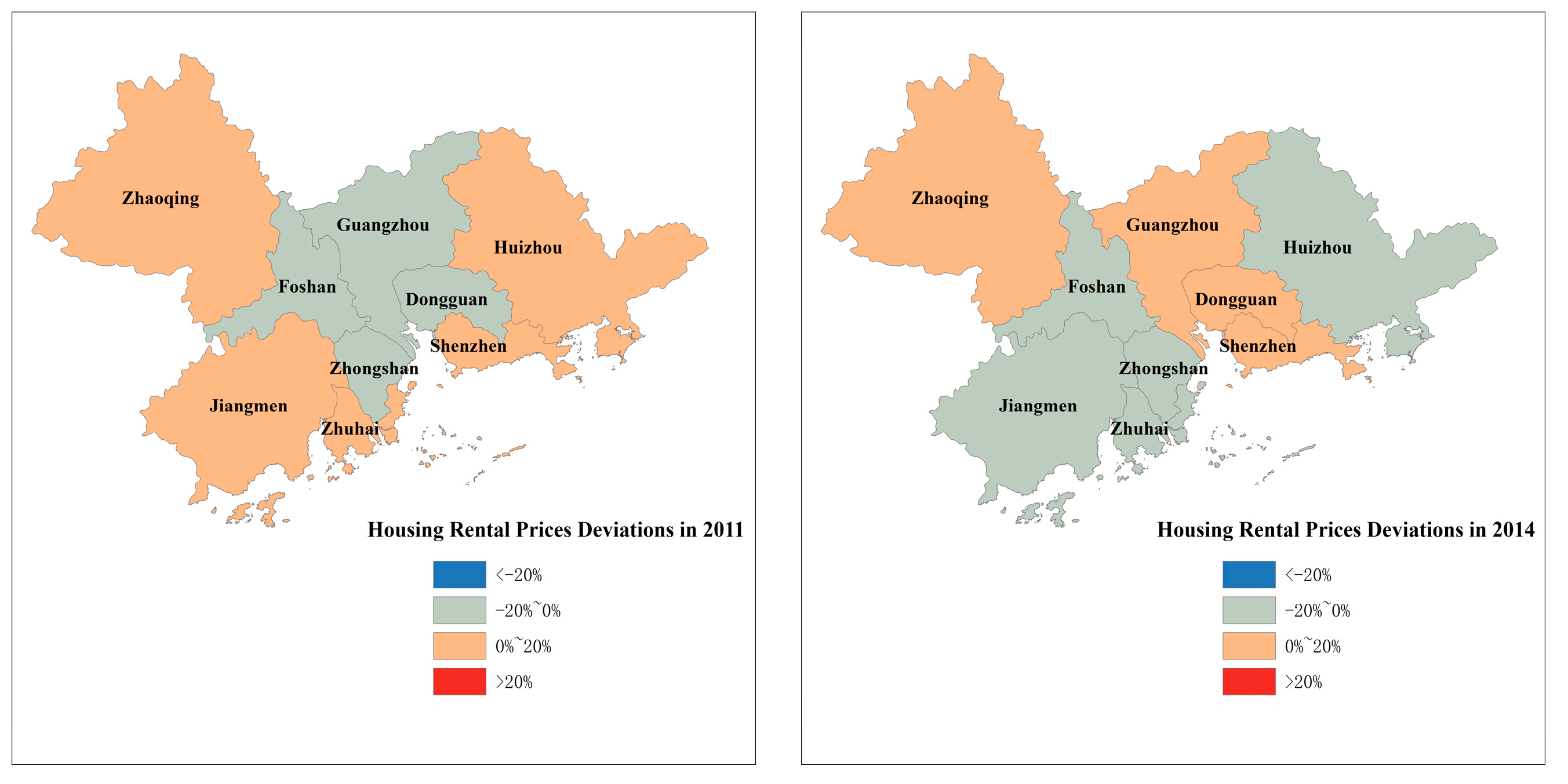
4.4. Analysis of the Spatiotemporal Characteristics of Price Deviations based on Three City Clusters

In the Yangtze River Delta City Cluster, the number of cities where housing prices and rental prices were significantly higher than the estimated value during the sample period decreased. In 2011, the numbers of cities with significant housing prices and rental prices deviations were 2 and 1, respectively, but in 2014, there were no cities with significant housing prices and rental prices deviations. The reason that significant house prices and rental prices deviations in 2011 are more common may be the large increase in the investment demand. The housing demand of the Yangtze River Delta City Cluster is strong, but the land resources are tight, and the housing supply elasticity is small. Many real estate investors are optimistic about the future growth of housing prices and rental prices in the region, resulting in a large influx of demand. In 2014, the prices deviation reductions in most cities in the Yangtze River Delta City Cluster are mainly the result of the continuous growth of the estimated value and the low growth rate of actual value under the control policy. On April 17th, 2010, the State Council issued the Notices on Determination to Inhibit Over Quick Growth of Housing Prices in Some Cities, which inhibits the overly quick growth of housing prices and implements strict differential housing credit policies. Subsequently, hotspot cities released specific purchase and credit limit policies successively, which restricted the number of house purchases and the proportion of down payments. The hotspot cities in Shanghai, Jiangsu Province, and Zhejiang Province in the Yangtze River Delta have all implemented strict purchasing and credit limit policies (shown as Figure 18, Figure 19, Figure 20, Figure 21, Figure 22 and Figure 23). The increase in the estimated value is explained by the rapid economic growth, improvement in the quality of the infrastructure and public services, and a growing permanent population in the Yangtze River Delta City Cluster.

In the Beijing-Tianjin-Hebei City Cluster, it is more common that housing prices and rental prices were higher than the estimated values. In 2011, the housing prices of three cities were significantly higher than the estimated value. The cities with significant deviations decreased in 2014, but the housing prices of the all cities were still higher than the estimated value. The rental prices deviation is similar to that of housing price. It may be related to the expectation regarding the Beijing-Tianjin-Hebei Integration Strategy and insufficient control policies. The Beijing-Tianjin-Hebei Integration Strategy suggests that it is necessary to develop the radioactive driving effect of Beijing, build a world-class City Cluster with Beijing as the core, strengthen industrial synergy within the City Clusters, and further narrow the gap of income and basic public services among cities. Hence, investors have good expectations regarding the housing market in the region, and investment demands began to rush into Beijing and the surrounding cities. Except for the core cities, the Beijing-Tianjin-Hebei City Cluster witnessed overly rapid growth of the actual housing prices because these cities did not implement purchasing and credit limit policies. After the introduction of the Notices on Determination to Inhibit Over Quick Growth of Housing Prices in Some Cities, only Beijing, Tianjin and Shijiazhuang implemented restrictions on the purchases and loans of housing in the Beijing-Tianjin-Hebei Metropolitan Area. The Beijing-Tianjin-Hebei Integrated Strategy advances slowly in the study period and offers limited contributions to the growth of estimated housing prices in the region.

The spatiotemporal characteristics of the housing price and rental prices deviations in the Pearl River Delta City Cluster are different from those in the Yangtze River Delta City Cluster and the Beijing-Tianjin-Hebei City Cluster. In 2011, the number of cities with significant housing price deviations was only one. There were no cities with rental prices significantly higher than the estimated value. Most cities’ housing prices and rental prices were in the normal range. In 2014, the housing prices and rental prices in most cities were undervalued, except for those in the core cities, such as Shenzhen and Guangzhou. As the largest province in China in terms of economic scale, Guangdong Province has long been the destination of population inflow. Although public services and income levels are acceptable in cities other than Guangzhou and Shenzhen, there is still a clear gap between other cities and Guangzhou and Shenzhen. Coupled with the influence of the culture of appreciation for big cities, the core cities attracted most of the demand. In 2014, the housing prices of Guangzhou, Shenzhen, and Dongguan are higher than the estimated value, while the actual demand in other cities is insufficient, leading to housing prices and rental prices that are lower than the estimated value.

5. Conclusions and Implication

5.1. Main Conclusions

The current study first used econometric models to explore determinants of housing prices and rental prices of 202 cities in China and calculate the estimated values of housing prices and rental prices, and then compared estimated values with actual values to calculate deviations. Last, spatiotemporal characteristics of deviations and possible reasons were analysed and discussed. The current study shed some new light on the overall situation of the housing market in large economies, especially with various types of cities, and cities at different stages of development.

First, determinants of urban housing prices and rental prices in China. On the demand side, quality of public services, permanent population size, net inflow of population, and disposal income have significant positive contributions. On the supply side, the housing and land supply have significant negative impacts on housing prices and rental prices, while development costs and land prices have significant positive effects. Rental prices were also positively affected by the previous year's rental yield.

Second, there exists spatial heterogeneity of the above effects, which means the effects of determinants on housing prices and rental prices are stronger in coastal areas than inland areas. Specifically, the positive impacts of public service quality, disposable income, land prices on housing prices and rental prices significantly decline from the east coastal to inland areas in China. Meanwhile, the negative effects of housing stock and land supply reduces from the coastal to inland areas.

Third, the deviation of housing prices and rental prices shows spatial agglomeration in some areas, and the number of cities with significant housing prices and rental prices deviation levels reduced. In China's three most important city clusters, cities with housing prices and rental prices higher than estimated values gathered in the Yangtze River Delta city cluster and Beijing-Tianjin-Hebei city cluster. While the price deviation of most cities in the Pearl River Delta city cluster were relatively moderate. It is worth mentioning that from 2011 to 2014, cities with significant deviations in the Yangtze River Delta and Beijing-Tianjin-Hebei city cluster declined.

5.2. Policy Implications

Based on above conclusions and empirical findings, the current study offers insights for more reasonable public policy in the housing sector. First, housing policies should consider the overall development features in the region. In gathering areas of cities with high housing prices and rents deviations, macro policy’s attention should be focused on the cooperation of different cities’ local policies in the entire region. Meanwhile, detailed policy measures shall be determined according to the specific situation of each city. Second, supply and demand should be considered at the same time as a system. Cities with housing prices and rents higher than the estimated value should strive to improve public service quality and income level, making residents' good expectations for the future a reality. In a word, they should inhibit investment demands and fight for practical actions at the supply side. Third, the new and existing housing market should be considered simultaneously as a whole. Public policies focus on housing purchasing and rent should be simultaneously implemented. If cities face considerable demand pressures and have relatively inadequate stocks, they should exert further efforts to increase the residential land supply and the available house supply. However, given the relative adequate house stocks, policies should pay attention to facilitating a multi-channel house supply, increasing the holding cost of vacant houses, and encouraging house owners to rent vacant houses by providing subsidies. These cities should also consider enhancing the protection of the legal rights of tenants and facilitating the development of the rental housing market.

References

1. Antipa, P.; Lecat, R. The’Housing Bubble’and Financial Factors: Insights from a Structural Model of the French and Spanish Residential Markets. In Housing Markets in Europe; Springer: Berlin, Germany, 2010; pp. 161–186. [Google Scholar]
2. Bucks, B.K.; Kennickell, A.B.; Moore, K.B.; Fries, G.; Neal, A.M. Recent Changes in U.S. Family Finances: Evidence from the 2001 and 2004 Survey of Consumer Finances. Fed. Reserve Bull. 2006, 90, 1–32. [Google Scholar]
3. Manning, C.A. Intercity Differences in Home Price Appreciation. J. Real Estate Res. 1986, 1, 45–46. [Google Scholar]
4. Manning, C.A. Explaining intercity home price differences. J. Real Estate Financ. Econ. 1989, 2, 131–149. [Google Scholar] [CrossRef]
5. Ozanne, L.; Thibodeau, T. Explaining metropolitan housing price differences. J. Urban Econ. 1983, 13, 51–66. [Google Scholar] [CrossRef]
6. Potepan, M.J. Explaining intermetropolitan variation in housing prices, rents and land prices. Real Estate Econ. 1996, 24, 219–245. [Google Scholar] [CrossRef]
7. Fortura, P.; Kushner, J. Canadian InterCity House Price Differentials. Real Estate Econ. 1986, 14, 525–536. [Google Scholar] [CrossRef]
8. Quigley, J.M. Real Estate Prices and Economic Cycles. Int. Real Estate Rev. 1999, 2, 1–20. [Google Scholar]
9. Roback, J. Wages, rents, and the quality of life. J. Political Econ. 1982, 90, 1257–1278. [Google Scholar] [CrossRef]
10. Rosen, S. Wage-based indexes of urban quality of life. Curr. Issues Urban Econ. 1979, 74–104. [Google Scholar]
11. Antoniucci, V.; Marella, G. Housing price gradient and immigrant population: Data from the Italian real estate market. Data Brief 2018, 16, 794–798. [Google Scholar] [CrossRef]
12. Egner, B.; Grabietz, K.J. In search of determinants for quoted housing rents: Empirical evidence from major German cities. Urban Res. Pract. 2018, 11, 460–477. [Google Scholar] [CrossRef] [Green Version]
13. Soo, C.K. Quantifying sentiment with news media across local housing markets. Rev. Financ. Stud. 2018, 31, 3689–3719. [Google Scholar] [CrossRef] [Green Version]
14. Howard, G.; Liebersohn, C. What Explains US House Prices? Regional Income Divergence. In Proceedings of the Regional Income Divergence, 2019 Annual Meeting, St. Louis, MI, USA, 27–29 June 2019; Society for Economic Dynamics: Minneapolis, MN, USA, 2019. [Google Scholar]
15. Abraham, J.M.; Hendershott, P.H. Bubbles in Metropolitan Housing Markets. J. Hous. Res. 1996, 7, 191–207. [Google Scholar]
16. Capozza, D.R.; Hendershott, P.H.; Mack, C. An anatomy of price dynamics in illiquid markets: Analysis and evidence from local housing markets. Real Estate Econ. 2004, 32, 1–32. [Google Scholar] [CrossRef] [Green Version]
17. Goodman, A.C.; Thibodeau, T.G. Where are the speculative bubbles in US housing markets? J. Hous. Econ. 2008, 17, 117–137. [Google Scholar] [CrossRef]
18. Nellis, J.G.; Longbottom, J.A. An empirical analysis of the determination of house prices in the United Kingdom. Urban Stud. 1981, 18, 9–21. [Google Scholar] [CrossRef]
19. Case, K.E.; Shiller, R.J. Is there a bubble in the housing market? Brook. Pap. Econ. Act. 2003, 2003, 299–362. [Google Scholar] [CrossRef] [Green Version]
20. Stiglitz, J.E. Symposium on bubbles. J. Econ. Perspect. 1990, 4, 13–18. [Google Scholar] [CrossRef] [Green Version]
21. Stevenson, S. Modeling housing market fundamentals: Empirical evidence of extreme market conditions. Real Estate Econ. 2008, 36, 1–29. [Google Scholar] [CrossRef]
22. Glaeser, E.L.; Gyourko, J.; Saiz, A. Housing supply and housing bubbles. J. Urban Econ. 2008, 64, 198–217. [Google Scholar] [CrossRef] [Green Version]
23. Mikhed, V.; Zemčík, P. Do house prices reflect fundamentals? Aggregate and panel data evidence. J. Hous. Econ. 2009, 18, 140–149. [Google Scholar] [CrossRef] [Green Version]
24. Malpezzi, S.; Wachter, S. The role of speculation in real estate cycles. J. Real Estate Lit. 2005, 13, 141–164. [Google Scholar] [CrossRef] [Green Version]
25. Dreger, C.; Zhang, Y. Is there a bubble in the Chinese housing market? Urban Policy Res. 2013, 31, 27–39. [Google Scholar] [CrossRef] [Green Version]
26. Li, Q.; Chand, S. House prices and market fundamentals in urban China. Habitat Int. 2013, 40, 148–153. [Google Scholar] [CrossRef]
27. Peng, W.; Tam, D.C.; Yiu, M.S. Property market and the macroeconomy of mainland China: A cross region study. Pac. Econ. Rev. 2008, 13, 240–258. [Google Scholar] [CrossRef]
28. Wang, Z.; Zhang, Q. Fundamental factors in the housing markets of China. J. Hous. Econ. 2014, 25, 53–61. [Google Scholar] [CrossRef]
29. Wu, J.; Gyourko, J.; Deng, Y. Evaluating the risk of Chinese housing markets: What we know and what we need to know. China Econ. Rev. 2016, 39, 91–114. [Google Scholar] [CrossRef] [Green Version]
30. Yu, H. China’s house price: Affected by economic fundamentals or real estate policy? Front. Econ. China 2010, 5, 25–51. [Google Scholar] [CrossRef]
31. Yue, S.; Hongyu, L. Housing Prices and Economic Fundamentals: A Cross City Analysis of China for 1995—2002. Econ. Res. J. 2004, 6, 78–86. [Google Scholar]
32. Yunfang, L.; Tiemei, G. Empirical Analysis on Real Estate Price Fluctuation in Different Provinces of China. Econ. Res. J. 2007, 8, 133–142. [Google Scholar]
33. Huang, B.; Wu, B.; Barry, M. Geographically and temporally weighted regression for modeling spatio-temporal variation in house prices. Int. J. Geogr. Inf. Sci. 2010, 24, 383–401. [Google Scholar] [CrossRef]
34. Oikarinen, E.; Engblom, J. Differences in housing price dynamics across cities: A comparison of different panel model specifications. Urban Stud. 2016, 53, 2312–2329. [Google Scholar] [CrossRef]
35. Wang, S.; Wang, J.; Wang, Y. Effect of land prices on the spatial differentiation of housing prices: Evidence from cross-county analyses in China. J. Geogr. Sci. 2018, 28, 725–740. [Google Scholar] [CrossRef] [Green Version]
36. Stewart Fotheringham, A.; Charlton, M.; Brunsdon, C. The geography of parameter space: An investigation of spatial non-stationarity. Int. J. Geogr. Inf. Syst. 1996, 10, 605–627. [Google Scholar] [CrossRef]
37. Bitter, C.; Mulligan, G.F.; Dall’erba, S. Incorporating spatial variation in housing attribute prices: A comparison of geographically weighted regression and the spatial expansion method. J. Geogr. Syst. 2007, 9, 7–27. [Google Scholar] [CrossRef] [Green Version]
38. Mou, Y.; He, Q.; Zhou, B. Detecting the spatially non-stationary relationships between housing price and its determinants in China: Guide for housing market sustainability. Sustainability 2017, 9, 1826. [Google Scholar] [CrossRef] [Green Version]
39. Cai, R.; Yu, D.; Oppenheimer, M. Estimating the Effects of Weather Variations on Corn Yields Using Geographically Weighted Panel Regression. In Proceedings of the 2012 Annual Meeting, Seattle, WA, USA, 12–14 August 2012; Agricultural and Applied Economics Association: Milwaukee, WI, USA, 2012. [Google Scholar]
40. Yu, D. Exploring spatiotemporally varying regressed relationships: The geographically weighted panel regression analysis. Int. Arch. Photogramm. Remote Sens. Spat. Inf. Sci. 2010, 38, 134–139. [Google Scholar]
41. Tabak, B.M.; Miranda, R.B.; Fazio, D.M. A geographically weighted approach to measuring efficiency in panel data: The case of US saving banks. J. Bank. Financ. 2013, 37, 3747–3756. [Google Scholar] [CrossRef]
42. Páez, A.; Uchida, T.; Miyamoto, K. A general framework for estimation and inference of geographically weighted regression models: 1. Location-specific kernel bandwidths and a test for locational heterogeneity. Environ. Plan. A 2002, 34, 733–754. [Google Scholar] [CrossRef]
43. Mussa, A.; Nwaogu, U.G.; Pozo, S. Immigration and housing: A spatial econometric analysis. J. Hous. Econ. 2017, 35, 13–25. [Google Scholar] [CrossRef]
44. Saiz, A. Immigration and housing rents in American cities. J. Urban Econ. 2007, 61, 345–371. [Google Scholar] [CrossRef] [Green Version]
45. Wang, Y.; Wang, S.; Li, G.; Zhang, H.; Jin, L.; Su, Y.; Wu, K. Identifying the determinants of housing prices in China using spatial regression and the geographical detector technique. Appl. Geogr. 2017, 79, 26–36. [Google Scholar] [CrossRef]
46. Chau, K.W.; Chin, T. A critical review of literature on the hedonic price model. Int. J. Hous. Sci. Its Appl. 2003, 27, 145–165. [Google Scholar]
47. Gibbons, S.; Machin, S. Valuing school quality, better transport, and lower crime: Evidence from house prices. Oxf. Rev. Econ. Policy 2008, 24, 99–119. [Google Scholar] [CrossRef]
48. Jim, C.Y.; Chen, W.Y. External effects of neighbourhood parks and landscape elements on high-rise residential value. Land Use Policy 2010, 27, 662–670. [Google Scholar] [CrossRef]
49. Nguyen-Hoang, P.; Yinger, J. The capitalization of school quality into house values: A review. J. Hous. Econ. 2011, 20, 30–48. [Google Scholar] [CrossRef]
50. Zheng, S.; Hu, W.; Wang, R. How much is a good school worth in Beijing? Identifying price premium with paired resale and rental data. J. Real Estate Financ. Econ. 2016, 53, 184–199. [Google Scholar] [CrossRef]
51. Feng, H.; Lu, M. School quality and housing prices: Empirical evidence from a natural experiment in Shanghai, China. J. Hous. Econ. 2013, 22, 291–307. [Google Scholar] [CrossRef]
52. Wen, H.; Xiao, Y.; Hui, E.C.; Zhang, L. Education quality, accessibility, and housing price: Does spatial heterogeneity exist in education capitalization? Habitat Int. 2018, 78, 68–82. [Google Scholar] [CrossRef]
53. Wen, H.; Xiao, Y.; Zhang, L. School district, education quality, and housing price: Evidence from a natural experiment in Hangzhou, China. Cities 2017, 66, 72–80. [Google Scholar] [CrossRef]
54. Hwang, M.; Quigley, J.M. Economic fundamentals in local housing markets: Evidence from US metropolitan regions. J. Reg. Sci. 2006, 46, 425–453. [Google Scholar] [CrossRef] [Green Version]
55. Glaeser, E.L.; Gyourko, J.; Saks, R.E. Urban growth and housing supply. J. Econ. Geogr. 2005, 6, 71–89. [Google Scholar] [CrossRef] [Green Version]
56. Mayer, C.J.; Somerville, C.T. Land use regulation and new construction. Reg. Sci. Urban Econ. 2000, 30, 639–662. [Google Scholar] [CrossRef]
57. Pollakowski, H.O.; Wachter, S.M. The effects of land-use constraints on housing prices. Land Econ. 1990, 66, 315–324. [Google Scholar] [CrossRef]
58. Zhang, D.; Liu, Z.; Fan, G.-Z.; Horsewood, N. Price bubbles and policy interventions in the Chinese housing market. J. Hous. Built Environ. 2017, 32, 133–155. [Google Scholar] [CrossRef]
59. Oikarinen, E.; Bourassa, S.C.; Hoesli, M.; Engblom, J. US metropolitan house price dynamics. J. Urban Econ. 2018, 105, 54–69. [Google Scholar] [CrossRef]
Figure 1. Research Process.
Sustainability 11 07232 g001
Figure 2. Spatiotemporal variations of PSQ.
Sustainability 11 07232 g002
Figure 3. Spatiotemporal variations of one-year-lagged disposable income per capita.
Sustainability 11 07232 g003
Figure 4. Spatiotemporal variations of one-year-lagged permanent population.
Sustainability 11 07232 g004
Figure 5. Spatiotemporal variations of one-year-lagged proportion of net inflow population.
Sustainability 11 07232 g005
Figure 6. Spatiotemporal variations of residential land supply.
Sustainability 11 07232 g006
Figure 7. Spatiotemporal variations of residential land price.
Sustainability 11 07232 g007
Figure 8. Spatiotemporal variations of PSQ.
Sustainability 11 07232 g008
Figure 9. Spatiotemporal variations of disposable income per capita.
Sustainability 11 07232 g009
Figure 10. Spatiotemporal variations of permanent population.
Sustainability 11 07232 g010
Figure 11. Spatiotemporal variations of floor space of houses completed.
Sustainability 11 07232 g011
Figure 12. Spatiotemporal variations of residential land supply.
Sustainability 11 07232 g012
Figure 13. Spatiotemporal variations of residential land price.
Sustainability 11 07232 g013
Figure 14. The number of cities with significant housing price deviations.
Sustainability 11 07232 g014
Figure 15. The number of cities with significant housing rental prices deviations.
Sustainability 11 07232 g015
Figure 16. Average deviation of housing prices.
Sustainability 11 07232 g016
Figure 17. Average deviation of housing rental prices.
Sustainability 11 07232 g017
Figure 18. Housing prices deviations in the Yangtze River Delta City Cluster.
Sustainability 11 07232 g018
Figure 19. Housing rental prices deviations in the Yangtze River Delta City Cluster.
Sustainability 11 07232 g019
Figure 20. Housing prices deviations in the Beijing-Tianjin-Hebei City Cluster.
Sustainability 11 07232 g020
Figure 21. Housing rental prices deviations in the Beijing-Tianjin-Hebei City Cluster.
Sustainability 11 07232 g021
Figure 22. Housing prices deviations in the Pearl River Delta City Cluster.
Sustainability 11 07232 g022
Figure 23. Housing rental prices deviations in the Pearl River Delta City Cluster.
Sustainability 11 07232 g023