A Hybrid Unequal Clustering Based on Density with Energy Conservation in Wireless Nodes

Abstract

The Internet of things (IoT) provides the possibility of communication between smart devices and any object at any time. In this context, wireless nodes play an important role in reducing costs and simple use. Since these nodes are often used in less accessible locations, recharging their battery is hardly feasible and in some cases is practically impossible. Hence, energy conservation within each node is a challenging discussion. Clustering is an efficient solution to increase the lifetime of the network and reduce the energy consumption of the nodes. In this paper, a novel hybrid unequal multi-hop clustering based on density (HCD) is proposed to increase the network lifetime. In the proposed protocol, the cluster head (CH) selection is performed only by comparing the status of each node to its neighboring nodes. In this new technique, the parameters involving energy of nodes, the number of neighboring nodes, the distance to the base station (BS), and the layer where the node is placed in are considered in CH selection. So, in this new and simple technique considers energy consumption of the network and load balancing. Clustering is performed unequally so that cluster heads (CHs) close to BS have more energy for data relay. Also, a hybrid dynamic–static clustering was performed to decrease overhead. In the current protocol, a distributed clustering and multi-hop routing approach was applied between cluster members (CMs), to CHs, and CHs to BS. HCD is applied as a novel assistance to cluster heads (ACHs) mechanism, in a way that a CH accepts to use member nodes with suitable state to share traffic load. Furthermore, we performed simulation for two different scenarios. Simulation results showed the reliability of the proposed method as it was resulted in a significant increase in network stability and energy balance as well as network lifetime and efficiency.

1. Introduction

The Internet of Things (IoT) is based on the fact that each object or thing can use wireless communication to communicate with each other [1]. Nowadays, IoT has attracted attentions of societies, governments, and industries for a wide range of applications including smart homes, healthcare services, environmental monitoring, smart transportation, smart networks, security, fire detection, finance tracking, smart lighting, etc. [2].

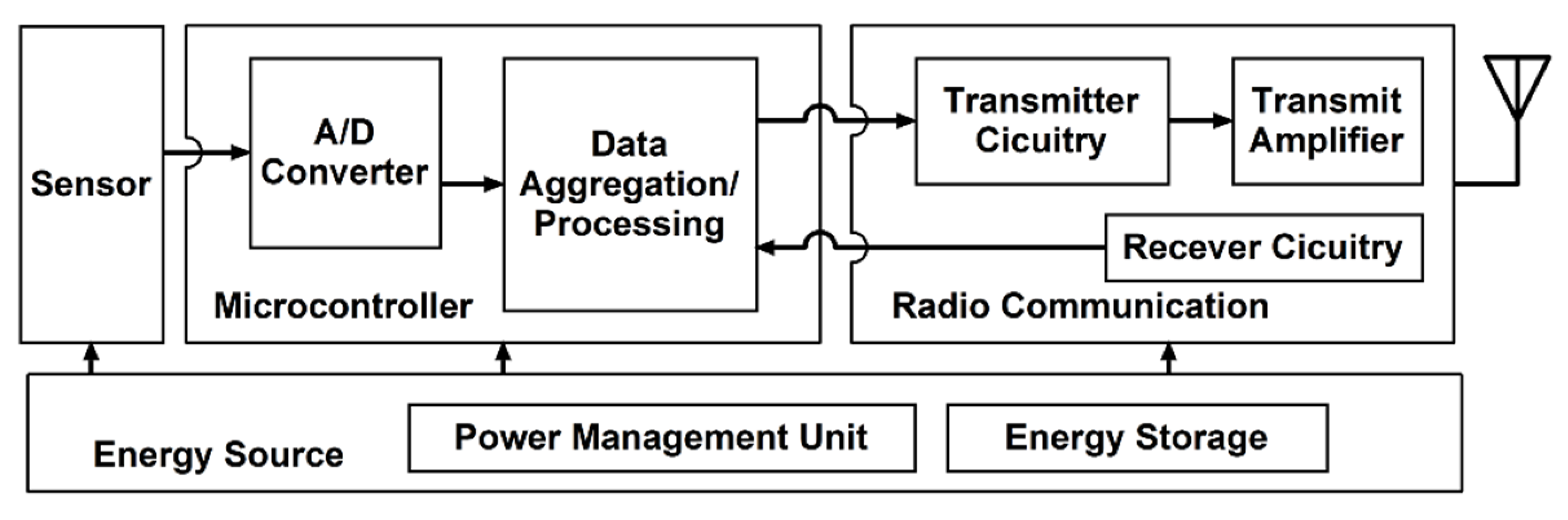
In this context, wireless sensor networks (WSNs) play an important role in increasing the number of networks with low-cost smart devices which can be easily installed. WSNs are widely-used in various fields such as environment, health, military etc. Each node is composed of a sensor unit, processing unit (microcontroller), the radio communication unit, and an energy resource. Figure 1 represents these components. Examples include wildlife and environment supervision, health monitory, pediment supervision, border supervision and control, security, etc. [3,4,5].

Wireless nodes typically have capabilities such as sensing, computing and self-organizing operations for routing and data transmission to a base station (BS) [6]. However, limitations of wireless nodes include short-range communications, low bandwidth, processing/storage limitation and, particularly, energy consumption [7]. One of the main problems in IoT based on wireless nodes is the energy consumption in nodes. Each node has a battery and therefore, limited energy is stored in it. Since the implemented wireless nodes are not easily accessible, it is hardly possible to access the nodes and recharge or exchange the battery. Energy consumption mainly occurs in sensing, data processing, and data transmission [7]. However, most of the mentioned energy consumption is related to data transmission. Therefore, reducing energy consumption in these networks is an ongoing research [8,9].

Routing between two nodes with the highest energy efficiency and balanced energy consumption between them are two of the factors that can affect the lifetime of a network significantly. One of the methods to reduce energy consumption in these networks is to find an optimal route by applying to cluster [7,9,10].

In the clustering method, nodes are divided into clusters and one node within a cluster is selected as a cluster head (CH). The cluster member (CMs) nodes, sensing the environment, send the data to the CH. The CH receives data from CMs and aggregates them and finally; the aggregated data is transferred directly or indirectly to a BS with the help of middle nodes. In fact, the purpose of clustering is to find an optimal route to send data to a BS [11].

Clustering protocols are usually classified into two protocols including static and dynamic protocols. In static protocols, clustering is performed once and the nodes always remain in the same cluster. Virtual concentric circle band-based clustering (VCCBC) [12] and an energy-efficient protocol with static clustering (EEPSC) [13] are two of the examples of the static clustering methods in WSNs; although, in terms purely of static protocol performance, network overhead is reduced but shows instability for a long period of time. The main disadvantage of static methods is that it results in energy depletion in several nodes [14,15]. In dynamic protocols, clustering is performed in each round, and new clusters form during each round. Low-energy adaptive clustering hierarchy (LEACH) [3] is one of the examples of the dynamic clustering methods. Dynamic performance can improve network lifetime, but usually, it has a high overhead [14,15].

Clustering is the most important energy efficient technique. In this technique, the sensor nodes are organized into groups termed as clusters. The regular nodes in the cluster are called as cluster members and a CH is selected among them [16,17]. In order to prevent the network from hot spot issue, unequal clustering techniques can be utilized for load balancing between the CHs [18,19].

Recently, hybrid static–dynamic methods have been proposed for clustering. Hybrid unequal clustering with layering protocol (HUCL) [15] is one of the examples of these clustering methods. This method is a hybrid of both static and dynamic clustering. Therefore, similar to dynamic protocols, this method performs clustering during each round and, as per static protocols, the clusters remain the same during several rounds. Within each cluster, a node is assigned as CH and remains the same until another node is selected as the new CH. After some rounds, clustering and cluster formation are performed again. This procedure always continues in the lifetime of a network. In the hybrid method, the overhead can be reduced in addition to improvement of network stability and lifetime [14,15].

Furthermore, the clustering protocols and CH selection methods in wireless nodes are typically divided into two categories: centralized and distributed clustering [10,14]. In the centralized clustering method, the BS uses the general knowledge of a network for clustering the nodes and a BS needs to collect the information about the status of the nodes within a network for clustering the nodes. This method is not applicable to large-scale networks [14]. In the distributed method, nodes perform routing in a self-organized manner and without requiring more information about the network position. In distributed algorithms, each node decides about its own CH probability based on some parameters [10]. In these algorithms, a BS has no effect on the CH selection. In contrast to centralized clustering, distributed methods are more efficient for large-scale networks. Therefore, there is less overhead in these methods due to the omission of messages transferred between nodes and a BS [14].

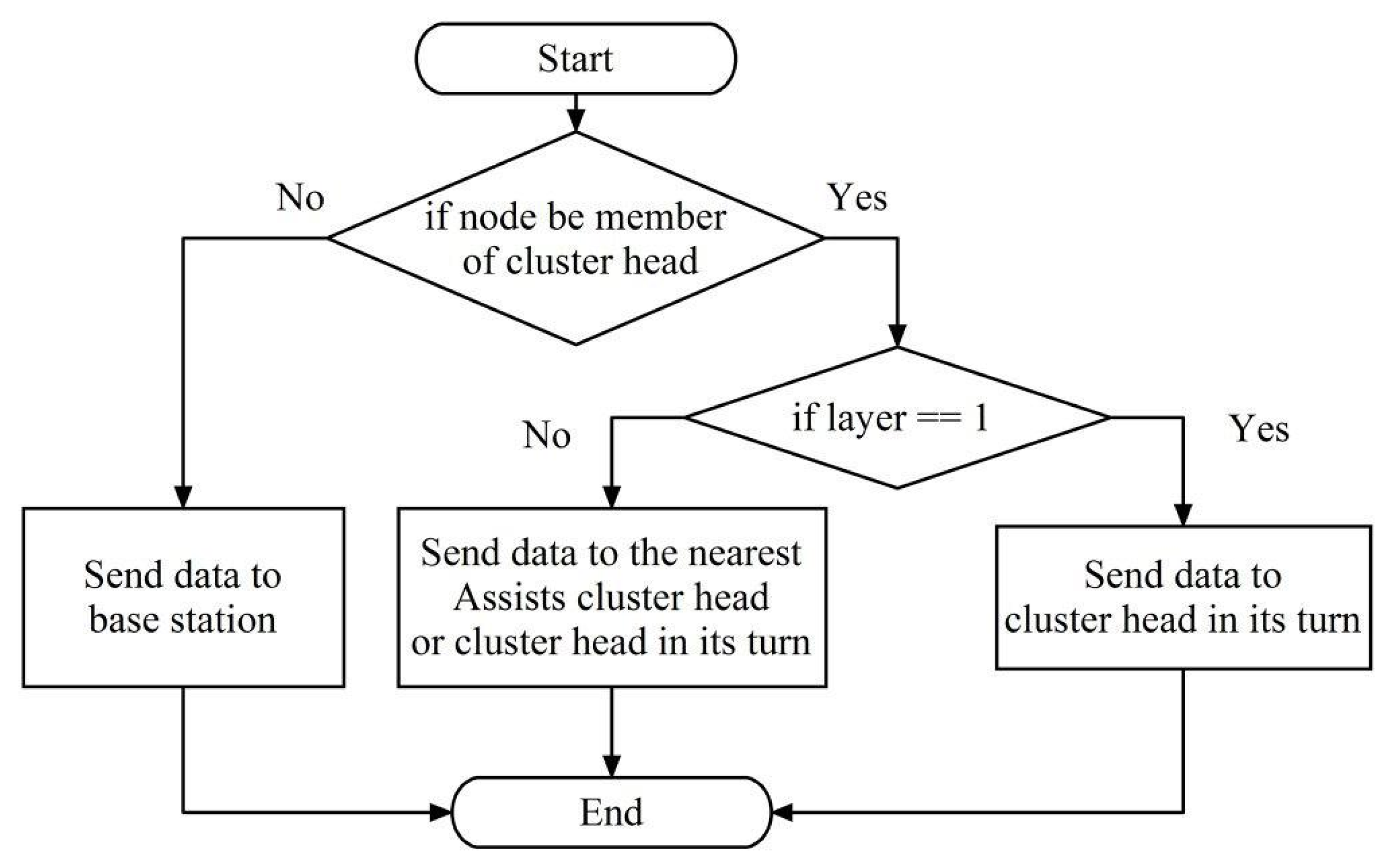
In this paper, given the above-mentioned advantages, the performance of a novel hybrid static–dynamic protocol is used. The current paper places emphasis on a distributed clustering algorithm. The probability of selecting a node as a CH is determined on the basis of energy level, a number of neighbors and distance to BS within each sensor and its neighbors. Moreover, CMs send a data packet to CH based on assistance to cluster heads (ACHs) mechanism and CH send packages to a BS through an energy-aware multi-hop routing method. Clustering is performed unequally. In this clustering, CHs close to the BS have smaller radius; as a result, the number of CMs are reduced and less energy is consumed for receiving data. In this way, they spend more energy to receive data from CHs far from the BS.

The remainder of this paper is organized as follows. A literature review is presented in Section 2. Section 3 gives our proposed algorithm in detail. Analysis of our proposed HCD algorithm is further discussed in Section 4. In Section 5, extensive evaluation and simulation results are given with discussion and analysis and Section 6 concludes this paper.

2. Literature Review

In the last decades, extensive research has been carried out around wireless nodes clustering. Some studies were performed on the basis of centralized clustering whilst some others presented a distributed clustering method.

A subset of widely-used clustering algorithms could be mentioned as LEACH, LEACH-centralized (LEACH-C) [3], and hybrid energy-efficient distributed clustering (HEED) [20].

One of the main distributed clustering algorithms used to reduce energy consumption in WSNs is the LEACH algorithm. In this algorithm, CH is selected based on a random rotation. Therefore, the energy consumption has been optimized and the energy load in distributed throughout the network. If fixed nodes are selected as CH, their energy will end soon, and they die earlier than other nodes. Hence, nodes are selected as a CH by a fixed probability, and they introduce themselves to the whole network. Since CH is selected in a probable manner, it is possible that they are close to each other; therefore, one of LEACH problems is the heterogeneous distribution of CH in the environment.

Another widely-used algorithm proposed is the HEED algorithm [20]. In this algorithm, each node creates a random number between zero and one. If a number smaller than CH probability is selected for the node, that node is then selected as tentative CH. If CH is equal to one, then the node becomes the final CH. Otherwise, the tentative CH remains, and finally, CH probability becomes doubled. In each ordinary node, if the CH probe is equal to one, then the node becomes final CH. Otherwise, it creates a random number between zero and one. If the number is smaller than CH probability, the node is then selected as a tentative CH, and finally, CH probability becomes double. This procedure continues until CH is selected. CH is selected according to the remaining energy of the node and they are considered as the second parameter of communication costs inside the cluster. Collectively, nodes join a CH whose distance to the related CH is smaller.

Another distributed clustering algorithm is density and distance based CH selection algorithm (DDCHS) [21]. In the clustering step, the area is virtually divided into hexagons so that circular cluster overlap is prevented and in fact, some borders are considered for clusters. For each hexagon, a CH is selected and subsequently, some subcircles are taken into account in the virtual hexagons according to the average of usual nodes distances to the cluster center. This algorithm is composed of three steps: (i) local grouping which determines a center in length and width of the clustering area. The area is divided into four equal parts, (ii) comparison of nodes density—the node density is determined in each part and one of the parts is selected as a candidate quarter. (iii) Comparing the distance between nodes by computing the distance of each node to other available nodes in candidate quarter and selecting the node with the shortest distance to other nodes as a CH.

An energy-aware distributed dynamic clustering protocol, based on fuzzy logic (ECPF) [22], is another algorithm introduced in 2012. This method performed the clustering by using the fuzzy logic and taking the energy of nodes as a nonprobabilistic parameter. The node selection was done sporadically. This protocol reduced the overhead of the network, by providing the mechanism similar to a setup phase, rather than performing the setup phase in each round. With regard to energy saving, the purpose of this algorithm was to select a set of appropriate clusters which covers the whole region selection by means of a fuzzy system. So in this fuzzy system, input parameters such as the degree and the center of the nodes were considered. The use of fuzzy logic in selecting the CH and the rule of overhead reduction contributed to improving the lifetime of the network. One of the challenges proposed in this clustering is the lack of complete coverage in the network in the time range.

Other solutions, such as energy-based clustering for WSNs lifetime optimization and balancing energy consumption in clustered WSNs (BLAC), were proposed by Ducrocq et al. [23]. BLAC used the energy level and the degree of nodes or the density of nodes for clustering. The protocol performs as distributed and dynamic. BLAC balanced the energy consumption between nodes and improved the network lifetime and stability. In order to balance the energy, the CH rotates between nodes. These methods involve overload.

Energy and coverage-aware distributed clustering (ECDC) protocol [24] was proposed in 2014. The protocol was based on two components: energy and coverage. In this protocol, nodes share their information with their neighbors for calculating a delay time. According to the calculated delay time, CH is elected to the network. ECDC protocol was able to improve the coverage. Thus, the aforementioned protocol contributed to decreased energy consumption and increased the lifespan of the network. However, this method is carried out dynamically and it involves higher overload.

Hybrid unequal clustering with layering protocol (HUCL) was presented in 2015 [15]. HUCL is a hybrid of dynamic and static clustering methods. Clusters closer to the BS were smaller. In this method, CHs are selected based on the energy status of the node, the distance to a BS and the number of neighbors. Also, data is transferred to the BS as multihops. Each node shared its own information with the size of its cluster reduces for neighbors. In the HUCL method, each node computes its own delay time and CH are selected according to the computed delay times and, therefore, the nodes join to the nearest CH. In this algorithm the CH that has no member node changes its own state to a member node and finally, it joins to the nearest CH. Data transmission step is divided into time periods. Member nodes send their own data clusters to CH and CH use multihop routing to transmit data to the BS. Simulation results show that compared to other available protocols, HUCL is able to reduce the network overhead, optimize energy consumption, and increase the network lifetime. In this algorithm, in order to compute the cluster radius, energy consumption of nodes, and also for calculation delay time, a distance of a node to BS is not taken into account.

An improved energy aware distributed unequal clustering protocol (EADUC-II) was proposed in 2016 [25]. In this method, clusters are formed with unequal sizes and thus, clusters near to a BS have a smaller size. To determine the competition radius of cluster nodes, other parameters have been considered including node energy and to determine routing, the criterion of node energy to select the next step is taken into account for routing between CH. In this method, in order to compute the node delay time and node density, its distance to the BS is not considered. Although this method is performed in hybrid form, the improvement of overload reduction is less.

Another algorithm is an unequal multi-hop balanced immune clustering protocol (UMBIC) which was proposed in 2016 [26]. In multi-hop routing, the CH which is near to the BS loses its energy due to the relay data of the further CH. This protocol provided the WSNs with the nodes of various sizes and with a variety of homogeneous and heterogeneous nodes with distinctive densities; therefore, this method resulted in an improved network lifetime. UMBIC used an unequal clustering method to optimize the energy consumption in intra- and intercluster routing, forming the unequal clusters based on the distance of a node to BS and the energy level of the node. Also, UMBIC used the multi-objective immune algorithm to provide the routing tree with the aim of minimizing the cost of the nodes’ relationship. Hence, this method could effectively reduce the network overhead and improve network lifetime.

A grid-based reliable routing protocol (GBRR) was proposed in 2016 [27]. This protocol improves the quality of the communication within the intracluster and intercluster by creating virtual clusters based on square grids and proper selection of the steps. This protocol divided the network into equally square-shaped grids so that in each grid one or more nodes might exist. According to the local information of the nodes’ condition and grids, clustering was performed in a way that one cluster can occupy one or more grid. To reduce the overhead of CH, the multihop routing algorithm calculated the most efficient route between clusters; therefore, the source node does not need to transmit the data through the middle CHs to BS. In CH Competition stage of this method, it can be improved by considering the node’s distance to the BS.

An energy-efficient QoS routing for WSNs using a self-stabilizing algorithm was proposed in 2015 [28]. This paper presented a self-stabilizing hop-constrained energy-efficient (SHE) clustering and a multi-hop routing algorithm for declining the delay and improving the quality of packet transmission. This protocol performs as a hybrid clustering method. CHs are determined by the BS in a definitive and offline Method and routing is done as distributed and online. The advantage of this protocol is that clustering is initialized only once at the beginning of the network. This protocol is based on TDMA schedules using the clustering algorithm for transmitting the data within the cluster in a manner that the nodes of the cluster with a tolerable delay send their own data to CH. Also, an adaptable routing protocol was proposed for data transmission between CH and the BS.

Chanak et al. [29] proposed an energy-aware distributed routing algorithm to tolerate network failure in WSNs. This protocol has specific routing schemes for better tolerating the network failure in the current position. This scheme includes three new algorithms. In a distributed energy-efficient heterogeneous clustering (DEEHC) network clustering is done according to the residual energy in order to minimize the energy required for data transmission. During clustering, each sensor node finds k-vertex disjoint paths for sending data to the CH according to the energy levels of neighbor nodes. In other words, the routing between nodes CH and BS is done based on the proposed k-vertex disjoint path routing (KVDPR) algorithm. In addition, the route maintenance mechanism (RMM) algorithm enables nodes and CH to keep a route, which is based on the neighbor nodes energy conditions and prevents failure. In DEEHC algorithm, for determining CH using computing time, distance to the BS, and node density are not considered.

Naeem et al. [30] proposed a dynamic and cooperative clustering. Furthermore, a new technique called the neighborhood formation scheme is presented. This algorithm aims to distribute energy demand among nodes and optimize a number of sensors involved in detection and report of events. This algorithm is executed distributed and dynamically. Results show that the proposed framework improved network lifetime and reliability in data transmission.

An energy-aware multi-hop routing (EAMR) protocol was proposed in 2017 [31]. This method aims to reduce overhead by reducing variations of CHs. In this method, a method similar to LEACH [3] is sued to select initial CHs to form clusters. EAMR allows a node to operate as a cluster head until its energy is not lower than a threshold; therefore, in this algorithm, CHs vary only when required. In order to improve network lifetime, this algorithm employs multi-hop routing. However, since membership of nodes in a cluster does not change until the end, in selecting the initial CHs, many of the important parameters like nodes density and distance from BS is not considered.

To sum up, the above section has summarized some clustering protocols which were provided to increase wireless node lifetime and that also reviewed recent hybrid methods to reduce the overhead and increase the lifetime of wireless nodes.

Table 1. Comparison of some of the clustering algorithms.

Protocol	Cluster Size	Intracom.	Intercom.	Method	CH Election	Dynamism
LEACH [3]	equal	1-hop	1-hop	distributed	Random	dynamic
LEACH-C [3]	equal	1-hop	1-hop	centralized	deterministic by BS	dynamic
HEED [20]	equal	1-hop	k-hop	distributed	hybrid, based on Attribute	dynamic
DDCHS [21]	equal	1-hop	1-hop	distributed	based on density & distance	dynamic
VCCBC [12]	equal	1-hop	k-hop	distributed	CH rotation	static
EEPSC [13]	equal	1-hop	1-hop	distributed	selection by previous CH	static
ECPF [22]	equal	1-hop	k-hop	distributed	based on fuzzy logic	dynamic
BLAC [23]	equal	1-hop	k-hop	distributed	based on energy & degree or density	dynamic
ECDC [24]	equal	1-hop	k-hop	distributed	based on energy & coverage	dynamic
SHE [28]	equal	1-hop	k-hop	centralized	deterministic by BS	dynamic
HUCL [15]	unequal	1-hop	k-hop	distributed	hybrid, based on attribute	hybrid
GBRR [27]	equal	1-hop	k-hop	distributed	based on grid structure	dynamic
DEEHC [29]	equal	k-hop	k-hop	distributed	based on energy	dynamic
EADUC-II [25]	unequal	1-hop	k-hop	distributed	hybrid, based on attribute	hybrid
UDSC [30]	equal	1-hop	k-hop	distributed	hybrid, based on Attribute	dynamic
EMAR [31]	equal	1-hop	k-hop	distributed	at first random, then CH rotation	static
proposed alg.	unequal	k-hop	k-hop	distributed	hybrid, based on density	hybrid

shows a summary and comparison of some of the clustering algorithms.

The proposed protocol is an improvement of the HUCL protocol and the method is reviewed in the following sections. This improvement is due to the fact that in our protocol is a novel hybrid unequal clustering which is performed by a simple efficient algorithm for selecting CH node based on density, energy level, and distance to the BS. It also proposed a new mechanism by assisting the CH with intracluster data transmission as well as improved intercluster data transmission using layered mechanism. The main objective is to provide a high-precision clustering protocol to balance the energy consumption, decrease the overhead, substantial increase of networks’ lifetime, and finally, to improve existing methods.

3. The Proposed HCD Algorithm

In this section, we introduce a hybrid unequal multi-hop clustering based on density (HCD) to improve network lifetime and throughput. HCD is performed by the distributed method. In this method, clustering is performed as a hybrid of static and dynamic methods. We assumed that nodes can detect their own distance by received signal strength indicator (RSSI) and considered CH relation according to the energy level and nodes situation in the network. Since the CH node consumes more energy, it is prevented to select the nodes having no desirable energy status as a CH and, therefore, the network stability increases. Also, the energy-aware multi-hop method was used for routing between CH.

3.1. Network Model

An IoT based on wireless nodes and a BS with an unlimited power supply connected to the network are the primary considerations in our model. Data is sampled by sensor nodes and they are routed in order to be sent to the BS. Also, each node can perform as a CH or non-CH node. Some assumptions of the network model are as follows.

• N wireless nodes are randomly distributed in M*M environment.
• Nodes are heterogeneous.
• All nodes and the BS are fixed.
• All nodes can set transfer power in terms of the distance between nodes.
• CH can aggregate data.

The first order radio model of energy consumption in this proposed method is similar to the LEACH protocol [3]. Energy consumption transfer is defined as Equation (1).

$$E_{TX}(i,K,d_{ij})=\{\begin{array}{c}\begin{array}{ccc}{E}_{elec}K+E_{fs}K{d}_{ij}{}^2& & \begin{array}{cc}if& d_{ij}\le d_o\end{array}\end{array}\\ \begin{array}{ccc}{E}_{elec}K+E_{mp}K{d}_{ij}{}^4& & \begin{array}{cc}if& d_{ij}>d_o\end{array}\end{array}\end{array}$$

(1)

where K is the number of data bits and d_ij is the distance between two nodes—i and j. E_elec is energy consumption in sender or receiver circuit to send a data bit. E_fs and E_mp are energy consumptions in the sender amplifier for sending a data bit in terms of distance between the receiver and sender. Also, d₀ value, which is a threshold distance, is obtained from Equation (2).

$$d_0=\sqrt{\frac{E_{fs}}{E_{mp}}}$$

(2)

In an energy model, a receiver energy consumption is defined as Equation (3).

$$E_{RX}(i,K)=E_{elec}K$$

(3)

According to the data aggregation model used in our simulation, it is assumed that the information collected by a set of N nodes can be packed in a k bit package.

3.2. Protocol Performance

After deploying nodes, a layering stage is performed. Each of the nodes computes its distance from the BS. For calculating this distance, the BS broadcast a signal which will be heard by all nodes and each node approximates its own calculated distance to the BS using the RSSI. Consequently, the node informs its position to the BS. The BS then starts layering the network. In the beginning, the BS calculates the difference between the closest and the furthest nodes to itself and experimentally defines four layers for networks. The BS sends messages within the network and assigns layer ID for each node.

All HCD operations are involved in cluster initialization stage and data transmission stage. Cluster initialization stage is composed of four phases including the delay time calculation phase, CH selection phase, cluster formation phase, and route construction phase. The data transmission stage is divided into a number of major slots. Each major slot is formed by several rounds and two substages which are called CH rotation and adjustment route. Each round involves in intercluster transmission phase and intracluster transmission phase. In a CH rotation, the role of CH is to turn between member nodes to prevent discharging of the energy in CH. The operation of HCD is displayed in Figure 2. Figure 3 also shows the flowchart of the proposed algorithm.

3.2.1. Cluster Initialization

In this stage, network nodes are divided into groups to form clusters. In the first phase, when the network is operational, the probability of each node to become a CH and its cluster radius are determined based on the energy level of the node and its distance to the BS. Nodes calculate their own cluster radius according to Equation (4).

$$R_c(i)=\left[1-\alpha (\frac{d_{BS,\max }-d_{i,BS}}{d_{BS,\max }-d_{BS,\min }})-\beta (1-\frac{E_{rem}(i,r)}{E_{Max}})\right]R{L}_{\max }\times \lambda$$

(4)

In the above-mentioned Equation, R_c(i) is the radius of node i and RL_max is maximum competition radius for being a CH, as determined previously. E_rem(i,r) is the remaining energy of the node i in the round r and E_max stands for the maximum energy capacity of the node. d_BS,max and d_BS,min are the maximum and minimum distance of nodes from the BS and d_i,BS is the distance of i_th node from the BS. α and β are also weight factors that can vary between zero and one. λ is the weight factor associated with the layer where the nodes are located. In the lower layers RL_max is multiplied by a smaller coefficient to the nodes which are closer to the BS and, thus, has a smaller radius. In contrast, further clusters are multiplied by a greater coefficient to have a larger radius. Accordingly, if a node is selected as a CH it will have more energy to receive and transmit the data than the further CH to the BS.

Before computing delay time, each node shares its location information and energy level with its neighbors. All nodes, which are situated in its radio range, receive the node’s message from all neighbors. After informing the nodes of their neighbors, they are able to calculate the average energy of neighbor’s nodes which is calculated using Equation (5).

$$E_{Ave}(i,r)=\frac{{\displaystyle \sum _{j\in N_{\mathit{nbr}}(i,r)}{E}_{rem}(j,r)}}{\max (\left|N_{\mathit{nbr}}(i,r)\right|,\epsilon )}$$

(5)

N_nbr(i,r) is the number of sets of nodes of neighbors i in the round of r. |N_nbr(i,r)| is node degree or number of neighbors for node i in the round r. The parameter ε is a very small number in order to avoid infinity caused by division by zero. Each node will give itself a scoring point parameter in order to start the routine of becoming a CH based on density. In the first cluster initialization stage, the point of CH for each node is zero. Each node considers its neighbors and if the energy level of the neighbor is smaller than its own energy level, it increases its point by one unit. The scoring point needed for each node to become a CH is updated after the computation given in Equation (6).

$$\begin{array}{l}\begin{array}{cc}\forall & j\in N_{nbr}(i,r)\end{array}\\ if\begin{array}{cc}& E_{rem}(i,r)>E_{rem}(j,r)\begin{array}{cc}& then\begin{array}{cc}& p(i)=p(i)+1\end{array}\end{array}\end{array}\\ if\begin{array}{cc}& |N_{nbr}(i,r)|>|N_{nbr}(j,r)|\begin{array}{cc}& then\begin{array}{cc}& p(i)=p(i)+1\end{array}\end{array}\end{array}\\ if\begin{array}{cc}& i{d}_{Layer}(i)<i{d}_{Layer}(j)\begin{array}{cc}& then\begin{array}{cc}& p(i)=p(i)+1\end{array}\end{array}\end{array}\\ if\begin{array}{cc}& d_{i,BS}<d_{j,BS}\begin{array}{cc}& then\begin{array}{cc}& p(i)=p(i)+1\end{array}\end{array}\end{array}\end{array}$$

(6)

P is the score point given to nodes. id_Layer(i) is the id of the layer where the node is situated on. Nodes compute their own delay time to announce being a CH. In this way, nodes that have suitable energy with a higher number of neighbors in the network and are closer to the BS acquire a higher point for being a CH. It should be taken into account that in this protocol we considered the point of all alive nodes equal to zero in the initial round. Also, we applied Equation (6) in each round for i_th node up to the number of N_nbr(i,r). After computing the point of being CH, each node is computed according to Equation (7).

$$T_w(i,r)=\{\begin{array}{cc}\frac{1}{p(i)}\times V_r\times T_2& if\hspace{1em}{E}_{rem}(i,r)\ge E_{Ave}(i,r)\\ V_r\times T_2& otherwise\end{array}$$

(7)

In this Equation, T_w is the delay time of the node i. T₂ refers to the second phase time and V_r is a random number within the range of 0.9 to 1. Therefore, some variation occurs. In this paper, the neighbor of the node i refers to a node located in a distance smaller than the radius of the node which is calculated according to Equation (4). Since CH node consumes more energy, the chance of becoming a CH by those nodes that have undesirable status is prevented and, therefore, network stability increases.

In the second phase, each node must wait until the end of the delay time. If a node does not receive CH message from its neighbors during the delay time, it then announces being a CH after the delay time ends. It is evident that the node which has less delay time achieve a higher probability to become a CH. On the other hand, if a node receives a CH message, it stops its own timer and, thus, cannot be selected as a CH. Since CH node consumes more energy, the chance of being CH by the nodes having no desirable status is prevented; therefore, network stability increases.

After selecting a CH, next phase is cluster formation. Each node selected as a CH, broadcast head message in the network. After receiving the head messages by non-CH nodes, they join to the closest CH and transmit their joining message involving energy level and distance to the CH. The presented protocol applies an assistance node to CH mechanism that allows a CH to use member nodes to share traffic load. Each CH has intraclustering layering. Nodes having a distance less than the threshold (average distance) are placed in the first layer and nodes having distance more than the threshold are placed in the second layer. Then CH identifies nodes that their energies are more than half of the average energy and have been located in layer 1 as assistance to the CH (ACH). In contrast, if a node has been located in layer 2, CH will choose the closest ACH to the CM node and will send the packet to this node. Otherwise, if the distance between a node and CH is less than the threshold distance and is located in layer 1, it would start direct transmission. As mentioned, CH schedules clusters in a way that the farther node transmits earlier; therefore, within a cluster, when an ACH to a CH receives a packet from its neighbor it aggregates and integrates the packet into its packet and send it to the CH. If there is no assistance node to the CH node between the source node and the CH, the source node will send data directly to the CH. Subsequently, CH performs scheduling of the nodes according to the time division multiple access (TDMA) schedules and sends scheduling information to the members. Figure 4 shows the flowchart of routing intraclustering in HCD.

The fourth phase is constructing a data transmission path to the BS. We use two messages involving route request and route reply to construct the route. Other member nodes will be inactive in this part. According to their distance from the BS, each CH broadcasts a route request with identification content, energy level, the count of cluster member nodes, and the distance to the BS in the network. CH receives the message and updates its routing table. The CH transmits the data packet to the BS either directly or through a multi-hop method. Following computing transmission cost to the BS and middle CH, they select the middle CH with minimum cost for multi-hop transmission. CH in layer 1 is involved in direct transmission to the BS. The value of the evaluation parameter is computed according to the following Equation (8).

$$relay(i)=\{\begin{array}{c}{E}_{TX}(i,l,d_{i,j})+E_{TX}(j,l,d_{j,nexthopj})+E_{RX}(j,l)\\ \\ Inf\end{array}\begin{array}{cc}& \begin{array}{c}if\begin{array}{cc}& \begin{array}{l}{E}_{rem}(i,r)\ge E_{TX}(i,l,d_{i,j})\begin{array}{cc}& and\end{array}\\ E_{rem}(j,r)\ge E_{TX}(j,l,d_{j,nethopj})+(E_{RX}(j,l)\times (M(j)+R(j)+1))\end{array}\end{array}\\ \\ Otherwise\end{array}\end{array}$$

(8)

where E_TX(i,l,d_i,j) is the required energy for transmitting data from CH i to CH j. E_TX(i,l,d_j,nexthopj) is the required energy for transmitting data from CH j to the next hop. E_RX(j,l) is the required energy for receiving data in node j. M(j) is the count of member nodes of j CH. R(j) is the number of CHs, for whom node j act as a relay node and receive their data. Each CH computes the cost if there is a CH between it and the BS, and if it receives a route request. After selecting CH with a minimum value, CH i sends a route reply message to the CH of the next hop.

In algorithm 1, lines 3 to 15 correspond to the first phase: the delay time calculation phase. Lines 17 to 27 and lines 28 to 46 correspond to the second and third phase, the CH selection phase and cluster formation phase, respectively. The third phase, computation of intracluster layer, is represented in lines 41. In this phase, CH divided CMs into two layers. Nodes which are in the first layer and their distance from CH is small and their energy is higher than the average energy of nodes are selected as ACH and scheduling is formulated such that further nodes transmit data sooner. Then, scheduling is broadcasted. Lines 47 to 63 represent the route construction phase.

Algorithm 1: Algorithm of cluster initialization stage in HCD.

Begin  if Sensor[i].state == ’ClusterHeadP’   exit  else   Sensor[i].state = “node”   while (CT < TimePha1)    Vr = rand(0.9,1)    Calculate Rc by formula (4)    Broadcast Neighbor_Msg;    while (CT < TimeBrc)      Receive Neighbor_Msg      update neighbor List NL [ ]    Whileend    Calculate DelayTime by formula (6) & (7)   whileend   T = TimePh1 + DelayTime   while (CT < TimePh2)    if(CT > T)     Sensor[i].state = ‘ClusterHead’     broadcast Head_Msg     receive Head_Msg from competition ClusterHead     store in Head_List ClusterHeadL[] along with distance    elseif (received Head_Msg from any neighbor)     Sensor[i].state = ‘ClusterMember’     store ‘Sensor[j]’ in Head_List ClusterHeadL[] along with distance    end   whileend   while (CT < TimePh3)    while (CT < TimeBrc Ph3 for Join-msg)     if Sensor[i].state == ‘ClusterMember’      select the nearest ClusterHead Sensor[j] from ClusterHeadL[] list      Sensor[i]. head = Sensor[j]      send JoinClusterMsg to Sensor[j]     elseif Sensor[i].state == ClusterHead      Receive JoinClusterMsg from ClusterMember      store in ClusterMember[] List     End    Whileend    If Sensor[i].state == ClusterHead     Sensor[i].state = ’ClusterHeadP’     Calculate Layer in Cluster & Assists CHnode     send TDMA-Msg    elseif     Receive TDMA-Msg    end   Whileend   while (CT < TimePha4)     Broadcast Route_Msg;     If layer > 1      while (CT < Time_Br_RM)        Receive Route_Msg        update hopList HL [ ]       Whileend      End      select the ClusterHead Sensor[j] from hopList HL[] by formula (8)      send Rout_Replay      If layer < 4       while (CT < Time_Rs_RR)        Receive Route_Replay        Update RPfCH List [ ]       whileend      end   Whileend  end End

3.2.2. Data Transmission

Data transmission stage includes several major slots. Each major slot consists of several rounds, a CH rotation, and an adjustment route. Each round is formed by two phases: (i) data transmission in intraclustering and (ii) data transmission in interclustering.

Round

In the first phase of each round, based on the schedule by the CH, nodes start to send their own data to the CH. When CH receives the packets from its own members, it starts to assemble an integration. In the second phase, after sending data by nodes to CH, CH sends their data to the BS through a path that has been created in path discovered phases. The route has been designed so that energy consumption is minimized for sending each packet. In this phase, the protocol uses the carrier-sense multiple access (CSMA) method to transfer data. Each CH sends the data to the BS through the path created in the previous section.

CH Rotation

Except for the last major slot, one part of the CH rotation was situated at the end of each major slot. In this part, each cluster member nodes send their data to their own CH. CH select a cluster member node as a CH which has more energy for the next round. After collecting the relevant information for layering in the cluster, scheduling the nodes, and constructing data transmission path to the BS, the current CH sends the aforementioned information to the new CH of the next rounds and then switches to be a member node.

Adjustment Route

After CH rotation, there will be one updated adjustment route. In this part, cluster formation phase and route construction phase in cluster initialization stage are done with slightly different runs. The only difference in cluster formation phase in this part is that CH gains the relevant information for layering and determines the assistance nodes to CH nodes from the previous CH with no changes in the other actions.

4. Analysis of HCD

Lemma 1.

Control message complexity is a clustering of type O(N), and in the proposed method, in the worst case scenario, it is decreased r times.

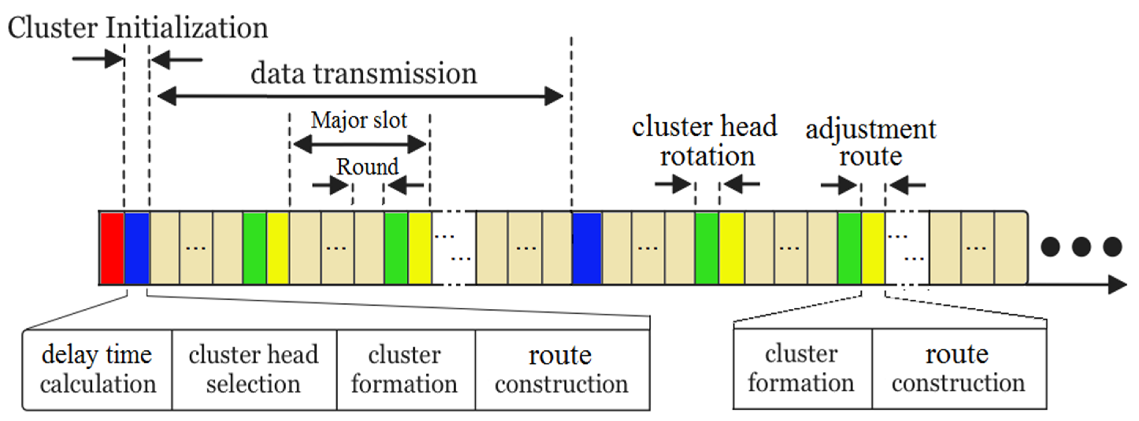
Proof of Lemma 1.

In this protocol it is assumed that N is the number of nodes, r is the number of rounds in a major slot, M refers to the number of major slots in data transmission, and R is the number of rounds in a data transmission, which is equal to r × M. □

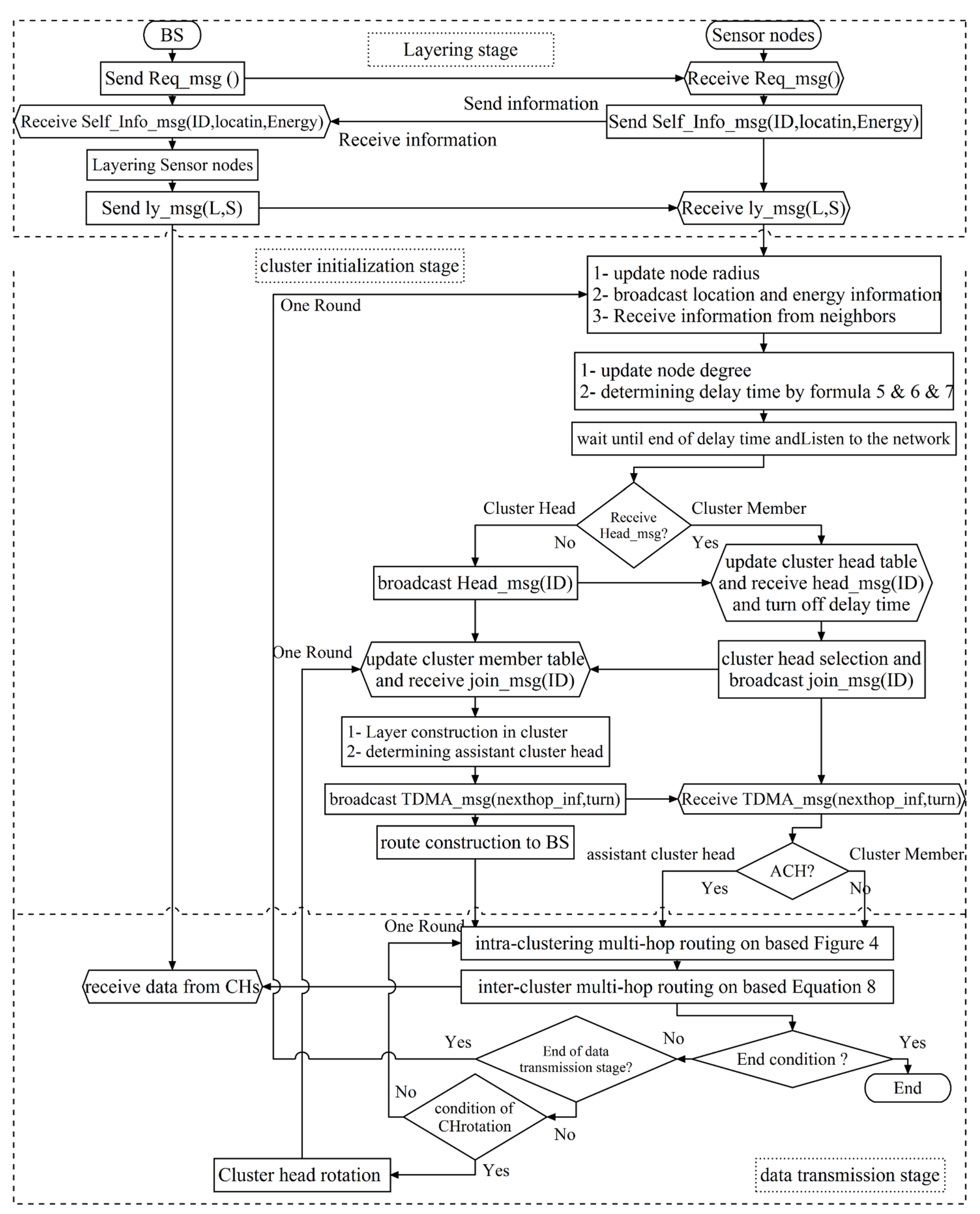
During the layering stage BS broadcasts a message in the network. Subsequently, node N transmits self_info_msg to BS and BS broadcasts cmd_msg message in the network. Therefore, N + 2 messages are required for this stage. In the cluster initialization stage, node N broadcasts node_msg including information on node energy and location. Then, the K times head_msg is broadcasted by CHs and N − k join_msg messages are transmitted to the CHs by CM. Consequently, K messages of TDMA_msg are broadcasted by CHs. Moreover, 2K control messages are required for constructing the data transmission path to the BS. Therefore, N + K + (N − K) + K + 2K = 2N + 3K messages are required for clustering. In total, 3N + 3K + 2 messages are required during the above-mentioned stages. Therefore, in the worst case scenario, the control message complexity is of type O(N).

In hybrid performance, it is not necessary to perform clustering in each round and data transmission is performed with M major slot, which consists of r rounds. For CH rotation and route adjustment, maximum (N − K) + K and K + 2K messages are required, respectively. Therefore, in the data transmission stage, [(M − 1) × ((N − k) + k + k + 2k)] = (M − 1) × (N + 3k) messages are needed.

Lemma 2.

If there is a node within the competition radius area of another node, then the presence of two CHs is impossible.

Proof of Lemma 2.

According to Equation (7), each node has a unique delay time. If a node has a lesser delay time, it transmits head_msg with Rc(i) radius and all other nodes with this radius change their own position to CM. Therefore, if there are two nodes located within competition radius, it is not possible to have more than two CHs. □

Lemma 3.

After performing HCD, whole network space is covered by CHs; in other words, a node (either CH or CM) will be in the same cluster.

Proof of Lemma 3.

If a node such as A is neither a CH nor a CM after performing HCD, node A will have two positions before executing the algorithm: (1) it does not have any neighbors and (2) has a neighbor. In the first case, according to the algorithm, node A announces to be the cluster head at the end of the delay time. In the second position, given that node A is a CH nor a CM, none of the neighbor nodes broadcast the CH message. If one of them was CH, then A will be a CM. However, if A and some of its neighbors are not CH and they do not join to a cluster, then one of them will be converted to the CH after the end of delay time. Subsequently, a message is broadcasted and neighbor nodes receiving the message will change their positions to the CMs. Therefore, node A will be either a CH or will join another CH before the end of the algorithm. Hence, it can be said that the network is completely covered by CHs. □

Lemma 4.

The HCD guarantees the load balancing of CHs in intracluster and intercluster multihop routing.

Proof of Lemma 4.

According to the Equation (4), it can be demonstrated that the node radius depends on its distance to the BS and its remaining energy. Therefore, CHs having more distance to BS and higher remaining energy make larger clusters and they have more CMs. Hence, it consumes more energy to receive and collect data from CMs. Moreover, ACH nodes are applied to maximize the stability and balanced energy consumption of CMs during data transmission to the CH and also to balance CH energy consumption for receiving the data. On the other hand, CHs close to the BS with less energy have a smaller radius and less CMs. Therefore, they save more energy for receiving and collecting data from the CMs, and they guarantee the load balancing of the HCD protocol. □

5. Simulation Results

The main purpose of this research was to reduce energy consumption and increase the network life time. In order to achieve this purpose, simulations were performed in MATLAB programming environment. Furthermore, to evaluate network stability, efficiency, and throughput of the proposed algorithm, this algorithm was compared to ECDC (2013) [24], HUCL (2015) [15], and EADUC-II (2016) [25] algorithms.

5.1. Simulation Scenarios

We also performed simulations for two different states shown in

Table 2. Scenarios.

Network	BS	Number of Node	Network Space
scenarios #1	(100,250)	100	200 × 200
scenarios #2	(100,100)	100	200 × 200

. In the first scenario, there are 100 nodes in 200 × 200 spaces and the BS is located outside the network space and located at 100 × 250. In the second scenario, the location of the BS has changed to the network center and 100 × 100 location.

In the proposed algorithm the count of alive nodes, the average of network energy and network stability, first node death (FND), half node death (HND), death of 10% and 20% of nodes (PND), and last node death (LND) during the whole simulation time were evaluated. The simulation was performed in 50 periods.

Definitions of some important concepts:

• Network lifetime: the time interval from the start of network operations to LND.
• Network stability: the time interval from the start of the network operations to FND.
• Throughput or efficiency: the number of data packets sent by a network to the BS. Efficiency improvement has a direct co-relation with increased network stability and the network lifetime.
• Load balancing: traffic load distribution. Its advantage is that when the load is well-distributed throughout the nodes, it results in balanced energy consumption. It also prevents the sudden death of the nodes caused by overusing them and increases the network stability.

5.2. Simulation Parameters

Simulation parameters are displayed in

Table 3. Parameters used in the simulation.

Parameters	The Amount
Eelec	50 nJ/bit
Efs	10 pJ/bit/m2
Emp	0.0013 pJ/bit/m4
EDA	5 nJ/bit/message
Data packet size	1000 byte
Packet header size	25 byte
Control message size	50 byte
RLmax	10–160 m
α, β	0.333
Initial energy	0.5–1.5 j
Number of rounds in a Major slot	6
Number of Major slots in the data transmission stage	7

. The optimum values of some of the parameters (for example RL_max) were determined from various simulation results.

We performed simulations several times to determine the round numbers in a major slot (Figure 2) and major slot in data transmission stage (Figure 2). Simulation parameters, such as the nodes locations, are considered to be the same for all the nodes so that the results are reliable and solid. This simulation plays a crucial role in the proposed protocol. In this protocol, by decreasing the number of rounds, we can more accurately simulate a dynamic method which results in increased overhead and energy consumption and declined the network life span. In contrast, by increasing the number of rounds the proposed protocol gets closer to the static methods and, therefore, leads to a decrease is overhead and loss of energy in CH and, subsequently, the stability and throughput of the network reduced. Since the main aim of the proposed protocol was to increase the maximum lifetime of the network by eliminating maximum control messages and reducing overhead which leads to the reduced energy consumption of networks nodes. The number of rounds in a major slot and the number of major slots in data transmission should be optimized. In order to determine the abovementioned optimized numbers, the simulation was performed several times. Considering the structure of the proposed method, we preferred to set the amount of the mentioned parameter to the highest value of FND. According to Figure 5 and Figure 6 we considered the count of rounds as 6 and the count of the major slot as 7. The optimum FND average was obtained in different simulations. According to the simulation results, it can be seen that each data transmission stage consists of 7 portions of the major slot including 6 rounds, one CH rotation, and one adjustment route. Overall, during the data transmission stage, data was transmitted in 42 rounds and we aimed to remove the majority of the network overhead.

For results and considered parameters refer to Figure 2. Figure 2 demonstrates the protocol performance considering the number of rounds and major slots. According to the results of Figure 5, we set the number of rounds and a major slot in Figure 2.

One of the most important parameters in clustering is to determine the radius. The radius of the nodes in each layer of the proposed protocol is intentionally considered as different sizes. Thus, the value of λ in Equation (4) in the first layer is equal to 1, in the second and third layers is 1.25, and in the fourth layer is 1.75. Thus, the clusters which are closer to the BS are smaller and the CH can have more energy for relaying and routing other CH packets to the BS. To determine the RL_max parameter in the Equation (4) we carried out various simulation runs with different RL_max values to obtain the optimum value for RL_max parameter. Two of the important factors in IoT-based wireless nodes are the number of CH and the size of clusters, which are dependent on the radius of the nodes. The simulation results for different scenarios are shown in Figure 7.

The radius of each node must be so that the number of cluster nodes in the network is reasonable. In the paper, the number of optimal CH was considered equal to 5% of the total number of nodes in the network. In our proposed protocol, we assumed that the value of RL_max parameter is equal to 100 m which makes the number of CH approximately equal to 5 based on [3].

Figure 8 and Figure 9 demonstrate the routing and clustering graph formed in one of the simulations for scenarios 1 and 2. Green nodes display CM nodes, turquoise color indicates ACH nodes, and CHs are indicated in blue color. According to these figures, clusters close to BS are smaller and as a result, they have more energy for distant CH data relay. In addition, ACH nodes cooperate with CH in data transmission. If the network area is larger, and the distance of nodes are farther, then the role of these nodes will be more effective.

5.3. Network Stability and Network Lifetime

In order to increase efficiency and throughput, we must transmit more data to the BS and, in this case, it is necessary to prevent node death. Therefore, efficiency and throughput can be improved by increasing network stability. In

Table 4. Simulation results of stability period and lifetime for scenario 1.

Protocol	FND (100 Nodes)		10% PND (90 Nodes)		20% PND (80 Nodes)		HND (50 Nodes)		LND (0 Nodes)
	Time	Packets	Time	Packets	Time	Packets	Time	Packets	Time	Packets
ECDC	251.6	25156	465.7	45795	541.6	52307	648.8	59245	1133.8	65685
HUCL	273.7	27367	524.7	51201	638.4	60591	737.9	66555	866	68843
EADUC-II	394.2	39422	608.8	60138	662.1	64636	691.3	66365	719.4	66685
HCD	702.2	70205	881.9	86164	918.3	88646	964	90641	1047.3	91263

and

Table 5. Simulation results of stability period and lifetime for scenario 2.

Protocol	FND (100 Nodes)		10% PND (90 Nodes)		20% PND (80 Nodes)		HND (50 Nodes)		LND (0 Nodes)
	Time	Packets	Time	Packets	Time	Packets	Time	Packets	Time	Packets
ECDC	345.2	34515	569.1	56204	644.9	62693	743.5	6900.7	1283.6	7620.3
HUCL	205.2	20518	489.8	47679	617.4	58584	736.8	66323	856.9	68948
EADUC-II	358.1	35808	590.5	58125	667.9	65680	712.4	67864	742.5	68265
HCD	863.5	86348	966.7	96087	983.4	97222	1013.6	98538	1088.3	99168

, the performance of the stability period and the network lifetime involving FND, 10% PND, 20% PND, HND, and LND of the protocols was determined for the first and second scenarios. In both scenarios, the proposed protocol had better performance compared to ECDC, HUCL, and EADUC-II algorithms. Our proposed method had significantly improved performance with very high stability in two different spaces. HCD gets help from the information of neighbor nodes for clustering and uses intercluster and intracluster as well as multihop transmission appropriately. In Table 4 and Table 5, the obtained results indicate that the proposed protocol could improve some parameters and be able to transmit more packets in the event of these parameters occurrence. It was emphasized that these nodes that do not have suitable energy status should not become a CH. Since CH node consumes more energy emphasizing this idea resulted in dividing energy consumption equally between the nodes during simulation time. The presented protocol helped reducing energy consumption in the network by deleting unusual control messages and reducing overhead; therefore, it resulted in a prolonged network lifetime.

Table 6. HCD protocol improvement in comparison with other protocols in simulation scenarios.

The Network	Parameters	HCD V ECDC	HCD V HUCL	HCD V EADUC-II
Scenarios 1	FND	179.30%	156.50%	78.10%
	10%PND	89.30%	68%	44.80%
	20%PND	69.50%	43.80%	38.60%
	HND	48.50%	30.60%	39.40%
	LND	% −7.6	20.90%	45.50%
Scenarios 2	FND	150.10%	320.80%	141.10%
	10%PND	69.80%	97.30%	63.70%
	20%PND	52.40%	59.20%	47.20%
	HND	36.30%	37.50%	42.20%
	LND	% −15.2	27%	46.50%

shows the performance of the proposed protocol in comparison to the other three protocols. In order to evaluate it better, we showed the improvement percentage of above-mentioned criteria in Table 6. The measurement showed that the presented protocol increased network stability considerably. The ECDC protocol acts as distributed and dynamic, but the protocols of HUCL, EADUC-II, and the proposed protocol act as hybrid and distributed. When HCD was compared to HUCL, it increased the network stability to 156.5% and 320.8% in the first and second scenarios, respectively. We compared the proposed protocol with EADUC-II and noticed that this protocol had increased the network stability to 78.1% and 141.1% in the first and second scenarios, respectively.

5.4. Number of Nodes Alive

In

Table 7. The average number of live nodes.

Protocol	Scenario 1	Scenario 2
ECDC	20.9	24.4
HUCL	22.6	22.8
EADUC-II	21.4	21.9
HCD	30.7	32.7

, the average number of live nodes is displayed. As it can be concluded from the Table 7, the average number of live nodes was more than 30% of all node counts which confirmed the maintained network stability as it was proposed by our algorithm. Figure 10 and Figure 11 demonstrate the number of live nodes during simulation. The results showed that HCD had better performance compared to other protocols and increased the number of live nodes during simulation. It was due to the balance between the energy consumption of different nodes as it was proposed by the presented protocol and therefore, could prevent node death.

5.5. The Average of the Energy of Alive Nodes

As it was assumed, the network is formed by heterogeneous nodes which have an energy between 0.5 to 1.5 j. Figure 12 illustrate the energy consumption of each node in the proposed algorithm and in scenario 1. Figure 12 and Figure 13 compare the amount of energy in each node in HCD for scenarios 1 and 2, at the beginning of the network and during the rounds 250, 500, and 750. The proposed protocol has excellent load balancing. At first, due to the assumption of heterogeneous nodes, an energy difference between the nodes is observed. However, gradually in a period of 250, and particularly 500, during the performance of our proposed protocol, it can be seen that the energy difference between nodes is reduced. This indicates that in the proposed protocol we have high load balancing. The proposed protocol is able to distribute the energy consumption between all nodes and pave the way for increasing the load balancing by selecting the proper CH. In addition, by determining the suitable CH, the presented protocol divided the energy consumption among nodes and it helped reducing energy consumption by multihop transmission. In this type of transmission distance is short, and hence, less energy is required for transmission. Accordingly, the presented protocol prevented the immediate reduction of energy in nodes by selecting appropriate CH and avoiding direct transmission to distant nodes. Consequently, the close and distant nodes consumed energy in a balanced way, the stability was increased and the throughput was improved.

One of the important reasons in the proposed protocol which contributed to the increased network lifetime is that it omitted the maximum control messages in the network. Figure 14 and Figure 15 show the energy consumption for control messages in the proposed protocol and other protocols. The proposed protocol decrease energy consumption in terms of control messages to 300% in comparison to EDCD and EADUC-II and 100% in comparison to HUCL.

Given that in our proposed protocol there were 6 rounds of data transmission per each major slot without the overhead control message, and since the protocol had 42 rounds of data transmission to the BS per each transmission stage, this protocol was able to optimize the energy consumption by reducing the overhead. This led to an increase in average energy of nodes. Figure 16 and Figure 17 show the average energy of alive nodes during the simulation.

According to the results, it can be concluded that in the proposed method by reducing the network overhead, the energy consumption has been reduced.

5.6. Throughput

Figure 18 and Figure 19 demonstrate packet production in relation to the round indicating an increased efficiency of the proposed protocols. This method was able to produce and transmit more packets during the simulation, increase the throughput due to the balanced energy consumption, increased stability and improved number of available nodes. The proposed protocol increases throughout to 40%, 33%, and 37% in the first scenario and 30%, 43%, and 45% in the second scenarios in comparison to ECDC, HUCL, and EADUC-II, respectively.

5.7. Simulation in Other Scenarios and Parameters

Based on the reliability of our proposed protocol in this section, we have compared this protocol with simulation scenarios of EADUC-II [25]. Therefore, the simulation parameters reported in [25] were considered. According to their first scenario, 100 nodes were distributed uniformly within an area of 200 ✕ 200 m² and the location of the BS was set at 250 ✕ 100. The size of the packets and control massage was 500 byte and 25 bytes, respectively. The results, as shown in Figure 20, indicated an improvement in the average number of alive nodes in comparison with the previous protocols.

Our simulation results with the parameters of the article [25], also confirm the simulation of the EADUC-II and the results showed that the proposed protocol had better performance compared to other protocols.

6. Conclusions

In recent years, the development of technology, IoT has been used over sensor networks in various fields. Wireless nodes have some limitation in case of energy sources since energy consumption is highly related to sending and receiving waves. Optimization of energy consumption in routing protocols is one of the main methods of increase the network lifetime. In this paper, we proposed a new and efficient clustering protocol based on density as a hybrid of static and dynamic as well as multi-hop routing for IoT based on wireless nodes. We considered a distributed clustering method and performed routing between CH and BS on the basis of multi-hop routing. The proposed method significantly reduced the network overhead and energy consumption by deleting unusual control messages. The results showed that HCD can effectively improve network stability and lifetime. Compared to EDCD [24], HUCL [15], and EADUC-II [25], the network stability increased to 179%, 156%, and 78% and to 150%, 320%, and 141% in the first and second scenarios, respectively. In addition, HCD increased throughput to 40%, 33%, and 37% in the first scenario and 30%, 43%, and 45% in the second scenarios in comparison to EDCD, HUCL, and EADUC-II. Furthermore, it is able to balance energy consumption in the network and improve efficiency and throughput.

References

1. Machado, K.; Rosário, D.; Cerqueira, E.; Loureiro, A.; Neto, A.; de Souza, J. A Routing Protocol Based on Energy and Link Quality for Internet of Things Applications. Sensors 2013, 13, 1942–1964. [Google Scholar] [CrossRef] [PubMed] [Green Version]
2. Abdul-Qawy, A.S.H.; Srinivasulu, T. SEES: A scalable and energy-efficient scheme for green IoT-based heterogeneous wireless nodes. J. Ambient Intell. Hum. Comput. 2018. [Google Scholar] [CrossRef]
3. Heinzelman, W.B.; Chandrakasan, A.P.; Balakrishnan, H. An application-specific protocol architecture for wireless microsensor networks. IEEE Trans. Wirel. Commun. 2002, 1, 660–670. [Google Scholar] [CrossRef] [Green Version]
4. Zhang, W.; Wei, X.; Han, G.; Tan, X. An Energy-Efficient Ring Cross-Layer Optimization Algorithm for Wireless Sensor Networks. IEEE Access. 2018, 6, 16588–16598. [Google Scholar] [CrossRef]
5. Xiao, F.; Liu, W.; Li, Z.; Chen, L.; Wang, R. Noise-Tolerant Wireless Sensor Networks Localization via Multinorms Regularized Matrix Completion. IEEE Trans. Veh. Technol. 2018, 67, 2409–2419. [Google Scholar] [CrossRef]
6. Qiao, J.; Zhang, X. Polar Coordinate-Based Energy-Efficient-Chain Routing in Wireless Sensor Networks Using Random Projection. IEEE Access 2018, 6, 21275–21286. [Google Scholar] [CrossRef]
7. Bozorgi, S.M.; Rostami, A.S.; Hosseinabadi, A.A.R.; Balas, V.E. A new clustering protocol for energy harvesting-wireless sensor networks. Comput. Electr. Eng. 2017, 64, 233–247. [Google Scholar] [CrossRef]
8. León, O.; Hernández-Serrano, J.; Soriano, M. Securing cognitive radio networks. Int. J. Commun. Syst. 2010, 23, 633–652. [Google Scholar] [CrossRef]
9. Wang, J.; Li, B.; Xia, F.; Kim, C.S.; Kim, J.U. An Energy Efficient Distance-Aware Routing Algorithm with Multiple Mobile Sinks for Wireless Sensor Networks. Sensors 2014, 14, 15163–15181. [Google Scholar] [CrossRef]
10. Yan, J.; Zhou, M.; Ding, Z. Recent Advances in Energy-Efficient Routing Protocols for Wireless Sensor Networks: A Review. IEEE Access 2016, 4, 5673–5686. [Google Scholar] [CrossRef]
11. Wang, J.; Cao, J.; Li, B.; Lee, S.; Sherratt, R.S. Bio-inspired ant colony optimization based clustering algorithm with mobile sinks for applications in consumer home automation networks. IEEE Trans. Consum. Electron. 2015, 61, 438–444. [Google Scholar] [CrossRef]
12. Kumar, A.; Kumar, V.; Chand, N. Energy Efficient Clustering and Cluster Head Rotation Scheme for Wireless Sensor Networks. Int. J. Adv. Comput. Sci. Appl. 2011, 3, 129–136. [Google Scholar] [CrossRef]
13. Chaurasiya, S.K.; Pal, T.; Bit, S.D. An Enhanced Energy-Efficient Protocol with Static Clustering for WSN. In Proceedings of the International Conference on Information Networking 2011 (ICOIN2011), Barcelona, Spain, 26–28 January 2011; pp. 58–63. [Google Scholar]
14. Zanjireh, M.M.; Larijani, H. A Survey on Centralised and Distributed Clustering Routing Algorithms for WSNs. In Proceedings of the 2015 IEEE 81st Vehicular Technology Conference (VTC Spring), Glasgow, UK, 11–14 May 2015; pp. 1–6. [Google Scholar]
15. Malathi, L.; Gnanamurthy, R.K.; Chandrasekaran, K. Energy efficient data collection through hybrid unequal clustering for wireless sensor networks. Comput. Electr. Eng. 2015, 48, 358–370. [Google Scholar] [CrossRef]
16. Rostami, A.S.; Badkoobe, M.; Mohanna, F.; Hosseinabadi, A.; Hosseinabadi, A.R.; Sangaiah, A.K. Survey on Clustering in Heterogeneous and Homogeneous Wireless Sensor Networks. J. Supercomput. 2018, 74, 277–323. [Google Scholar] [CrossRef]
17. Bozorgi, S.M.; Amiri, M.G.; Rostami, A.S.; Mohanna, F. A novel dynamic multi-hop clustering protocol based on renewable energy for energy harvesting wireless sensor networks. In Proceedings of the 2015 2nd international conference on knowledge-based engineering and innovation (KBEI), Tehran, Iran, 5–6 November 2015; pp. 619–624. [Google Scholar]
18. Rostami, A.S.; Bernety, H.M.; Hosseinabadi, A.R. A Novel and Optimized Algorithm to Select Monitoring Sensors by GSA. In Proceedings of the IEEE International Conference on Control, Instrumentation and Automation (ICCIA), Shiraz, Iran, 27–28 December 2011; pp. 829–834. [Google Scholar]
19. Ruiz, M.T.; Lytras, M.D.; Mathkour, H. Innovative services and applications of wireless sensor networks: Research challenges and opportunities. Int. J. Distrib. Sens. Netw. 2018, 14, 1–4. [Google Scholar]
20. Younis, O.; Fahmy, S. HEED: A hybrid, energy-efficient, distributed clustering approach for ad hoc sensor networks. IEEE Trans. Mob. Comput. 2004, 3, 366–379. [Google Scholar] [CrossRef]
21. Lee, K.; Lee, J.; Lee, H.; Shin, Y. A Density and Distance based Cluster Head Selection algorithm in Sensor Networks. In Proceedings of the 2010 The 12th International Conference on Advanced Communication Technology (ICACT), Phoenix Park, Korea, 7–10 February 2010; pp. 162–165. [Google Scholar]
22. Taheri, H.; Neamatollahi, P.; Younis, O.M.; Naghibzadeh, S.; Yaghmaee, M.H. An energy-aware distributed clustering protocol in wireless sensor networks using fuzzy logic. Ad Hoc Netw. 2012, 10, 1469–1481. [Google Scholar] [CrossRef]
23. Ducrocq, T.; Mitton, N.; Hauspie, M. Energy-based clustering for wireless sensor network lifetime optimization. In Proceedings of the 2013 IEEE Wireless Communications and Networking Conference (WCNC), Shanghai, China, 7–10 April 2013; pp. 968–973. [Google Scholar]
24. Gu, X.; Yu, J.; Yu, D.; Wang, G.; Lv, Y. ECDC: An energy and coverage-aware distributed clustering protocol for wireless sensor networks. Comput. Electr. Eng. 2014, 40, 384–398. [Google Scholar] [CrossRef]
25. Gupta, V.; Pandey, R. An improved energy aware distributed unequal clustering protocol for heterogeneous wireless sensor networks. Eng. Sci. Technol. 2016, 19, 1050–1058. [Google Scholar] [CrossRef] [Green Version]
26. Sabor, N.; Abo-Zahhad, M.; Sasaki, S.; Ahmed, S.M. An Unequal Multi-hop Balanced Immune Clustering protocol for wireless sensor networks. Appl. Soft Comput. 2016, 43, 372–389. [Google Scholar] [CrossRef]
27. Meng, X.; Shi, X.; Wang, Z.; Wu, S.; Li, C. A grid-based reliable routing protocol for wireless sensor networks with randomly distributed clusters. Ad Hoc Netw. 2016, 51, 47–61. [Google Scholar]
28. Chen, D. An energy-efficient QoS routing for wireless sensor networks using self-stabilizing algorithm. Ad Hoc Netw. 2015, 37, 240–255. [Google Scholar] [CrossRef]
29. Chanak, P.; Banerjee, I.; Sherratt, R.S. Energy-Aware Distributed Routing Algorithm to Tolerate Network Failure in Wireless Sensor Networks. Ad Hoc Netw. 2016, 56, 158–172. [Google Scholar]
30. Naeem, M.K.; Patwary, M.; Abdel-Maguid, M. Universal and Dynamic Clustering Scheme for Energy Constrained Cooperative Wireless Sensor Networks. IEEE Access 2017, 5, 12318–12337. [Google Scholar] [CrossRef]
31. Cengiz, K.; Dag, T. Energy Aware Multi-Hop Routing Protocol for WSNs. IEEE Access 2018, 6, 2622–2633. [Google Scholar] [CrossRef]
Figure 1. Components of the sensor node.
Sustainability 11 00746 g001
Figure 2. Hybrid unequal multihop clustering based on density (HCD) operation.
Sustainability 11 00746 g002
Figure 3. Flowchart of the HCD protocol.
Sustainability 11 00746 g003
Figure 4. Routing flowchart of intraclustering in HCD.
Sustainability 11 00746 g004
Figure 5. Network lifetime under different rounds in different major slots at data transmission stage for scenario #1 with Rlmax = 100 and initial energy = 1 J.
Sustainability 11 00746 g005
Figure 6. Network lifetime under different rounds in different major slots at data transmission stage for scenario #2 with Rlmax = 100 and initial energy = 1 J.
Sustainability 11 00746 g006
Figure 7. CH generated in two scenarios.
Sustainability 11 00746 g007
Figure 8. Routing and clustering graph for scenario 1.
Sustainability 11 00746 g008
Figure 9. Routing and clustering graph for scenario 2.
Sustainability 11 00746 g009
Figure 10. The average of the number of alive nodes for scenario 1.
Sustainability 11 00746 g010
Figure 11. The average of the number of alive nodes for scenario 2.
Sustainability 11 00746 g011
Figure 12. Energy consumption of HCD for scenario 1.
Sustainability 11 00746 g012
Figure 13. Energy consumption of HCD for scenario 2.
Sustainability 11 00746 g013
Figure 14. Total energy consumption for control message in scenario 1.
Sustainability 11 00746 g014
Figure 15. Total energy consumption for control message in scenario 2.
Sustainability 11 00746 g015
Figure 16. The average energy of alive nodes for scenario 1.
Sustainability 11 00746 g016
Figure 17. The average of the energy of alive nodes for scenario 2.
Sustainability 11 00746 g017
Figure 18. Throughput for scenario 1.
Sustainability 11 00746 g018
Figure 19. Throughput for scenario 2.
Sustainability 11 00746 g019
Figure 20. The average of the number of alive nodes for our Simulation.
Sustainability 11 00746 g020