Quantitative Multi-Hazard Risk Assessment of Crop Loss in the Yangtze River Delta Region of China

Abstract

Due to their complexity, hazard interactions are often neglected in current studies of multi-hazard risk assessment. As a result, the assessment results are qualitative or semi-quantitative and are difficult to use in regional risk management. In this paper, the crop loss risk due to heavy rain and strong wind in the Yangtze River Delta (YRD) region of China was quantitatively assessed, based on the joint return periods of these hazards and a vulnerability surface. The joint return period is obtained with a copula function based on the marginal distribution of each hazard. The vulnerability is fitted by considering the joint hazard intensity, the sown area of crops, elevation, and GDP per capita. The results show that counties with a high value of joint hazard probability are clustered in the southeast coastal area and that the value gradually decreases from south to north and from east to west. The multi-hazard risk has a similar pattern, with a large value in the southeast coastal area and a low value in the northwest. The proposed method can be used for quantitative assessment of multi-hazard risk, and the results can be used for regional disaster risk management and planning.

1. Introduction

Along with global climate change and rapid economic development, our societies are facing great threats from natural disasters. Frequent and intense natural disasters may threaten to reverse much of the developmental progress that has been made in recent decades. Strengthening the capacity for adaptation to climate change, extreme weather, drought, flooding, and other disasters is one of the sub-goals of the Sustainable Development Goals 2030 [1]. Risk assessment is one effective and important step in enhancing a region’s coping capacity to natural disasters. As most areas on Earth are likely to be influenced by more than one hazard, a single natural disaster risk cannot represent the total risk level of each region [2]. For better disaster risk management, it is important to assess the regional risks of multiple hazards.

Recently, many models or indexes have been developed and applied to assess the risks of multiple hazards. Typical examples are the Disaster Risk Index [3], the Hotspots Index [4], the World Risk Index [5], the ESPON method [6], the INFORM [7], the Total Risk Index [8], and the Multi-Hazard Index [8,9,10]. However, the calculated risks based on the above models, methods, or indexes are all qualitative or semi-quantitative. The Global Risk Model, which is a quantitative multi-hazard risk assessment model led by the United Nations International Strategy for Disaster Reduction (UNISDR) to calculate the annual average loss (AAL) of multiple hazards by adding up the AAL of each individual hazard, is used as the basis for the Global Assessment Report (GAR) 2013 [11], the GAR 2015 [12], and the GAR ATLAS of 2017 [13]. The information diffusion method is also used for quantitatively calculating multi-hazard risks, e.g., the risks of typhoon and flood in the Yangtze River Delta (YRD) region of China [14] and multiple climatic hazards of China [15]. However, in both the Global Risk Model and the diffusion method, the interactions between the different hazards are not considered. If the hazards are dependent, then the expected loss of multiple hazards cannot be directly summed by the loss of individual hazards [2,16], e.g., for wind and storm surge [17], and for earthquakes, rainfall-triggered landslide, and volcanos [18]. A copula function has been tested and has proved to be useful in quantitatively assessing the joint probability distributions of multiple hazards, although the process is complicated [19,20,21].

In this paper, the multi-hazard risks are quantitatively assessed based on a copula function and multi-dimensional vulnerability. The proposed method is demonstrated with the crop loss risk to heavy rain and strong winds in the YRD region of China. In the risk assessment method, the joint distributions of heavy rain and strong wind were calculated by using the copula theory, and the vulnerability surface was fitted by applying trend surface analysis and multiple regression estimation. Based on the joint distributions of multiple hazards and the vulnerability surface, the expected crop loss risks were quantitatively calculated.

2. Study Area and Data

2.1. Study Area

The study area is the Yangtze River Delta (YRD) region, which is located in the east coast of China (Figure 1) and includes 16 municipalities: Nanjing, Suzhou, Wuxi, Yangzhou, Changzhou, Nantong, Taizhou (J), and Zhenjiang of Jiangsu Province; Hangzhou, Jiaxing, Huzhou, Zhoushan, Shaoxing, Ningbo, and Taizhou (Z) of Zhejiang Province; and Shanghai.

The YRD region is a highly developed metropolitan area with a total population of 1.11 × 10⁸ people and a GDP of 9.62 × 10¹² yuan in 2016. The region is also an important agricultural region; it had a crop planting area of 3.18 × 10⁷ ha and the crop production of 5.86 × 10⁹ kg in 2016. The geographic features make the region vulnerable to typhoon and flood. According to historical data, the region was affected by five typhoons and four floods, causing damage to a crop planting area of approximately 7.68 × 10⁵ ha yearly from 1981 to 2010. More than 60% of the total crop loss during this period is from these two hazards [14]. Therefore, it is necessary to study the multi-hazard risks of crop loss for disaster risk management in this region. This study tries to analyze the joint risk of crop loss due to concurrent heavy rain and strong wind, which are identified as the main two factors affecting agricultural production in the region.

2.2. Data and Preprocessing

There are four types of data used in this study: meteorological data, socioeconomic data, crop loss data, and geographic data (including digital elevation model (DEM) and an administrative map). The hazard data of heavy rain and wind speed from 1971 to 2011, which are derived from the national meteorological data service center, include data from the 34 national standard monitoring stations of the study area and vicinity. Daily meteorological data were interpolated to the center points of each county by using the nearest neighboring point. Only a certain intensity of rainfall and wind speed was regarded as a hazard factor that can cause damage to crops. The thresholds for daily precipitation and the annual maximum wind speeds were set at 25 mm and 8 m/s, respectively. Therefore, the multi-hazard joint probability scenario in this study involved daily rainfall greater than or equal to 25 mm and a daily maximum wind speed greater than or equal to 8 m/s. In this study, the crop loss was represented by the area of crops affected by the natural disasters. The data from 1971 to 2011 were provided by the Ministry of Civil Affairs. The crop loss rate, which was calculated as the area affected by natural disasters divided by the crop planting area, was used in this study. The crop loss, whose time and venue match with the periods and areas affected by heavy rain and wind hazards, were recognized as the loss jointly caused by these two hazards. In total, 162 samples were obtained. Each sample, which includes the information of crop loss rate, precipitation, and wind speeds, was used to fit the vulnerability surface. The socioeconomic data, including the total population, GDP, GDP per capita, land area, crop planting area, total rural machinery power and machinery power per square kilometer, etc. for each county were taken from the statistical yearbooks of Shanghai, Jiangsu, and Zhejiang from 1990 to 2011. The social and economic indicators were used to adjust the vulnerability surface. The DEM data and administrative map were from the Ministry of Natural Resources. The DEM data was used to calculate the average elevation of each county.

3. Method

3.1. Fitting the Joint Distribution Based on a Copula

The joint probability distribution of rainfall and wind cannot be directly multiplied by the two marginal distributions because they are two independent variables [19]. In this paper, a copula function was used to construct their joint distribution. Given the two random variables X (representing rainfall) and Y (representing the maximum wind speed) for each county, the marginal distributions of F_X(x) and F_Y(y) can be fitted. The root mean square errors of these fitted functions were compared to obtain the best fitting parameters, and the edge distribution results were tested via the Chi-square test. Then, the two-dimensional distribution F_X,Y(x,y) could be calculated with a copula function based on Sklar’s theorem. Gumbel, Clayton, and Frank, which have only one parameter and can easily be calculated, are three common copulas. This study uses the maximum pseudolikelihood estimator to estimate the parameters for the copula functions.

After obtaining the fitting parameters of the marginal distribution and the joint distribution, the joint return period of rain and wind in this study could be obtained according to Equation (1).

$$T(x,y)=\frac{M_t}{P(X\ge x,Y\ge y)}=\frac{M_t}{1-F_X(x)-F_Y(y)+F_{X,Y}(x,y)}$$

(1)

where T(x, y) is the joint return period of rainfall (rainfall ≥ x) and wind (wind speed ≥ y) and F_X(x) and F_Y(y) are the cumulative distribution functions of rainfall (F_X(x) = P{X ≤ x}) and wind (F_Y(y) = P{Y ≤ y}), respectively. F_X,Y(x,y) is the joint probability distribution for rainfall and wind. Mt is the annual average number of joint events, which was calculated by dividing the total number of events by the number of years (41 years, 1971–2011 in this study).

3.2. Fitting the Vulnerability Surface

Vulnerability consists of the characteristics and circumstances of exposure that make something susceptible to the damaging effects of a hazard [21]. That is, both internal and extrinsic attributes determine vulnerability. The internal attribute depends on the biophysical characteristics of exposure. The extrinsic attribute of exposure, which is the vulnerability of the built environment, can be determined by various indicators. In this study, eight indicators (i.e., land area, crop planting area, average elevation, total population, GDP, GDP per capita, total rural machinery power, and machinery power per square kilometer) were selected to denote the extrinsic attribute of exposure.

Vulnerability, considering both the internal and extrinsic characteristics of this study, can be modeled according to Equation (2):

$$L=z(x,y)+EV$$

(2)

where L is the disaster loss; x and y are the precipitation and wind speed, respectively; and z(x, y) and EV reflect the internal and extrinsic characteristics of vulnerability, respectively. z(x,y) can be calculated according to Equations (3) and (4), and EV is determined by the eight indicators mentioned above and fitted according to Equation (5).

$$\mathrm{l}({\mathrm{x}}_{\mathrm{i}},{\mathrm{y}}_{\mathrm{i}})=\mathrm{z}({\mathrm{x}}_{\mathrm{i}},{\mathrm{y}}_{\mathrm{i}})+{\mathsf{\epsilon }}_{\mathrm{i}}\hspace{1em}(\mathrm{i}=1,2,\dots ,\mathrm{n})$$

(3)

$$\mathrm{z}({\mathrm{x}}_{\mathrm{i}},{\mathrm{y}}_{\mathrm{i}})={\mathrm{A}}_0+{\mathrm{A}}_1{\mathrm{x}}_{\mathrm{i}}+{\mathrm{A}}_2{\mathrm{y}}_{\mathrm{i}}+{\mathrm{A}}_3{\mathrm{x}}_{\mathrm{i}}{}^2+{\mathrm{A}}_4{\mathrm{x}}_{\mathrm{i}}{\mathrm{y}}_{\mathrm{i}}+{\mathrm{A}}_5{\mathrm{y}}_{\mathrm{i}}{}^2$$

(4)

$$EV=B_0+B_1{x}_1+B_2{x}_2+\dots +B_8{x}_8$$

(5)

where l(x_i,y_i) is the observed loss caused by precipitation and wind for sample i, z(x_i,y_i) is the fitted value, and ε_i is the residual. A₀, A₁…A₆ and B₀, B₁, …, B₈ are the coefficients that will be estimated using the least-squares method.

3.3. Calculating the Multi-Hazard Risk

The maximum crop loss rate at a return period (T0) can be expressed as follows.

$$L_0=max(L(x,y)),\hspace{1em}(x,y)\in \{(x,y) | T(x,y)=T_0\}$$

(6)

where T(x,y) is the joint return period calculated according to Equation (1) and L(x,y) is the vulnerability surface obtained according to Equation (2). Thus, the relationship between crop loss rate (L) and the return period (T) can be calculated. According to the loss–return period relationship, the relationship between the annual frequency (N) and loss can easily be calculated since N is the reciprocal of T. Thus, the loss-frequency curve, which is also a typical way to present the risk, can be obtained. The area between the curve and the two axes denotes the expected annual crop production loss. The larger the area is, the greater the expected annual loss rate.

4. Results

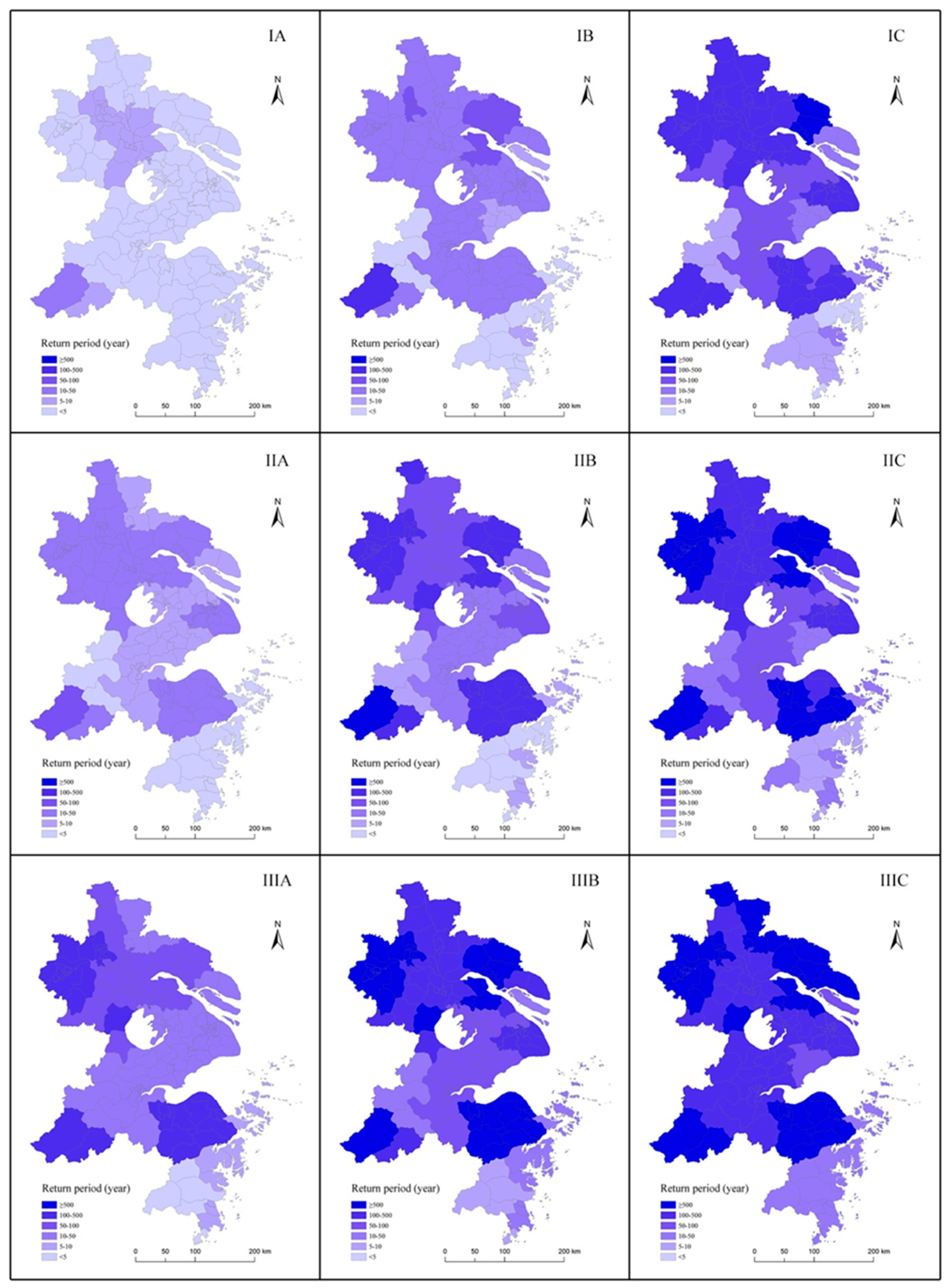
4.1. Joint Return Period for Rain and Wind

4.1.1. Parameter Fitting Result of the Copula Function

The Weber distribution, the generalized Pareto distribution, and extreme value distribution were all well applied to precipitation distribution fitting, and the Weibo distribution and the extreme value distribution were widely used for wind speed [13]. After comparison, the generalized extreme value distribution, which can be calculated using Equation (7), was found to be the best fitting for the marginal distribution of rainfall and wind speed in this study:

$$F(x;\mu ,\sigma ,\xi )=e^{-{[1+\xi (\frac{x-\mu }{\sigma })]}^{-1/\xi }}$$

(7)

where μ, σ, and ξ are the shape parameter, scale parameter, and position parameter of the generalized extreme value distribution, respectively.

In this study, these parameters were estimated by maximum likelihood estimation. The marginal distribution result of each county passed a Chi-square test with a confidence level of 95%. According to the above steps, the marginal and joint distributions of rain and strong wind for 140 counties in the YRD region were fitted. Taking Chongming, Jiangyin, Shaoxing, Lin’An, Fenghua, and Tongzhou as examples, the estimated parameters of the marginal and joint distributions are shown in

Table 1. Parameter estimation for the marginal and joint distributions of some counties in the YRD region.

Parameter		Chongming		Jiangyin		Shaoxing		Lin’an		Fenghua		Tongzhou
		X	Y	X	Y	X	Y	X	Y	X	Y	X	Y
$\mathsf{\mu }$		0.77	0.47	0.66	0.36	0.51	0.31	0.65	0.13	0.38	0.42	0.58	0.21
$\mathsf{\sigma }$		8.80	1.23	8.93	1.03	7.79	1.53	8.49	3.21	11.44	0.93	11.58	1.08
$\mathsf{\xi }$		32.76	9.34	33.67	9.23	32.62	9.86	32.70	11.94	37.13	9.07	36.34	9.35
Copula	Type	Gumbel		Gumbel		Frank		Frank		Clayton		Clayton
	θ	1.1496		1.0807		-0.3269		0.5267		0.3587		0.5330

. Evidently, Chongming and Jiangyin are a Gumbel copula, Shaoxing and Lin’an are a Frank copula, and Fenghua and Tongzhou are a Clayton copula.

4.1.2. Joint Hazard Analysis

Figure 2 shows the joint probability distribution in Chongming, Jiangyin, Shaoxing, Lin’An, Fenghua, and Tongzhou. The x-axis is precipitation, the y-axis is the wind speed, and the z-axis is the joint probability distribution of rainfall and wind speed that is less than or equal to the set value. The joint probability distribution increases with the increase in rainfall and wind speed. With a certain rainfall and wind speed, the joint probability distribution can easily be obtained from Figure 2. With a certain joint probability distribution (p), there exists group pairs of rainfall and wind speed, which are the intersecting curves of the joint probability distribution surface and the surface of z = p.

Figure 3 shows the joint return period of rainfall and strong wind in Chongming, Jiangyin, Shaoxing, Lin’an, Fenghua, and Tongzhou. Evidently, the joint return period increases with the increase in heavy rain and strong wind. Because of the relatively large range of the joint return period, the distribution images of these six counties clearly differ.

The intensity and probability/occurrence relationship shown in the joint probability/return period distribution effectively characterizes the joint hazard and can also be directly applied for the quantitative assessment of the multi-hazard risk.

4.1.3. Multi-Hazard Return Period

To further compare the multi-hazard characteristics in different counties, the joint return period for different types of rainfall and wind speed were calculated. Rainfall was divided into three types according to daily precipitation: type I (50–99.9 mm of daily rainfall), type II (100–249.9 mm), and type III (above 250 mm). Wind was also divided into three types according to the maximum wind speed: type A (10–17.1 m/s), type B (17.2–24.4 m/s), and type C (above 24.5 m/s). Based on Equation (6), the joint return periods of different types of rainfall and wind for the 140 counties can be obtained. The results are shown in Figure 4.

The darker the color is, the larger the joint return period and the smaller the probability of joint occurrence. Figure 4 shows that as the rainfall and wind speed increase, the return period shows an increasing trend. That is, the probability of occurrence decreases. The return period is more sensitive to a change in wind speed than to a change in rainfall.

Geographically, the counties in the northwest had a larger joint return period than those in the southeast, and the central counties had a larger joint return period than those on the coast. This finding means that the joint probability of heavy rainfall and wind for the southeast counties in the YRD region was greater than that of the northwest counties and that the joint probability of heavy rainfall and wind for the coastal counties is greater than that for the interior counties. The southeastern coastal areas, which are at a lower latitude, were frequently affected by tropical cyclones, which made the region have a higher probability of rainfall and wind.

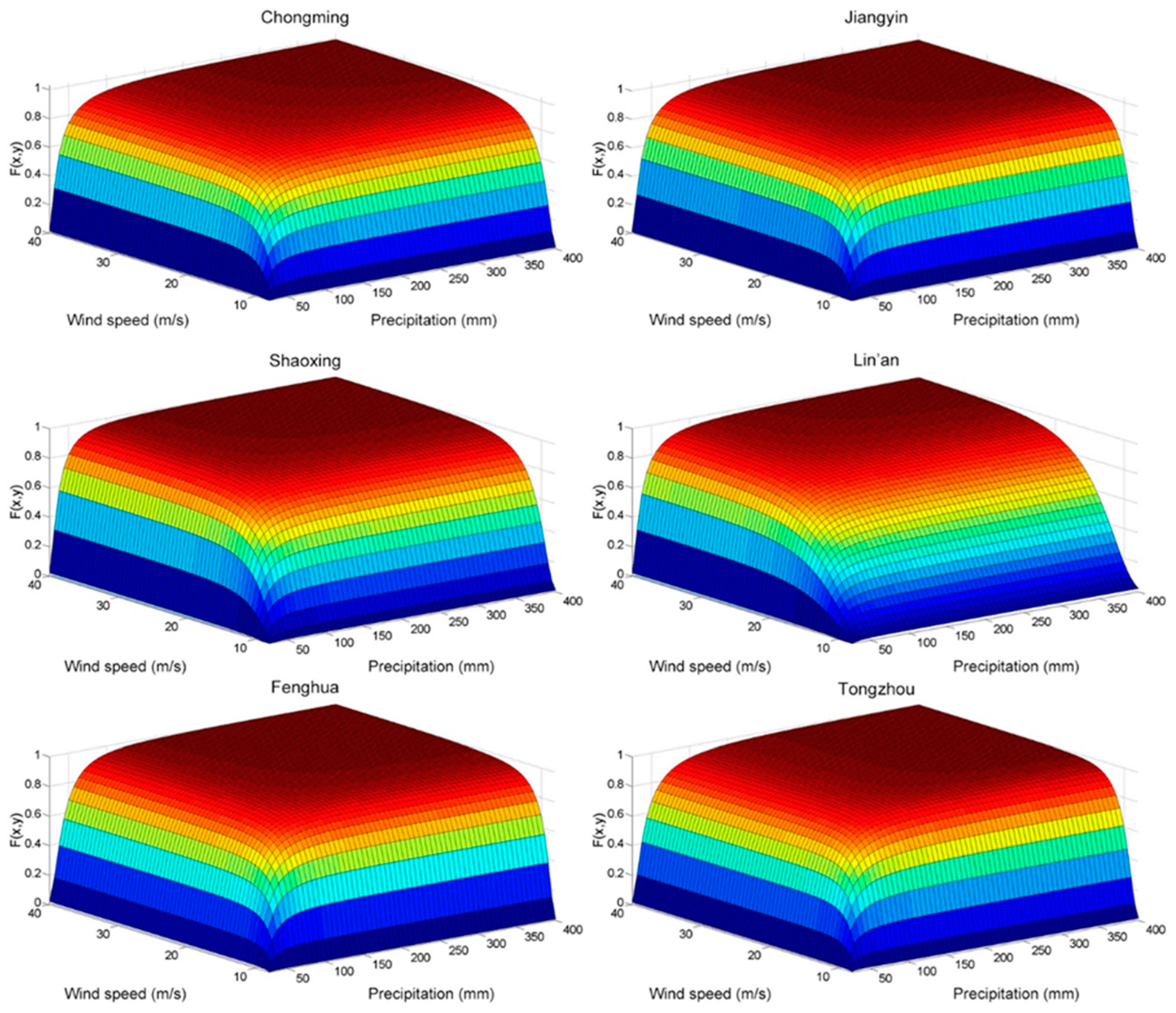
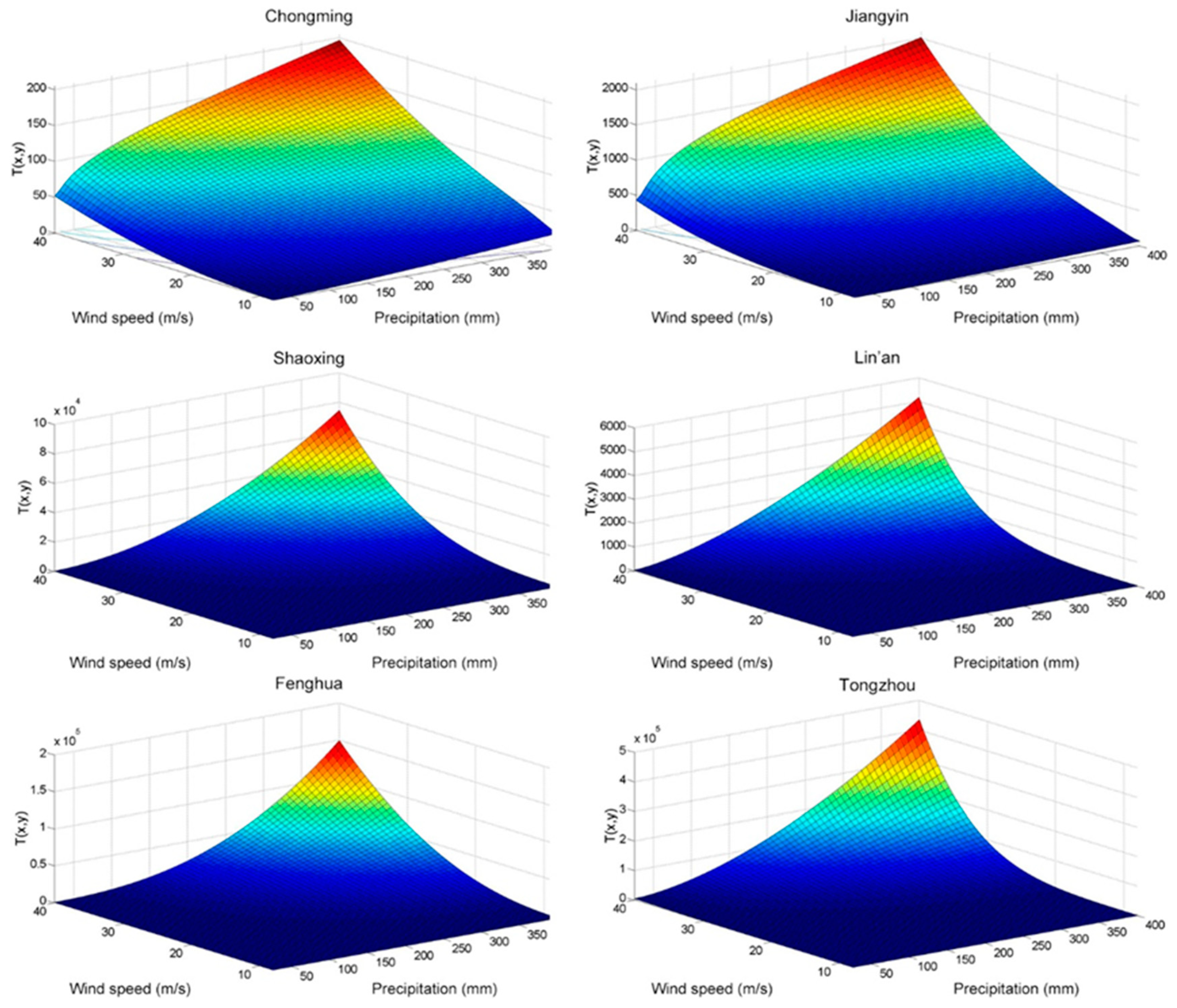
4.2. Vulnerability Analysis

4.2.1. Vulnerability Surface

The estimated value of the coefficients in the trend surface model and the fitted vulnerability surface are shown in

Table 2. The estimated value of the coefficients in the trend surface model.

Parameter	A0	A1	A2	A3	A4	A5
Estimated value (10−6)	−5188.03	222.86	1077.19	−0.31	0.46	8.12

and Figure 5, respectively. The two horizontal axes indicate the intensity of the two hazards, and the vertical axis indicates the loss rate caused by the hazards. Clearly, the loss rate was positively related to the intensity of both hazards.

The coefficient of determination of the trend surface model is denoted by R², the proportion of the regression sum of the square to the sum of the squares of the deviations. The R² value is 0.7339, and the model passes the F-test at the 0.05 significance level. Therefore, the fitted vulnerability surface can effectively denote the intrinsic attribute and be applied in the following risk analysis.

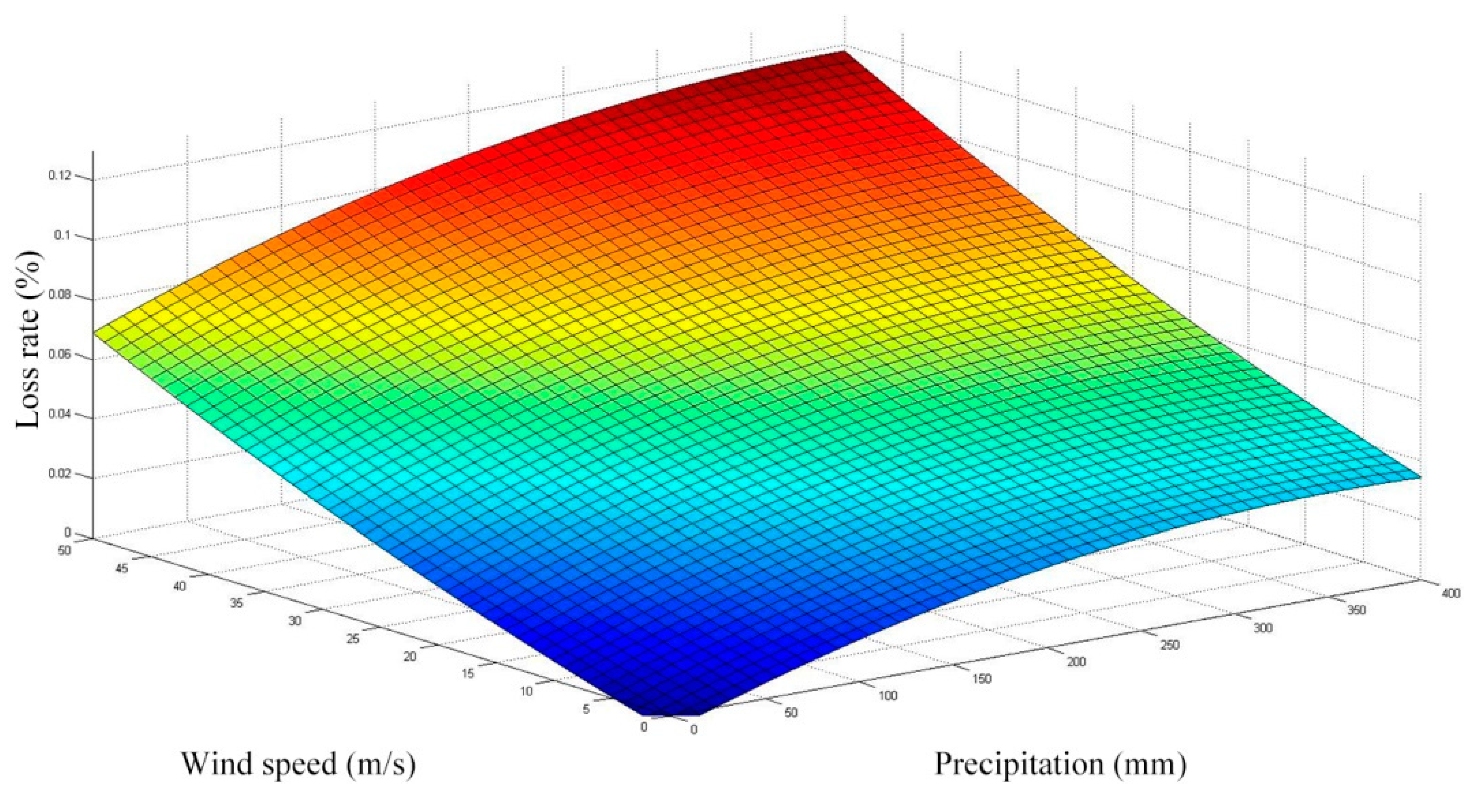
4.2.2. Integrated Vulnerability Model

Table 3. Parameter estimation result of the eightfold linear regression analysis.

Variable	Estimated Value	Standard Error	t-Value	p-Value
Constant	0.03225403	0.01386430	2.32640975	0.02155579
Land area (X1)	−0.00000005	0.00000526	−0.01034332	0.99176335
Crop planting area (X2)	−0.00020566	0.00005626	−3.65557475	0.00037223
Average elevation (X3)	−0.00005530	0.00002225	−2.48517400	0.01422862
Total population (X4)	0.00003522	0.00014548	0.24208981	0.80909502
GDP (X5)	−0.00000049	0.00000036	−1.35049321	0.17922225
GDP per capita (X6)	0.00001312	0.00004715	0.27832100	0.78121158
Total rural machinery power (X7)	0.00000001	0.00000002	0.46568557	0.64222586
Machinery power per square kilometer (X8)	−0.00002247	0.00001741	−1.29055754	0.19916546

shows the estimated values of the parameters in Equation (5). Observably, only the p-values for the constant, X2, and X3 have passed the t-test at the 0.05 significance level. A multivariate linear regression model was rebuilt by removing the factor that had the largest p-value. This step was repeated until all estimated parameters passed the t-test at the 0.05 significance level. The crop planting area, average elevation, and GDP per capita were obtained as the final factors. These results are shown in

Table 4. Parameter estimation result of the threefold linear regression analysis.

Variable	Estimated Value	Standard Error	t-Value	p-Value
Constant	0.02471651	0.00763312	3.23806313	0.00151713
Crop planting area (X1)	−0.00014351	0.00004606	−3.11597140	0.00224336
Average elevation (X2)	−0.00003605	0.00001543	−2.33726150	0.02090731
GDP per capita (X3)	−0.00000043	0.00000016	−2.76799742	0.00643898

Note: Crop planting area is measured in ha, average elevation in meters above the sea level, and GDP per capita in Chinese Yuan per person.

.

The comprehensive vulnerability surface model not only considers the overall internal attributes of a crop but also takes into account the external attributes of a crop determined by the natural and socioeconomic environments of each county in the YRD region. The model presents the relationships among hazard, vulnerability, and potential loss, based on which the risk of crop loss rate of each county can be directly calculated, given the corresponding parameters and variables.

4.3. Risk Assessment Results

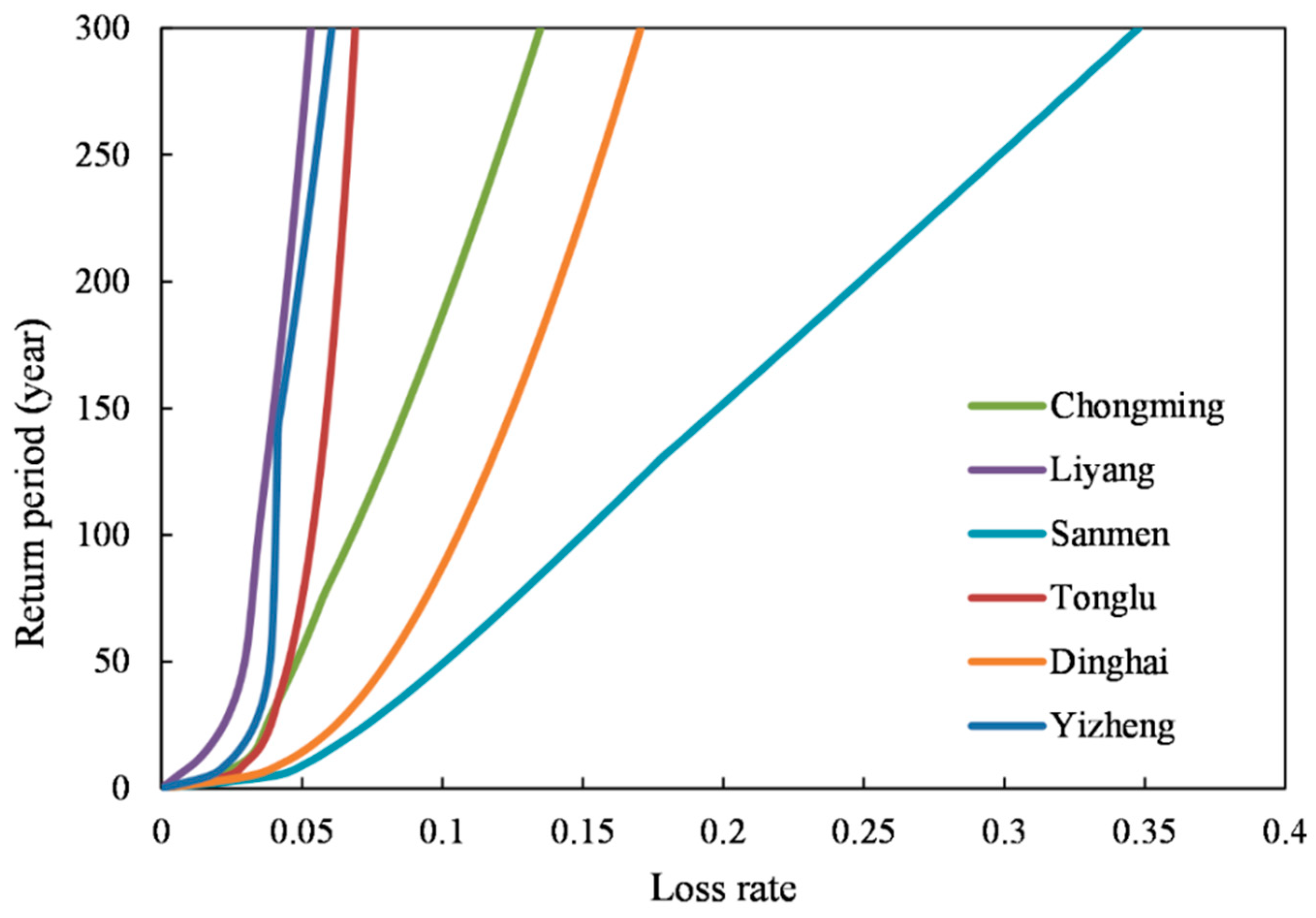
4.3.1. Loss–Return Period Curves

Based on the analysis results of the hazards and vulnerability, the relationship between the return period and the loss rate for 140 counties in the YRD region was individually calculated. Figure 6 shows the loss–return period curves of Chongming in Shanghai; Yizheng and Liyang in Jiangsu; and Tonglu, Dinghai and Sanmen in Zhejiang.

Different patterns for the return period–crop loss rate relationship can be observed in these six counties. With the loss–return period curves, the multi-hazard risk of these counties can easily be compared. Figure 6 and

Table 5. Loss–return period of crops of some counties in the YRD region.

County	Return Period (Year)
	10	20	50	100	150	200
Chongming	0.0286	0.0357	0.0481	0.0679	0.0871	0.1042
Liyang	0.0118	0.0194	0.0296	0.0345	0.0399	0.0449
Yizheng	0.0235	0.0307	0.0387	0.0406	0.0425	0.0491
Tonglu	0.0299	0.0370	0.0454	0.0536	0.0589	0.0630
Dinghai	0.0432	0.0570	0.0804	0.1055	0.1250	0.1417
Sanmen	0.0517	0.0664	0.1009	0.1498	0.1981	0.2486

clearly indicate that Sanmen had the highest disaster risk for crops, followed by Dinghaing, Chongming, Tonglu, and Yizheng. Liyang had the lowest risk. Sanmen, Dinghai, and Chongming, located in coastal areas, were very easily affected by strong wind and flood, while the three interior counties, Tonglu, Yizheng, and Liyang, were less prone to these two hazards. In relation to their geographic location, the risk in coastal areas was higher than that of the central areas, and the risk in the southern areas was higher than that in the northern areas of the YRD region.

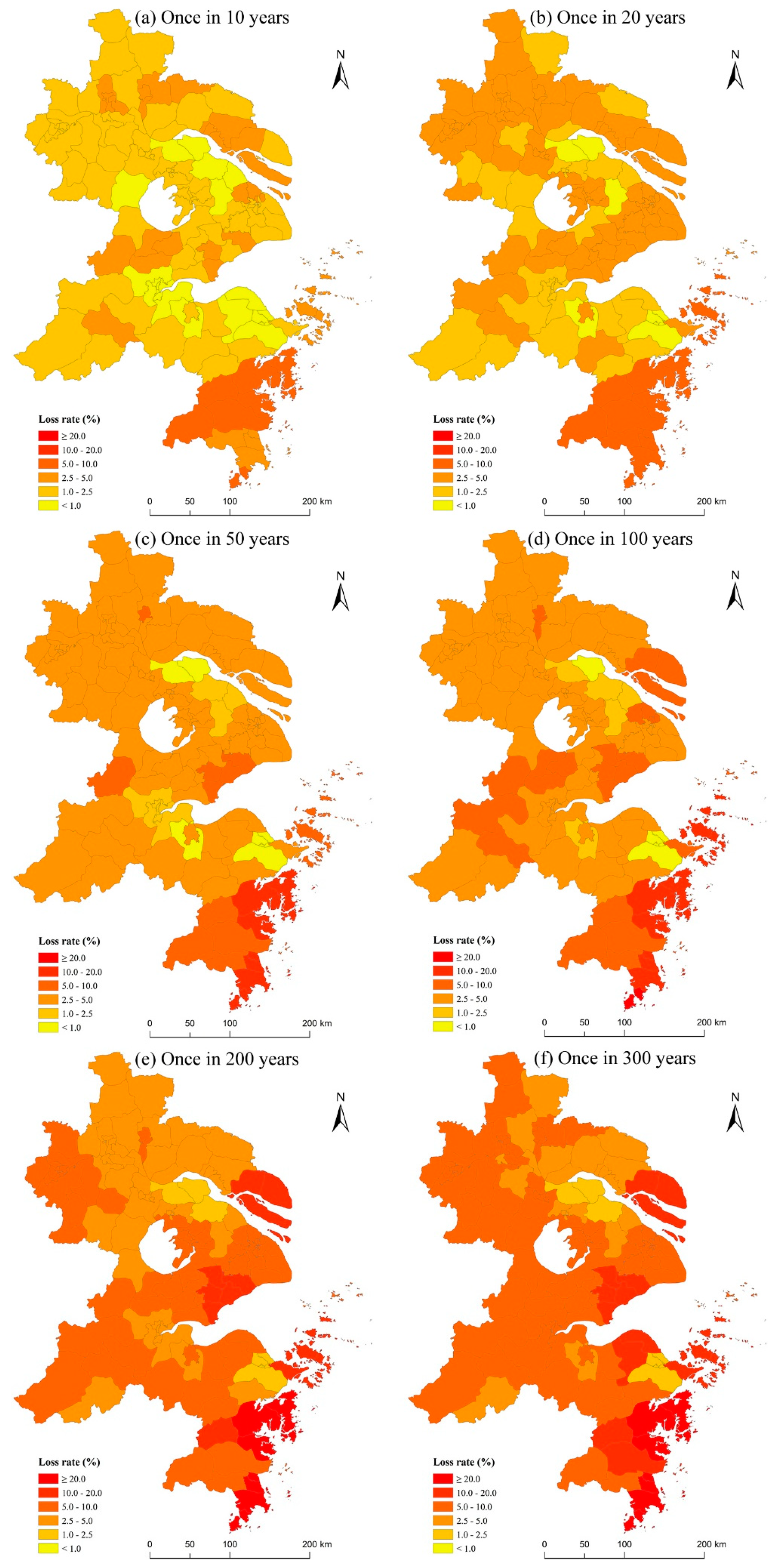
4.3.2. Crop Loss Rate under Different Return Periods

From the loss–return period curve obtained above, the crop loss rate of each county in the YRD region can easily be calculated with a given return period. Figure 7 shows the crop loss rates for six different return periods of each county. Red indicates larger losses, and yellow indicates fewer losses. The crop loss rate of all counties gradually increased with the increase in the return period. For most counties, the loss rates were less than 2.5% when the return period was less than 50 years; they exceeded 2.5% for 200 years and were more than 5% for 300 years. In terms of geographical distribution, the counties in the southeastern areas of the YRD region had a higher crop loss risk than those in the northwest. For example, Taizhou and Zhoushan had the highest crop loss risk, followed by Chongming, Jiaxing, Qidong, and Shanghai.

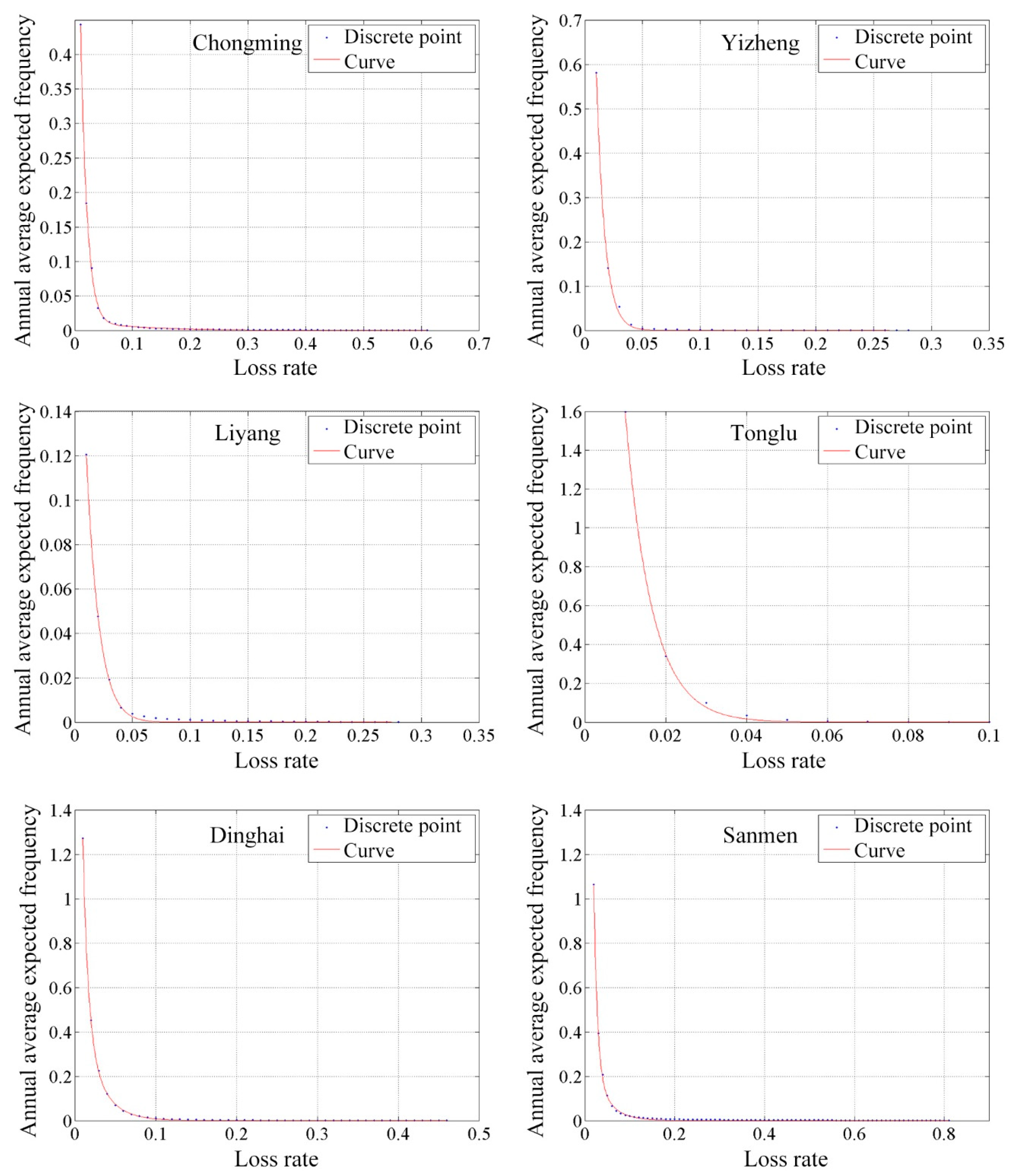
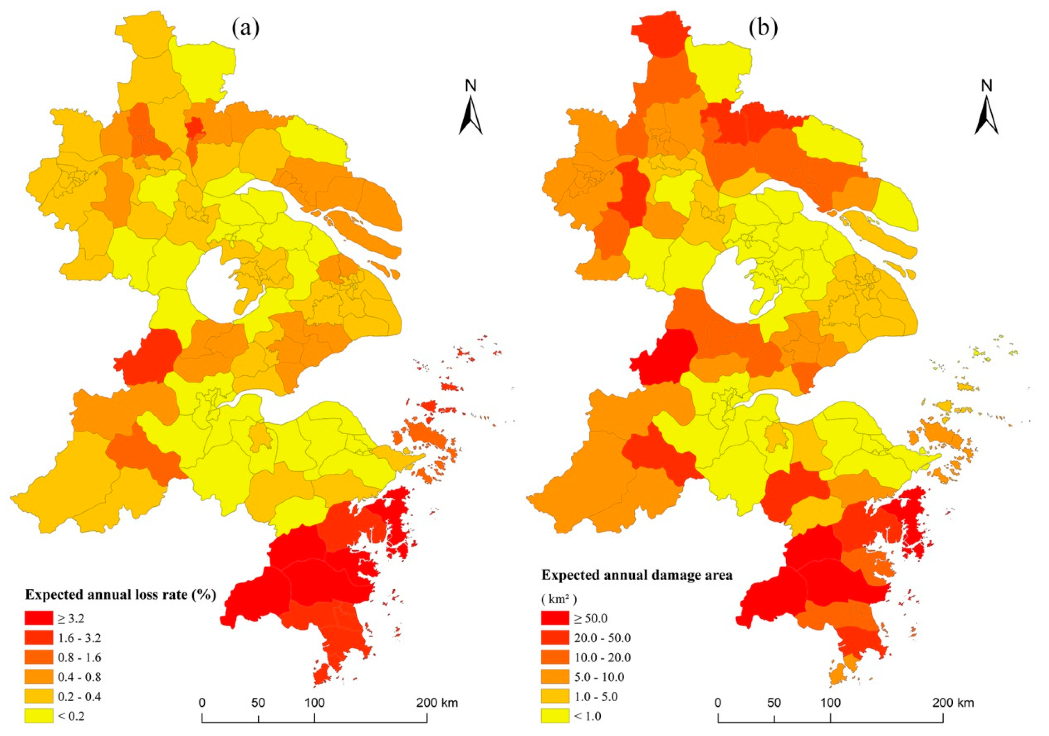
4.3.3. Annual Average Frequency of Losses and the Annual Average Expected Losses

The crop loss rate-average annual frequency curve was fitted using a Gaussian function for each county in the YRD region, and the goodness-of-fit R² values for all counties were greater than 0.99. Figure 8 shows the fitted result for Chongming, Yizheng, Liyang, Tonglu, Dinghai, and Sanmen. The horizontal axis indicates the crop loss rate, and the vertical axis indicates the annual average expected frequency. The greater the loss, the lower the expected frequency of occurrence. The risk can be judged from the area enclosed by the curve and the coordinate axis. Sanmen County has the highest risk, and Liyang City has the lowest risk.

The annual average expected loss rate and expected annual damage area are a more explicit expression of the risk of crop loss. The annual average expected loss rate and expected annual damage area of each county in the YRD region are shown in Figure 9. Evidently, the counties in the Taizhou and Ningbo Prefectures, which are located in the southeastern coastal area of the YRD region, have the highest annual average expected loss rate. They are followed by the counties in the Zhoushan, Jiaxing, and Huzhou Prefectures and Chongming and the counties in Nantong Prefecture. The zonal characteristics of loss are generally greater in the south than in the north, but their regional differences are not as obvious as those for the joint hazard.

5. Conclusion and Discussion

In this study, the crop loss risks due to the multiple natural hazards of heavy rain and strong wind were quantitatively assessed based on a copula method and vulnerability surface in the YRD region of China. To obtain the relationship between the two hazards, a copula function was first applied to calculate their joint probability distribution and return period. The trend surface analysis was applied to build a vulnerability surface model that reflected the internal attributes of exposure. Then, multiple regression analysis was used to screen out the significant variables that reflect external attributes, based on which an integrated vulnerability model was developed. The results show that the vulnerability surface is well fitted, considering the joint hazards of rainfall and strong wind and the sown area of crops, average elevation, and GDP per capita. There is clear regional heterogeneity in the joint probability distributions and crop loss risks of heavy rain and strong wind in the YRD region. The counties in the southeast coastal areas have a higher joint probability and higher risks than those in the central region, and the south has a higher joint probability and higher risks than the north. The coastal area of Taizhou in the southeast has the highest risk of crop loss, followed by Huzhou and Jiaxing in the middle and Chongming, Tongzhou, and Yizheng in the north.

Notably, there have been several other methods to quantitatively calculate the total risk of multiple hazards, such as using the information diffusion [14,19], the independent distribution method [17,18], directly summarizing the risks of each individual hazard [13], and the weighted method [8,9,10]. The calculation procedure is relatively easier compared with to the copula method, especially for the total risk of more than three hazards. All hazards are assumed to be independent—that is to say, the interactions between the different hazards are not considered in these models. In the reality, several hazards may take place at the same time, and some of them do not occur alone or they may be dependent. In these cases, the total loss or risk cannot be summarized by using weighted method or the independent distribution method to combine the loss or risk from each individual hazard. The copula function is a useful method to calculate the joint loss or risk if the hazards are dependent. It should be noted that the copula function is also useful for calculating the joint probability distribution or joint return period of three or more dependent hazards, although the procedure will be more complicated [20]. However, the method is be difficult to use in calculating the total risk of three or more types of hazards due to lack of enough historical pair data of loss and hazard to fit the vulnerability. By generating more pair data with experiments and computer simulations, the method will be gradually used for quantitatively assessing the integrated risk of three or more types of dependent hazards.

It has been mentioned that although we have found 162 sets of hazard–loss data for vulnerability fitting, the losses may also include the average fluctuation of crop loss. Understanding how to use integrated bio-economic simulation models to extract the expected fluctuation from crop loss risk would be necessary to make the risk assessment result more sophisticated. Climate change may affect the frequency, intensity, duration, tendency, and fluctuation of precipitation and wind, but this issue was not considered in this study. In addition, changes in exposure and the factors that affect the external attributes were not considered when calculating the crop loss risk in this study. For example, with economic and technological development, the vulnerability of crops to hazards might also decrease, which will definitely reduce possible losses. Integrating analysis that considers climate change, exposure, and vulnerability into the proposed model may be a solution to these problems.

References

1. United Nations. Transforming Our Word: The 2030 Agenda for Sustainable Development; United Nations: New York, NY, USA, 2015. [Google Scholar]
2. Gill, J.C.; Malamud, B.D. Reviewing and visualizing the interactions of natural hazards. Rev. Geophys. 2014, 52, 680–722. [Google Scholar] [CrossRef] [Green Version]
3. Pelling, M.; Maskrey, A.; Ruiz, P.; Hall, L. Reducing Disaster Risk: A Challenge for Development; UNDP, United Nations Development Programme: New York, NY, USA, 2004; pp. 113–115. ISBN 92-1-126160-0. [Google Scholar]
4. Dilley, M.; Chen, R.S.; Deichmann, U.; Lerner-Lam, A.L.; Arnold, M.; Agwe, J.; Buys, P.; Kjekstad, O.; Lyon, B.; Yetman, G. Natural Disaster Hotspots: A Global Risk Analysis; The World Bank: Washington, DC, USA, 2005; pp. 1–132. ISBN 0-8213-5930-4. [Google Scholar]
5. UNU-EHS (United Nations University Institute for Environment and Human Security). World Risk Report; Bündnis Entwicklung Hilft: Berlin, Germany, 2013; ISBN 978-3-9814495-3-2. [Google Scholar]
6. Schmidt-Thomé, P. The Spatial Effects and Management of Natural and Technological Hazards in Europe—ESPON 1.3.1; European Spatial Planning Observation Network Monitoring Committee: Luxembourg, 2006; pp. 1–197. ISBN 951-690-918-3. Available online: https://www.espon.eu/sites/default/files/attachments/fr-1.3.1_revised-full.pdf (accessed on 25 December 2018).
7. JRC (European Commission Joint Research Centre). Index for Risk Management—INFORM; Publications Office of the European Union: Luxembourg, 2015. [Google Scholar]
8. Shi, P.; Yang, X.; Liu, F.; Li, M.; Pan, H.; Yang, W.; Fang, J.; Sun, S.; Tan, C.; Yang, H.; et al. Mapping Multi-hazard Risk of the World. In World Atlas of Natural Disaster Risk; Shi, P., Kasperson, R., Eds.; Springer: Heidelberg/Berlin, Germany, 2015; ISBN 978-3-662-45430-5. [Google Scholar]
9. Shi, P.; Yang, X.; Fang, J.; Wang, J.; Xu, W.; Han, G. Mapping and ranking global mortality, affected population and GDP loss risks for multiple climatic hazards. J. Geogr. Sci. 2016, 26, 878–888. [Google Scholar] [CrossRef]
10. Shi, P.; Yang, X.; Xu, W.; Wang, J. Mapping Global Mortality and Affected Population Risks for Multiple Natural Hazards. Int. J. Disaster Risk Sci. 2016, 7, 54–62. [Google Scholar] [CrossRef] [Green Version]
11. UNISDR (United Nations International Strategy for Disaster Reduction). From Shared Risk to Shared Value: The Business Case for Disaster Risk Reduction; Global Assessment Report; Disaster Risk Reduction (GAR): Geneva, Switzerland, 2013; ISBN 978-92-1-132038-1. [Google Scholar]
12. UNISDR (United Nations International Strategy for Disaster Reduction). Making Development Sustainable: The Future of Disaster Risk Management; Global Assessment Report; Disaster Risk Reduction (GAR): Geneva, Switzerland, 2015; ISBN 978-92-1-132042-8. [Google Scholar]
13. UNISDR (United Nations International Strategy for Disaster Reduction). The GAR Atlas: Unveiling Global Disaster Risk; Disaster Risk Reduction (GAR): Geneva, Switzerland, 2017. [Google Scholar]
14. Xu, W.; Tian, Y.; Zhang, Y.; Zheng, J.; Fang, W.; Lv, H.; Yang, X.; Wang, R.; Zhao, T.; Shi, P. Integrated Risk Governance: Natural Hazards and Risk Assessment in the Yangtze River Delta Region; Science Press: Beijing, China, 2014. (In Chinese) [Google Scholar]
15. Xu, W.; Zhuo, L.; Zheng, J.; Ge, Y.; Gu, Z.; Tian, Y. Assessment of the Casualty Risk of Multiple Meteorological Hazards in China. Int. J. Environ. Res. Public Health 2016, 13, 222. [Google Scholar] [CrossRef] [PubMed]
16. Kappes, M.S.; Keiler, M.; von Elverfeldt, K.; Glade, T. Challenges of analyzing multi-hazard risk: A review. Nat. Hazards 2012, 64, 1925–1958. [Google Scholar] [CrossRef]
17. Ordaz, M. A simple probabilistic model to combine losses arising from the simultaneous occurrence of several hazards. Nat. Hazards 2015, 76, 389–396. [Google Scholar] [CrossRef]
18. Bernal, G.A.; Salgado-Ga´lvez, M.A.; Zuloaga, D.; Tristancho, J.; Gonza´lez, D.; Cardona, O. Integration of Probabilistic and Multi-Hazard Risk Assessment Within Urban Development Planning and Emergency Preparedness and Response: Application to Manizales, Colombia. Int. J. Disaster Risk. Sci. 2017, 8, 270–283. [Google Scholar] [CrossRef] [Green Version]
19. Liu, B.; Siu, Y.L.; Mitchell, G.; Xu, W. Exceedance probability of multiple natural hazards: Risk assessment in China’s Yangtze River Delta. Nat. Hazards 2013, 69, 2039–2055. [Google Scholar] [CrossRef]
20. Ming, X.; Xu, W.; Li, Y.; Du, J.; Liu, B.; Shi, P. Quantitative multi-hazard risk assessment with vulnerability surface and hazard joint return period. Stoch. Environ. Res. Risk Assess. 2015, 29, 35–44. [Google Scholar] [CrossRef]
21. Li, N.; Liu, X.; Xie, W.; Wu, J.; Zhang, P. The return period analysis of natural disasters with statistical modeling of bivariate joint probability distribution. Risk Anal. 2013, 33, 134–145. [Google Scholar] [CrossRef] [PubMed]
Figure 1. The YRD region.
Sustainability 11 00922 g001
Figure 2. The joint probability distributions of heavy rain and strong wind for some counties in the YRD region.
Sustainability 11 00922 g002
Figure 3. The joint return period distribution of strong wind and heavy rain for some counties in the YRD region.
Sustainability 11 00922 g003
Figure 4. The joint return period of wind and rain hazards at different intensity ranks.
Sustainability 11 00922 g004
Figure 5. The vulnerability surface based on the intrinsic attributes of exposure.
Sustainability 11 00922 g005
Figure 6. Loss–return period curves of some counties in the YRD region.
Sustainability 11 00922 g006
Figure 7. Crop loss rate under different return periods for each county of the YRD region.
Sustainability 11 00922 g007
Figure 8. Annual frequency curves of the loss rate in some counties in the YRD region.
Sustainability 11 00922 g008
Figure 9. The (a) expected annual loss rate and (b) expected annual damage area of crops for each county in the YRD region.
Sustainability 11 00922 g009