The Effect of Land Use on Housing Price and Rent: Empirical Evidence of Job Accessibility and Mixed Land Use

1
Department of Landscape Architecture, Seoul National University, 1 Gwanak-ro, Gwanak-gu, Seoul 08826, Korea
2
Department of Real Estate, Graduate School of Tourism, Kyung Hee University, 26 Kyungheedae-ro, Dongdaemun-gu, Seoul 02447, Korea
*
Author to whom correspondence should be addressed.
Sustainability 2019, 11(3), 938; https://0-doi-org.brum.beds.ac.uk/10.3390/su11030938
Submission received: 18 December 2018
/
Revised: 1 February 2019
/
Accepted: 9 February 2019
/
Published: 12 February 2019
(This article belongs to the Section Sustainable Urban and Rural Development)
Abstract
:Recently, the improvement of job accessibility and the encouragement of mixed land use have been gaining popularity in the planning field. However, little is known about whether these two factors are able to meet housing consumers’ needs. This study aims to analyze how job accessibility and mixed land use satisfy housing consumers’ needs. Particularly, this study investigates housing consumers’ willingness to pay for these two features by using housing prices and rents in the Chicago metropolitan area. In order to deal with endogeneity between land use and housing prices and spatial autocorrelation between housing prices, spatial econometric models are used with instrumental variables. Interestingly, our findings show that an increase in job accessibility leads to an increase in housing prices, whereas it is not related to rents. We also found that mixed land use decreases housing prices, but increases rents.
1. Introduction
Today’s land use planning and policies are intended to preserve values of cultural resources and enhance sustainable communities and neighborhoods. Among various specific components to achieve these goals in planning practice, the improvement of job accessibility and the encouragement of mixed land use have gaining popularity in the planning field. This is because successfully designing and utilizing these two features through land use and transportation planning not only can reduce individual vehicle mile travel (VMT) and urban traffic congestion [1] but can also provide lively urban environments [2]. In addition, both higher job accessibility and mixed land use have been considered as signature features of smart growth, because increasing these two components makes more workers live near their workplaces. Living closer to jobs and locating closer to workers would have great benefits for workers as well as employers by reducing commuting costs and making employers easier to find. However, although these two elements improve the balance of jobs and housing, they are different in other ways. For example, job accessibility is a global concept encompassing an entire city [3,4], while mixed land use is a local concept related to neighborhoods [5]. Hence, they may have different socioeconomic impacts, and should be differently and carefully investigated. However, few studies have examined the differences between these two concepts in housing markets.
In past decades, numerous studies have provided empirical evidence of their effectiveness; for example, a reduction of the physical distance between jobs and housing through these two components increases public transportation use, walking, and bicycling [6]. However, little attention has been paid to the demand side of the land use components. Particularly, little is known about which land use features are more important for different demanders. Previous studies have shown that different age groups or different income groups have different preferences regarding their residential locations [7,8]. That is, while some people prefer locations closer to jobs, others choose locations relatively far from their workplaces. For example, single young groups prefer downtown or employment sub-centers because these places provide better urban amenities such as cafés, restaurants, museums, or shopping centers, while households with children prefer single-family housings or neighborhoods with higher safety, better schools, or better natural amenities [8]. In addition, scholars have recently pointed out that rental markets have significantly different characteristics in the US housing markets [9], which suggests that in-depth analysis is necessary for understanding the relationship between housing submarkets and demanders’ needs (i.e., housing demanders and renters). Nevertheless, our understanding of whether land use features really meet residents’ needs is still limited.
Some scholars have pointed out that most previous studies have only focused on supply-oriented policies or planning [10,11]. Using smart growth features, policy makers have tried to reduce vehicle use and encourage walking and biking commutes. However, in order to create sustainable urban places and better living environments given the limited amount of urban land, land use planning or policies carefully reflecting demanders’ needs are essential. Koster and Rouwendal [10] argued that the preferences of residents or housing consumers should be carefully considered in land use planning, because their preferences do not play a role in decisions of local government. If housing consumers do not respond to the contemporary land use policies (e.g., Smart Growth or New Urbanism), the planning strategies are not desirable. In contrast, if they have a willingness to pay for mixed land use or land use with higher job accessibility, such policies would be appropriate as well as economically effective.
Hence, an investigation of the impacts of key land use features is necessary for suggesting implications for future land use planning. Traditionally, housing demanders’ preferences can be identified through survey or interview by asking them if they want to live near neighborhoods with higher mixed land use or better job accessibility [12]. However, because of limitations of survey data collection, it can also be indirectly captured by demanders’ willingness to pay for housing prices or rents. For example, if land use with high job accessibility and well-mixed activities increases housing values or rent prices, housing consumers are regarded as preferring those land use planning [11]. On the other hand, if such land use elements do not increase housing values, housing consumers are regarded as having no preference for the land use features. Although previous studies have examined their relationships, it remains to be seen which land use features are more related to housing prices or rents. Additional empirical research is necessary to fill this gap.
Taking this into perspective, the objective of this study is to examine whether housing consumers prefer mixed land use and higher job accessibility. Particularly, we focus on housing consumer’s willingness to pay for housing values in the Chicago metropolitan area. This study has three unique contributions. First, we attempt to use an appropriate index for mixed land use and job accessibility. Job accessibility and mixed land use can be measured differently by different researchers. Therefore, employing a more proper method to calculate the index is important to figure out its impact. Second, we compare whether housing consumers’ and renters’ land use preferences are the same. Since they have different socioeconomic characteristics with respect to income or age, we presume that they have different preferences. Third, we consider an endogeneity issue occurring between housing prices and land use as well as spatial autocorrelation between housing prices. For example, while higher job accessibility and higher mixed land use are likely to affect housing prices, higher housing prices also can affect job accessibility and mixed land use development simultaneously. In addition, housing prices are generally affected by neighboring housing prices or neighboring unobserved characteristics. Therefore, this relationship should be carefully considered in the estimation of parameters.
This study is organized into six sections, including this introduction. Following this introduction, the next section represents literature reviews relevant to land use and housing prices by focusing on job accessibility and mixed land use. In Section 3, study area and data are presented. Section 4 explains a methodological framework to examine the effects of job accessibility and mixed land use on housing prices. Section 5 provides empirical evidence of the relationship between land use and housing prices. In Section 6, we discuss our findings and suggest policy implications.
2. Literature Review
Although a number of studies on the effects of neighborhood spatial characteristics on housing prices have been conducted, little is understood about how the two important land use features related to smart growth strategies—mixed land use and job accessibility—influence housing prices and rents, respectively. In other words, few studies have examined which one is more important for increasing housing and/or rent prices that reflect housing demanders’ preferences. Because housing market consists of different sub-markets (e.g., rental markets and housing markets), housing prices and rental prices should be differently investigated for efficient land use policies [9]. Previous studies have shown that renters and housing buyers have different preferences [13]. Generally, low-income households choose rental housing, but middle- or high-income households prefer single-family housing units. Also, this can vary by different age groups; sometimes young adults choose high price rental housings that are located downtown because they prefer neighborhoods that provide urban amenities such as cafés, museums, restaurants, and shopping centers [8].
There are two possible reasons of lack of these studies. First, there is no definitive measurement of these two land use components. Scholars have focused more on an appropriate way to measure these land use characteristics. For example, different measurements have been applied in different previous studies [10,11,14,15,16]. Second, as mentioned above, most previous studies on land use planning have disregarded consumers’ preferences focused on supply-oriented sides. For example, while numerous studies have examined the effects of land use on sustainable commuting patterns, especially focusing on travel behaviors and commute distance [1,15,16,17], there have been relatively few empirical studies supporting that these land use patterns really meet housing consumers’ needs. In this section, we review two research issues regarding job accessibility and housing prices, and mixed land use and housing prices, by focusing on the empirical research as well as methodological approaches for measurement of job accessibility and mixed land use index.
2.1. Job Accessibility Measures
Scholars in the urban planning field have long recognized the relationship between accessibility and property values. They have used a hedonic price model developed by Rosen [18] to investigate the relationship between accessibility and property values by controlling for other factors. The hedonic price model explains the composition of housing prices by disentangling the bundle of housing services, and accessibility is one of the most important spatial characteristics explaining housing prices. A number of studies have used the hedonic price model to explore the effect of accessibility on housing values. For example, scholars have considered accessibility to rail station [19,20], actual ridership level [21], and system street network connectivity [22] as determinants of housing prices. However, the concept of accessibility, which is measured by distance to bus stops or light rail stations, cannot deal with entire levels of urban traffic congestion or traffic speed caused by the spatial distribution of population and employment, because the accessibility measures do not account for where people go and where they come from.
According to the urban economic theory, the study of the relationship between job accessibility and housing prices has been developed by Alonso’s [23] monocentric model, which explains residential activities are determined by a tradeoff between the accessibility of being close to the central business district (CBD) and property values. This theory has been further developed by Muth [24] and Mills [25], and the concept of accessibility has been measured by distance from the CBD. However, as employment began to disperse from central cities to suburban areas, diverse polycentric models emphasizing the importance of employment subcenters have been suggested [26,27,28]. In reality, large population and employment subcenters have emerged outside of central cities in large metropolitan areas. As a result, major cities have become increasingly polycentric. This phenomenon has been driven by job clusters that emerge where there is a good transportation network and suburbanization of labor force [27]. Therefore, accessibility is no longer simply measured by distance to the CBD.
Alternatively, various accessibility measures have been developed by several scholars for investigating the effects of multiple centers. For example, Hansen [29] first developed a gravity model to measure job accessibility. Noland [30] used simple job accessibility using total jobs across employment centers weighted by the inverse of distance to each center. Waddell [31] used job accessibility measured by travel time instead of distance. Shen [3] suggested a refined gravity-based model by arguing that job accessibility should be measured with consideration of the composition of employment by occupation and industry. The refined gravity-based model has recently been used in some studies that show its applicability and usefulness [15,32]. In addition, scholars have used the gravity-based labor market accessibility that deals with polycentric tendencies in the spatial structure [3,32,33]. For example, Osland and Thorsen [32] showed that this gravity-based labor market accessibility considering spatial distribution of population and employment can explain spatial variations of housing prices. Jin and Paulsen [34] have shown that this refined gravity-based accessibility measure is appropriate to examine the relationship between job accessibility and labor market outcomes. Although its applicability has been proved in several examples of research, it has not been used to investigate its effect on housing prices. We employ the refined gravity-based model in our research, which will be explained in detail in Section 4.
2.2. Mixed Land Use and Housing Price
The concept of mixed land use has been raised by the New Urbanism movement. Since the 1960s, U.S. zoning ordinances have regulated land use development by isolating commercial, industrial, shopping, and services employment from residential housing, which has resulted in residential neighborhoods being developed separately from jobs and services. Scholars have argued that the spatial separation of jobs and housing causes traffic congestion, air pollution, and inefficient energy consumption. As an alternative method of land use development, it is argued that mixture of complimentary land use types including housing, service, office, industrial use, and retail will provide significant benefits in solving these problems.
Although the claims of mixed land use have been a starting point to generate numerous studies examining the effects of mixed land use on commuting patterns, only a few studies have investigated the effects of mixed land use on housing prices. Cao and Cory [35] addressed the importance of the relationship between mixed land use and residential property values. Using the hedonic regression model accounting for the reverse causality between mixed land use and housing values, Song and Knaap [14,36] showed that housing prices are higher in neighborhoods dominated by single-family residential land use, while housing prices decrease with proximity to multi-family residential units. Mattews and Turnbull [22] found that the effects of mixed land use on housing prices depend on development characteristics of neighborhoods. For example, while there is a positive effect of mixed land use on housing prices in pedestrian-oriented neighborhoods, there is no significant effect in automobile-oriented neighborhoods.
More recently, Koster and Rouwendal [10] investigated how households value mixing of housing and jobs, focusing on the Rotterdam city region. They found that mixed land use increases housing prices. For example, households are willing to pay about 2.5 percent more for a house located in a neighborhood with mixed land use. They also compared the effect of mixed land use on housing prices of single-family housing and apartments. Their findings demonstrated that apartment occupiers are willing to pay for mixed land use development, whereas households living in a single-family housing are not willing to pay for mixed land use development. Moreover, with his theoretical discussion of the effects of mixed land use on the quantity of affordable housing, Aurand [37] provided evidence that neighborhoods with a greater variety of housing types and residential density offer a greater quantity of affordable housing for low-income renters. He suggested that planners and policy makers should specify the goals of housing types.
In sum, although mixed land use development and efforts for providing better job accessibility through urban planning have been conducted, little attention has paid to the relationship between the two features and housing prices. Particularly, little is known about which one is more related to housing prices or rents. If planners want to make a sustainable community through the mixed land use development and integration of jobs and housing in a neighborhood, more investigations regarding how housing consumers feel about the two components are necessary. Particularly, exploring the effect of land use on housing prices differentiated by characteristics could have important policy implications.
3. Study Area and Data
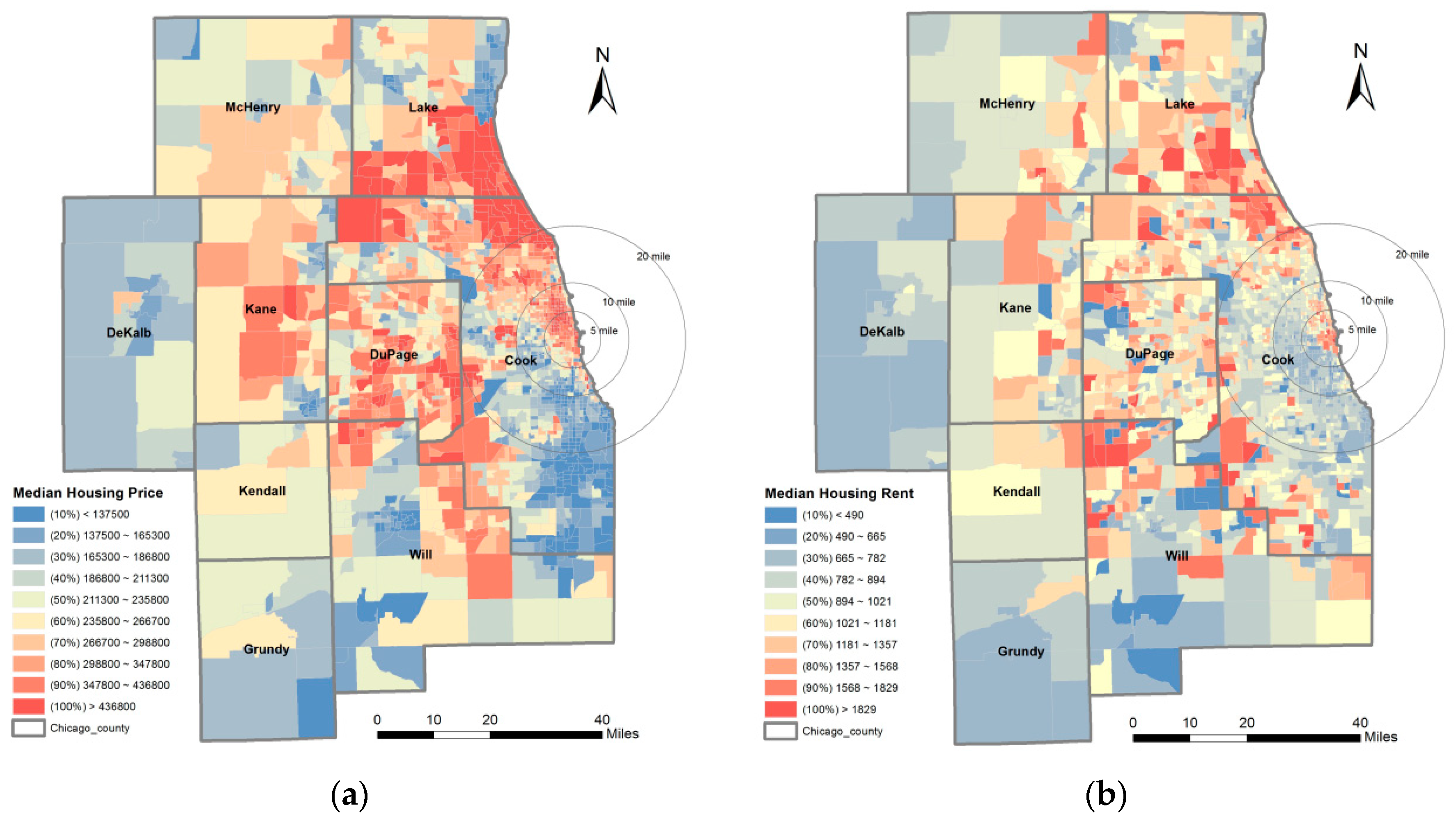
Our study area is the Chicago metropolitan area, including nine counties such as Cook, DuPage, Lake, McHenry, Kane, DeKalb, Kendall, Grundy, and Will. We use various datasets. Specifically, we use median housing price and median rent in 2009–2013 ACS (American Community Survey). Figure 1 shows the spatial distribution of the housing prices and rents in the Chicago metropolitan area. The housing prices in the northern part of Chicago are relatively higher than those in the southern part. The spatial distribution of rent prices looks little different from that of housing prices, but rent prices in the northern part of Chicago are relatively higher, which is similar to the distribution of housing prices. Additionally, we obtain other data, such as housing characteristics, household characteristics, and socio-economic characteristics by census tracts from 2009–2013 ACS. In order to measure the index for mixed land use and job accessibility, we use 2013 LEHD (Longitudinal Employer-Household Dynamics) LODES data. The LEHD data provide spatial information on the employees’ work places and residential locations at the census block level, which allows us to combine LEHD with ACS at the census tract level. Hence, we first aggregate the LEHD at the census tract level, and combine LEHD and ACS, and then calculate job accessibility and mixed land use indices based on the equations explained in the next section.
4. Methodology
4.1. Analytical Framework(Generalized Spatial Two-Stage Least Square: GS2SLS)
Hedonic price model has been developed and widely used to identify the factors explaining housing prices [38]. In this study, we deal with additional two statistical issues: endogeneity between land use and housing price, and spatial autocorrelation between housing prices. First, endogeneity should be carefully accounted for when measuring the effect of land use on housing prices because a simultaneous relationship between land use and housing prices exists. For example, better accessibility or high levels of mixed land use increase housing prices because such land use features bring about more activities—firms are encouraged to move in, and thus more facilities are constructed. This increases the housing demand in surrounding areas, and thus raises housing prices. This relationship can be expressed as the following equation:
where denotes housing prices, L denotes land use characteristics, X denotes exogenous factors affecting housing prices, and denotes error terms. However, as the land use characteristics affect housing prices, the increased housing prices simultaneously bring about more demand for development. Thus, increased housing prices lead to increased commercial development. This relationship can be expressed as the following equation:
In order to account for endogeneity, instrumental variables can be used. The instrumental variables are associated with land use characteristics (L), but are not related to the error term () in Equation (1). Generally, two-stage least square (2SLS) estimator is used when estimating the parameter using instrumental variables. In the first step, we estimate the expected values of land use using instrumental variables with control variables, and then we estimate the empirical housing price model, which is depicted as follows:
- First-stage
- Second-stage
Through the instrumental variables with 2SLS, we can control for endogeneity. However, this approach cannot deal with spatial autocorrelation between housing prices. Previous studies have demonstrated that housing prices can be spatially affected by neighboring housing prices or unobserved neighboring factors. If we do not control for spatial autocorrelation, the estimated values can be biased and inefficient [39]. In order to account for this issue, we use generalized spatial two-stage least square (GS2SLS) model that accounts for endogeneity and spatial autocorrelation together, which is expressed as the following equations:
Because the hedonic price model generally uses a log form of housing prices, our final empirical model used in this study is expressed as the following equations:
A spatial weight matrix presents the pairwise spatial relationship between two any spatial units. It has two different types such as contiguity-based weight matrix and distance-based weight matrix. We simply use the contiguity-based weight matrix, which is measured by the queen criterion.
4.2. Measurement of Variables
4.2.1. Job Accessibility
Among the various job accessibility measures, Hansen’s [18] gravity-based model has been widely used. The basic gravity-based model is as follows:
where denotes job accessibility index in census tract i, denotes the number of employment in census tract j, denotes an impedance parameter, and denotes the distance between census tract i and j. The main advantage of the gravity-based model is that it provides a simple and accurate single parameter measurement of actual commuting patterns [33]. However, Shen [3] argued that demand potential should be accounted for when measuring job accessibility because job opportunities are differentiated between locations with different levels of demand potential. He suggested the formulation of refined gravity-based model as follows:
where denotes demand potential in a location j, and denotes the number of people in location k seeking the job opportunities, k = 1, 2, …., N. In this equation, potential job seekers are defined as persons 18–64 years old. This refined accessibility model has been employed in current several studies [4,32] and proved its applicability (see [34]). Hence, we measure job accessibility based on Equation (8). An impedance function using an empirically derived impedance coefficient enables the formula to assign a lower weight to jobs located farther from the household residential location. In this study, distance is bound to incorporate only the interzonal pair for which distances are less than 45 miles since the attractiveness of employment opportunities declines as travel distance or time increases [33]. Recently, Hu [3] estimates a decay parameter of 0.105 for Chicago, which is based on 2000 Census Transportation Planning Package (CTPP) Part 3 data. We employ Hu’s parameter to calculate the job accessibility.
4.2.2. Mixed Land Use
There is no definitive way to measure mixed land use, and it has been differently measured among researchers. Previous studies have frequently used the concept of entropy as a mixed land use index, which captures the diversity degree of land use within a certain area. Particularly, Song and Knaap [14] measured the mixed land use index based on the concept of entropy by considering the proportion of areas by land use types. For example, if the mixed land use index is equal to 1, it means only single type land use exists in the location. In contrast, the value of 0 in the mixed use index indicates that all types of land use have equal proportions in the given area. The equation is as follows:
where H denotes the mixed land use index, S denotes the number of land use types, and P denotes the proportions of each of the land use types. However, this index does not tell what kinds of activities are really performed in a given area. Moreover, it is not easy to obtain land use data including all types of land use in a specific time period. Alternatively, others used mixed land use index measured by the number of households and the number of employees in every sector [10,40]. Koster et al. [10] and Duranton et al. [40] have pointed out that mixed land use can be measured based on the combination of different employment sectors with residential units, and this index can be compatible with mixed land use. The index is based on the Hirshmann–Herfindahl index and the equation is as follows:
where
denotes the mixed land use index for house h, which is defined as the inverse of the Hirschmann-Herfindahl index; denotes the number of households in a neighborhood of house h; and denotes the number of employees in sector g. If there are employees of only one sector in a certain area, is equal to 1. Additionally, if economic activities become more diverse in the area, the mixed land use index goes up. Although this index does not show which types of mixed land use exist in a certain area, it shows how much different employment sectors based on the 20 NACIS codes (e.g., retail, manufacturing, real estate, etc.), including residential units, exist in a certain area. In this study, we adopted the formulation of the latter.
4.2.3. Instrumental Variables
As described in the analytical framework, we use instrumental variables to account for endogeneity occurring between housing prices and land use characteristics. Applicability of the instrumental variables that are associated with land use characteristics but not related to error term should be supported theoretically and statistically. We emulate previous studies that have used instrumental variables [14]. Specifically, we use two instrumental variables—distance to the major roadways (including every interstate highway, state highways, and arterial roadways) and distance—to subcenters. These two variables are exogenous, but they are not correlated with job accessibility and mixed land use since they potentially influence the spatial distribution of jobs [34]. In general, firms are likely to locate near major roadways and subcenters for reducing transportation costs and obtaining the benefits of agglomeration economies. Empirical studies have demonstrated the relationship between job growth and the location of subcenters [27,41,42].
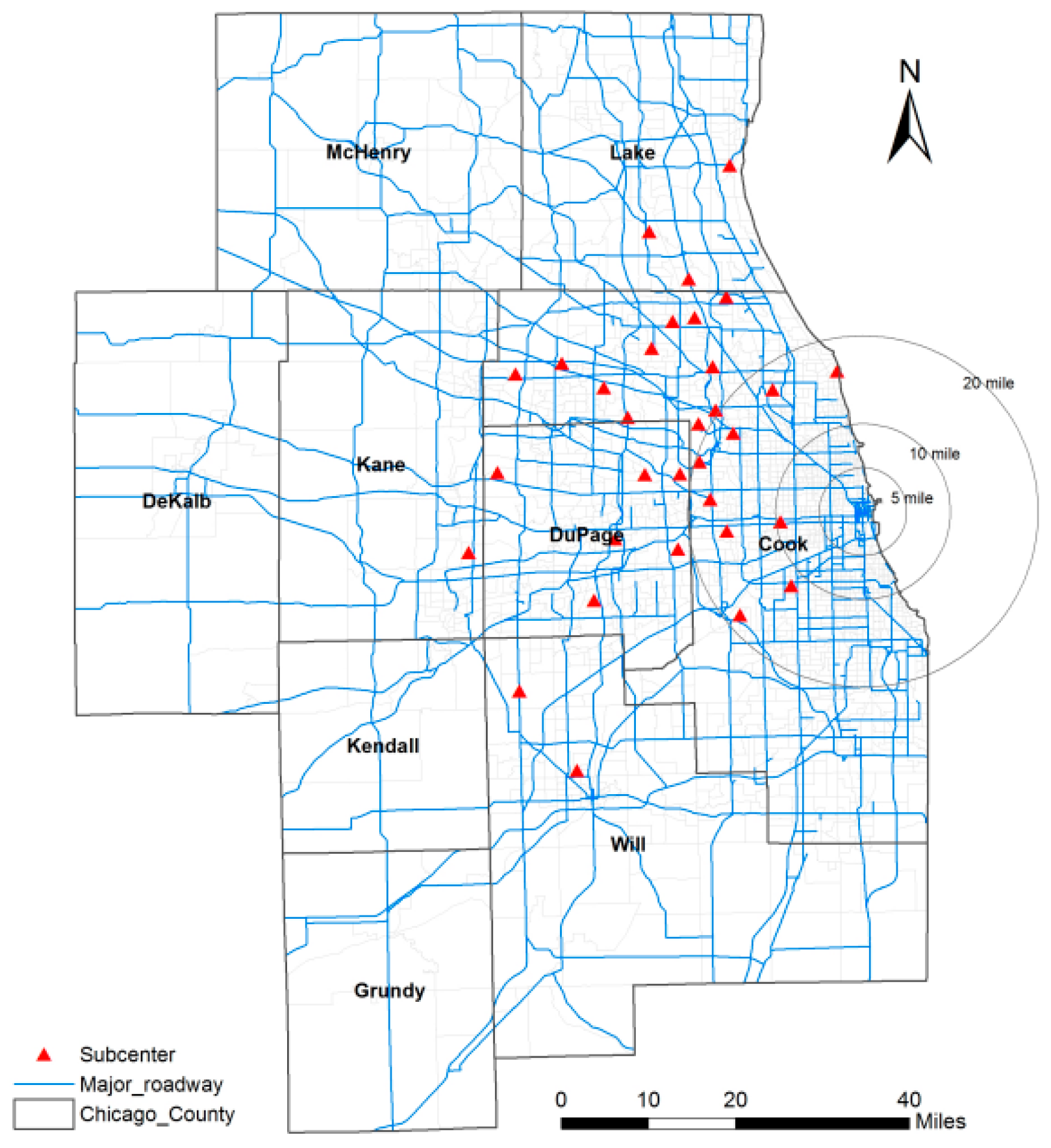
One might worry about the condition of exclusion restriction, because the distance to employment subcenter and major roadways may affect housing prices. However, these two variables do not affect housing prices directly. Specifically, unlike interstate highways or national highways, major roadways are spatially dispersed in the Chicago metropolitan region as shown in Figure 2, thus, everyone can easily access the major roadways. This is supported by the fact that the average distance from each neighborhood to the nearest major roadway is less than 0.5 miles (see Table 1). Therefore, housing prices would not be spatially sorted by the major roadways. Likewise, distance to employment subcenter is not directly related to housing prices because the simple geographical distance to the employment center does not guarantee higher property values.
4.2.4. Control Variables
Additional control variables that may affect the housing prices are included. Such variables are chosen with consideration of housing characteristics, socioeconomic characteristics, and geographical characteristics. The number of bedrooms and the average building age are used as housing characteristics. Higher number of bedrooms is expected to be associated with higher housing prices, and higher average building age is expected to be negatively associated housing prices. For socioeconomic characteristics, we include five variables. We expect that higher housing costs will be related to higher housing prices. In order to capture the effect of average age of households and size of housings in the neighborhood, we include the average age of households and household size. The proportion of African-American and Hispanic households is included to examine racial segregation in the neighborhoods. In order to capture geographical characteristics of the neighborhoods, we use residential density, the proportion of single-family housing units, distance to park, and Cook County dummy variables. Particularly, we include Cook County as a dummy variable because it includes Chicago downtown and large subcenters related to economic activities, and thus relatively higher housing prices are expected in the area.
5. Empirical Results
5.1. Descriptive Statistics
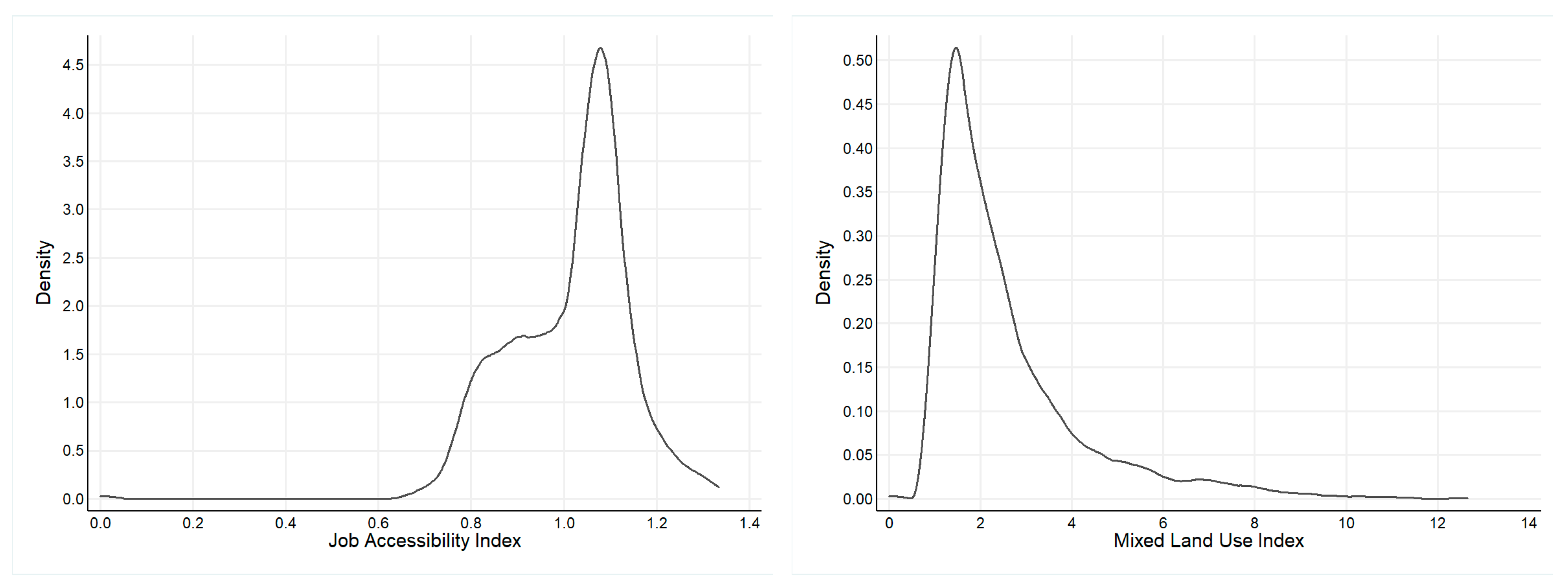
Table 1 presents the descriptive statistics of variables used in this study. Based on the ACS 2009–2013, the median housing price and median rent in the Chicago metropolitan area are $266,371 and $912, respectively. The average values of job accessibility and mixed land use are 1.01 and 2.57, respectively. Figure 3 presents a Kernel distribution of job accessibility and mixed land use, which shows that they have different distributions. Average room is 2.64, and average year built is 61. Average housing cost is $1368. Average age and average household size are 36 and 2.66, respectively. The proportions of black and Hispanic are about 20%. Average residential density is 7.25 (housing/mile2), and the proportion of single housing is about 50%. The average distance to nearest park is 0.38 miles (615 meter), and the average vacancy rate is 10%. As discussed above, our unit of analysis is census tract, and 2014 census tracts are used in this study.
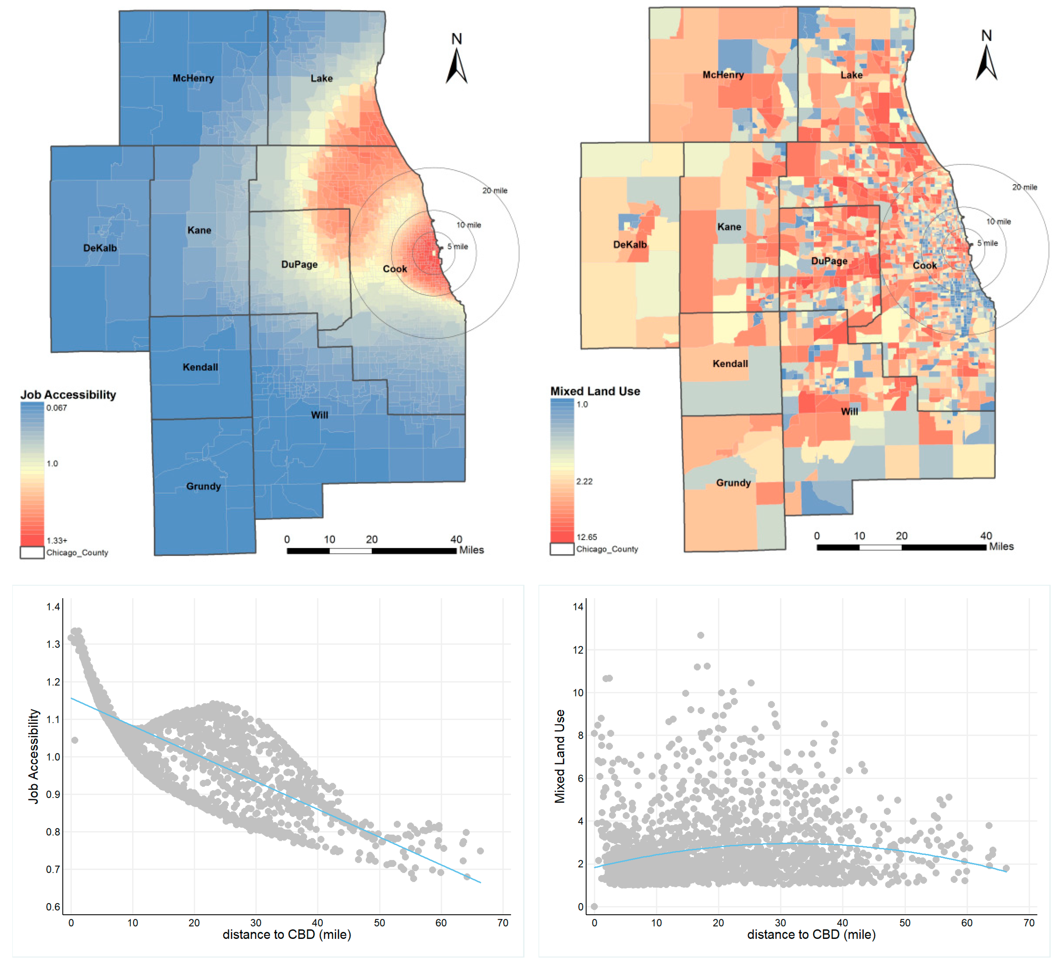
Figure 4 presents the spatial distribution of job accessibility measured based on Equation (8) and mixed land use measured based on Equation (10). Job accessibility decreases as distance from the CBD increases, but interestingly job accessibility in the northern part from the CBD is high. Although many reasons may affect this spatial distribution of job accessibility, this can be simply explained that job supply is higher than job demand. This pattern of job accessibility seems to be related to the spatial distribution of housing prices as shown in Figure 1. The mixed land use pattern looks different from the job accessibility pattern, and thus it is expected that the influence of mixed land use and job accessibility may play a different role in explaining housing prices or rents.
5.2. Empirical Results
Table 2 provides the estimated coefficients of our empirical models. As discussed above, in order to deal with endogeneity and spatial autocorrelation together, we apply GS2SLS estimator with instrumental variables. To verify the validity of instrumental variables, Hansen’s over-identification test with the null hypothesis that the instrumental variables are orthogonal to the regression error is conducted. As shown in the bottom of Table 2, the null hypothesis cannot be rejected, meaning that the instrumental variables used in this analysis are associated with land use characteristics such as job accessibility and mixed land use but are not related to the error terms. Therefore, the estimation results are reliable. The R-squares of the first-stage regression are 64% and 16%, respectively, which is provided in Appendix A.
In addition to the instrumental variables, Moran’ I as well as the estimation results of both spatial lag terms () and error terms () are statistically significant at the 1% level. This indicates that both the median housing price and rent in a neighborhood are affected by median housing price and rent in surrounding neighborhoods and are also affected by unobserved neighboring factors. Particularly, the positive signs present that an increase in housing price and rent as well as unobserved factors in neighboring census tracts lead to an increase in a housing price and rent in a given census tract. These statistical results of instrumental variables and spatial variables support the necessity of using the GS2SLS estimator in this analysis. In order to compare the results of our models (GS2SLS) that deal with spatial autocorrelation and endogeneity with the results of models (SAC) that only deal with spatial autocorrelation, we provide the results from SAC models in Appendix B.
5.2.1. Estimation Results of Median Housing Price Model
As shown in model 1 and 2 in Table 2, our key variables (job accessibility and mixed land use) are significantly associated with median housing prices, meaning that housing demanders’ preferences of the land use characteristics are reflected in the housing prices. Interestingly, the directions of the effects are different. Specifically, an increase in job accessibility causes an increase in housing price, whereas an increase in mixed land use causes a decrease in housing price. The results suggest that housing consumers are likely to pay more for the neighborhood with higher job accessibility, but they are not willing to pay for the neighborhood with higher mixed land use. Specifically, a one increase in job accessibility leads to a 1.5 percentage increase in housing prices, but a one increase in mixed land use index leads to a 0.14 percentage decrease in housing prices. These results are consistent with the evidence of previous studies that higher job accessibility increases housing values [32]. Our control variables show the expected results. For example, higher building ages, higher proportion of African-Americans, and higher proportion of single-family housing are negatively associated with housing prices. Surprisingly, the variable of single-family housing has a negative effect on housing prices. This may be because areas with higher proportions of single-family housing are located in suburbs where the housing prices are relatively lower. In contrast, the variables of average age, household size, and housing density are positively associated with housing prices. Dummy variable of Cook County is positively associated with housing prices, probably because the census tracts in Cook County are closer to downtown; furthermore, Cook County includes census tracts with a greater number of economic activities.
5.2.2. Estimation Results of Median Rent Price Model
Generally, housing markets and rental housing markets have different characteristics with respect to the demand, and the demand varies by age, income, and characteristics of households. Hence, it is expected that consumers of housing and rental housing have different preferences for land use. The results of models 3 and 4 are interesting. While job accessibility is not statistically associated with rent, mixed land use is statistically and positively associated with rent, indicating that higher index of mixed land use increases rental prices. This result implies that renters are willing to pay more for mixed land use. Specifically, one unit increase in mixed land use index leads to an increase in housing prices of 0.13 percentage. The effects of job accessibility and mixed land use on rent are different from those on housing prices, which suggests that housing consumers have different preferences compared to renters with respect to neighborhood land use characteristics.
We also briefly summarize the results of our control variables. The coefficients of year built and the proportion of single-family housing are negatively associated with median rents. This may be because census tracts with a higher proportion of single-family housing generally locate suburban areas where prices of rental housing and apartments are relatively lower. The variables of average age and household size are positively associated with rents. Finally, as expected, an increase in vacancy rates leads to a decrease in rents.
6. Conclusions and Discussion
Since land use planning is closely related to urban spatial structure and the housing market, more appropriate and effective policies are necessary to make our communities better. Although it is argued that job accessibility and mixed land use are essential elements in land use planning, evaluations of their effects have not been comprehensive; most studies have been conducted based on a supply-oriented perspective, and only a few studies have focused on housing consumers’ demand for neighborhood land use characteristics. Therefore, our understanding of which land use features meet renters’ and housing buyers’ preferences is limited. In order to fill the void, we explored consumers’ demand for land use types by examining how job accessibility and mixed land use affect housing prices and rent prices. Particularly, we employed a spatial two-stage least square model with instrumental variables to account for the endogeneity occurring between land use and housing prices, as well as spatial autocorrelation between housing prices.
Interestingly, our findings clearly demonstrated that job accessibility and mixed land use have different effects on housing prices and rents at least in the Chicago metropolitan area. For example, while job accessibility positively affects housing prices, it is not associated with rent prices. By contrast, mixed land use is negatively associated with housing prices, whereas it increases rent prices. The results indicate that housing demanders and renters have different preferences with respect to the neighborhood land use types. Specifically, housing demanders are likely to pay more prices for houses in the neighborhood with good accessibility. On the other hand, renters are willing to pay more for houses in neighborhoods with higher mixed land use.
In general, housing consumers are more likely to live in single-family neighborhoods that provide a better living environment (e.g., less noise, less air pollution, and better education services) because they earn relatively higher incomes than renters and thus can buy single-family housing [21]. In addition, they prefer neighborhoods with good job accessibility because most of them may have a car and use it for commuting. In contrast, renters are not likely to relocate to neighborhoods with higher job accessibility, but they are willing to pay for housing in areas with higher mixed land use because they prefer to live close to areas providing various services because of lower commuting costs, shorter shopping trips, and good accessibility to retail. Previous studies have shown that lower rates of home ownership are mostly due to lower incomes, lower wealth, and younger age [43]. Also, the homeownership gap can be larger between racial and ethnic groups [44]. One of the problems raised by scholars is that lower job accessibility may produce negative economic consequences such as higher unemployment rates and lower household incomes [34]. To reduce these unintended consequences, these two land use features that increase access to jobs should be encouraged in planning practice.
However, as our findings have demonstrated, mixed land use development does not meet the housing consumers’ preferences, at least in the Chicago metropolitan area, which calls into question the contemporary smart growth policies arguing that consumers value greater walking accessibility. Planning and policies should reflect the heterogeneity of the preferences between the housing demanders and renters. That is, land use practices for smart growth consider preferences of renters who have lower incomes, and minorities and housing buyers. Although this study does not examine the different preferences of housing demanders, our results suggest that there are differences between demanders’ preferences. Further analysis combined with residential location choice theory could be used to ascertain the differences.
Our findings suggest important policy implications. First, land use policy should be carefully implemented with consideration of different demanders’ different preferences. Although mixed land use development has been conducted, there are supply-oriented and comprehensive evaluations that have not been followed. More studies are necessary to understand who prefers and who does not prefer mixed land use. Second, policies for increasing job accessibility via the spatial integration of jobs and housing are necessary. Although there is no simple way to achieve it, utilizing spatial distribution of employment subcenter can be an alternative way. Particularly, functional differentiation and integration of employment subcenters would be helpful to provide a better job accessibility at the metropolitan level. However, more studies examining the relationship between the spatial distribution of the employment subcenter and housing prices are necessary. Third, the housing markets consist of different submarkets [9]. People react in the submarkets based on their different preferences. As shown in our results, land use features can differently affect housing and rental markets. City planners and land use policy makers should consider that more appropriate land use policies are necessary for meeting different needs between renters and housing demanders.
There are several limitations in our research. We use only one job accessibility and one mixed land use index, but these indices can be developed in a variety of ways. Particularly, by categorizing employment sectors, they can be developed for measuring retail-oriented, service-oriented, education-oriented, or other types-oriented job accessibility and mixed land use [4]. With these various indices, therefore, we can figure out which types of job accessibility or mixed land use are much more important for housing markets and housing demanders. More in-depth quantitative analysis should be followed, and future work should continuously investigate the relationship between land use and housing prices with consideration of the heterogeneous housing market. In addition, we suggest that disaggregate data such as individual housing prices and rents would be helpful to obtain a better understanding of the effects of land use on housing prices. Additionally, we acknowledge that we cannot control for all the endogenous variables related to housing prices through our models. For more precise estimation on the relationship between land use and housing prices, advanced econometric techniques with additional variables should be developed and applied in future research.
Author Contributions
D.K. contributed to the research design and data analysis. J.J. contributed to the writing and supervised the research. D.K. and J.J. put forward the concept of this article, led the development of methodology, and helped with the modifying of the manuscript. All authors contributed to the writing, reviewing, and correction in this manuscript.
Funding
This work was supported by a grant from Kyung Hee University in 2017, grant number [KHU-20171751].
Acknowledgments
This research was funded by a grant [KHU-20171751] through the Kyung Hee University.
Conflicts of Interest
The authors declare no conflict of interest.
Appendix A

Table A1.
Estimation Results of the First-Stage Regression
| Accessibility | Mixed Land Use | |
|---|---|---|
| Subcenters | −0.0077 *** | −0.0200 * |
| (0.0004) | (0.0078) | |
| Major Roadways | −0.0291 *** | −0.6192 *** |
| (0.0047) | (0.0909) | |
| Bedrooms | 0.0202 ** | −0.5039 *** |
| (0.0092) | (0.1788) | |
| Year Built | 0.0001 *** | −0.0003 |
| (0.0000) | (0.0002) | |
| Housing Cost | 0.0001 *** | 0.0005 *** |
| (0.0000) | (0.0001) | |
| % Single-Family Housing | −0.2020 *** | −0.2450 |
| (0.0118) | (0.2284) | |
| % Black | 0.0065 | −0.9204 *** |
| (0.0087) | (0.1685) | |
| % Hispanic | 0.0588 *** | −0.2603 |
| (0.0135) | (0.2620) | |
| Average Age | 0.0031 *** | 0.0402 *** |
| (0.0004) | (0.0069) | |
| Household Size | −0.0021 | −0.0709 |
| (0.0078) | (0.1508) | |
| Housing Density | 0.0007 *** | −0.0177 *** |
| (0.0001) | (0.0024) | |
| Distance to Park | 0.0000 *** | 0.0001 *** |
| (0.0000) | (0.0000) | |
| Vacant Rate | 0.1762 *** | 0.8931 |
| (0.0307) | (0.5953) | |
| Cook County | 0.0904 *** | −0.3975 *** |
| (0.0046) | (0.0885) | |
| Constant | 0.8151 *** | 2.9839 *** |
| (0.0194) | (0.3763) | |
| N | 2014 | 2014 |
| R2 | 0.6413 | 0.1616 |
Note: ***, **, and * indicate significance at the 0.1%, 1%, and 5% levels, respectively; std. errors are in parentheses.
Appendix B
Table A2.
Estimation Results of SAC models
| Housing Price | Rent Price | |
|---|---|---|
| Job Accessibility | 4.7407 *** | 1.0541 |
| (0.4181) | (0.6442) | |
| Mixed Land Use | 0.0196 | 0.0347 *** |
| (0.0129) | (0.0153) | |
| Bedrooms | −0.0723 | −0.1631 |
| (0.1128) | (0.1336) | |
| Year Built | −0.0014 *** | −0.0009 *** |
| (0.0001) | (0.0002) | |
| Housing Cost | 0.0006 *** | 0.0002 *** |
| (0.0001) | (0.0001) | |
| % Single-Family Housing | −0.4029 ** | −0.3237 * |
| (0.1622) | (0.1904) | |
| % Black | −0.3814 ** | 0.0548 |
| (0.1562) | (0.1729) | |
| % Hispanic | 0.1409 | 0.2441 |
| (0.2085) | (0.2388) | |
| Average Age | 0.0599 *** | 0.0197 *** |
| (0.0046) | (0.0053) | |
| Household Size | 0.5820 *** | 0.1984 * |
| (0.0983) | (0.1136) | |
| Housing Density | 0.0006 | −0.0001 |
| (0.0014) | (0.0016) | |
| Distance to Park | 0.0001 | 0.0001 |
| (0.0000) | (0.0000) | |
| Vacant Rate | −0.4784 | 0.6003 |
| (0.3458) | (0.4109) | |
| Cook County | −0.2303 | −0.3190 |
| (0.1209) | (0.2282) | |
| Constant | 8.4991 *** | 6.8423 *** |
| (0.7412) | (0.5565) | |
| 0.4008 *** | 0.3431 *** | |
| (0.0559) | (0.0709) | |
| 0.3167 *** | 0.2437 *** | |
| (0.0319) | (0.0419) | |
| N | 2014 | 2014 |
| Log-Likelihood | −2606.47 | −2967.31 |
| Moran’s I | 0.4379 *** | 0.3743 *** |
Note: ***, **, and * indicate significance at the 0.1%, 1%, and 5% levels, respectively; std. errors are in parentheses.
References
- Ewing, R.; Cervero, R. Travel and the built environment: A meta-analysis. J. Am. Plann. Assoc. 2010, 76, 265–294. [Google Scholar] [CrossRef]
- Jacobs, J. The Death and Life of Great American Cities, 1st ed.; A Division of Random House: New York, NY, USA, 1961. [Google Scholar]
- Shen, Q. Location characteristics of inner-city neighborhoods and employment accessibility of low-wage workers. Environ. Plan. B. 1998, 25, 345–365. [Google Scholar] [CrossRef]
- Hu, L. Changing job access of the poor: Effects of spatial and socioeconomic transformations in Chicago, 1990–2010. Urban Stud. 2013, 51, 675–692. [Google Scholar] [CrossRef]
- Guo, J.; Bhat, C. Operationalizing the concept of neighborhood: Application to residential location choice analysis. J. Transp. Geogr. 2007, 15, 31–45. [Google Scholar] [CrossRef]
- Cervero, R.; Duncan, M. Which reduces vehicle travel more: Jobs-housing balance or retail-housing mixing? J. Am. Plann. Assoc. 2006, 72, 475–490. [Google Scholar] [CrossRef]
- Schimer, P.; van Eggermond, M.; Axhausen, K. The role of location in residential location choice models: A review of literature. J. Transp. Land Use. 2014, 7, 3–21. [Google Scholar] [CrossRef]
- Jin, J.; Lee, H. Understanding residential location choices: An application of the UrbanSim residential location model on Suwon, Korea. Int. J. Urban Sci. 2018, 22, 216–235. [Google Scholar] [CrossRef]
- Boeing, G.; Waddell, P. New insights into rental housing markets across the United State: Web scraping and analyzing Craiglist rental listings. J. Plan. Edu. Res. 2017, 37, 457–476. [Google Scholar] [CrossRef]
- Koster, H.; Rouwendal, J. The impact of mixed land use on residential property values. J. Reg. Sci. 2012, 52, 733–761. [Google Scholar] [CrossRef]
- Plaut, P.; Boarnet, M. New urbanism and the value of neighborhood design. J. Archit. Plan. Res. 2003, 20, 254–265. [Google Scholar]
- Kitamura, R.; Mokhtarian, P.; Laidet, L. A micro-analysis of land use and travel in five neighborhoods in the San Francisco Bay Area. Transportation 1997, 24, 125–158. [Google Scholar] [CrossRef]
- Painter, G.; Gabriel, S.; Myers, D. Race, immigrant status, and housing tenure choice. J. Urban Econ. 2001, 49, 150–167. [Google Scholar] [CrossRef]
- Song, Y.; Knaap, G. Measuring the effects of mixed land uses on housing values. Reg. Sci. Urban Econ. 2004, 34, 663–680. [Google Scholar] [CrossRef]
- Ewing, R.; Cervero, R. Travel and the built environment: A Synthesis. Transp. Res. Rec. 2001, 1780, 87–114. [Google Scholar] [CrossRef]
- Crane, R. The influence of urban form on travel: An interpretive review. J. Plan. Lit. 2000, 15, 3–23. [Google Scholar] [CrossRef]
- Frank, L.; Pivo, G. Impact of mixed use and density on utilization of three modes of travel: Single-Occupant vehicle, transit, and walking. Transp. Res. Rec. 1994, 44–52. [Google Scholar]
- Rosen, S. Hedonic prices and implicit markets: Product differentiation in pure competition. J. Political. Econ. 1974, 82, 34–55. [Google Scholar] [CrossRef]
- Gibbons, S.; Machin, S. Valuing rail access using transport innovations. J. Urban Econ. 2005, 57, 148–169. [Google Scholar] [CrossRef] [Green Version]
- Armstrong, R.; Rodriguez, D. An evaluation of the accessibility benefits of commuter rail in Eastern Massachusetts using spatial hedonic price functions. Transportation 2006, 33, 21–43. [Google Scholar] [CrossRef]
- Cervero, R.; Duncan, M. Neighborhood composition and residential land prices: Does exclusion raise or lower values? Urban Stud. 2004, 41, 299–315. [Google Scholar] [CrossRef]
- Matthews, J.; Turnbull, G. Neighborhood street layout and property values: the interaction of accessibility and land use mix. J. R. Estate Finance Econ. 2007, 35, 111–141. [Google Scholar] [CrossRef]
- Alonso, W. Location and Land Use; Harvard University Press: Cambridge, MA, USA, 1964. [Google Scholar]
- Muth, R. Cities and Housing: The Spatial Pattern of Urban Residential Land Use; University of Chicago Press: Chicago, IL, USA, 1969. [Google Scholar]
- Mills, E. Markets and efficient resource allocation in urban areas. Swed. J. Econ. 1972, 74, 100–113. [Google Scholar] [CrossRef]
- Anas, A.; Richard, A.; Small, K. Urban spatial structure. J. Econ. Lit. 1998, 36, 1426–1464. [Google Scholar]
- Giuliano, G.; Small, K. Subcenters in the Los Angeles region. Reg. Sci. Urban Econ. 1991, 21, 163–182. [Google Scholar] [CrossRef]
- McMillen, D. Nonparametric employment subcenter identification. J. Urban Econ. 2001, 50, 448–473. [Google Scholar] [CrossRef]
- Hansen, W. How accessibility shapes land use. J. Am. Inst. Plan. 1959, 25, 73–76. [Google Scholar] [CrossRef]
- Noland, C. Assessing hedonic indexes for housing. J. Finan. Quant. Anal. 1979, 14, 783–800. [Google Scholar] [CrossRef]
- Waddell, P. UrbanSim: Modeling urban development for land use, transportation, and environmental planning. J. Am. Plann. Assoc. 2002, 68, 297–314. [Google Scholar] [CrossRef]
- Osland, L.; Thorsen, I. Effects on housing prices of urban attraction and labor-market accessibility. Environ. Plan. A 2008, 40, 2490–2509. [Google Scholar] [CrossRef]
- Cervero, R.; Rood, T.; Appleyard, B. Tracking accessibility: Employment and housing opportunities in the San Francisco Bay Area. Environ. Plan. A 1999, 31, 1259–1278. [Google Scholar] [CrossRef]
- Jin, J.; Paulsen, K. Does accessibility matter? Understanding the effect of job accessibility on labor market outcomes. Urban Stud. 2018, 55, 91–115. [Google Scholar]
- Cao, T.; Cory, D. Mixed land uses, land-use externalities, and residential property values: A reevaluation. Ann. Regional Sci. 1982, 16, 1–24. [Google Scholar]
- Song, Y.; Knaap, G. New urbanism and housing values: A disaggregate assessment. J. Urban Econ. 2003, 54, 218–238. [Google Scholar] [CrossRef]
- Aurand, A. Density, housing types and mixed land use: Smart tools for affordable housing? Urban Stud. 2010, 47, 1015–1036. [Google Scholar] [CrossRef]
- Malpezzi, S. Hedonic pricing model: A selective and applied review. In Housing Economics and Public Policy; O’Sullivan, T., Gibb, K., Eds.; Blackwell Science: Oxford, UK, 2003. [Google Scholar]
- Anselin, L. Lagrange multiplier test diagnostics for spatial dependence and spatial heterogeneity. Geogr. Anal. 1988, 20, 1–17. [Google Scholar] [CrossRef]
- Duranton, G.; Puga, D. Diversity and specialization in cities: Why, where and when does it matter? Urban Stud. 2000, 37, 533–555. [Google Scholar] [CrossRef]
- McMillen, D.; McDonald, J. Suburban subcenters and employment density in metropolitan Chicago. J. Urban Econ. 1998, 43, 157–180. [Google Scholar] [CrossRef]
- McMillen, D. Employment subcenters in Chicago: Past, present, and future. J. Econ. Perspect. 2003, 2Q, 2–14. [Google Scholar]
- Gyourko, J.; Linneman, P. An analysis of the changing influences on traditional household ownership patterns. J. Urban Econ. 1996, 39, 318–341. [Google Scholar] [CrossRef]
- Levine, J.; Inam, A.; Torng, G. A Choce-based rationale for land use and transportation alternatives: Evidence from Boston and Atlanta. J. Plan. Educ. Res. 2005, 24, 317–330. [Google Scholar] [CrossRef]
Figure 1.
Spatial Distribution of the Housing Price (a) and Rent (b) (Median Values: $).

Figure 2.
Spatial Distribution of Subcenters and Major Roadways in Chicago.

Figure 3.
Density of Job Accessibility Index and Mixed Land Use.

Figure 4.
Spatial Distribution of Job Accessibility and Mixed Land Use.

Table 1.
Descriptive Statistics and Data Source.
| Variable | Mean | S.D. | Data Source | ||
|---|---|---|---|---|---|
| Dependent | Median Housing Price | 266,371.02 | 137,715.70 | ACS 2009–2013 | |
| Median Rent | 912.06 | 347.67 | ACS 2009–2013 | ||
| Independent | Land Use | Job Accessibility | 1.01 | 0.13 | LEHD LODES |
| Mixed Land Use | 2.57 | 1.66 | LEHD LODES | ||
| Control | Housing | Bedrooms | 2.64 | 0.57 | ACS 2009–2013 |
| Built Year | 61.68 | 145.90 | ACS 2009–2013 | ||
| Socioeconomic | Housing Costs | 1368.28 | 500.72 | ACS 2009–2013 | |
| Average Age | 36.21 | 7.01 | ACS 2009–2013 | ||
| Household Size | 2.66 | 0.54 | ACS 2009–2013 | ||
| % Black | 0.21 | 0.33 | ACS 2009–2013 | ||
| % Hispanic | 0.21 | 0.24 | ACS 2009–2013 | ||
| Geographic | Residential Density | 7.25 | 16.14 | ACS 2009–2013 | |
| % Single Housing | 0.50 | 0.31 | ACS 2009–2013 | ||
| Distance to Park (m) | 615.98 | 909.91 | Info USA | ||
| Vacancy Rate | 0.10 | 0.08 | ACS 2009–2013 | ||
| Dummy variable (Cook County) | 0.65 | 0.48 | 2013 Tiger/Line Shapefiles | ||
| Instrument | Distance to main road | 0.47 | 0.41 | NHS | |
| Distance to subcenters | 6.12 | 5.18 | McMillen, 2003 |
Table 2.
Estimation Results on the Effects of Job Accessibility and Mixed Land Use.
| Housing Price | Rent | |||
|---|---|---|---|---|
| GS2SLS (1) | GS2SLS (2) | GS2SLS (3) | GS2SLS (4) | |
| Job Accessibility | 1.5406 *** | 0.3853 | ||
| (0.3508) | (0.3332) | |||
| Mixed Land Use | −0.1479 *** | 0.1273 ** | ||
| (0.0502) | (0.0528) | |||
| Bedrooms | 0.0446 | 0.1171 | 0.2333 * | 0.1706 |
| (0.1114) | (0.1184) | (0.1209) | (0.1289) | |
| Year Built | −0.0016 *** | −0.0015 *** | −0.0009 *** | −0.0009 *** |
| (0.0001) | (0.0002) | (0.0002) | (0.0002) | |
| Housing Cost | 0.0007 *** | 0.0008 *** | 0.0003 *** | 0.0003 *** |
| (0.0001) | (0.0001) | (0.0001) | (0.0001) | |
| % Single-Family Housing | −0.7218 *** | −1.1379 *** | −0.3277 * | −0.4057 *** |
| (0.1636) | (0.1524) | (0.1683) | (0.1560) | |
| % Black | −0.1034 | −0.2347 * | 0.0302 | 0.1397 |
| (0.1176) | (0.1274) | (0.1042) | (0.1233) | |
| % Hispanic | 0.1947 | 0.2330 | 0.1846 | 0.2359 |
| (0.1726) | (0.1758) | (0.1659) | (0.1794) | |
| Average Age | 0.0689 *** | 0.0804 *** | 0.0292 *** | 0.0263 *** |
| (0.0044) | (0.0049) | (0.0047) | (0.0053) | |
| Household Size | 0.6714 *** | 0.7125 *** | 0.2421 ** | 0.2667 *** |
| (0.0933) | (0.0957) | (0.0957) | (0.1018) | |
| Housing Density | 0.0036 ** | 0.0021 * | −0.0002 | 0.0024 |
| (0.0015) | (0.0013) | (0.0016) | (0.0019) | |
| Distance to Park | 0.0001 | 0.0001 | 0.0001 | 0.0001 |
| (0.0000) | (0.0000) | (0.0000) | (0.0000) | |
| Vacant Rate | −0.2463 | −0.0156 | −0.7766 * | |
| (0.3659) | (0.3810) | −0.8107 **) | (0.4134) | |
| Cook County | 0.1436 ** | 0.1505 ** | −0.0307 | 0.0522 |
| (0.0728) | (0.0647) | (0.0608) | (0.0632) | |
| Constant | 3.2049 *** | 4.3759 *** | 2.8919 *** | 3.4592 *** |
| (0.7297) | (0.7268) | (0.8665) | (0.9488) | |
| 0.2325 *** | 0.2602 *** | 0.2920 ** | 0.1884 *** | |
| (0.0558) | (0.0572) | (0.1313) | (0.0429) | |
| 0.2057 *** | 0.1434 ** | 0.2073 ** | 0.1642 ** | |
| (0.0566) | (0.0589) | (0.1190) | (0.0541) | |
| N | 2014 | 2014 | 2014 | 2014 |
| Wald chi2 | 641.49 *** | 115.88 *** | 648.9 *** | 126.6 *** |
| Hansen’s Over-identification Test | 0.7037 | 1.2791 | 2.5996 | 2.6109 |
| First-Stage R2 | 0.6413 | 0.6413 | 0.1616 | 0.1616 |
| Moran’s I | 0.4379 *** | 0.4379 *** | 0.3743 *** | 0.3743 *** |
Note: ***, **, and * indicate significance at the 0.1%, 1%, and 5% levels, respectively; std. errors are in parentheses.
© 2019 by the authors. Licensee MDPI, Basel, Switzerland. This article is an open access article distributed under the terms and conditions of the Creative Commons Attribution (CC BY) license (http://creativecommons.org/licenses/by/4.0/).
Share and Cite
MDPI and ACS Style
Kim, D.; Jin, J. The Effect of Land Use on Housing Price and Rent: Empirical Evidence of Job Accessibility and Mixed Land Use. Sustainability 2019, 11, 938. https://0-doi-org.brum.beds.ac.uk/10.3390/su11030938
AMA Style
Kim D, Jin J. The Effect of Land Use on Housing Price and Rent: Empirical Evidence of Job Accessibility and Mixed Land Use. Sustainability. 2019; 11(3):938. https://0-doi-org.brum.beds.ac.uk/10.3390/su11030938
Chicago/Turabian StyleKim, Danya, and Jangik Jin. 2019. "The Effect of Land Use on Housing Price and Rent: Empirical Evidence of Job Accessibility and Mixed Land Use" Sustainability 11, no. 3: 938. https://0-doi-org.brum.beds.ac.uk/10.3390/su11030938
Note that from the first issue of 2016, this journal uses article numbers instead of page numbers. See further details here.