Application of SWAT Model with a Modified Groundwater Module to the Semi-Arid Hailiutu River Catchment, Northwest China


Abstract
:1. Introduction
2. Materials and Methods
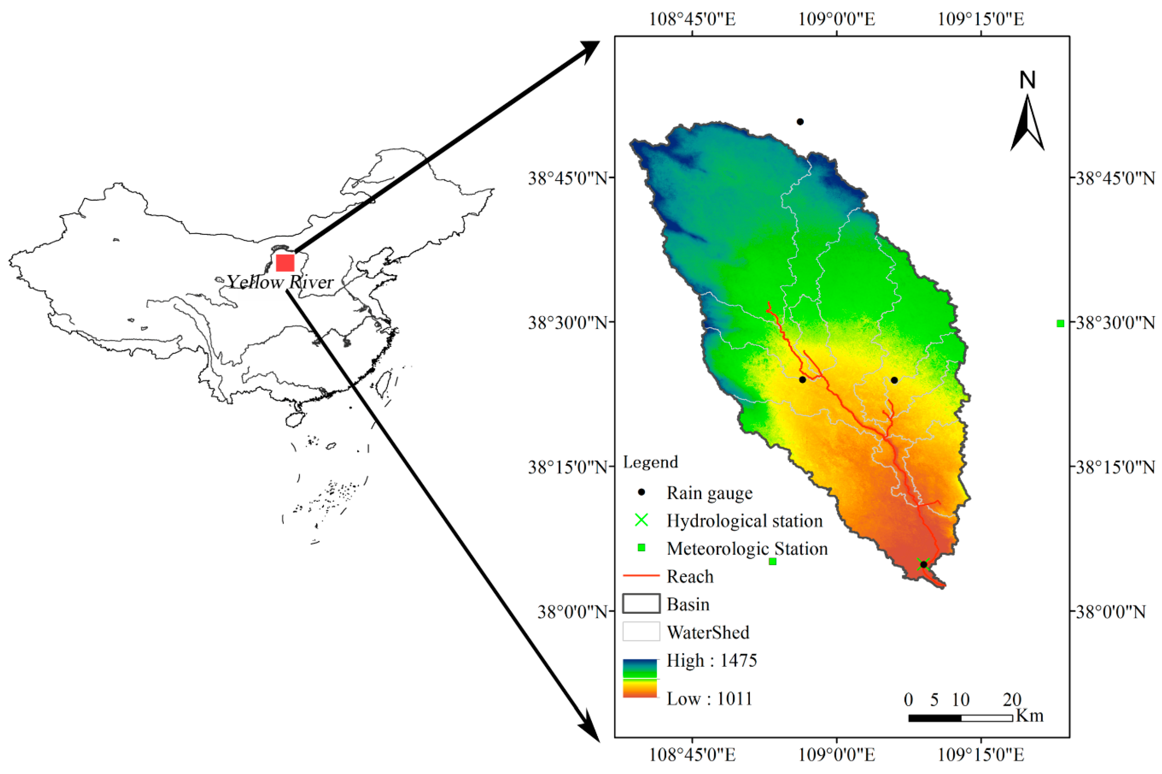
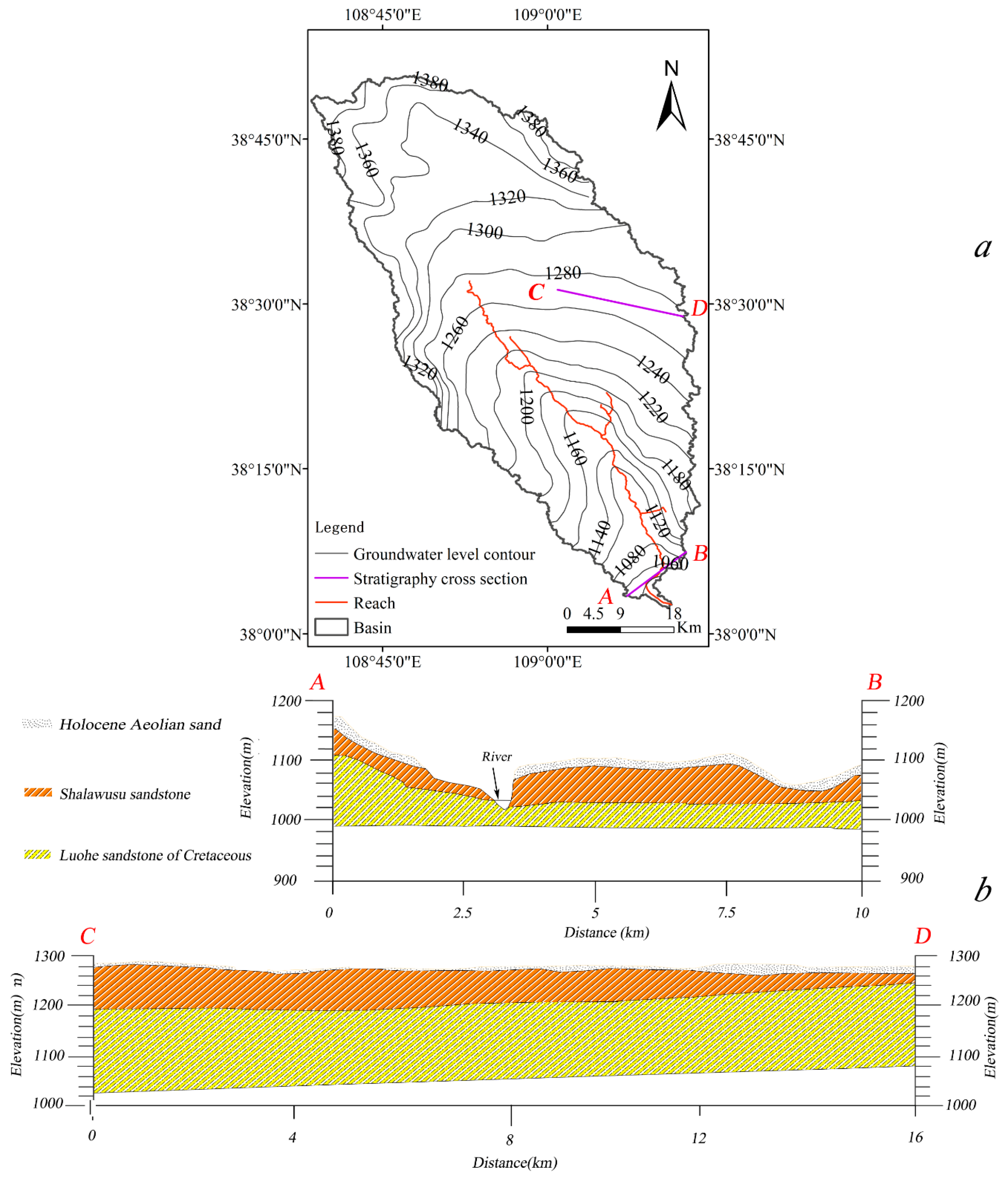
2.1. Study Area
2.2. Data Collection
2.3. Introduction of SWAT Model
2.3.1. Original SWAT Model
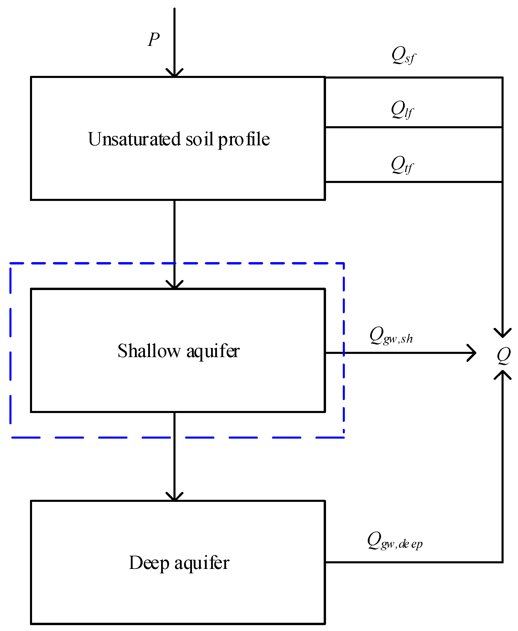
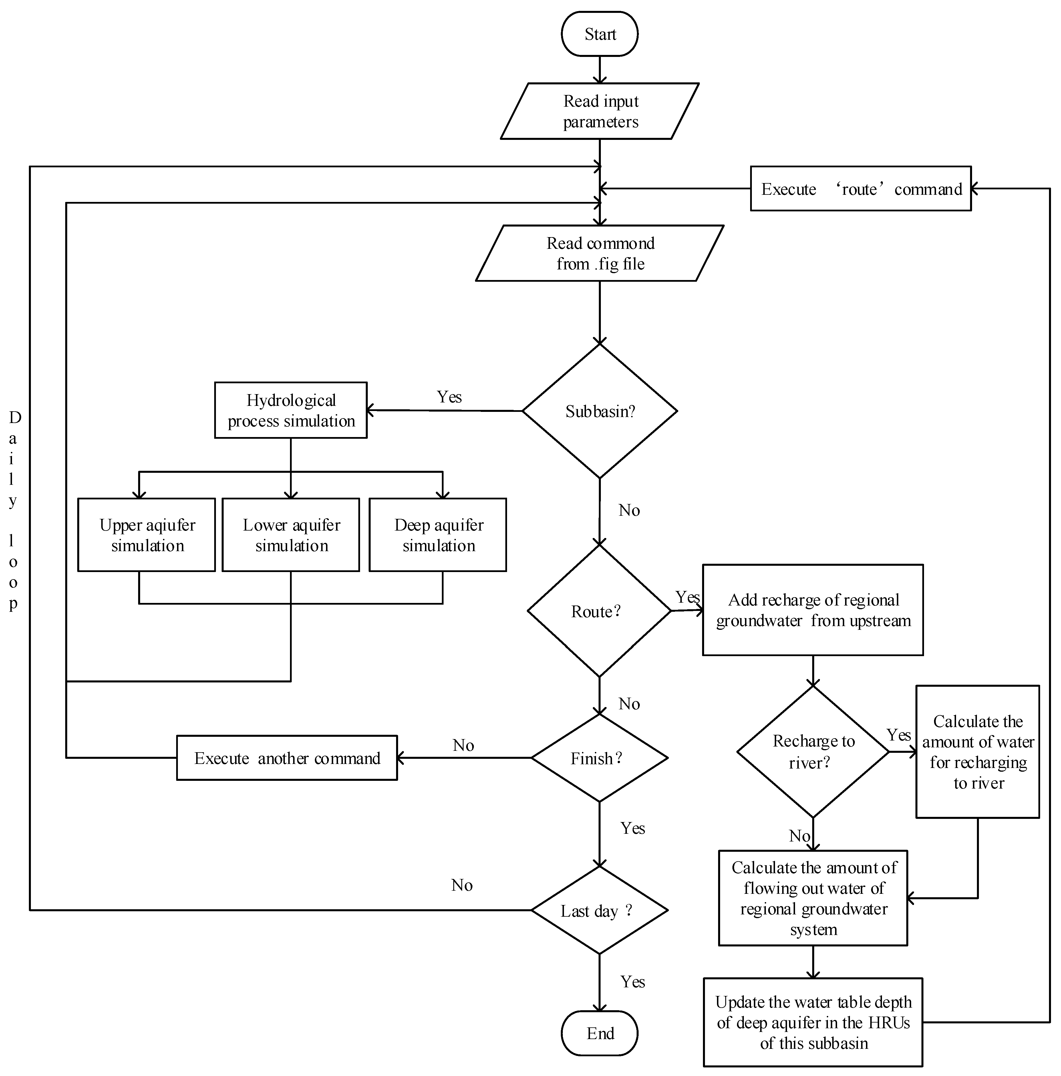
2.3.2. Modified SWAT Model
2.4. Evaluation Criteria
3. Results and Discussion
4. Conclusions
Author Contributions
Funding
Acknowledgments
Conflicts of Interest
References
- Shrestha, M.K.; Recknagel, F.; Frizenschaf, J.; Meyer, W. Assessing SWAT models based on single and multi-site calibration for the simulation of flow and nutrient loads in the semi-arid Onkaparinga catchment in South Australia. Agric. Water Manag. 2016, 175, 61–71. [Google Scholar] [CrossRef]
- Niu, J.; Phanikumar, M.S. Modeling watershed-scale solute transport using an integrated, process-based hydrologic model with applications to bacterial fate and transport. J. Hydrol. 2015, 529, 35–48. [Google Scholar] [CrossRef]
- Lu, S.; Andersen, H.E.; Thodsen, H.; Rubek, G.H.; Trolle, D. Extended SWAT model for dissolved reactive phosphorus transport in tile-drained fields and catchments. Agric. Water Manag. 2016, 175, 78–90. [Google Scholar] [CrossRef]
- Liu, R.; Xu, F.; Zhang, P.; Yu, W.; Men, C. Identifying non-point source critical source areas based on multi-factors at a basin scale with SWAT. J. Hydrol. 2016, 533, 379–388. [Google Scholar] [CrossRef]
- Gassman, P.W.; Reyes, M.R.; Green, C.H.; Arnold, J.G. The soil and water assessment tool: Historical development, applications, and future research directions. Trans. ASABE 2007, 50, 1211–1250. [Google Scholar] [CrossRef]
- Zhang, A.; Liu, W.; Yin, Z.; Fu, G.; Zheng, C. How Will Climate Change Affect the Water Availability in the Heihe River Basin, Northwest China? J. Hydrometeor. 2016, 17, 1517–1542. [Google Scholar] [CrossRef]
- Guo, H.; Hu, Q.; Jiang, T. Annual and seasonal streamflow responses to climate and land-cover changes in the Poyang Lake basin, China. J. Hydrol. 2008, 355, 106–122. [Google Scholar] [CrossRef]
- Guo, L.; Chen, J.; Lin, H. Subsurface lateral preferential flow network revealed by time-lapse ground-penetrating radar in a hillslope. Water Resour. Res. 2014, 50, 9127–9147. [Google Scholar] [CrossRef] [Green Version]
- Zhang, Q.; Liu, J.; Singh, V.P.; Gu, X.; Chen, X. Evaluation of impacts of climate change and human activities on streamflow in the Poyang Lake basin, China: Impacts of Climate Change and Human Activities on Streamflow. Hydrol. Process. 2016, 30, 2562–2576. [Google Scholar] [CrossRef]
- Tuppad, P.; Douglas-Mankin, K.R.; Lee, T.; Srinivasan, R.; Arnold, J.G. Soil and Water Assessment Tool (SWAT) hydrologic/water quality model: Extended capability and wider adoption. Trans. ASABE 2011, 54, 1677–1684. [Google Scholar] [CrossRef]
- Sellami, H.; Benabdallah, S.; La Jeunesse, I.; Vanclooster, M. Quantifying hydrological responses of small Mediterranean catchments under climate change projections. Sci. Total Environ. 2016, 543(Pt. B), 924–936. [Google Scholar] [CrossRef]
- Čerkasova, N.; Ertürk, A.; Zemlys, P.; Denisov, V.; Umgiesser, G. Curonian Lagoon drainage basin modelling and assessment of climate change impact. Oceanologia 2016, 58, 90–102. [Google Scholar] [CrossRef] [Green Version]
- Muttiah, R.S.; Wurbs, R.A. Modeling the impacts of climate change on water supply reliabilities. Water Int. 2002, 27, 407–419. [Google Scholar] [CrossRef]
- Gosain, A.K.; Rao, S.; Basuray, D. Climate change impact assessment on hydrology of Indian river basins. Curr. Sci. 2006, 346–353. [Google Scholar]
- Qi, J.; Li, S.; Jamieson, R.; Hebb, D.; Xing, Z.; Meng, F.-R. Modifying SWAT with an energy balance module to simulate snowmelt for maritime regions. Environ. Model. Softw. 2017, 93, 146–160. [Google Scholar] [CrossRef]
- Chen, Y.; Marek, G.W.; Marek, T.H.; Brauer, D.K.; Srinivasan, R. Improving SWAT auto-irrigation functions for simulating agricultural irrigation management using long-term lysimeter field data. Environ. Model. Softw. 2018, 99, 25–38. [Google Scholar] [CrossRef]
- Tsuchiya, R.; Kato, T.; Jeong, J.; Arnold, J.G. Development of SWAT-Paddy for Simulating Lowland Paddy Fields. Sustainability 2018, 10, 3246. [Google Scholar] [CrossRef]
- Shirmohammadi, A.; Chu, T.W. Evaluation of the swat model’s hydrology component in the piedmont physiographic region of maryland. Trans. ASAE 2004, 47, 1057–1073. [Google Scholar]
- Amatya, D.M.; Jha, M.; Edwards, A.E.; Williams, T.M.; Hitchcock, D.R. SWAT-based streamflow and embayment modeling of karst-affected Chapel branch watershed, South Carolina. Trans. ASABE 2011, 54, 1311–1323. [Google Scholar] [CrossRef]
- Cheng, L.; Xu, Z.X.; Luo, R. SWAT application in arid and semi-arid region: A case study in the Kuye River Basin. Geogr. Res. 2009, 28, 65–73. [Google Scholar]
- Pfannerstill, M.; Guse, B.; Fohrer, N. A multi-storage groundwater concept for the SWAT model to emphasize nonlinear groundwater dynamics in lowland catchments. Hydrol. Process. 2014, 28, 5599–5612. [Google Scholar] [CrossRef]
- Wu, K.; Johnston, C.A. Hydrologic response to climatic variability in a Great Lakes Watershed: A case study with the SWAT model. J. Hydrol. 2007, 337, 187–199. [Google Scholar] [CrossRef]
- Wittenberg, H. Baseflow recession and recharge as nonlinear storage processes. Hydrol. Process. 1999, 13, 715–726. [Google Scholar] [CrossRef]
- Eris, E.; Wittenberg, H. Estimation of baseflow and water transfer in karst catchments in Mediterranean Turkey by nonlinear recession analysis. J. Hydrol. 2015, 530, 500–507. [Google Scholar] [CrossRef]
- Wang, Y.; Brubaker, K. Implementing a nonlinear groundwater module in the soil and water assessment tool (SWAT). Hydrol. Process. 2014, 28, 3388–3403. [Google Scholar] [CrossRef]
- Gan, R.; Luo, Y. Using the nonlinear aquifer storage–discharge relationship to simulate the base flow of glacier- and snowmelt-dominated basins in northwest China. Hydrol. Earth Syst. Sci. 2013, 17, 3577–3586. [Google Scholar] [CrossRef] [Green Version]
- Guzman, J.A.; Moriasi, D.N.; Gowda, P.H.; Steiner, J.L.; Starks, P.J.; Arnold, J.G.; Srinivasan, R. A model integration framework for linking SWAT and MODFLOW. Environ. Model. Softw. 2015, 73, 103–116. [Google Scholar] [CrossRef]
- Kim, N.W.; Chung, I.M.; Won, Y.S.; Arnold, J.G. Development and application of the integrated SWAT–MODFLOW model. J. Hydrol. 2008, 356, 1–16. [Google Scholar] [CrossRef]
- Wei, X.; Bailey, R.T. Using SWAT-MODFLOW to simulate groundwater flow and groundwater-surface water interactions in an intensively irrigated stream-aquifer system. In Proceedings of the Agu Fall Meeting, New Orleans, LA, USA, 11–15 December 2017. [Google Scholar]
- Chu, J.; Chi, Z.; Zhou, H. Research and Application of Interface and Frame Structure of SWAT and MODFLOW Models Coupling. Prog. Geogr. 2011, 30, 335–342. [Google Scholar]
- Nguyen, V.T.; Dietrich, J. Modification of the SWAT model to simulate regional groundwater flow using a multicell aquifer. Hydrol. Process. 2018, 32, 939–953. [Google Scholar] [CrossRef]
- Yang, Z.; Zhou, Y.; Wenninger, J.; Uhlenbrook, S. A multi-method approach to quantify groundwater/surface water-interactions in the semi-arid Hailiutu River basin, northwest China. Hydrogeol. J. 2014, 22, 527–541. [Google Scholar] [CrossRef]
- Zhou, Y.; Yang, Z.; Zhang, D.; Jin, X.; Zhang, J. Inter-catchment comparison of flow regime between the Hailiutu and Huangfuchuan rivers in the semi-arid Erdos Plateau, Northwest China. Hydrol. Sci. J. 2015, 60, 688–705. [Google Scholar] [CrossRef]
- Huang, J.; Hou, G.; Li, H.; Yin, L.; Lu, H.; Zhang, J.; Dong, J. Estimating subdaily evapotranspiration rates using the corrected diurnal water-table fluctuations in a shallow groundwater table area. In Proceedings of the 2011 International Symposium on Water Resource and Environmental Protection, Xi’an China, 20–22 May 2011; Volume 4, pp. 3093–3099. [Google Scholar]
- Yin, L.; Zhou, Y.; Huang, J.; Wenninger, J.; Hou, G.; Zhang, E.; Wang, X.; Dong, J.; Zhang, J.; Uhlenbrook, S. Dynamics of willow tree (Salix matsudana) water use and its response to environmental factors in the semi-arid Hailiutu River catchment, Northwest China. Environ. Earth Sci. 2014, 71, 4997–5006. [Google Scholar] [CrossRef]
- Zhou, Y.; Wenninger, J.; Yang, Z.; Yin, L.; Huang, J.; Hou, L.; Wang, X.; Zhang, D.; Uhlenbrook, S. Groundwater–surface water interactions, vegetation dependencies and implications for water resources management in the semi-arid Hailiutu River catchment, China—A synthesis. Hydrol. Earth Syst. Sci. 2013, 17, 2435–2447. [Google Scholar] [CrossRef]
- Yin, L.; Hu, G.; Huang, J.; Wen, D.; Dong, J.; Wang, X.; Li, H. Groundwater-recharge estimation in the Ordos Plateau, China: Comparison of methods. Hydrogeol. J. 2011, 19, 1563–1575. [Google Scholar] [CrossRef]
- Wang, X.-S.; Zhou, Y. Shift of annual water balance in the Budyko space for catchments with groundwater-dependent evapotranspiration. Hydrol. Earth Syst. Sci. 2016, 20, 3673–3690. [Google Scholar] [CrossRef] [Green Version]
- Yang, Z.; Zhou, Y.; Wenninger, J.; Uhlenbrook, S. The causes of flow regime shifts in the semi-arid Hailiutu River, Northwest China. Hydrol. Earth Syst. Sci. 2012, 16, 87–103. [Google Scholar] [CrossRef] [Green Version]
- Neitsch, S.L.; Arnold, J.G.; Kiniry, J.R.; Williams, J.R. Soil and Water Assessment Tool Theoretical Documentation Version 2009; Texas Water Resources Institute: College Station, TX, USA, 2011. [Google Scholar]
- Yin, L.; Hou, G.; Jinting, H.; Ying, L.; Xiayong, W.; Zhi, Y.; Yangxiao, Z. Using chloride mass-balance and stream hydrographs to estimate groundwater recharge in the Hailiutu River Basin, NW China. In Proceedings of the 2011 International Symposium on Water Resource and Environmental Protection, Xi’an, China, 20–22 May 2011; Volume 1, pp. 325–328. [Google Scholar]
- Yang, Z.; Zhou, Y.; Wenninger, J.; Uhlenbrook, S.; Wang, X.; Wan, L. Groundwater and surface-water interactions and impacts of human activities in the Hailiutu catchment, northwest China. Hydrogeol. J. 2017, 25, 1341–1355. [Google Scholar] [CrossRef]
- Moriasi, D.N.; Arnold, J.G.; van Liew, M.W.; Bingner, R.L.; Harmel, R.D.; Veith, T.L. Model Evaluation Guidelines for Systematic Quantification of Accuracy in Watershed Simulations. Trans. ASABE 2007, 50, 885–900. [Google Scholar] [CrossRef]
- Lv, J.; Wang, X.-S.; Zhou, Y.; Qian, K.; Wan, L.; Eamus, D.; Tao, Z. Groundwater-dependent distribution of vegetation in Hailiutu River catchment, a semi-arid region in China. Ecohydrology 2013, 6, 142–149. [Google Scholar] [CrossRef]
- Gupta, H.V.; Kling, H.; Yilmaz, K.K.; Martinez, G.F. Decomposition of the mean squared error and NSE performance criteria: Implications for improving hydrological modelling. J. Hydrol. 2009, 377, 80–91. [Google Scholar] [CrossRef] [Green Version]
- Shao, G.; Guan, Y.; Zhang, D.; Yu, B.; Zhu, J. The Impacts of Climate Variability and Land Use Change on Streamflow in the Hailiutu River Basin. Water 2018, 10, 814. [Google Scholar] [CrossRef]


| Data | Description of Data | Data Sources |
|---|---|---|
| Topographic | 30 × 30 m resolution digital elevation model (DEM) | Geospatial Data Cloud of China |
| Soil map/layer | 1 × 1 km resolution map; soil layer attributes for each soil layer | Environmental and Ecological Science Data Center for West China |
| Land use | 30 × 30 m resolution map | Data Center for Resources and Environmental Sciences, Chinese Academy of Sciences |
| Daily meteorological data | Daily wind speed, minimum and maximum temperature and relative humidity from 1970 to 1985 | China Meteorological Sharing Service System. |
| Daily rainfall and streamflow | Daily precipitation and streamflow data in/around watershed | Yellow River Conservancy Commission |
| parameters | Initial Range | Calibrated Range | Optimal Value | |||||
|---|---|---|---|---|---|---|---|---|
| Up | Low | SWAT-O | SWAT-MG | SWAT-O | SWAT-MG | |||
| Up | Low | Up | Low | |||||
| −0.65 | −0.10 | −0.53 | −0.51 | −0.55 | −0.52 | −0.51 | −0.54 | |
| 0.35 | 0.90 | 0.73 | 0.74 | 0.55 | 0.6 | 0.73 | 0.56 | |
| −0.035 | −0.025 | −0.025 | −0.024 | −0.027 | −0.026 | −0.025 | −0.027 | |
| 0.50 | 5.00 | 2.92 | 3.24 | 2.52 | 2.70 | 3.04 | 2.59 | |
| −0.80 | −0.20 | −0.31 | −0.28 | −0.71 | −0.68 | −0.29 | −0.69 | |
| 30.0 | 70.0 | 34.5 | 36.7 | 72.2 | 74.4 | 35.7 | 73.7 | |
| 0.04 | 0.20 | 0.16 | 0.17 | 0.16 | 0.18 | 0.17 | 0.17 | |
| 0.0001 | 0.01 | 0.0006 | 0.0008 | / | / | 0.0007 | / | |
| 0.0001 | 0.01 | 0.0079 | 0.0083 | / | / | 0.0081 | / | |
| 250 | 600 | 322 | 356 | / | / | 354 | / | |
| 10.0 | 30.0 | 11.8 | 12.5 | / | / | 12.2 | / | |
| 0.30 | 0.60 | 0.38 | 0.42 | / | / | 0.40 | / | |
| 0.300 | 0.700 | / | / | 0.461 | 0.492 | / | 0.466 | |
| 0.0010 | 0.0100 | / | / | 0.0022 | 0.0025 | / | 0.0023 | |
| 0.001 | 0.01 | / | / | 0.0007 | 0.0008 | / | 0.0007 | |
| 0.0001 | 0.01 | / | / | 0.0012 | 0.0013 | / | 0.0013 | |
| 0.50 | 2.00 | / | / | 1.25 | 1.62 | / | 1.51 | |
| 150 | 500 | / | / | 502 | 541 | / | 534 | |
| 1.00 | 10.00 | / | / | 2.65 | 3.22 | / | 2.91 | |
| 10.00 | 35.00 | / | / | 13.78 | 17.36 | / | 14.28 | |
| 0.950 | 0.985 | / | / | 0.978 | 0.982 | / | 0.979 | |
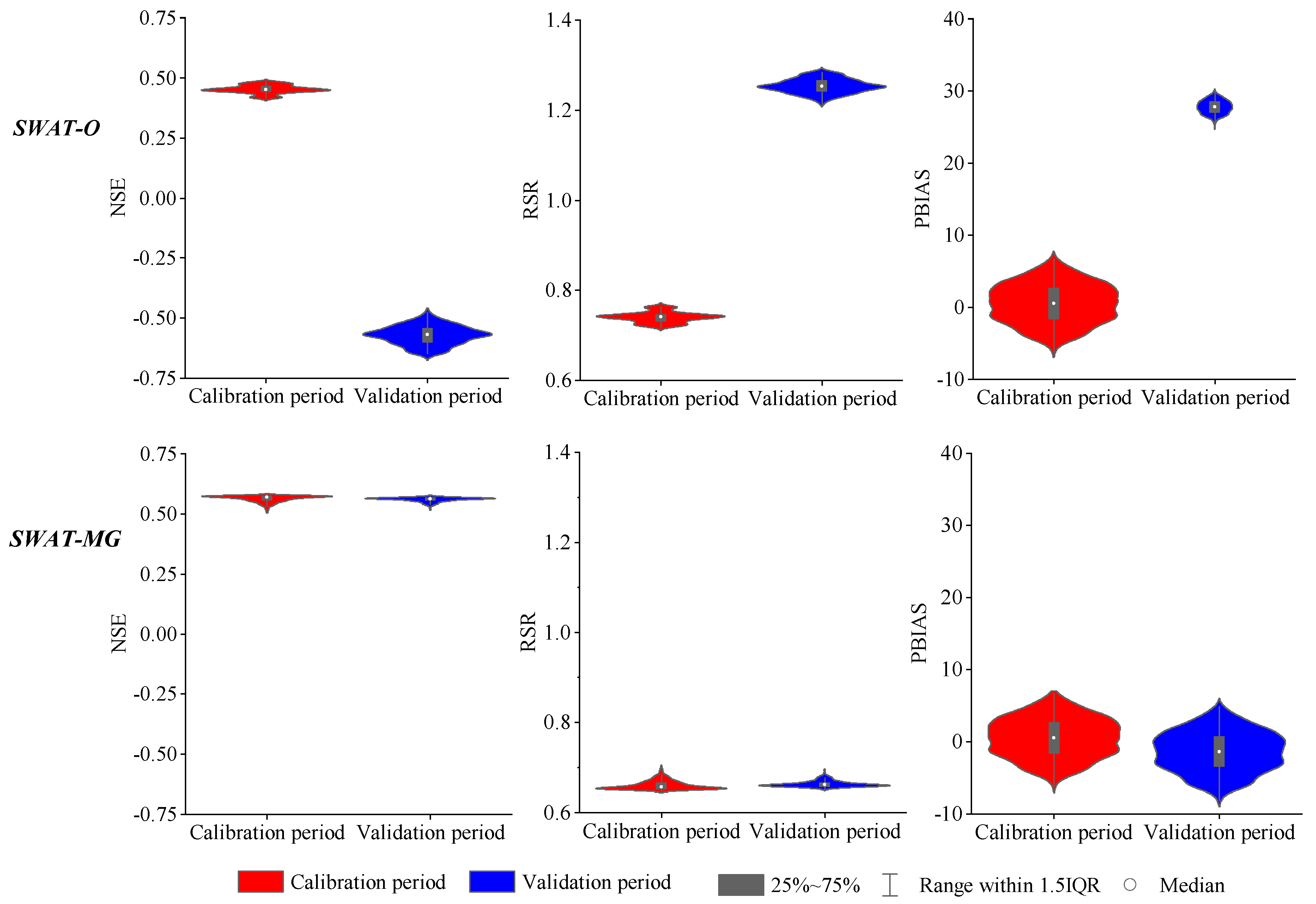
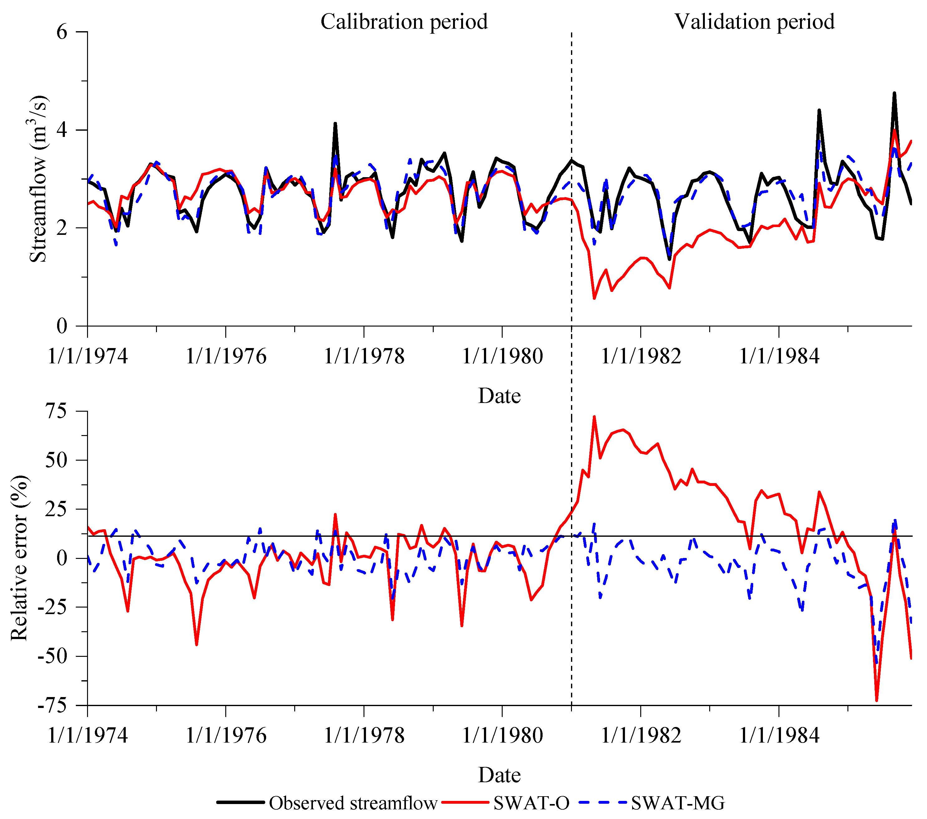
| Criteria | NSE | RSR | PBIAS | ||||
|---|---|---|---|---|---|---|---|
| SWAT Version | |||||||
| Daily | Monthly | Daily | Monthly | Daily | Monthly | ||
| Calibration period | |||||||
| SWAT-O | 0.47 | 0.60 | 0.73 | 0.64 | 0.67 | 0.67 | |
| SWAT-MG | 0.58 | 0.81 | 0.65 | 0.43 | 1.21 | 1.21 | |
| Validation period | |||||||
| SWAT-O | -0.52 | -1.88 | 1.23 | 1.69 | 26.6 | 26.6 | |
| SWAT-MG | 0.57 | 0.71 | 0.65 | 0.53 | -0.93 | -0.93 | |
| Year | Streamflow | Base Flow | SURFACE FLOW | Base Flow /Streamflow (%) | ||
|---|---|---|---|---|---|---|
| Deep Flow | Lower Flow | Upper Flow | ||||
| 1974 | 2.57 | 0.13 | 2.33 | 0.04 | 0.07 | 97.38 |
| 1975 | 2.74 | 0.17 | 2.45 | 0.04 | 0.08 | 97.12 |
| 1976 | 2.68 | 0.18 | 2.36 | 0.04 | 0.08 | 96.9 |
| 1977 | 2.75 | 0.19 | 2.39 | 0.07 | 0.11 | 96.13 |
| 1978 | 2.93 | 0.19 | 2.53 | 0.08 | 0.13 | 95.72 |
| 1979 | 2.82 | 0.2 | 2.51 | 0.04 | 0.07 | 97.34 |
| 1980 | 2.58 | 0.19 | 2.32 | 0.02 | 0.05 | 98.17 |
| 1981 | 2.61 | 0.19 | 2.27 | 0.07 | 0.08 | 96.92 |
| 1982 | 2.63 | 0.19 | 2.28 | 0.08 | 0.08 | 96.87 |
| 1983 | 2.61 | 0.19 | 2.33 | 0.02 | 0.06 | 97.72 |
| 1984 | 2.8 | 0.2 | 2.36 | 0.1 | 0.13 | 95.18 |
| 1985 | 2.99 | 0.21 | 2.62 | 0.05 | 0.11 | 96.18 |
| Average | 2.72 | 0.19 | 2.4 | 0.05 | 0.09 | 96.78 |
© 2019 by the authors. Licensee MDPI, Basel, Switzerland. This article is an open access article distributed under the terms and conditions of the Creative Commons Attribution (CC BY) license (http://creativecommons.org/licenses/by/4.0/).
Share and Cite
Shao, G.; Zhang, D.; Guan, Y.; Xie, Y.; Huang, F. Application of SWAT Model with a Modified Groundwater Module to the Semi-Arid Hailiutu River Catchment, Northwest China. Sustainability 2019, 11, 2031. https://0-doi-org.brum.beds.ac.uk/10.3390/su11072031
Shao G, Zhang D, Guan Y, Xie Y, Huang F. Application of SWAT Model with a Modified Groundwater Module to the Semi-Arid Hailiutu River Catchment, Northwest China. Sustainability. 2019; 11(7):2031. https://0-doi-org.brum.beds.ac.uk/10.3390/su11072031
Chicago/Turabian StyleShao, Guangwen, Danrong Zhang, Yiqing Guan, Yuebo Xie, and Feng Huang. 2019. "Application of SWAT Model with a Modified Groundwater Module to the Semi-Arid Hailiutu River Catchment, Northwest China" Sustainability 11, no. 7: 2031. https://0-doi-org.brum.beds.ac.uk/10.3390/su11072031