Spatial Pattern of the Unidirectional Trends in Thermal Bioclimatic Indicators in Iran


1
School of Civil Engineering, Faculty of Engineering, Universiti Teknologi Malaysia (UTM), Johor Bahru 81310, Malaysia
2
Centre for Coastal and Ocean Engineering (COEI), Universiti Teknologi Malaysia (UTM), Kuala Lumpur 54100, Malaysia
3
State Key Laboratory of Hydrology-Water Resources and Hydraulic Engineering, Nanjing Hydraulic Research Institute, Nanjing 210029, China
4
Research Center for Climate Change, Ministry of Water Resources, Nanjing 210029, China
*
Authors to whom correspondence should be addressed.
Sustainability 2019, 11(8), 2287; https://0-doi-org.brum.beds.ac.uk/10.3390/su11082287
Submission received: 5 March 2019
/
Revised: 25 March 2019
/
Accepted: 26 March 2019
/
Published: 16 April 2019
(This article belongs to the Special Issue Uncertainty of Climate Change Impacts on Hydrology, Water Quality and Ecology)
Abstract
:Changes in bioclimatic indicators can provide valuable information on how global warming induced climate change can affect humans, ecology and the environment. Trends in thermal bioclimatic indicators over the diverse climate of Iran were assessed in this study to comprehend their spatio-temporal changes in different climates. The gridded temperature data of Princeton Global Meteorological Forcing with a spatial resolution of 0.25° and temporal extent of 1948–2010 was used for this purpose. Autocorrelation and wavelets analyses were conducted to assess the presence of self-similarity and cycles in the data series. The modified version of the Mann–Kendall (MMK) test was employed to estimate unidirectional trends in 11 thermal bioclimatic indicators through removing the influence of natural cycles on trend significance. A large decrease in the number of grid points showing significant trends was noticed for the MMK in respect to the classical Mann–Kendall (MK) test which indicates that the natural variability of the climate should be taken into consideration in bioclimatic trend analyses in Iran. The unidirectional trends obtained using the MMK test revealed changes in almost all of the bioclimatic indicators in different parts of Iran, which indicates rising temperature have significantly affected the bioclimate of the country. The semi-dry region along the Persian Gulf in the south and mountainous region in the northeast were found to be more affected in terms of the changes in a number of bioclimatic indicators.
1. Introduction
The bioclimate provides information about annual and seasonal climatic conditions including mean, range, inter- and intra-annual variability and seasonality, and thus is useful for understanding the relationship between climate and living organisms [1]. It can be used to define human comfort [2], agricultural potential [3], species distribution [4], public heat risk [5], pollution susceptibility [6], climate change vulnerability and adaptation needs [7], and therefore, considered important for sustainability. A number of climate factors including temperature, humidity and wind and their variations affect the energy balance of the human body and comfort levels [2]. Therefore, bioclimatic indices are widely used to map the geographical distribution of human comfort zones [8,9]. It has also been used to define the potential of an area for the growing of a particular variety of crop [3]. Villordon et al. [10] used a bioclimate concept to map the potential zones for growing sweet potato in sub-Saharan Africa. Nabout et al. [11] identified suitable maize cultivation lands using bioclimatic factors. Most of the species can sustain in a bioclimatic niche, and thus, a small shift in the bioclimate may significantly change the distribution of species and ecology of a region [4,12]. The relationships of bioclimate with public health are also well-established through a number of studies [5,13,14]. It has been found that the outbreak of a number of diseases and mortality are significantly correlated to different bioclimatic factors. Certain bioclimatic conditions are found to be favourable for stagnant pollution and degradation of environmental quality [6]. The bioclimate of a region can also tell the vulnerability of the region to climatic hazards [7]. In addition, it has been used for architectural design of buildings [15], urban planning [16] and climate change adaptation strategizing [17,18]. A wide range of applicability and effectiveness have made it an attractive tool for the evaluation of the relationship of climate with humans, the environment and ecology.
Climate change has altered not only the mean temperature and rainfall but the seasonality, intra-annul variability and other properties of climate. These have also changed the favourable bioclimate for human health and ecological niche of a region. The use of bioclimatic indicators to assess the ecological responses to climate change and its impacts on bio-environments have grown rapidly in recent years [18,19,20,21]. Understanding the ongoing changes in the bioclimate can help in adaptation planning to mitigate the impacts of changes in climate and sustainable management of bio-environment [22,23].
Climatic trends are usually assessed to quantify the changes in climate. The Mann–Kendall (MK) trend test is generally used for this purpose. Though this non-parametric method has a number of advantages over other methods, the major drawback of the method is the influence of autocorrelation in data on its test significance. A number of modifications in the MK test has been proposed to remove the influence of autocorrelation through pre-whitening of data. However, recent studies have suggested that those are not sufficient enough to exclude the effect of long-term dependency on the data series on MK trend significance [24,25]. The long-term autocorrelation which may appear in the time-series due to multi-decadal climate variability can also overestimate the MK trend significance [26,27]. Therefore, the trends estimated by the MK test may not always be the unidirectional trend [28,29]. This fact has been established in recent studies through the analysis of hydro-climatic trends in different regions [28,30,31,32]. The Intergovernmental Panel for Climate Change (IPCC) [33] also indicated that some climatic trends reported in different parts of the globe may not be valid, due to the long-term self-similarity in the data. Hamed [26,34] modified the MK (MMK) test to improve its ability in trend analysis through consideration of long-term dependency in data, and thus, its capacity to distinguish the natural climate variability from monotonic trends. The MMK test has been used in recent years to assess unidirectional trends due to the presence of global warming [7,28,35,36,37,38].
A large number of bioclimatic indicators have been developed to relate climate with the biosphere [39]. The thermal bioclimatic indicators are supposed to be affected more by global warming due to sharp increases in global temperature. Therefore, the assessment of the changes in thermal indicators is very urgent. The changes in climate, and thus, bioclimate widely vary for different climatic regions. The evaluation of trends in thermal bioclimatic indicators over a diverse climate can provide important information related to global warming induced climate change impacts on bioclimates in different climatic regions.
Trends in thermal bioclimatic indicators over the diverse climate of Iran are assessed in this study with an intention to comprehend the impacts of climate change on thermal bioclimate in different climatic zones. Though numerous studies have assessed trends in different climatic variables of Iran, the assessment of the trends in bioclimatic indicators is still limited [6,40,41]. In recent years, a number of studies have been conducted to assess of geographical distribution of bioclimatic conditions [42,43,44,45,46]. Trends in few of the thermal bioclimatic indicators such as annual average temperature and diurnal temperature range (DTR) have been well analysed in those studies. But all those studies used the MK test or the modified version of the MK test that consider only short-term autocorrelation in data. The MMK test was used in this study to assess the unidirectional trends in 11 thermal bioclimatic indicators due to the presence of global warming. Trends in some of the indicators were assessed for the first time. The obtained results were compared with those estimated using the MK test. Gridded monthly temperature data of the Princeton Global Meteorological Forcing (PGF) with a spatial resolution of 0.25° was used for the mapping of the spatial pattern in the trends for the period 1948–2010. It can be expected that the application of the MMK test using long-term high-resolution climate data over a diverse climate will provide valuable information on anthropogenic climate change impacts on thermal bioclimates.
2. Description of the Study Area and Data Sources
2.1. Topography and Climate of Iran
Iran, located in Southwest Asia (Lat: 25°–40° N; Lon: 44°–61° E), covers an area of 1.648 million km2. The topography of the country varies widely from −24 m in the northern coastal region along the Caspian Sea to 5500 m in the central and northern mountainous regions (Figure 1). Highlands and mountain ranges dominate most parts of the country. The major topographical features of the country include two major mountain ranges, one in the north (The Alborz) and the other extending from the northwest to the southwest (The Zagros); two long coastlines in the north and south; and two vast deserts, Kavir and Lut, in the central east and central north of the country. The large variations in topography have made the climate of the country highly diverse. Figure 2 shows the climate zones of Iran. Alizadeh-Choobari and Najafi [47] classified the climate of Iran into six zones based on rainfall, namely, extremely dry in the central, eastern and south-east regions; dry in an extended region from the centre to the east; semi-dry in the northwest, northeast, southwest and west; semi-wet in the west and north; and wet and extremely wet in the northern coastal region. Overall, the semi-dry or dry climate dominates the most parts of Iran.
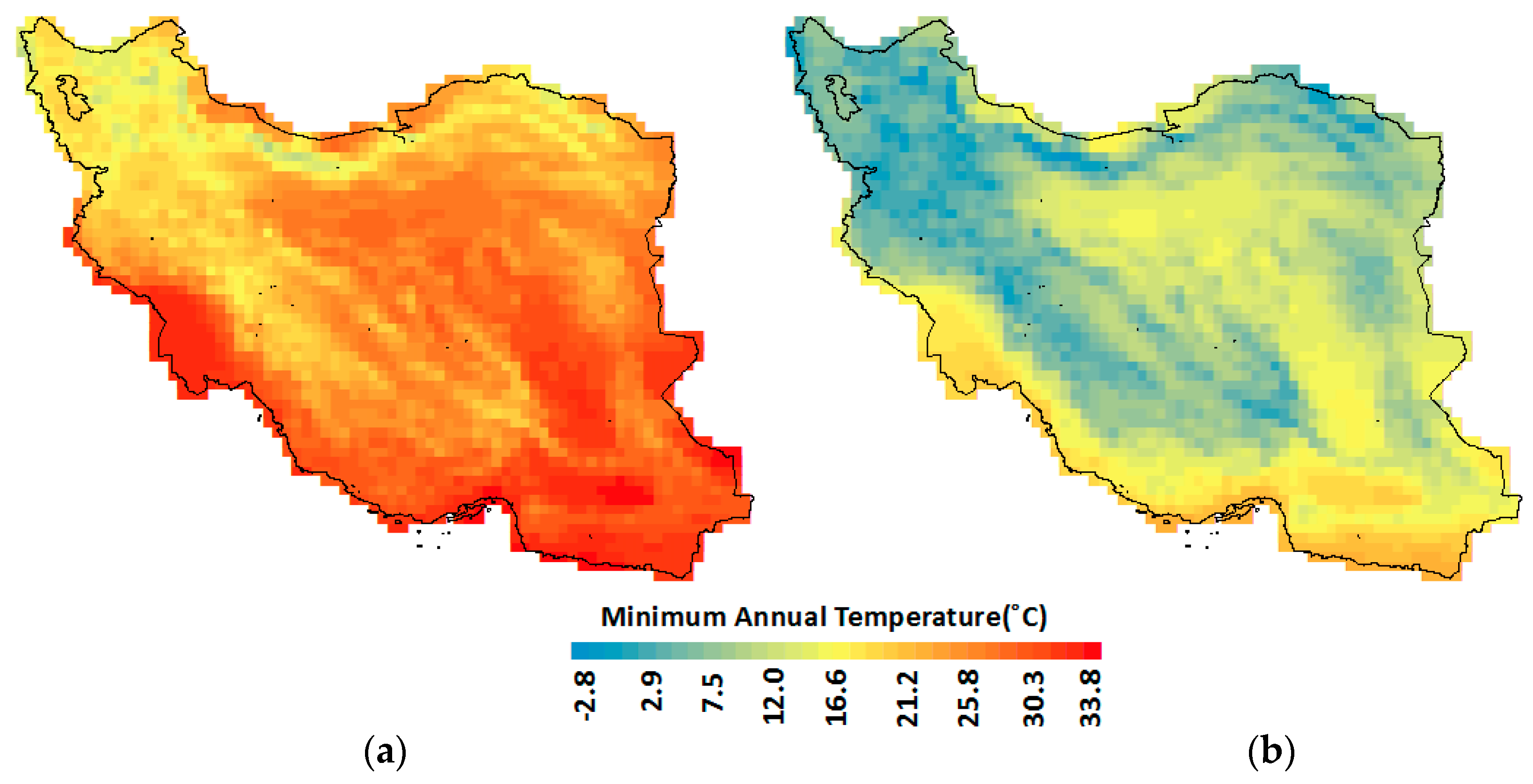
The annual average daily maximum temperature of Iran varies from 1.4 °C in the northwest mountainous region to 33.8 °C along the Persian Gulf coastal region in the south. However, annual maximum temperature in most parts of the country except the deserts and coastal region does not go beyond 25 °C. The annual average of daily minimum temperature ranges from sub-zero (−2.8 °C) in northwest mountainous region to 21.9 °C in the southern coastal region.
2.2. Princeton Global Meteorological Forcing Data
The monthly average of daily mean, maximum and minimum temperature data of PGF were used in this study for the estimation of thermal bioclimatic indicators. Besides, PGF temperature data, rainfall data having the same resolution was used in this study for the identification of wet and dry periods for the estimation of two bioclimatic indicators. The PGF temperature dataset [48] was developed using NCEP (National Centres for Environmental Prediction) reanalysis temperature data and global observed temperature. It provides global coverage of monthly and daily temperatures for the period 1948–2010 with a spatial resolution of 0.25°. Details of the development and properties of PGF are given in Sheffield et al. [48].
The monthly data of PGF were extracted from 2484 grid points for the period 1948–2010 to cover the entirety Iran. The quality of the extracted PGF data was assessed using available observed data. For this purpose, the long-term temperature records (1951–2010) available at different locations of Iran was compared with PGF temperature data of the nearest grid point. High correlation between the observed and the PGF temperature was found at all the locations. In addition, visual inspection through scatter plots revealed good agreement between the observed and the PGF temperature, and thus, the suitability of the PGF temperature data for the analysis of thermal bioclimatic trends in Iran. The PGF data has also been found suitable for trend analysis in a number of studies at global [49,50] and regional [7,32,51,52] scales, including in Asia [7,37,53,54,55].
The spatial distribution of annual average daily maximum and minimum temperatures in Iran prepared using PGF monthly temperature for the period 1948–2010 is shown in Figure 3a,b, respectively.
3. Methodology
3.1. Thermal Bioclimatic Indicators
Trends in 11 thermal bioclimatic indicators were assessed in the present study. The descriptions of the indicators are given in Table 1. The units of all the indicators are in °C except Bio3, which is in percentage. Therefore, the changes in the indicators are presented in this paper using absolute values (°C/decade) instead of percentage of change, which is often used to present the changes in rainfall [56,57]. The monthly average of daily maximum and minimum PGF temperature data for the period 1948–2010 were used in the present study for the estimation of annual time-series of each of the thermal bioclimatic indicator at each grid point.
3.2. Autocorrelation and Natural Variability in Climate
The characteristics of temperature data were analysed to see the presence of autocorrelations and multi-decadal variability in data. The analyses were done to justify the use of the MMK test. The autocorrelation function (AFC) was used in this study to find the significant correlation for various time lags. For temperature data, Y1, Y2, …, YN measured at an equal time interval, the autocorrelation function for lag, k can be estimated as [58],
The presence of decadal and multi-decadal variability in temperature time-series was evaluated through wavelet decomposition of time-series data [59,60]. The wavelet function (ψ) of non-dimensional time parameter (η) of a temperature time-series Y(t) with time, t ranging between −∝ and +∝, can be expressed as [61],
where τ is the time step on which the wavelet is repeated over Y(t) and s is a measure varying between 0 and ∝. The ψ(η) is localized in time–frequency space with a mean of zero [62]. In this study, ψ(η) was estimated for a different value of τ to decipher the occurrence of different cycles in the time-series.
3.3. Estimation of the Changes and Significance
The changes in bioclimatic indicators were estimated using Sen’s slope method. The significance of the changes for a particular confidence level was estimated using the MK and MMK tests. The methods are described below.
3.3.1. Sen’s Slope for Estimation of the Changes
The Sen’s slope [63] is a non-parametric robust estimator of change [56,64]. It first estimates the changes (s) between all consecutive data points of a time-series,
where ΔY is the difference in two data measures at an interval of Δt. The Sen’s slope is computed as the median of all the changes (s) to describe the change per unit time over the whole period.
3.3.2. MK Trend Tests
The Mann–Kendall test [65,66] is a robust trend test endorsed by the World Meteorological Organisation (WMO) for hydro-climatic trend analysis [67]. If Y(t) is a temperature series with N measurements, Y1, Y2, Y3, … and YN, the MK statistic (S) for the series is,
The trend significance is computed using normalised test statistic (Z) from S and its variance Var(S),
The sign of Z indicates the direction of trend and the absolute magnitude to Z is used to estimate the confidence interval of trend (|Z| > 2.58 and 1.96 represent 99% and 95% confidence interval, respectively).
3.3.3. MMK Trend Tests
The MMK test first assesses the trend using the MK test. If the MK test finds a significant trend in the time-series, the MMK test de-trends the series and ranks the data (Ri) to estimate its equivalent normal variants () using the inverse standard normal distribution function (),
The Z is then used to compute the Hurst coefficient (H) using the maximum log likelihood function [68],
where is the determinant of the correlation matrix of lag for a given H; and represent the transpose and variance of Z. The H that yields maximum value of in Equation (8) is calculated to determine the present of long-term dependency in the time-series. The significance of H is computed using the mean and standard deviation for H = 0.5. The biased estimate of Var(S) ( is computed when H is found significant,
where is the auto-correlation function for a given H. The unbiased estimate, is calculated from a biased estimate by multiplying with B, which is a function of H,
The procedure used for the estimation of B is given by Hamed [26]. For the estimation of the significance of the MMK test, the is replaced with in Equation (6).
3.4. Mapping the Geographical Distribution of Trends
The Sen’s slope and the trend test statistics in different PGF grid points were used for the mapping of the spatial pattern in the trends of thermal bioclimatic indicators using ArcGIS10.3. In the present study, points and areas filled with colour were used to represent the significance and magnitude of trend at each PGF grid point. Different colours were used to show the rate of change in °C/decade, while the dots were used to show the significance of trend. The black and white dots were used to show trends at the 95% confidence level using the MK and MMK, test respectively.
4. Results
4.1. Autocorrelation and Natural Variability in Climate
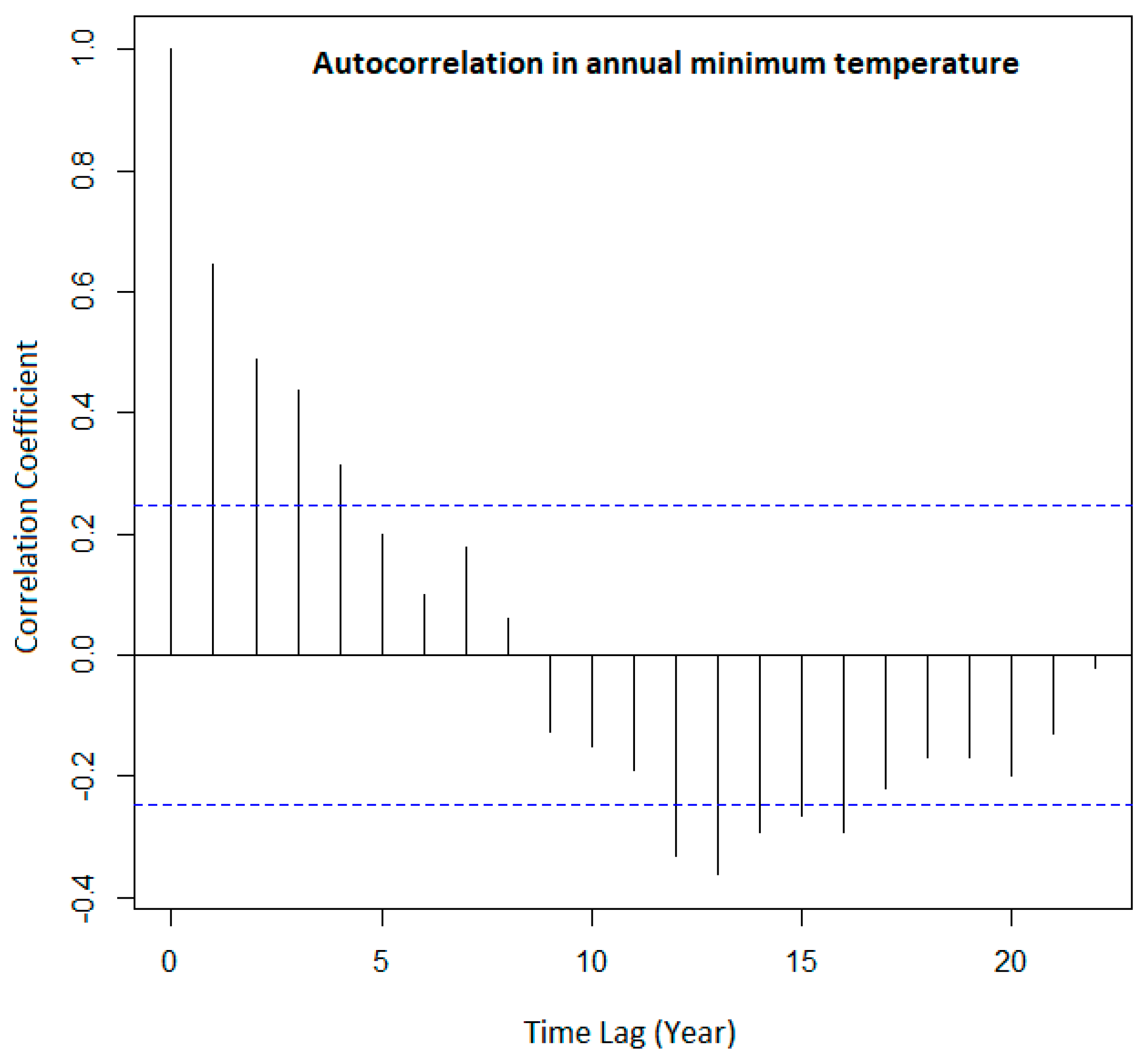
The autocorrelation function (ACF) plot of annual average daily minimum temperature at a grid point (55.25° E; 33.5° N) is shown in Figure 4. The vertical lines in the plot that exceed the blue confidence band indicate significant correlation. The figure clearly shows positive autocorrelation up to 16-lag years in the time-series. Similar results were obtained at many other grid points for both maximum and minimum temperature time-series. The results indicate the presence of short- and long-term autocorrelations in the temperature time-series of Iran.
The annual temperature time-series was decomposed to different levels using a wavelet decomposition technique to show the presence of different cycles in the time-series. Different levels of decompositions revealed different cycles. The fourth-level decomposition of temperature data revealed the presence of a long-term cycle, as shown in Figure 5. The figure shows a multi-decadal cycle with varying length. The figure clearly shows the presence of long-term variability in the temperature data series. Similar long-term variability was noticed in temperature time-series at many other grid points. Such long-term variations in annual temperature time-series can significantly affect the trend in bioclimatic indicators if it is not taken into consideration during trend analysis.
4.2. Areal Coverage of Trends in Thermal Bioclimatic Indicators
The trends in bioclimatic indicators were estimated using the MK and MMK tests for the 95% and 99% levels of confidence at each grid point. Obtained results at different grid points were used to estimate the percentage of total grid points over Iran for which different indicators were changing significantly. The percentage of grid points at which different thermal bioclimatic variables showed increasing or decreasing trends at 95% and 99% confidence intervals are given in Table 2. The table shows a large difference between the results obtained using the MK and MMK test. The number of grid points showing significant change was found to be reduced considerably for the MMK test. The results clearly prove that many of the trends were due to the presence of different forms of autocorrelations in temperature time-series.
Table 2 shows an increase in annual mean temperature (Bio1) over a large part of Iran, 96.3% and 38.0% area by the MK and MMK tests, respectively, at the 95% level of confidence. The increases were also found significant at the 99% level of confidence at 92.6% and 20.3% of the grid points. The Bio2 was found to decrease at 40% and 3.3% grid points by the MK and MMK tests at the 95% level of confidence. Increase in Bio2 was also observed but at fewer number of grid points. This indicates that minimum temperature increased more compared to maximum temperature at many grid points. The increase in Bio1 over a large area and decrease in Bio2 in a significant number of grid points by MMK indicate the evidence of global warming in Iran. The increase in temperature caused a change in different thermal bioclimatic indicators in Iran. The Bio3 was found to decrease, while all others (Bio4 to Bio11) were found to increase at a number of grid points by both the MK and MMK tests, except Bio6 which was not detected to change at any grid point by MMK. The Bio10 was found to increase at the highest number of grid points (45.5% by MMK test), while Bio3 was found to decrease at the highest number of grid points (6.5%).
4.3. Spatial Distribution of the Trends in Thermal Bioclimate Indicators
The trends obtained in thermal bioclimatic indicators at different PGF grid points were used to generate the maps in order to present the spatial distribution of the trends in thermal bioclimatic indicators over Iran. A common legend was used to show the changes in all bioclimatic indicators except Bio3 (due to different unit) in order to facilitate an easy comparison of the changes in different indicators. A colour ramp (green to yellow to red) was used to show the amount of change in indicators in each grid box estimated using Sen’s Slope method, where yellow to red colour was used to show the positive trend and yellow to green was used to present the negative trend. A dot in the centre of grid box was used to represent the significance of trends. A black dot was used to show the significant trend obtained using the MK test, while a white dot was used to show the location where the MMK test estimated a significant trend. Trends were evaluated in this study for both the 95% and 99% level of confidence. However, only the trends obtained at a 95% confidence level are presented and discussed in the following sections. The map showing the spatial distribution of the indicators were also prepared along the map of their trends for better description of the changes. A yellow-to-dark-brown colour ramp was used to show the spatial distribution of the indicators.
4.3.1. Annual Mean Temperature (Bio1)
The spatial distribution of Bio1 and its trends estimated at different grid points over Iran are shown in Figure 6a,b, respectively. The Bio1 in Iran varies from 6.7 °C in the far north to 27.4 °C in the southern coastal region. The spatial distribution of Bio1 is heavily influenced by topography. It was found less in the mountainous regions and higher in the plain desert and coastal regions. A significant increase in Bio1 in the range of 0.3 to 0.45 °C/decade was observed in Iran. The increase was found much higher in the desert in the east and southwest coastal region. Overall, the temperature rise in Iran was found much higher than the global average of 0.15 °C/decade after 1970. This indicates that temperature in some parts of Iran, particularly those are located in the dry and semi-dry regions, are increasing very fast. The MK test revealed the increases were significant in most parts of the country at the 95% level of confidence, except the wet regions in the north and in a strip in the semi-dry southern coast. The MMK test showed a large decrease in the number of grid points showing significant changes. It showed an increase in Bio1 in about 38% of the grid points over the country, mostly concentrated in semi-dry and wet regions in the north and the central parts of the country. Besides, an increase in Bio1 was found in the eastern region having an extremely dry climate. Overall, the MMK test revealed that global warming induced temperature rises are already visible in the semi-dry and wet regions of the country.
4.3.2. Diurnal Temperature Range (Bio2)
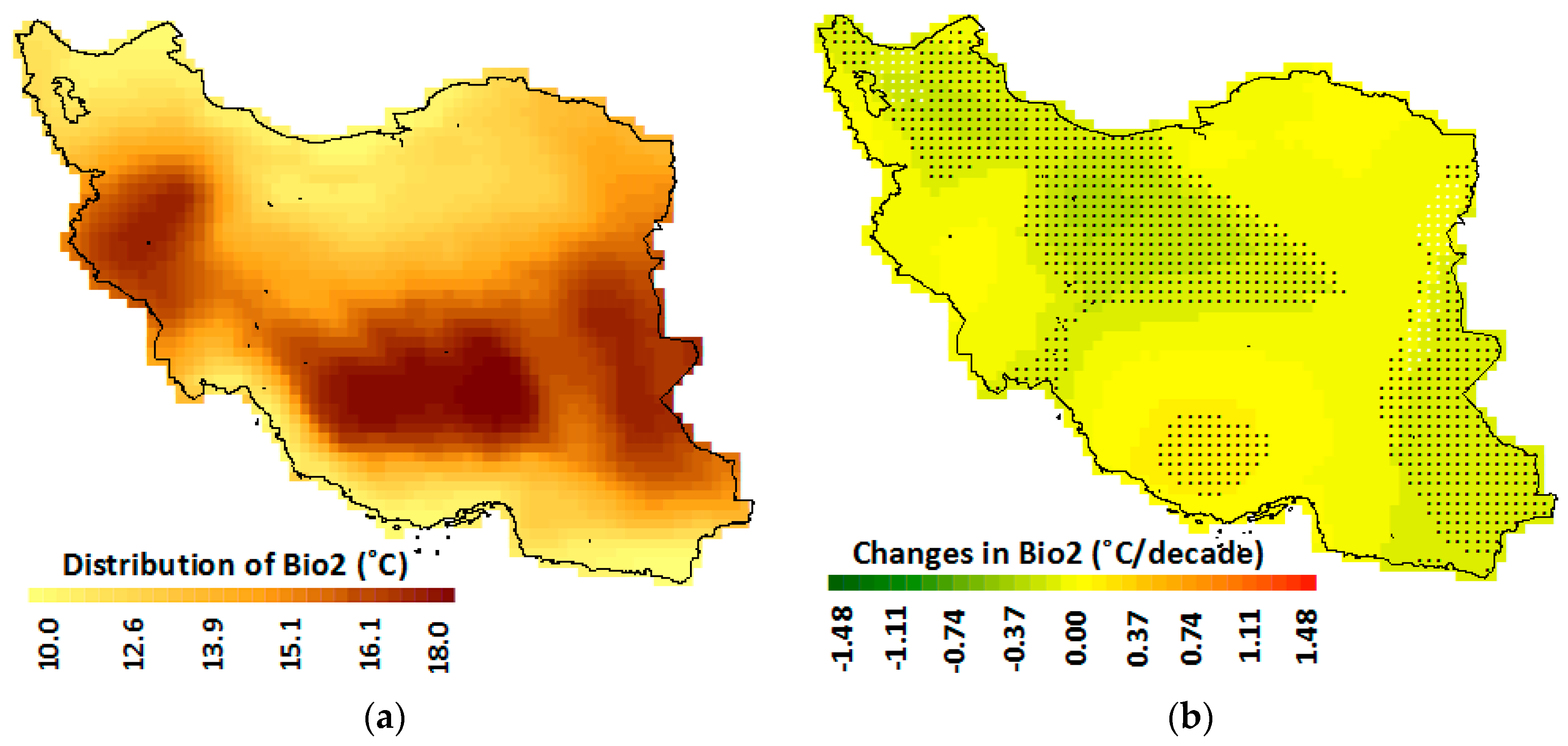
The Bio2 is often considered as an indicator of the climate change footprint of an area, as it does not depend on internal variability of climate [69,70,71]. Increase in minimum temperature has been found more compared to maximum temperature, and thus, a decrease in Bio2 has been found in many regions of the world, which has been linked to global climate change in a number of studies [70,71]. The present study also revealed a decrease in Bio2 in Iran (Figure 7). The MK test showed a decrease in Bio2 in the semi-dry and wet regions in the north and south, and the extremely dry region in the east, while the MMK test showed a decrease in Bio2 only in 3% of the grid points located in the semi-dry region in the far north and in the dry and extremely dry climatic zones in the east bordering Pakistan. The results revealed the impacts of climate change driven by global warming are already evident in Iran.
4.3.3. Isothermally (Bio3)
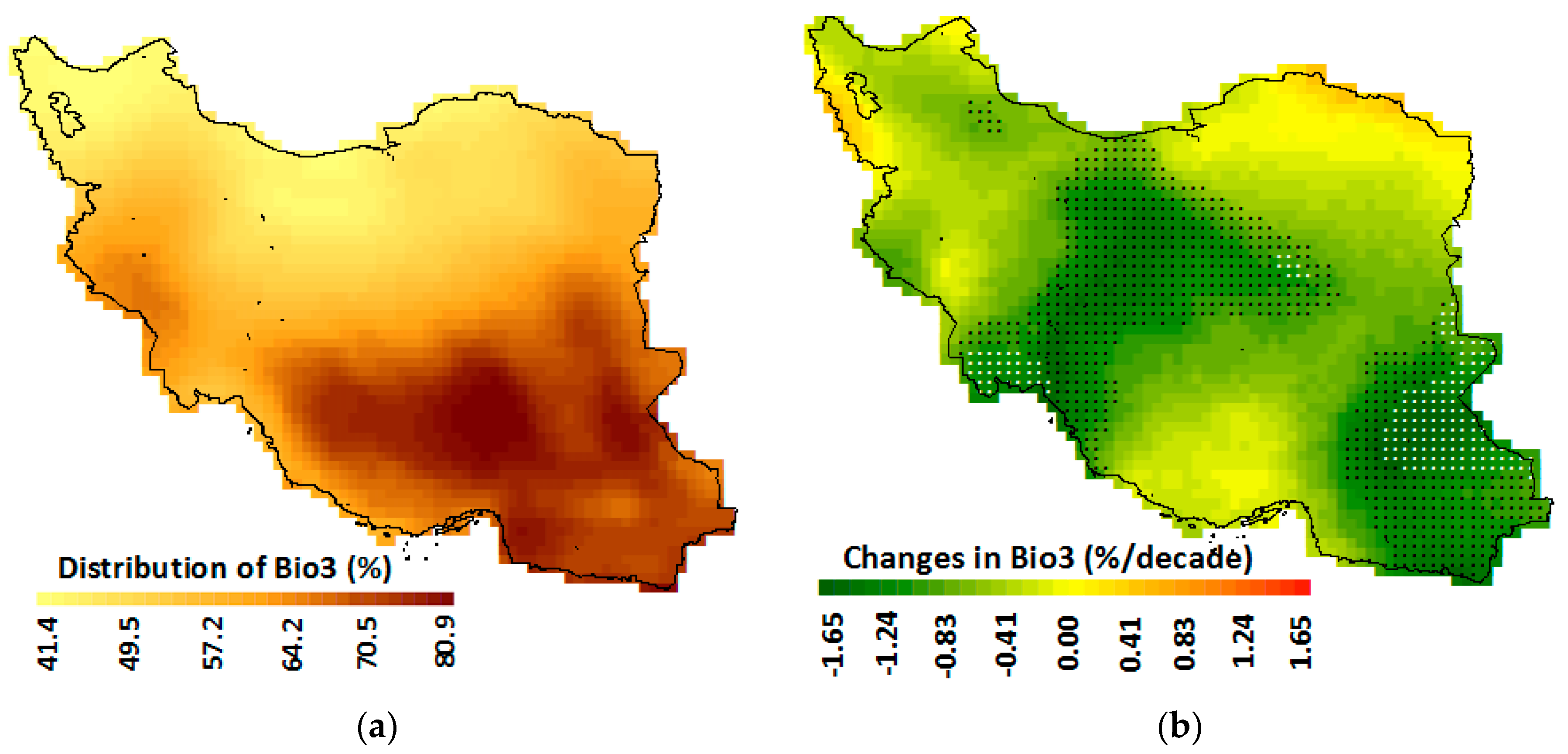
Figure 8a,b shows the spatial distribution of Bio3 and its trends over Iran, respectively. Isothermality is an important bioclimatic indicator for tropical and maritime regions [72]. It is estimated as the ratio of the DTR to annual temperature range (ATR) and expressed in percentage. A Bio3 of 100 means the DTR is equal to the ATR. Therefore, a Bio3 less than 100 means lower variability of diurnal temperature compared to annual variability of temperature. The Bio3 in Iran varies from 41.4 to 80.9% (Figure 8a). It is less than 50% in most parts of the country, particularly in the north half, while it varies between 65 to 80% in the south. The trends in Bio3 revealed a decrease in some regions of the country. It means a gradual decrease in diurnal temperature variability compared to annual temperature variability in some parts of Iran. This is mainly due to the decrease in DTR. The MK test showed a decrease in Bio3 in a large area in the central and the southeast. The most drastic drop in the number of significant grid points from the MK to MMK tests was observed for Bio3. The MMK test revealed a decrease in Bio3 only in three small patches located in the southeast, central and southwest coastal region at the 95% level of confidence. The results showed that Bio3 was decreasing in the region where it was already less.
4.3.4. Temperature Seasonality (Bio4)
The spatial distribution of Bio4 and its trends in Iran are shown in Figure 9a,b, respectively. The seasonality of temperature is the change of temperature over a year. It captures the dispersion in temperature in relative terms. A larger value of Bio4 indicates more variability of temperature [1]. The Bio4 in Iran varied from 4.6 to 9.5 °C. It was found higher in the north and less in the south, particularly in the southern coastal region where it ranged between 4.6 and 7.2 °C. The MK test revealed an increase in Bio4 mostly in the east, southwest and some parts in central Iran where the climate is dominantly dry and semi-dry. The MMK revealed a significant trend in Bio4 only in the stretch along the Persian Gulf in the southwest and in some small areas in the dry and extremely dry regions in the Kavir dessert. Overall, Bio4 was found to increase in the region where it is less, and thus, indicates more spatial homogeneity in future.
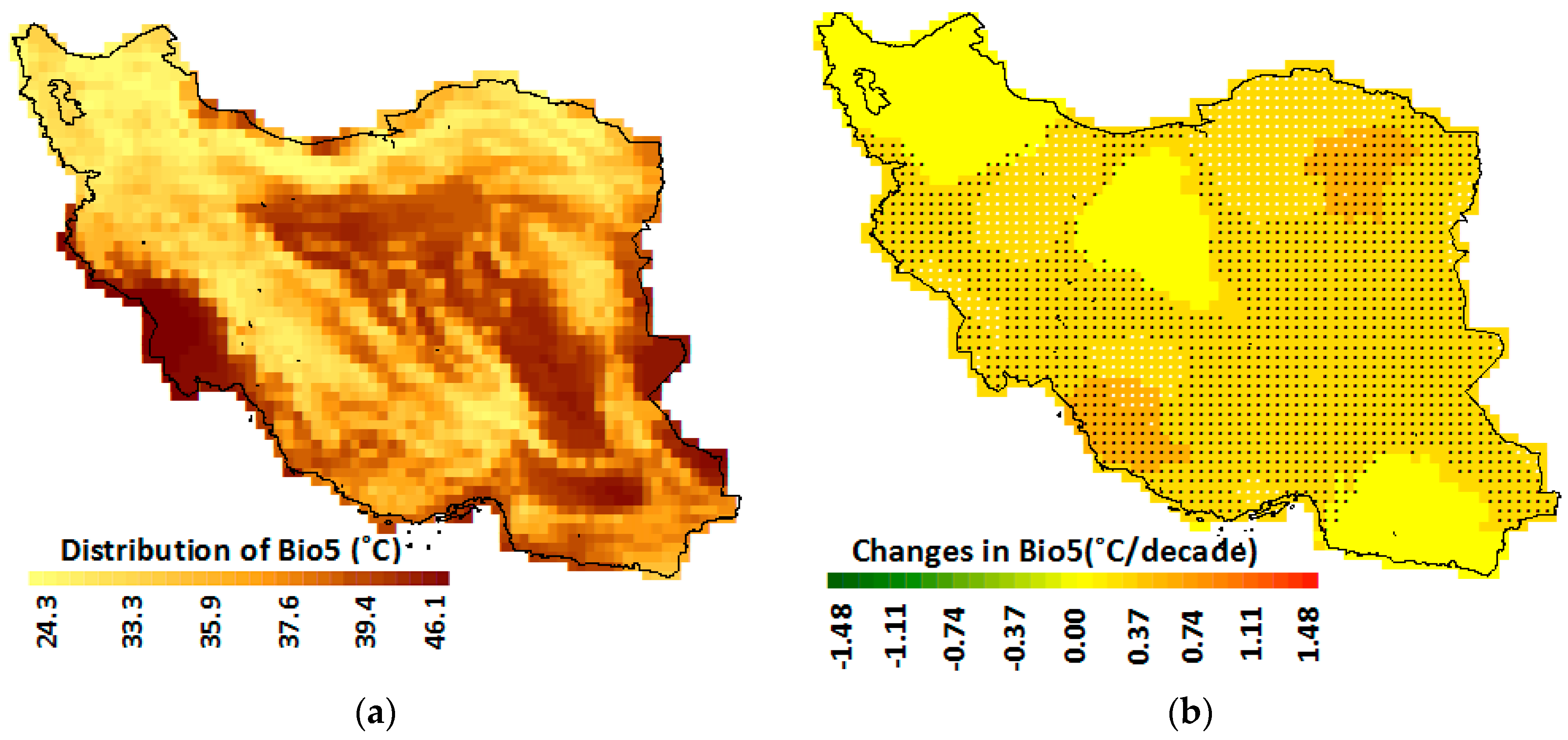
4.3.5. Maximum Temperature in the Warmest Month (Bio5)
The Bio5 varied from 24.3 to 46.1 °C which indicates high temperature in the warmest quarter in Iran (Figure 10a). It was found very high at 39.4 to 46.1 °C in the desert and the southern coastal regions, particularly in the upper part of the Persian Gulf coast. The Bio5 in the far north and the mountainous regions where temperatures are usually less also went above 30 °C. The increase in Bio5 was found by the MK test over the entire country except in the semi-dry climatic region in the northwest and central, and dry climatic region in the southeast (Figure 10b). The MMK test also showed a large increase at a rate of 0.5 °C/decade in the northeast and west of the country. Significant increases were also observed in the northern wet and very wet regions. The results indicated a unidirectional increase in Bio5 in all climatic zones of Iran. Overall, the Bio5 was found to increase in the region where it is usually less, except in the upper part of the Persian Gulf coast where Bio5 is very high. The results indicated more spatial homogeneity in Bio5 in Iran with time.
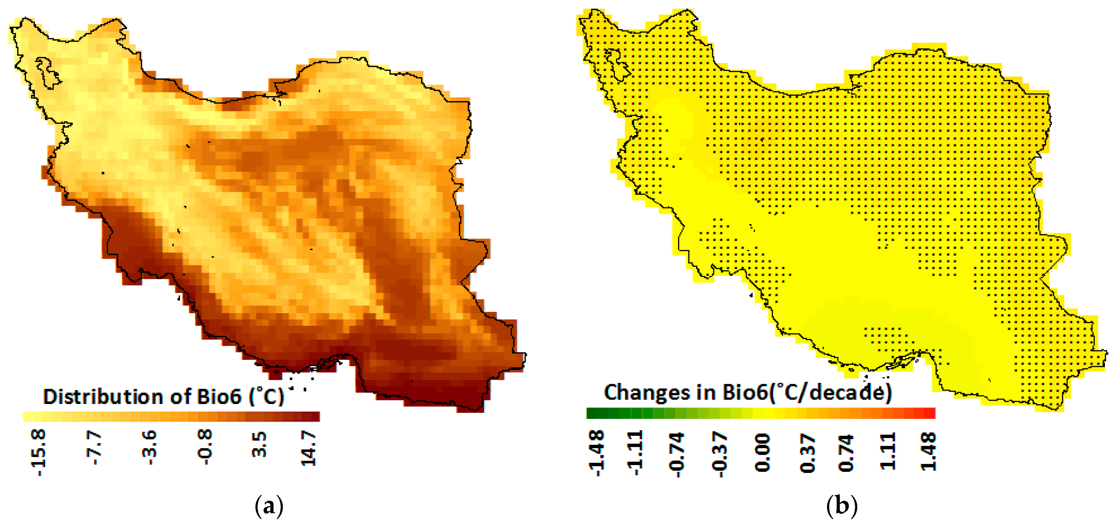
4.3.6. Minimum Temperature in the Coldest Month (Bio6)
The Bio6 had a more or less similar spatial variability as Bio5 (Figure 11a). It varied from −15.8 to 14.7 °C. It was found below zero in most parts of the country except in the desert and the southern coastal regions, with the lowest in the mountainous regions of the far north. The MK test showed an increase in Bio6 in most parts of the country except the semi-dry and dry climate area in the Zagros Mountains extending to the southern coastal region. Compared to the changes in Bio5, the Bio6 was found to increase less in the coldest quarter (Figure 11b). The MK test revealed an increase in Bio6 in the southeast. However, the MMK test revealed that almost none of the trends were significant when natural variability of climate was considered to evaluate the trends. The result of the MMK test indicated minimum temperature in the coldest quarter of Iran was not affected by global warming induced climate change.
4.3.7. Annual Range of Temperature (Bio7)
The Bio7 in Iran ranged from a very high value (>30 °C) in the far north mountainous region to 11.5 °C in the southern coastal region. A large contrast in Bio7 between the north and south can be observed in Iran (Figure 12a). The Bio7 was found to increase in the southeast extremely dry region and in the dry and semi-dry area extended from the Zagros Mountains to southwest coast by 0.42 °C/decade (Figure 12b). The increase above 0.25 °C/decade was detected as significant by the MK test. The MMK test showed that Bio7 was increasing only along the Persian Gulf coast region.
4.3.8. Mean Temperature of the Wettest Quarter (Bio8)
Having a diverse climate, the rainfall distribution in Iran varies widely for different seasons. The wettest quarter in the country, therefore, also varies significantly. In this study, the rainfall for all the consecutive three months at each grid point was estimated to select the wettest quarter at each grid point. The mean temperature during the wettest quarter was estimated to show their spatial distribution (Figure 13a) and trends (Figure 13b).
Heterogeneity was observed in spatial distribution of the trends in Bio8 in Iran. The MK test showed significant trends in Bio8 sporadically distributed over the country. The MMK test showed that Bio8 was increasing significantly only in some areas in the far north, northeast and southeast. The increases were found mostly in the semi-dry and dry regions.
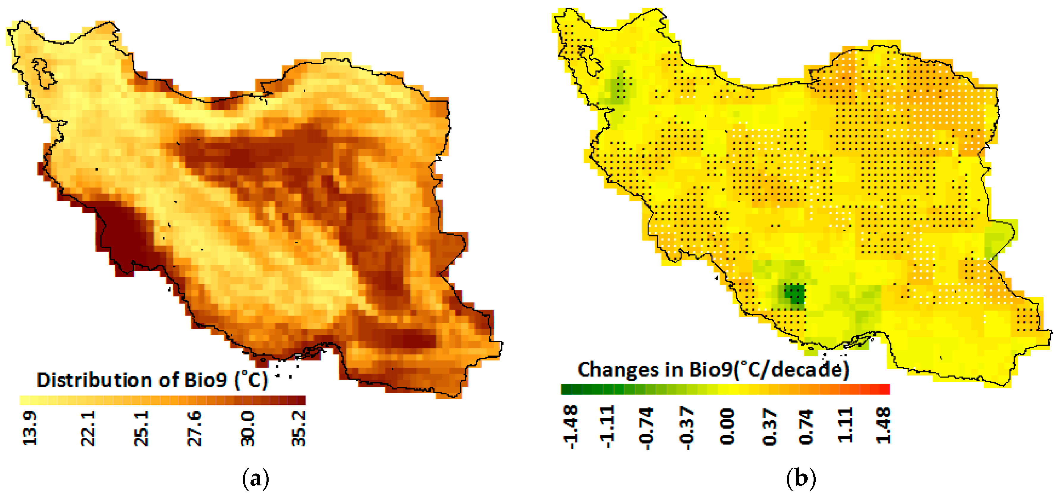
4.3.9. Mean Temperature of the Driest Quarter (Bio9)
The rainfall for all the consecutive three months at each grid point was estimated to select the driest quarter at each grid point. The mean temperature during the driest quarter was used to map their spatial distribution (Figure 14a) and analysis of trends (Figure 14b). The mean temperature during the driest quarter was found to increase over a large area in the east, central and southwest. The MK test showed an increase in Bio9 in 48.1% of the area while the MMK test showed an increase in 14.8% of the area at the 95% confidence interval. The increases were found heterogeneously distributed over the country. Overall, it was found to increase mostly in semi-dry regions in the southwest and northeast.
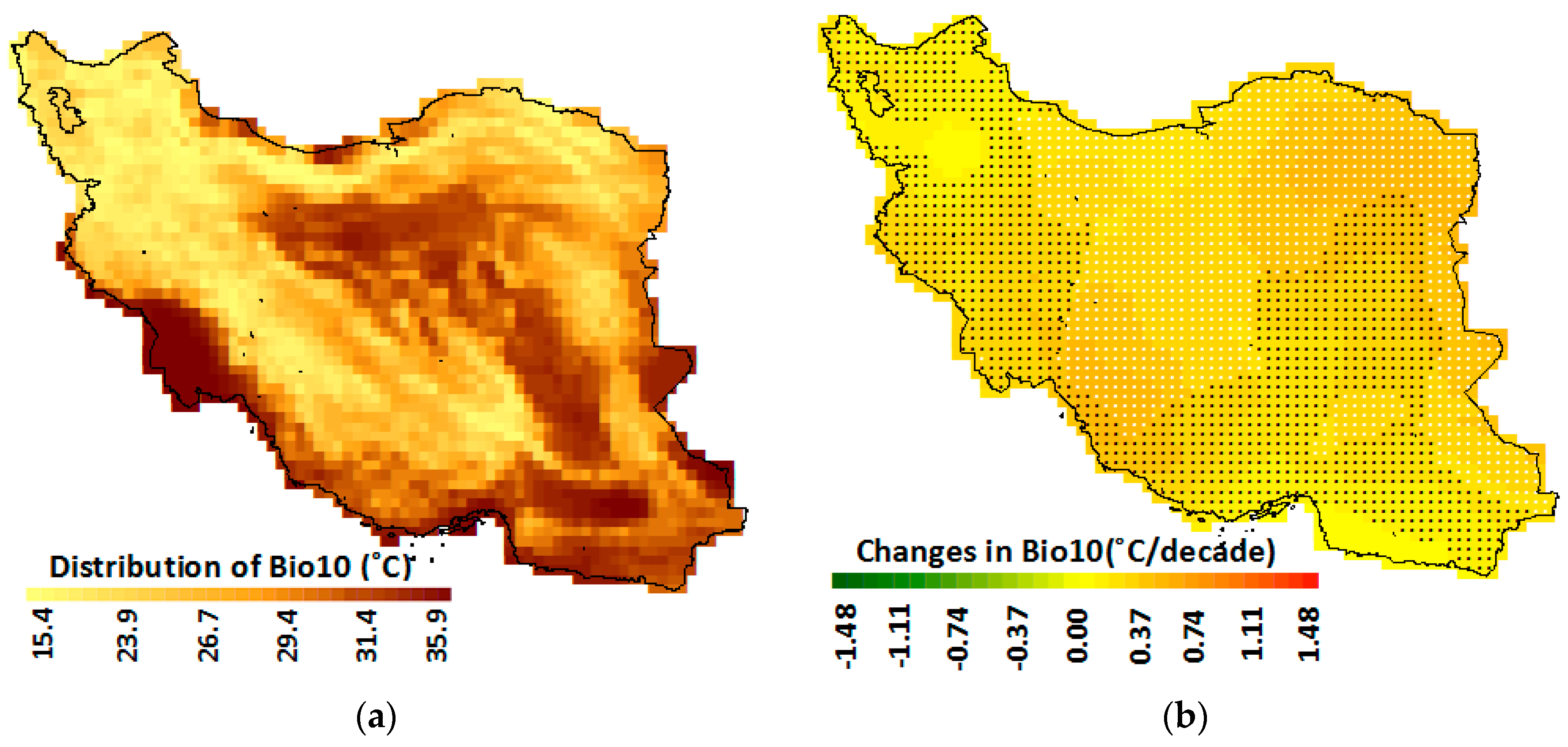
4.3.10. Mean Temperature of the Warmest Quarter (Bio10)
The mean temperature for all the consecutive three months at each grid point was estimated to select the warmest quarter at each grid point. The mean temperature during the warmest quarter for each year was computed to generate the time series of Bio10. The time-series was used to map the spatial distribution of Bio10 and estimate its trend. The spatial distribution and trends in mean temperature during the warmest quarter are shown in Figure 15a,b, respectively.
Bio10 was found to follow the topography of Iran. It was found high in the plain lands and less in mountainous regions. A large increase in Bio10 in the range of 0.2 to 0.6 °C/decade was observed in most parts of Iran. The areal coverage of the increasing trend was 95% for the MK test and 45% for the MMK test at the 95% confidence interval (Table 2). The highest increase was found in the east and the southwest semi-dry and very dry regions. Besides, it was observed to increase significantly by both the MK and MMK tests in the whole north, central and northeast regions. The study clearly indicates a unidirectional increase in mean temperature during the warmest months due to climate change.
4.3.11. Mean Temperature of the Coldest Quarter (Bio11)
The spatial distribution and trends in Bio11 are shown in Figure 16a,b, respectively. It was found to follow a similar pattern of Bio10, high in the plain lands and low in mountainous regions. However, compared to mean temperature in the warmest quarter, it was found to increase less. The MMK test revealed that it was increasing only at a few grids in the northeast semi-dry region and at three grids in the southeast desert. Significant increase in Bio11 was noticed in the range of 0.20 to 0.56 °C/decade. The increases were found in the same regions were Bio10 was increasing but at a smaller areal extent.
5. Discussion
The climate and biological systems are closely interlinked, and thus, the assessment of the changes in bioclimate is vital for the anticipation of the possible changes in interactions between climate change and biodiversity. Such knowledge can be used for adaptation and mitigation planning and ensure environmental sustainability in the background of global climate change [73]. The spatial distribution of the trends in thermal bioclimatic indicators over Iran was evaluated in this study. Iran is a country with a wide spatial variability in climate and biology. The high diversity of species has made the country one of the most important countries in Southwest Asia and the Middle East in terms of biodiversity [74]. The results obtained in this study can be useful to understand how climate change may affect different thermal bioclimatic factors in different climatic zones.
The trends in climatic time-series can appear due to the changes in climate cause by global warming or due to natural fluctuations of climate which may occur in different temporal scales ranges from a few years to multiple decades. Seager et al. [75] investigated trends occurring in rainfall in South America and reported that long-term oscillations in climate affect the trend significance. Goswami et al. [76] analysed the trends in 500 years of monsoon rainfall and revealed the presence of 50–80 year cycles in the series. The study also found that different large-scale ocean–atmospheric phenomena such as the atlantic multidecadal oscillation (AMO) and El Niño southern oscillation (ENSO) oscillate over a period of 50–80 years. The multi-decadal variability in climate causes long-term auto-correlation in time-series. It has been reported that the temperature of Iran is influenced by both El Niño and La Niña [77] and other large-scale ocean-atmospheric phenomena. Ummenhofer et al. [78] reported that the climate due to the ENSO also vary due to the oscillation of ENSO. Therefore, it can be remarked that the climate of Iran may have a long-term variability. The ACF plot and wavelet decomposition of the time-series revealed the presence of short- and long-term variability in the temperature time-series of Iran. Therefore, the trend test of thermal indices can be affected by the presence of autocorrelation in data. The MK test was found to overestimate the significance of trends in this study. A decrease in the count of grid points showing significant temperature trends using the MMK test indicates that the presence of autocorrelation in the time-series should be tested before application of a trend test.
The results obtained in the present study using the MMK test revealed that the annual mean temperature (Bio1) was increased over about 38% of the area of the country during the study period, mostly in semi-dry regions in the north and central parts of the country. The minimum temperature increased more compared to the maximum temperature, and thus, a decrease in DTR was found (Bio2). Though DTR was observed to decrease at a small number of grid points (3%), it provides an indication that the temperature rise in Iran is due to global warming. The isothermally (Bio3) it was found to decrease only in some small patches in the southeast, central and southwest coastal region, while the seasonality (Bio4) was revealed to increase in the region where it is less such, as in extremely dry regions in the Kavir dessert. Maximum temperature in the warmest month (Bio5) was found to increase in all climatic zones, while the minimum temperature in the coldest quarter was not found to change in any region. Annual range of temperature (Bio7) increased in only in the semi-dry climate zone along the Persian Gulf coast. Mean temperature of the wettest quarter (Bio8) increased mostly in the semi-dry and dry regions in the northeast and southeast, while the mean temperature during driest quarter (Bio9) increased in the east, central and southwest. A large increase in mean temperature of the warmest quarter (Bio10) in most parts of Iran was observed. The increases were found highest in the east and southwest semi-dry and very dry regions. On the other hand, the mean temperature during the coldest quarter (Bio11) increased only at a few grids in the dry climatic region. Overall, the highest increase was observed for Bio10 at 45.5% grids and the highest decrease for Bio3 at 6.5% grids by MMK test, while no change was observed for Bio6.
Different bioclimatic indicators were found to change significantly in different climatic zones. Therefore, it was very difficult to reveal a spatial structure in their trends. Overall, the semi-dry regions in the south along the Persian Gulf coast and northeast of Iran were found to be more vulnerable in terms of significant changes in the number of thermal bioclimatic indicators. Among the climatic zones, bioclimatic indicators were found to change more in the semi-dry and dry climate zones. This indicates that the thermal bioclimate of the semi-dry and dry climates will be more affected by global climate change.
Studies related to bioclimatic trends in Iran are very limited. Most of the previous research related to bioclimatic conditions of Iran was conducted for a specific region or city in Iran [79]. Some of the studies were conducted to assess the existing conditions of the thermal bioclimate for the whole of Iran [80,81] or different parts of Iran [46]. Besides the indicators used in the presented study, some other indicators were used in some of the other studies [46,82,83,84]. The existing bioclimatic conditions obtained in the present study are more or less like that obtained in those studies. The small differences may be due to the period of data used. However, no study was found in the literature related to the assessment of the trends in the bioclimate of Iran, and therefore, it was not possible to compare the findings of the present study. However, the trend in temperatures in Iran was assessed in a number of previous studies [47,85,86,87,88,89,90].
The MK test was used in most of the previous studies to assess the temperature trends. The studies revealed an increase in temperature in most parts of Iran. Araghi et al. [89] employed the MK and the sequential MK tests to estimate the trends in temperature for the period 1956–2010 and reported an increase in temperature in most parts of the country. The rate of temperature rise was found higher than the global temperature rises as reported in the present study. Alizadeh-Choobari and Najafi [87] assessed the temperature trends at 15 stations for the period 1951–2013 and reported a decrease in DTR similar to the present study. Rahimi and Hejabi [86] reported increases in extreme temperature indices, particularly those that are related to the minimum temperature. Tabari et al. [91] reported a higher increase in summer temperatures particularly for the months of August and September. The present study also reported an increase in temperatures in hot summer months in most parts of Iran at a higher rate.
The spatial pattern of temperature trends in Iran was not possible to decipher from the previous studies, as a limited number of station data were used in those studies. However, the previous studies also reported an absence of any spatial structure in trends [88,92,93]. Ghahraman [92] observed different behaviours of trends in different climatic regions and reported no spatial structure in trends according to climatic zones. The present study also reported no specific patterns in temperature trends in Iran. Saboohi et al. [88] found an increase in temperatures at the stations located in the western and southern parts of Iran. Kousari et al. [93] reported a higher increase in temperature in the northwest and southeast regions of Iran. The spatial pattern of the trends in annual and seasonal trends obtained using the MK test in the present study also matched with the findings of the previous studies. However, a large reduction in the count of grid points showing significant trends was noticed when the MMK test was used. The present study indicates that this was due to non-consideration of natural variability in climate in the previous studies.
Noshadi and Ahani [90] reported that a reduction in the bioclimatic environment in Iran with the rise of temperatures. There is a strong relationship between extreme temperature indices with the annual average temperature in Iran [94]. The temperature of Iran is rising two to three times faster than the global average temperature. This fast rise in temperature can cause a large increase in the frequencies of bioclimatic extreme events. Decrease in DTR was observed at a significant number of grid points which indicates the rise in temperatures are due to global warming. An increase in DTR was also noticed in a few locations, which can lead to a reduction in the population viability of species. The distribution of many species depends on the seasonality in temperature and a small variability of seasonality can have severe impacts on the distribution of species [1]. The increase in seasonality in the southwest indicates the possibility of more temperature-related hazards in the region, which may affect people and ecology. The higher variability of temperature also indicates more extremes in other thermal bioclimatic indicators. A large increase in the maximum temperature of the warmest month may exceed the tolerance limit of many species, cause more outbreaks of diseases and severely affect the environment and ecology of Iran.
6. Conclusions
A study was conducted to evaluate the changes in thermal bioclimatic indicators over the diverse climate of Iran to understand their trends for the period 1948–2010 in different climates. The MMK test was used to assess the unidirectional trends in 11 thermal bioclimatic indicators due to the presence of global climate change. Obtained results were compared with the MK test trends. A large variation between the results of the MMK and MK tests was found. The autocorrelation test and wavelet analysis revealed that the differences were due to short- and long-term variability in climate. The results revealed changes in most of the thermal bioclimate indicators in Iran except the minimum temperature in the coldest month. The annual mean temperature in Iran was found to increase two to three time faster than the global mean. The minimum temperature was found to increase more compared to maximum temperature, and therefore a reduction of DTR in some parts of the country was found. However, the maximum temperature in the warmest quarter was found to increase more while the minimum temperature in the coldest quarter was not found to change, which indicates an increase in climatic extremes in Iran. The increase over the largest area was observed for mean temperature of warmest quarter (45.5%). The highest area showed a decrease among the bioclimate indicators was isothermality (6.5%), which was mainly due to the decrease of DTR. Many of the indicators were found to increase more in the region where there mean values were less which indicates gradual homogeneity in the spatial distribution of some indicators. The changes were found more in semi-dry and dry regions and less in wet regions. As the bioclimatic niche of most of the species is very narrow, the changes in the bioclimatic index can have severe impacts on the biodiversity of Iran. Other gridded data can be used in the future for the assessment of uncertainties in trends of thermal bioclimatic indicators of Iran. The bioclimatic indicator data generated in this study can be used in the future to derive climate metrics of biological relevance to understand species’ responses to climate change.
Author Contributions
This paper was written by S.H.P. in collaboration with all co-authors. The final drafts and major review and editing of this paper were completed by S.S.P. and X.W. S.H.P. conducted the data processing and analysis. The results were analysed by S.H.B., S.S. and X.W. The research methodology and results were reviewed by A.K.A.W.
Funding
This research was funded by the Young Top-Notch Talent Support Program of the National High-level Talents Special Support Plan and Post-Doctoral Fellowship Scheme of the Universiti Teknologi Malaysia, Grant Number Q.J130000.21A2.04E38.
Conflicts of Interest
The authors declare no conflict of interest.
References
- O’Donnell, M.S.; Ignizio, D.A. Bioclimatic Predictors for Supporting Ecological Applications in the Conterminous United States. US Geol. Surv. Data Ser. 2012, 691, 1–17. [Google Scholar] [CrossRef]
- Çalişkan, O.; Türkoǧlu, N.; Matzarakis, A. The Effects of Elevation on Thermal Bioclimatic Conditions in Uludaǧ (Turkey). Atmosfera 2013, 26, 45–57. [Google Scholar] [CrossRef]
- Chemura, A.; Kutywayo, D.; Chidoko, P.; Mahoya, C. Bioclimatic Modelling of Current and Projected Climatic Suitability of Coffee (Coffea Arabica) Production in Zimbabwe. Reg. Environ. Chang. 2016, 16, 473–485. [Google Scholar]
- Molloy, S.W.; Davis, R.A.; Van Etten, E.J.B. Species Distribution Modelling Using Bioclimatic Variables to Determine the Impacts of a Changing Climate on the Western Ringtail Possum (Pseudocheirus Occidentals; Pseudocheiridae). Environ. Conserv. 2014, 41, 176–186. [Google Scholar] [CrossRef]
- Shahid, S. Rainfall Variability and the Trends of Wet and Dry Periods in Bangladesh. Int. J. Climatol. 2010, 30, 2299–2313. [Google Scholar] [CrossRef]
- Moustris, K.P.; Proias, G.T.; Larissi, I.K.; Nastos, P.T.; Paliatsos, A.G. Bioclimatic and Air Quality Conditions in the Greater Athens Area, Greece, during the Warm Period of the Year: Trends, Variability and Persistence. Fresenius Environ. Bull. 2012, 21, 2368–2374. [Google Scholar]
- Nashwan, M.S.; Shahid, S.; Abd Rahim, N. Unidirectional Trends in Annual and Seasonal Climate and Extremes in Egypt. Theor. Appl. Climatol. 2018, 1–17. [Google Scholar] [CrossRef]
- Ragheb, A.A.; El-Darwish, I.I.; Ahmed, S. Microclimate and Human Comfort Considerations in Planning a Historic Urban Quarter. Int. J. Sustain. Built Environ. 2016, 5, 156–167. [Google Scholar] [CrossRef]
- Duanmu, L.; Sun, X.; Jin, Q.; Zhai, Z. Relationship between Human Thermal Comfort and Indoor Thermal Environment Parameters in Various Climatic Regions of China. Procedia Eng. 2017, 205, 2871–2878. [Google Scholar] [CrossRef]
- Villordon, A.; Njuguna, W.; Gichuki, S.; Ndolo, P.; Kulembeka, H.; Jeremiah, S.C.; LaBonte, D.; Yada, B.; Tukamuhabwa, P.; et al. Using GIS-Based Tools and Distribution Modeling to Determine Sweetpotato Germplasm Exploration and Documentation Priorities in Sub-Saharan Africa. HortScience 2006, 41, 1377–1381. [Google Scholar] [CrossRef]
- Nabout, J.C.; Caetano, J.M.; Ferreira, R.B.; Teixeira, I.R.; Alves, S.M.d.F. Using Correlative, Mechanistic and Hybrid Niche Models to Predict the Productivity and Impact of Global Climate Change on Maize Crop in Brazil. Nat. Conserv. 2012, 10, 177–183. [Google Scholar] [CrossRef]
- Waltari, E.; Schroeder, R.; Mcdonald, K.; Anderson, R.P.; Carnaval, A. Bioclimatic Variables Derived from Remote Sensing: Assessment and Application for Species Distribution Modelling. Methods Ecol. Evol. 2014, 5, 1033–1042. [Google Scholar] [CrossRef]
- Sajani, S.Z.; Tibaldi, S.; Fabiana, S.; Lauriola, P. Bioclimatic Characterisation of an Urban Area: A Case Study in Bologna (Italy). Int. J. Biometeorol. 2008, 52, 779–785. [Google Scholar] [CrossRef]
- Ndetto, E.L.; Matzarakis, A. Basic Analysis of Climate and Urban Bioclimate of Dar Es Salaam, Tanzania. Theor. Appl. Climatol. 2013, 114, 213–226. [Google Scholar] [CrossRef]
- Zr, D.L.; Mochtar, S. Application of Bioclimatic Parameter as Sustainability Approach on Multi-Story Building Design in Tropical Area. Procedia Environ. Sci. 2013, 17, 822–830. [Google Scholar] [CrossRef]
- Saglik, A.; Ozelkan, E.; Kelkit, A. Role of Climate in Landscape Design and Applications. Int. J. Landsc. Archit. Res. 2017, 1, 43–47. [Google Scholar]
- Matzarakis, A.; Endler, C. Climate Change and Thermal Bioclimate in Cities: Impacts and Options for Adaptation in Freiburg, Germany. Int. J. Biometeorol. 2010, 54, 479–483. [Google Scholar] [CrossRef]
- Rehfeldt, G.E.; Worrall, J.J.; Marchetti, S.B.; Crookston, N.L. Adapting Forest Management to Climate Change Using Bioclimate Models with Topographic Drivers. For. Int. J. For. Res. 2015, 88, 528–539. [Google Scholar] [CrossRef]
- Metzger, M.; Murray-Rust, D.; Trabucco, A.; Soteriades, A. Scenarios of Shifts in GEnS Bioclimate Strata Based on CIMP5 Climate Change Scenarios for 2050. Univ. Edinburgh 2017. [Google Scholar] [CrossRef]
- Ribeiro, M.M.; Roque, N.; Ribeiro, S.; Gavinhos, C.; Castanheira, I.; Quinta-Nova, L.; Albuquerque, T.; Gerassis, S. Bioclimatic Modeling in the Last Glacial Maximum, Mid-Holocene and Facing Future Climatic Changes in the Strawberry Tree (Arbutus Unedo L.). PLoS ONE 2019, 14, e0210062. [Google Scholar] [CrossRef] [PubMed]
- Daham, A.; Han, D.; Matt Jolly, W.; Rico-Ramirez, M.; Marsh, A. Predicting Vegetation Phenology in Response to Climate Change Using Bioclimatic Indices in Iraq. J. Water Clim. Chang. 2018. [Google Scholar] [CrossRef]
- Wang, X.; Zhang, J.; Shahid, S.; Guan, E.; Wu, Y.; Gao, J.; He, R. Adaptation to Climate Change Impacts on Water Demand. Mitig. Adapt. Strateg. Glob. Chang. 2016, 21, 81–99. [Google Scholar] [CrossRef]
- Shahid, S.; Pour, S.H.; Wang, X.; Shourav, S.A.; Minhans, A.; Ismail, T.B. Impacts and Adaptation to Climate Change in Malaysian Real Estate. Int. J. Clim. Chang. Strateg. Manag. 2017, 9, 87–103. [Google Scholar] [CrossRef]
- Ahmed, K.; Shahid, S.; Ali, R.O.; Harun, S.B.; Wang, X. Evaluation of the Performance of Gridded Precipitation Products over Balochistan Province, Pakistan. Desalin. WATER Treat. 2017, 1, 14. [Google Scholar] [CrossRef]
- Sa’adi, Z.; Shahid, S.; Chung, E.-S.; Ismail, T. Projection of Spatial and Temporal Changes of Rainfall in Sarawak of Borneo Island Using Statistical Downscaling of CMIP5 Models. Atmos. Res. 2017, 197, 446–460. [Google Scholar] [CrossRef]
- Hamed, K.H. Trend Detection in Hydrologic Data: The Mann–Kendall Trend Test under the Scaling Hypothesis. J. Hydrol. 2008, 349, 350–363. [Google Scholar] [CrossRef]
- Markonis, Y.; Koutsoyiannis, D. Climatic Variability over Time Scales Spanning Nine Orders of Magnitude: Connecting Milankovitch Cycles with Hurst–Kolmogorov Dynamics. Surv. Geophys. 2013, 34, 181–207. [Google Scholar] [CrossRef]
- Tyralis, H. HKprocess: Hurst-Kolmogorov Process. R Package Version 0.0-2. 2016. Available online: https://cran.r-project.org/package=HKprocess (accessed on 20 August 2018).
- Ludescher, J.; Bunde, A.; Franzke, C.L.E.; Schellnhuber, H.J. Long-Term Persistence Enhances Uncertainty about Anthropogenic Warming of Antarctica. Clim. Dyn. 2016, 46, 263–271. [Google Scholar] [CrossRef]
- Lacombe, K.; Rockstroh, J. HIV and Viral Hepatitis Coinfections: Advances and Challenges. Gut 2012, i47–i58. [Google Scholar] [CrossRef]
- Markonis, Y.; Batelis, S.C.; Dimakos, Y.; Moschou, E.; Koutsoyiannis, D. Temporal and Spatial Variability of Rainfall over Greece. Theor. Appl. Climatol. 2017, 130, 217–232. [Google Scholar] [CrossRef]
- Nashwan, M.S.; Shahid, S. Spatial Distribution of Unidirectional Trends in Climate and Weather Extremes in Nile River Basin. Theor. Appl. Climatol. 2018, 1–19. [Google Scholar] [CrossRef]
- IPCC. Climate Change 2014: Synthesis Report. Contribution of Working Groups I, II and III to the Fifth Assessment Report of the Intergovernmental Panel on Climate Change; Core Writing Team, Pachauri, R.K., Meyer, L.A., Eds.; IPCC: Geneva, Switzerland, 2014; p. 151. [Google Scholar]
- Hamed, K.H. Exact Distribution of the Mann-Kendall Trend Test Statistic for Persistent Data. J. Hydrol. 2009, 365, 86–94. [Google Scholar] [CrossRef]
- Shahid, S.; Wang, X.; Harun, S. Unidirectional Trends in Rainfall and Temperature of Bangladesh. In Proceedings of the IAHS-AISH Proceedings and Reports, FRIEND-Water, Montpellier, France, 7–10 October 2014; Volume 363, pp. 177–182. [Google Scholar]
- Markonis, Y.; Koutsoyiannis, D. Scale-Dependence of Persistence in Precipitation Records. Nat. Clim. Chang. 2016, 6, 399–401. [Google Scholar] [CrossRef]
- Khan, N.; Shahid, S.; Ahmed, K.; Ismail, T.; Nawaz, N.; Son, M. Performance Assessment of General Circulation Model in Simulating Daily Precipitation and Temperature Using Multiple Gridded Datasets. Water 2018, 10, 1793. [Google Scholar] [CrossRef]
- Salman, S.A.; Shahid, S.; Ismail, T.; Al-Abadi, A.M.; Wang, X.; Chung, E.S. Selection of Gridded Precipitation Data for Iraq Using Compromise Programming. Measurement 2019, 132, 87–98. [Google Scholar] [CrossRef]
- Chiou, C.R.; Hsieh, T.Y.; Chien, C.C. Plant Bioclimatic Models in Climate Change Research. Bot. Stud. 2015, 56, 26. [Google Scholar] [CrossRef] [PubMed]
- Fernández-Llamazares, Á.; Belmonte, J.; Delgado, R.; De Linares, C. A Statistical Approach to Bioclimatic Trend Detection in the Airborne Pollen Records of Catalonia (NE Spain). Int. J. Biometeorol. 2014, 58, 371–382. [Google Scholar] [CrossRef] [PubMed]
- Saha, S.; Chakraborty, D.; Singh, S.B.; Chowdhury, S.; Syiem, E.K.; Dutta, S.K.; Singson, L.; Choudhury, B.U.; Boopathi, T.; Singh, A.R.; et al. Analyzing the Trend in Thermal Discomfort and Other Bioclimatic Indices at Kolasib, Mizoram. J. Agrometeorol. 2016, 18, 57–61. [Google Scholar]
- Gourbi, B.R. The Zonning of Human Bioclimatic Comfort for Ecotourism Planning in Gilan, Iran South Western of Caspian Sea. Aust. J. Basic Appl. Sci. 2010, 4, 3690–3694. [Google Scholar]
- Daneshvar, M.R.M.; Bagherzadeh, A.; Tavousi, T. Assessment of Bioclimatic Comfort Conditions Based on Physiologically Equivalent Temperature (PET) Using the RayMan Model in Iran. Cent. Eur. J. Geosci. 2013, 5, 53–60. [Google Scholar] [CrossRef]
- Khatibi, R.; Soltani, S.; Khodagholi, M. Bioclimatic Classification of Central Iran Using Multivariate Statistical Methods. Appl. Ecol. Environ. Res. 2016, 14, 191–231. [Google Scholar] [CrossRef]
- Ahmadi, H.; Ahmadi, F. Mapping Thermal Comfort in Iran Based on Geostatistical Methods and Bioclimatic Indices. Arab. J. Geosci. 2017, 10, 342. [Google Scholar] [CrossRef]
- Noroozi, J.; Körner, C. A Bioclimatic Characterization of High Elevation Habitats in the Alborz Mountains of Iran. Alp. Bot. 2018, 128, 1–11. [Google Scholar] [CrossRef] [PubMed]
- Alizadeh-Choobari, O.; Najafi, M.S. Extreme Weather Events in Iran under a Changing Climate. Clim. Dyn. 2018, 50, 249–260. [Google Scholar] [CrossRef]
- Sheffield, J.; Goteti, G.; Wood, E.F. Development of a 50-Year High-Resolution Global Dataset of Meteorological Forcings for Land Surface Modeling. J. Clim. 2006, 19, 3088–3111. [Google Scholar] [CrossRef]
- Sheffield, J.; Wood, E.F. Characteristics of Global and Regional Drought, 1950–2000: Analysis of Soil Moisture Data from off-Line Simulation of the Terrestrial Hydrologic Cycle. J. Geophys. Res. Atmos. 2007, 112, D17115. [Google Scholar] [CrossRef]
- Sheffield, J.; Wood, E.F.; Roderick, M.L. Little Change in Global Drought over the Past 60 Years. Nature 2012, 491, 435–438. [Google Scholar] [CrossRef]
- Aloysius, N.; Saiers, J. Simulated Hydrologic Response to Projected Changes in Precipitation and Temperature in the Congo River Basin. Hydrol. Earth Syst. Sci. 2017, 21, 4115–4130. [Google Scholar] [CrossRef]
- Onyutha, C.; Willems, P. Influence of Spatial and Temporal Scales on Statistical Analyses of Rainfall Variability in the River Nile Basin. Dyn. Atmos. Ocean. 2017, 77, 26–42. [Google Scholar] [CrossRef]
- Aich, V.; Akhundzadah, N.; Knuerr, A.; Khoshbeen, A.; Hattermann, F.; Paeth, H.; Scanlon, A.; Paton, E. Climate Change in Afghanistan Deduced from Reanalysis and Coordinated Regional Climate Downscaling Experiment (CORDEX)—South Asia Simulations. Climate 2017, 5, 38. [Google Scholar] [CrossRef]
- Zhu, L.; Jin, J.; Liu, X.; Tian, L.; Zhang, Q. Simulations of the Impact of Lakes on Local and Regional Climate Over the Tibetan Plateau. Atmos. Ocean 2018, 56, 230–239. [Google Scholar] [CrossRef]
- Khan, N.; Shahid, S.; Juneng, L.; Ahmed, K.; Ismail, T.; Nawaz, N. Prediction of Heat Waves in Pakistan Using Quantile Regression Forests. Atmos. Res. 2019, 221, 1–11. [Google Scholar] [CrossRef]
- Mayowa, O.O.; Pour, S.H.; Shahid, S.; Mohsenipour, M.; Harun, S.B.; Heryansyah, A.; Tarmizi, I. Trends in Rainfall and Rainfall-Related Extremes in the East Coast of Peninsular Malaysia. J. Earth Syst. Sci. 2015, 124, 1609–1622. [Google Scholar] [CrossRef]
- Salman, S.A.; Shahid, S.; Ismail, T.; Rahman, N.b.A.; Wang, X.; Chung, E.S. Unidirectional Trends in Daily Rainfall Extremes of Iraq. Theor. Appl. Climatol. 2018, 134, 1165–1177. [Google Scholar] [CrossRef]
- Box, G.E.; Jenkins, G.M. Time Series Analysis, Control, and Forecasting. San Fr. CA Holden Day 1976, 3226, 10. [Google Scholar]
- Barbosa, P.; Szendrei, Z.; Kaplan, I.; Szczepaniec, A.; Hines, J.; Martinson, H. Associational Resistance and Associational Susceptibility: Having Right or Wrong Neighbors. Annu. Rev. Ecol. Evol. Syst. 2009, 40, 1–20. [Google Scholar] [CrossRef]
- Johnson, G.; Richard, W.; Kevan, S.; Duncan, A.; Patrick, R. Exploring Strategy; Financial Times Prentice Hall: London, UK, 2011. [Google Scholar]
- Partal, T. Wavelet Transform-Based Analysis of Periodicities and Trends of Sakarya Basin (Turkey) Streamflow Data. River Res. Appl. 2010, 26, 695–711. [Google Scholar] [CrossRef]
- Torrence, C.; Compo, G.P. A Practical Guide to Wavelet Analysis. Bull. Am. Meteorol. Soc. 1998, 79, 61–78. [Google Scholar] [CrossRef] [Green Version]
- Sen, P.K. Estimates of the Regression Coefficient Based on Kendall’s Tau. J. Am. Stat. Assoc. 1968, 63, 1379–1389. [Google Scholar] [CrossRef]
- Yue, S.; Pilon, P.; Cavadias, G. Power of the Mann-Kendall and Spearman’s Rho Tests for Detecting Monotonic Trends in Hydrological Series. J. Hydrol. 2002, 259, 254–271. [Google Scholar] [CrossRef]
- Mann, H.B. Nonparametric Tests Against Trend. Econometrica 1945, 13, 245–259. [Google Scholar] [CrossRef]
- Kendall, M. Rank Correlation Methods; Griffin: Oxford, UK, 1948. [Google Scholar]
- Sonali, P.; Nagesh Kumar, D. Review of Trend Detection Methods and Their Application to Detect Temperature Changes in India. J. Hydrol. 2013, 476, 212–227. [Google Scholar] [CrossRef]
- McLeod, A.I.; Hipel, K.W. Simulation Procedures for Box-Jenkins Models. Water Resour. Res. 1978, 14, 969–975. [Google Scholar] [CrossRef]
- Braganza, K.; Karoly, D.J.; Hirst, A.C.; Mann, M.E.; Stott, P.; Stouffer, R.J.; Tett, S.F.B. Simple Indices of Global Climate Variability and Change: Part I—Variability and Correlation Structure. Clim. Dyn. 2003, 20, 491–502. [Google Scholar] [CrossRef]
- Karoly, D.J.; Braganza, K.; Stott, P.A.; Arblaster, J.M.; Meehl, G.A.; Broccoli, A.J.; Dixon, K.W. Detection of a Human Influence on North American Climate. Science 2003, 302, 1200–1203. [Google Scholar] [CrossRef] [PubMed] [Green Version]
- Shahid, S.; Harun, S.B.; Katimon, A. Changes in Diurnal Temperature Range in Bangladesh during the Time Period 1961–2008. Atmos. Res. 2012, 118, 260–270. [Google Scholar] [CrossRef]
- Nix, H.A. A Biogeographic Analysis of Australian Elapid Snakes. Atlas Elapid Snakes Aust. 1986, 7, 4–15. [Google Scholar]
- Soteriades, A.D.; Murray-Rust, D.; Trabucco, A.; Metzger, M.J. Understanding Global Climate Change Scenarios through Bioclimate Stratification. Environ. Res. Lett. 2017, 12, 084002. [Google Scholar] [CrossRef]
- Farashi, A.; Shariati, M. Biodiversity Hotspots and Conservation Gaps in Iran. J. Nat. Conserv. 2017, 39, 37–57. [Google Scholar] [CrossRef]
- Seager, R.; Naik, N.; Vecchi, G.A. Thermodynamic and Dynamic Mechanisms for Large-Scale Changes in the Hydrological Cycle in Response to Global Warming. J. Clim. 2010, 23, 4651–4668. [Google Scholar] [CrossRef]
- Goswami, B.B.; Krishna, R.P.M.; Mukhopadhyay, P.; Khairoutdinov, M.; Goswami, B.N. Simulation of the Indian Summer Monsoon in the Superparameterized Climate Forecast System Version 2: Preliminary Results. J. Clim. 2015, 28, 8988–9012. [Google Scholar] [CrossRef]
- Azmoodehfar, M.H.; Azarmsa, S.A. Assessment the Effect of ENSO on Weather Temperature Changes Using Fuzzy Analysis (Case Study: Chabahar). APCBEE Procedia 2013, 5, 508–513. [Google Scholar] [CrossRef] [Green Version]
- Ummenhofer, C.C.; Sen Gupta, A.; Li, Y.; Taschetto, A.S.; England, M.H. Multi-Decadal Modulation of the El Nĩo-Indian Monsoon Relationship by Indian Ocean Variability. Environ. Res. Lett. 2011, 6, 034006. [Google Scholar] [CrossRef]
- Abolmaali, S.M.R.; Tarkesh, M.; Bashari, H. MaxEnt Modeling for Predicting Suitable Habitats and Identifying the Effects of Climate Change on a Threatened Species, Daphne Mucronata, in Central Iran. Ecol. Inform. 2018, 43, 116–123. [Google Scholar] [CrossRef]
- Farajzadeh, H.; Matzarakis, A. Evaluation of Thermal Comfort Conditions in Ourmieh Lake, Iran. Theor. Appl. Climatol. 2012, 107, 451–459. [Google Scholar] [CrossRef]
- Farajzadeh, H.; Saligheh, M.; Alijani, B.; Matzarakis, A. Comparison of Selected Thermal Indices in the Northwest of Iran. Nat. Environ. Chang. 2015, 1, 1–20. [Google Scholar]
- Mahmoudi, P.; Kalim, D.; Amirmoradi, M.R. Investigation of Iran Vulnerability Trend to Desertification with Approach of Climate Change. In Second International Conference on Environmental Science and Development IPCBEE; IACSIT Press: Singapore, 2011; Volume 4, pp. 63–67. [Google Scholar]
- Tabari, H.; Aghajanloo, M.B. Temporal Pattern of Aridity Index in Iran with Considering Precipitation and Evapotranspiration Trends. Int. J. Climatol. 2013, 33, 396–409. [Google Scholar] [CrossRef]
- Mohammadi, B.; Gholizadeh, M.H.; Alijani, B. Spatial Distribution of Thermal Stresses in Iran Based on Pet and Utci Indices. Appl. Ecol. Environ. Res. 2018, 16, 5423–5445. [Google Scholar] [CrossRef]
- Mahmoudi, P.; Mohammadi, M.; Daneshmand, H. Investigating the Trend of Average Changes of Annual Temperatures in Iran. Int. J. Environ. Sci. Technol. 2019, 16, 1079–1092. [Google Scholar] [CrossRef]
- Rahimi, M.; Hejabi, S. Spatial and Temporal Analysis of Trends in Extreme Temperature Indices in Iran over the Period 1960–2014. Int. J. Climatol. 2018, 38, 272–282. [Google Scholar] [CrossRef]
- Alizadeh-Choobari, O.; Najafi, M.S. Trends and Changes in Air Temperature and Precipitation over Different Regions of Iran. J. Earth Space Phys. 2017, 43, 569–584. [Google Scholar]
- Saboohi, R.; Soltani, S.; Khodagholi, M. Trend Analysis of Temperature Parameters in Iran. Theor. Appl. Climatol. 2012, 109, 529–547. [Google Scholar] [CrossRef]
- Araghi, A.; Mousavi Baygi, M.; Adamowski, J.; Malard, J.; Nalley, D.; Hasheminia, S.M. Using Wavelet Transforms to Estimate Surface Temperature Trends and Dominant Periodicities in Iran Based on Gridded Reanalysis Data. Atmos. Res. 2015, 155, 52–72. [Google Scholar] [CrossRef]
- Noshadi, M.; Ahani, H. Focus on Relative Humidity Trend in Iran and Its Relationship with Temperature Changes during 1960–2005. Environ. Dev. Sustain. 2015, 17, 1451–1469. [Google Scholar] [CrossRef]
- Tabari, H.; Talaee, P.H.; Ezani, A.; Shifteh, S.B. Shift Changes and Monotonic Trends in Autocorrelated Temperature Series over Iran. Theor. Appl. Climatol. 2012, 109, 95–108. [Google Scholar] [CrossRef]
- Ghahraman, B. Time Trend in the Mean Annual Temperature of Iran. Turkish J. Agric. For. 2006, 30, 439–448. [Google Scholar]
- Kousari, M.R.; Ahani, H.; Hendi-zadeh, R. Temporal and Spatial Trend Detection of Maximum Air Temperature in Iran during 1960–2005. Glob. Planet. Chang. 2013, 111, 97–110. [Google Scholar] [CrossRef]
- Azizzadeh, M.; Javan, K. Trends of Extreme Temperature over the Lake Urmia Basin, Iran, During 1987–2014. J. Earth Space Phys. 2018, 43, 55–72. [Google Scholar] [CrossRef]
Figure 1.
The topography and major geomorphic features of Iran.

Figure 2.
Classification of climate showing six distinct climate zones in Iran (adapted from Alizadeh-Choobari and Najafi [47]).
Figure 2.
Classification of climate showing six distinct climate zones in Iran (adapted from Alizadeh-Choobari and Najafi [47]).

Figure 3.
The maps showing the geographical distribution of annual average daily (a) maximum and (b) minimum temperatures in Iran for the period 1948–2010, prepared using Princeton Global Meteorological Forcing (PGF) monthly temperature data.
Figure 3.
The maps showing the geographical distribution of annual average daily (a) maximum and (b) minimum temperatures in Iran for the period 1948–2010, prepared using Princeton Global Meteorological Forcing (PGF) monthly temperature data.

Figure 4.
The plot of the autocorrelation function of annual average temperature at a grid point in Iran.
Figure 4.
The plot of the autocorrelation function of annual average temperature at a grid point in Iran.

Figure 5.
The fourth-level decomposed time-series of annual minimum temperature indicating the presence of multi-decadal variability in the time-series.
Figure 5.
The fourth-level decomposed time-series of annual minimum temperature indicating the presence of multi-decadal variability in the time-series.

Figure 6.
(a) Spatial distribution of annual mean temperature (Bio1); (b) trends in Bio1 (°C/decade) in Iran. The colour ramp presents the rate of change while the black and white dots indicate the change is significant at the 95% level of confidence for the MK and MMK tests, respectively.
Figure 6.
(a) Spatial distribution of annual mean temperature (Bio1); (b) trends in Bio1 (°C/decade) in Iran. The colour ramp presents the rate of change while the black and white dots indicate the change is significant at the 95% level of confidence for the MK and MMK tests, respectively.

Figure 7.
(a) Spatial distribution of diurnal temperature range (Bio2); (b) trends in Bio2 (°C/decade) in Iran. The colour ramp presents the rate of change while the black and white dots indicate the change is significant at the 95% level of confidence for the MK and MMK tests, respectively.
Figure 7.
(a) Spatial distribution of diurnal temperature range (Bio2); (b) trends in Bio2 (°C/decade) in Iran. The colour ramp presents the rate of change while the black and white dots indicate the change is significant at the 95% level of confidence for the MK and MMK tests, respectively.

Figure 8.
(a) Spatial distribution of isothermally (Bio3); (b) trends in Bio3 (°C/decade) in Iran. The colour ramp presents the rate of change while the black and white dots indicate the change is significant at the 95% level of confidence for the MK and MMK tests, respectively.
Figure 8.
(a) Spatial distribution of isothermally (Bio3); (b) trends in Bio3 (°C/decade) in Iran. The colour ramp presents the rate of change while the black and white dots indicate the change is significant at the 95% level of confidence for the MK and MMK tests, respectively.

Figure 9.
(a) Spatial distribution of temperature seasonality (Bio4); (b) trends in temperature seasonality (°C/decade) in Iran. The colour ramp presents the rate of change while the black and white dots indicate the change is significant at the 95% level of confidence for the MK and MMK tests, respectively.

Figure 10.
(a) Spatial distribution of maximum temperature in the warmest month (Bio5); (b) trends in Bio5 (°C/decade) in Iran. The colour ramp presents the rate of change while the black and white dots indicate the change is significant at the 95% level of confidence for the MK and MMK tests, respectively.

Figure 11.
(a) Spatial distribution of minimum temperature in the coldest month (Bio6); (b) trends in Bio6 (°C/decade) in Iran. The colour ramp presents the rate of change while the black and white dots indicate the change is significant at the 95% level of confidence for the MK and MMK tests, respectively.

Figure 12.
(a) Spatial distribution of annual range of temperature (Bio7); (b) trends in Bio7 (°C/decade) in Iran. The colour ramp presents the rate of change while the black and white dots indicate the change is significant at the 95% level of confidence for the MK and MMK tests, respectively.
Figure 12.
(a) Spatial distribution of annual range of temperature (Bio7); (b) trends in Bio7 (°C/decade) in Iran. The colour ramp presents the rate of change while the black and white dots indicate the change is significant at the 95% level of confidence for the MK and MMK tests, respectively.

Figure 13.
(a) Spatial distribution of mean temperature of the wettest quarter (Bio8); (b) trends in Bio8 (°C/decade) in Iran. The colour ramp presents the rate of change while the black and white dots indicate the change is significant at the 95% level of confidence for the MK and MMK tests, respectively.

Figure 14.
(a) Spatial distribution of mean temperature of the driest quarter (Bio9); (b) trends in Bio9 (°C/decade) in Iran. The colour ramp presents the rate of change while the black and white dots indicate the change is significant at the 95% level of confidence for the MK and MMK tests, respectively.

Figure 15.
(a) Spatial distribution of mean temperature of the warmest quarter (Bio10); (b) trends in Bio10 (°C/decade) in Iran. The colour ramp presents the rate of change while the black and white dots indicate the change is significant at the 95% level of confidence for the MK and MMK tests, respectively.

Figure 16.
(a) Spatial distribution of mean temperature of the coldest quarter (Bio11); (b) trends in Bio11 (°C/decade) in Iran. The colour ramp presents the rate of change while the black and white dots indicate the change is significant at the 95% level of confidence for the MK and MMK tests, respectively.


Table 1.
Definitions of the thermal bioclimatic indicators used in this study for trend analysis. The procedure used for their estimation and the units are also provided.
Table 1.
Definitions of the thermal bioclimatic indicators used in this study for trend analysis. The procedure used for their estimation and the units are also provided.
| Index | Description | Estimation Method | Unit |
|---|---|---|---|
| Bio1 | Annual mean temperature | Annual average of daily mean temperature | °C |
| Bio2 | Diurnal temperature range | Annual average of daily temperature ranges | °C |
| Bio3 | Isothermality | Day-to-night temperature oscillation relative to the summer-to-winter oscillations | % |
| Bio4 | Temperature variation within a year | The average of the standard deviation of monthly temperature | °C |
| Bio5 | Maximum monthly temperature | The maximum monthly temperature in a year | °C |
| Bio6 | Minimum monthly temperature | The minimum monthly temperature in a year | °C |
| Bio7 | Annual temperature range | Temperature variation over a given period. | °C |
| Bio8 | Mean temperature of wettest quarter | Mean temperatures during consecutive three month having highest precipitation in a year | °C |
| Bio9 | Mean temperature of driest quarter | Mean temperatures during consecutive three month having lowest precipitation in a year | °C |
| Bio10 | Mean temperature of warmest quarter | Mean temperature during consecutive three month having highest temperature in a year | °C |
| Bio11 | Mean temperature of coldest quarter | Mean temperature during consecutive three month having lowest temperature in a year | °C |
Table 2.
The percentage of grid points where different thermal bioclimatic indicators showed increasing or decreasing trends at the 95% and 99% confidence interval.
Table 2.
The percentage of grid points where different thermal bioclimatic indicators showed increasing or decreasing trends at the 95% and 99% confidence interval.
| Indicator | MK (p = 0.05) | MK (p = 0.01) | MMK (p = 0.05) | MMK (p = 0.01) | ||||
|---|---|---|---|---|---|---|---|---|
| Increase (%) | Decrease (%) | Increase (%) | Decrease (%) | Increase (%) | Decrease (%) | Increase (%) | Decrease (%) | |
| BIO1 | 96.3 | 0.0 | 92.6 | 0.0 | 38.0 | 0.0 | 20.3 | 0.0 |
| BIO2 | 3.2 | 40 | 27.9 | 0.4 | 0.0 | 3.3 | 0.0 | 0.0 |
| BIO3 | 0.0 | 36.4 | 0.0 | 15.3 | 0.0 | 6.5 | 0.0 | 0.0 |
| BIO4 | 51.3 | 0.0 | 18.6 | 0.0 | 9.3 | 0.0 | 7.6 | 0.0 |
| BIO5 | 76.9 | 0.0 | 47.3 | 0.0 | 17.9 | 0.0 | 9.6 | 0.0 |
| BIO6 | 66.5 | 1.5 | 0.2 | 0.0 | 0.0 | 0.0 | 0.0 | 0.0 |
| BIO7 | 24.6 | 0.0 | 8.9 | 0.0 | 12.0 | 0.0 | 0.9 | 0.0 |
| BIO8 | 18.2 | 0.3 | 5.6 | 0.0 | 2.8 | 0.0 | 2.7 | 0.0 |
| BIO9 | 48.1 | 1.0 | 27.2 | 0.0 | 14.8 | 0.0 | 12.2 | 0.0 |
| BIO10 | 95.5 | 0.0 | 90.3 | 0.0 | 45.5 | 0.0 | 23.9 | 0.0 |
| BIO11 | 49.9 | 0.0 | 8.8 | 0.0 | 1.6 | 0.0 | 1.1 | 0.0 |
© 2019 by the authors. Licensee MDPI, Basel, Switzerland. This article is an open access article distributed under the terms and conditions of the Creative Commons Attribution (CC BY) license (http://creativecommons.org/licenses/by/4.0/).
Share and Cite
MDPI and ACS Style
Hadi Pour, S.; Abd Wahab, A.K.; Shahid, S.; Wang, X. Spatial Pattern of the Unidirectional Trends in Thermal Bioclimatic Indicators in Iran. Sustainability 2019, 11, 2287. https://0-doi-org.brum.beds.ac.uk/10.3390/su11082287
AMA Style
Hadi Pour S, Abd Wahab AK, Shahid S, Wang X. Spatial Pattern of the Unidirectional Trends in Thermal Bioclimatic Indicators in Iran. Sustainability. 2019; 11(8):2287. https://0-doi-org.brum.beds.ac.uk/10.3390/su11082287
Chicago/Turabian StyleHadi Pour, Sahar, Ahmad Khairi Abd Wahab, Shamsuddin Shahid, and Xiaojun Wang. 2019. "Spatial Pattern of the Unidirectional Trends in Thermal Bioclimatic Indicators in Iran" Sustainability 11, no. 8: 2287. https://0-doi-org.brum.beds.ac.uk/10.3390/su11082287
Note that from the first issue of 2016, this journal uses article numbers instead of page numbers. See further details here.