Spatial Interaction Model for Healthcare Accessibility: What Scale Has to Do with It


ISCTE-Instituto Universitário de Lisboa, BRU_ISCTE Business Research Unit, 1649-026 Lisboa, Portugal
Sustainability 2020, 12(10), 4324; https://0-doi-org.brum.beds.ac.uk/10.3390/su12104324
Submission received: 26 March 2020
/
Revised: 19 May 2020
/
Accepted: 20 May 2020
/
Published: 25 May 2020
(This article belongs to the Special Issue Spatial Econometrics Analysis of Sustainability)
Abstract
:This manuscript develops a theoretical spatial interaction model using the entropy approach to relax the assumption of the deterministic utility function. The spatial healthcare accessibility improves as the demand for healthcare increases or the opportunity cost of traveling to and from healthcare providers decreases. The empirical application used different spatial econometric techniques and multilevel modeling to evaluate the spatial distribution of existing hospitals in Texas and their social and economic correlates. To control for spatial autocorrelation, spatial autoregressive regression models were estimated, and geographically weighted regression models examined potential spatial non-stationarity. The multilevel modeling controlled for spatial autocorrelation and also allowed local variation and spatial non-stationarity. The empirical analysis showed that healthcare accessibility was not stationary in Texas in 2015, with areas of poor accessibility in rural and peripheral areas in Texas, when using hospitals’ location and county data. The model of spatial interaction applied to healthcare accessibility can be used to evaluate policies aiming at the provision of health services, such as closures of hospitals and capacity increases.
1. Introduction
One key economic factor explaining differences in healthcare accessibility to healthcare providers is income. Patients with different income and health levels may differ in the way they access healthcare, with richer and more educated individuals being more likely to travel further, either because of their preferences or because they have fewer financial or other constraints that limit their ability to travel [1]. The focus of this study is to set up a model with microeconomic foundations of spatial interaction to characterize the spatial accessibility pattern, where the utility function captures the health–wealth tradeoff when deciding to access healthcare providers. The entropy approach is used to cope with the problems of aggregation of the representative agent. The results of the theoretical framework suggest that spatial accessibility improves as the demand for healthcare services increases or the willingness to pay for traveling to and from healthcare providers decreases. de Mello-Sampayo [2] demonstrated the utility of spatial interaction models as a tool to assess spatial accessibility to healthcare services but using a different utility function and focusing on the supply side of the healthcare market. Conversely to de Mello-Sampayo [2], the existence of spatial spillovers and externalities among healthcare providers is acknowledged in the empirical strategy applied in this study.
Location and distance among healthcare providers make them interdependent with respect to the geographical, economic or social space in which they are embedded. Neighboring healthcare providers may share common general population characteristics or underlying socio-economic features that may affect health outcomes. For example, environmental factors such as air pollution influence the health needs of a particular region as well as the needs of its neighbors. The interaction of healthcare providers generates spillovers and externalities that can lead to clusters that empirically translate to correlations across spatial units [3]. The typical global models employed to cope with spatial dependence fail to identify spatial variations in the spillovers and externalities [4]. Relationships that are not stationary create problems for the interpretation of parameter estimates from global models.
Spatial non-stationarity occurs when relationships are different in different places [5,6]. A positive relationship in one area and negative relationship in another might cancel each other out when the overall global fixed effects are estimated. Allowing for the simultaneous estimation of both fixed and random effects is an important contribution of multi-level models (MLM), and therefore an option for handling both spatial autocorrelation and non-stationarity [7,8].
To test the robustness of the theoretical spatial interaction model, spatial healthcare accessibility is examined using data on hospitals in Texas and counties’ social and economic data. Data in this study are clustered or comprise dependent observations. Ignoring clustered or autocorrelated data has been shown to produce contradictory results [9,10,11,12]. Thus, spatial econometric techniques, and MLM are used to evaluate the results of the spatial healthcare accessibility theoretical model. Since this study used data on hospitals and counties, random means allowed for variations across counties in Texas. Unobserved characteristics of the counties are believed to influence healthcare accessibility to hospitals.
The spatial inferential approach showed that healthcare accessibility was not stationary in Texas in 2015, with extensive pockets of poor accessibility in rural and peripheral areas in Texas, which was found when using hospitals’ location and counties data. The model which accounted for local healthcare accessibility outperformed all other models. The key finding is that patients in counties that have both good healthcare supply capacity and high income per capita access more healthcare services, i.e., high-income level patients have good access to healthcare but have even better access in urban areas. The empirical results also suggest that there is relatively low healthcare accessibility in low health level counties with high service capacity. In these counties, the low health level patients may access fewer healthcare facilities. Finally, failure to account for patients’ heterogeneity in the trade-off of health and wealth may lead to self-selection bias in estimates of spatial healthcare accessibility.
The remainder of this paper includes Section 2, in which the related literatures is presented. Section 3 develops research methodology and presents the data. First, the spatial interaction theoretical model applied to healthcare is presented, the data analyzed and finally the theoretical results are mapped into an empirical strategy. In Section 4 the empirical results are presented and discussed. Concluding comments are in the closing section.
2. Related Literature
Geographical proximity plays an important role in the economic and social activities of regions. Health economics literature on the spatial dependence has been focused in healthcare spending and utilization. Health expenditures display large variability across practices, municipalities or regions, and spatial clustering has been documented, meaning that expenditures for geographically close units tend to be more similar compared to those located far apart [13]. This has fostered the study of spatial interactions in health expenditures across jurisdictions [14,15,16]. The main causes of spatial spillovers in hospital expenditures have been identified in supply characteristics, such as competition and knowledge transfers, and in heterogeneity of patients’ health profiles and preferences on the demand side [17,18]. Moscone and Tosetti [19] analyzed to what extent spatial spillovers differ across types of treatments.
Moscone and Knapp [15] referred reasons for spatial dependence between local authorities in relation to mental health expenditure. The endogenous effects occur when one local authority’s performance may encourage its neighbors to follow the activities and expenditure patterns associated with such performance. This transfer of knowledge and information, which will then translate into a local spending decision, occurs more naturally between authorities that are neighbors. Exogenous effects occur when adjacent authorities share common observable characteristics that are independent of each authority’s attributes. Changes in the organizational-financial structure of any given health or social care system might significantly affect surrounding systems. The closure of a large hospital serving a number of geographical areas might affect the social care sector across a wide territory. Other examples of the shared resource effect are environmental factors, such as poverty or climate, that pertain an area wider than a single authority. These factors play a role in explaining the prevalence of certain health disorders, which in turn have impact on the spending of a single local authority. The correlated effects comprise those determinants of interdependence that are not observable. For example, high psychiatric hospital admissions in two neighboring authorities might be explained by noise pollution. Thus, one local authority’s expenditure choices result of strategic interaction with neighboring municipalities, or respond to some either observable or unobservable common factors. These interactions are channeled by the use of new technologies, such as the internet.
Spatial regression models relax the assumption of spatial independence and adjust for spatially autocorrelated processes by incorporating local relationships in the error covariance structure [3,20,21]. To control for endogenous spillovers, the spatial lag model (SAR) has been used, spatial dependence is modeled as a spatially lagged regressor that is correlated with the error term and the least squares estimation turns out to be biased and inconsistent due to the simultaneity bias [3]. Here the estimated coefficient measures how the dependent variable in region is related to neighboring regions. If it is positive, this might indicate the existence of mimicking behavior among neighboring regions. However, it could also be the result of the exogenous effects. In this type of model an identification problem may arise, which is the inability to distinguish between behavioral and contextual factors. Such an issue is generally referred to by Manski [22] as the reflection problem. The spatial effects of unobserved factors are usually modeled through spatial dependence in the error term. Ignoring spatial dependence in the error term does not yield biased least squares estimates, although their variance will be biased, thereby resulting in misleading inferences [3,20]. Thus, when the spatial dependence occurs in the error term, a spatial error model (SER) model is estimated. Spatial models using the combined spatial-autoregressive model with spatial autoregressive disturbances represented by the spatial autoregressive and error model (SARAR) model [20,23]. By modeling the outcome for each observation as related to a weighted average of the outcomes of other units, this model determines the outcomes simultaneously. The spatial Durbin model (SDM) allows both spatially endogenous interactions and spatial interactions in the error term, as well as exogenous interactions. The SAR, SER, SARAR and SDM models take into account the spatial dependence of the data, but they ignore local variation and spatial non-stationarity. The overall global fixed effects estimates may average out local positive and negative relationships. The Geographically Weighted Regression (GWR) approach estimates local rather than global parameters [4].
Local spatial effects should be incorporated in analyses of healthcare variations. An earlier cross-sectional exploratory analysis of mental health expenditure suggested that substantial geographical heterogeneity of spending might not be captured by observable characteristics [15]. This unobserved variability, if not properly incorporated in the model, may lead to incorrect conclusions of spatial correlation [24]. The analysis of Moscone et al. [14] based on the estimation of a random effects panel data model extended to include a spatially lagged dependent variable, common factors and spatial error correlation. The random effects specification allowed them to map heterogeneity across municipalities through an individual authority-specific error component.
3. Methods and Data
The methodology comprises a theoretical framework where a model with microeconomic foundations of spatial interaction is set up to characterize spatial accessibility pattern, i.e., the unknown amount of healthcare service accessed by the population of one region to the surrounding healthcare providers. To test the robustness of the theoretical results, data were collected and analyzed in order to map an econometric strategy.
3.1. Theoretical Framework
Consider a general utility function of health and wealth, where denotes wealth (or alternatively, in a multi-period setting, consumption), and denotes the health level usually defined on a scale between 0 and 1, with 0 representing death and 1 representing perfect health. An important factor in improving the health level is spatial access to healthcare as a lack of spatial access can result in delayed treatment and poor health outcomes [25]. For simplicity, from hereon it is assumed that is proxied by spatial accessibility to healthcare services. Spatial accessibility, , from population point , may be a personal residence or the centroid of an area of interest such as a census tract, city or county; to healthcare providers, such as a hospital’s location, . The aim is to model the spatial accessibility pattern, i.e., , the unknown amount of healthcare service accessed by population point at location j. Following Levy and Nir [26], who examined the utility of health and wealth and found support for the logarithmic function. The deterministic utility function, is defined and calibrated over the population point in terms of spatial accessibility to healthcare at location j:
where measures healthcare service accessibility by residents point at healthcare provider and measures the consumption at location r. Equation (1) gives the utility of all residents in point r that use a healthcare provider at j. Thus, a representative agent is assumed here that may raise questions for empirical testing, since urban areas and rural areas have different demographic characteristics. However, this utility function basically attempts to capture the health–wealth tradeoff, attenuating the caveats from aggregation of utilities. Empirical research on the utility of health and wealth suggests that the marginal utility of wealth increases with health [27].
The health–wealth tradeoff implications from Equation (1) are explained assuming that both perfect health and that individuals in region r will receive an equal amount of healthcare from each provider j. If the maximal proportion of consumption that the person is willing to give up is in order to have a perfect health level, or perfect healthcare accessibility, the equality of the utility is as follows:
Equalizing the integrands in Equation (2), the spatial healthcare accessibility in for the representative agent is given by:
where is the willingness to pay to access healthcare provider j. Equation (3) shows that is decreasing in , i.e., the healthier the individual the lower the proportion she is willing to give up for accessing healthcare services. Furthermore, the proportion is increasing in , i.e., by this utility function the higher the wealth, the higher the proportion of it that the individual is willing to give up for accessing healthcare services This result corroborates the literature in which income is shown to positively affect spatial healthcare accessibility, i.e., richer individuals are able to better access healthcare [28,29] and consequently, have higher health levels [1,30,31]. Makaroun et al. [29] found that middle-aged Americans in the highest quintile of wealth had a 5 percent chance of dying and a 15 percent chance of becoming disabled over the next decade, while those in the lowest wealth quintile had a 17 percent chance of dying and a 48 percent chance of becoming disabled.
Assume that the maximum optimum utility, , emerging from the utility maximization will exceed the observed utility emerging from the observed by a random component. This error term is usually attributed to one or more of the following: the variation in preferences over the population; the contribution of unobserved or unmeasured attributes [32,33,34,35]. To cope with this divergence, the entropy approach [36] is used. Let be the number of ways that the observed of healthcare service accessed at each hospital j may be allocated in groups times the number of ways that the total healthcare services demanded, , made from patients at point may be arbitrarily allocated to patients.
The natural logarithm of Equation (3) is taken, the Stirling approximation applied, and constant terms omitted. The entropy then comes out as:
The maximization of Equation (4) is constrained by the model flows being induced to conform with certain aggregate base period quantities. If stands the total utility based on the observed spatial accessibility in all population points , the following behavioral constraint is applied:
To maximize Equation (5) subject to Equation (6) with multiplier , the Lagrange function is obtained:
Differentiating Equation (7) with respect to and and using the optimal condition from utility maximization subject to the wealth constraint, i.e. , the spatial healthcare accessibility becomes:
where scales the healthcare demand market of region r and captures the economic distance between residents and hospital j. The parameter represents the willingness to pay for traveling to hospital j, and thus gives the relative price or opportunity cost of healthcare spatial accessibility that patients incur when traveling to and from healthcare provider j, usually proxied by distance [37,38,39]. Equation (8) gives the spatial accessibility as a function of healthcare demand of residents and distance to healthcare providers. Spatial healthcare accessibility, improves as the healthcare demand increases or the travel impedance decreases. The Lagrange multiplier, is expected to be negative because as the travel time or distance increases, the expected spatial accessibility decreases [40,41]. Since there are more hospitals, clinics and doctors in places where more people live, people can easily access healthcare services in higher population areas [42]. As a result, healthcare accessibility should not be interpreted without knowledge of the underlying healthcare demand market. Also, the greater demand is the greater the possibility of reaching scale economies in healthcare. Because of such scale effects, patients enrolled in larger regions are, other things being equal, more likely to receive high quality healthcare. This implication has found empirical support in the analysis of Wholey et al. [43].
3.2. Data
The spatial accessibility to 540 hospitals across the 254 counties in Texas during the year 2015 was analyzed. According to America’s Health Rankings, Texas’ healthcare service provision ranks below the national average. Using the number of physicians per capita as an indicator, Texas ranked around 43rd among the 50 U.S. states in 2015. Texas had only 99 physicians per 100,000 residents. The deficit of physicians affects potentially preventable hospitalizations (admissions to a hospital for certain acute illnesses, e.g., dehydration) or worsening chronic conditions (e.g., diabetes) that might not have required hospitalization had these conditions been managed successfully by primary care providers in outpatient settings. Texas was at the bottom of the national rankings in 2015 with 57.6 per 1000 preventable hospitalizations. Texas was also at the bottom concerning the lack of insurance, with 20.6 percent of the population having no health insurance (private, employer, or government). Given these indicators, analyzing geographic areas that have poor healthcare accessibility is of primary concern.
Data for this analysis were collected from a number of different sources. Inpatient discharges, hospitals’ zip code, and number of hospital beds per hospital are reported in the Texas Inpatient Public Use Data File (PUDF) provided by the Texas Department of State Health Services (DSHS). In order to avoid problems of missing data we only used hospitals that had data for inpatient discharges. The population, low birth weight and income per capita data were obtained from the US Census Bureau for Texas counties. Geographic data: each county’s centroid and boundaries was created using the shapefile for Texas’ counties from the US Census Bureau.
Table 1 presents the descriptive statistics of the variables used in this study. Both Moran’s I and Geary’s C were positive and significant, suggesting that high values tend to cluster together, and their neighbors are similar.
For the county population, street addresses were not available, thus requiring a spatial aggregation of the population. The county centroids are used to represent population residential area and the hospital location are used to represent the healthcare provider. The Kernel function of straight-line or Euclidian distance was used to proxy for the opportunity cost of healthcare accessibility. Distance has been widely used to proxy for travel friction in the health accessibility literature because it is easily computed from geo-coded locations. The opportunity cost of healthcare accessibility, given by Equation (8) was proxied by the distance calculated through a kernel function as follows:
where is the kernel function, is the Euclidean distance between hospital and grid point ; is the kernel bandwidth, i.e., the radius of the kernel function at grid point g. Our use of Kernel function approach to measuring spatial accessibility to healthcare has a number of advantages. It is similar to the classic spatial interaction models’ proxy for distance in that it accounts for both availability and distance of multiple centroids, and the measure is gradually discounted as distance increases. But unlike classic spatial interaction models, our measure of spatial accessibility is in intuitive units that are comparable over many settings and areas of different sizes.
When the spatial accessibility measure as given by Equation (9) is fixed or applied equally at each calibration point, one assumes that the weight-distance relationship is globally applicable at all calibration points across space, which can be problematic for several reasons. First, the global statement may not be true, for instance, in situations in which physical (built or natural) buffers such as highways or parks between two neighborhoods radically affect their impact on one another; second, if data are sparse in parts of the larger area, the local regressions may be based on too few data points. To account for these possibilities, in our spatial interaction model, spatially adaptive weighting function was instead applied. This function allows for smaller bandwidths in which data are dense and for larger bandwidths in which data are sparse. Specifically, a bandwidth represents how far out from a specific neighborhood the other neighborhoods will count in the calibration of parameters. The spatially adaptive weighting function allows for smaller bandwidths where data are dense and for larger bandwidths where data are sparse. Specifically, a bandwidth represents how far out from a focal hospital j the other hospitals will count in the calibration of parameters at point j. The following function allows for such spatially adaptive bandwidths:
Instead of fixing the distance, the number of nearest hospitals was fixed, allowing the distance to go as far in space as needed in order to find that number of hospitals. In less concentrated areas, however, the bandwidth could expand beyond the distance where a case may influence healthcare accessibility. Therefore, a limit to the maximum distance of the bandwidth was set. The maximum distance parameter restricts the bandwidth from expanding further, even if the expected data points have not been reached. The maximum distance used in the empirical application was the same as the one used in the kernel density estimation of the dependent variable shown in Figure 1.
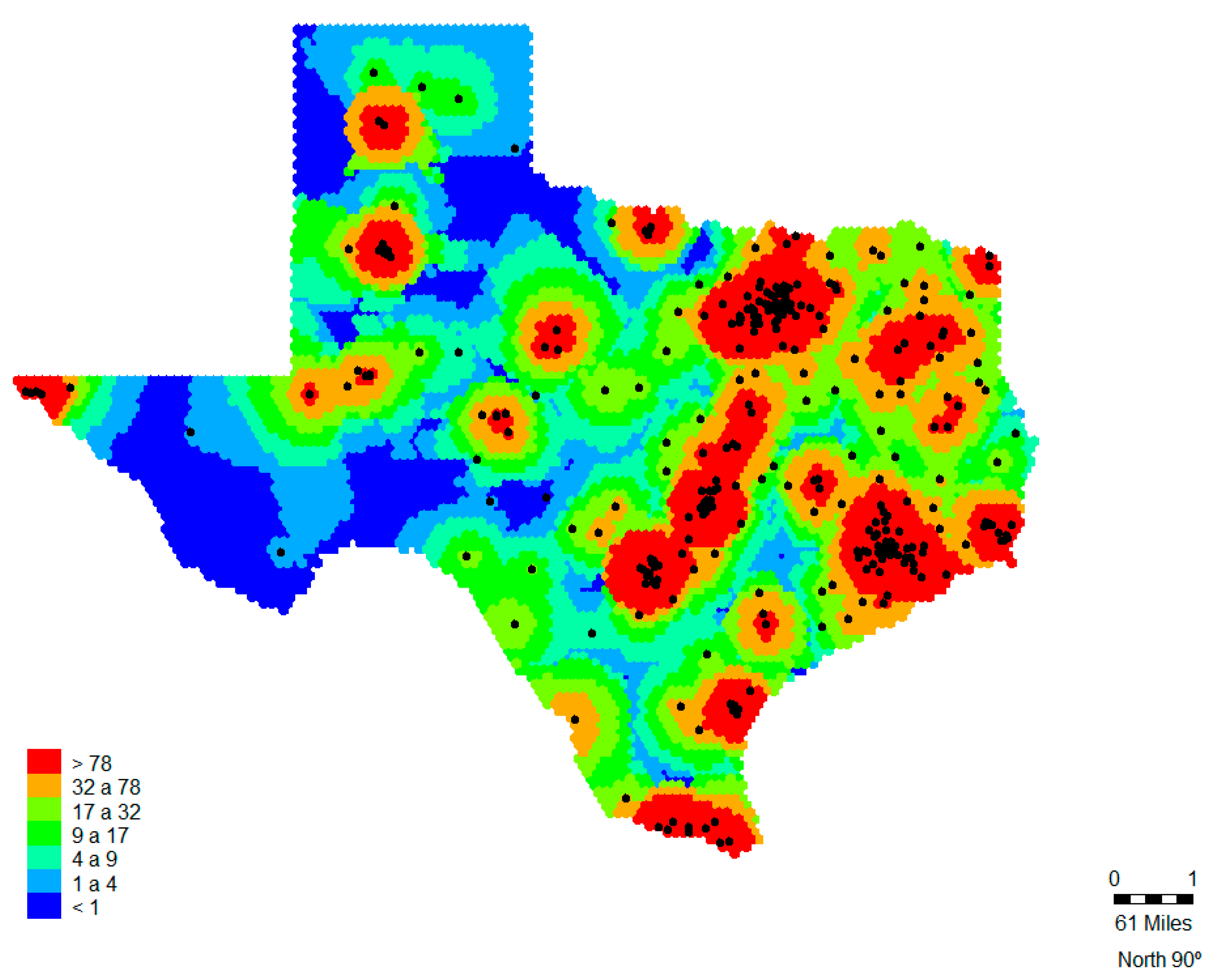
The dependent variable is healthcare accessibility across Texas, , proxied by data on hospital inpatient discharges that occurred during the year 2015. Hospital inpatient discharges is often used as a measure of healthcare use [44]. In order to analyze and visualize the spatial distribution of , the kernel density estimation of the spatial variation of healthcare accessibility was estimated using hospital discharges per 1000 citizens in Texas using Equation (10) as the spatial weighting function (see Figure 1). The kernel density estimation of healthcare accessibility was given by:
where is given by Equation (10), hospital inpatient discharges; is the area of the subregion over which the kernel function is evaluated at grid point g, possibly corrected for edge effects; and c is a constant of proportionality. Since the primary concern was to analyze differences in healthcare accessibility, an adaptive bandwidth up to a maximum distance was applied. There are limitations to this spatial analysis, as the relatively arbitrary selection of bandwidth limits both static and adaptive methods. Too large or small a bandwidth poses the risk of over- or under-smoothing the original data, respectively. Following Carlos et al [45] multiple parameters for bandwidth are tested in a sensitivity analysis. Following de Mello-Sampayo [2], 100 miles limit was set on the density calculation if the expected three hospitals data points’ threshold was not reached. This maximum distance was determined by testing a number of distances, as well as choosing a limit based on behavior theory regarding healthcare accessibility [46].
The density map in Figure 1 shows 7608 cells of one tenth square mile size, which comprise 540 hospital tracts. The hospitals’ location (data points) are shown in black crosses. Figure 1 shows that the distribution of hospital discharges exhibits some form of clustering, as opposed to being random. This result was corroborated by the Moran’s I and Geary’s C (see Table 1). Areas with low values would correspond to areas of relatively poor access and the high point values would indicate areas of potential over-service. The area of highest density are the neighborhoods of the five big cities in Texas: Houston, San Antonio, Dallas, Austin and Fort Worth. Areas of relatively poor accessibility (green areas) include a pocket in the west, next to El Paso, and a considerable number of counties in central Texas and from south of Texas up to the north. The area with the poorest access to health is the corridor from the southwest through the west of Texas and east of the Panhandle (around Carson State). These blue areas are composed mainly of rural counties.
According to the theoretical model proposed in this manuscript, the effects on healthcare accessibility of some specific variables are analyzed. To characterize the healthcare demand market, we used income per capita to control for the socio-economic level of the patients, and low birth weight to control for health level of the patients. The variable income per capita was measured as the after-tax income per capita available on average to individuals living in a given county. In our spatial interaction modeling, average income per capita was likely to capture broadly defined socio-economic factors characterizing demand in each county. Since people in low income or poverty levels are associated with low levels of health [29,47,48,49], a positive relationship between counties’ income per capita and healthcare accessibility is expected to occur. Accordingly, ceteris paribus, better access to healthcare in richer counties is to be observed and therefore there is an emergent pattern of healthcare accessibility. In the literature on hospital choice, income is shown to positively affect spatial accessibility, as richer individuals are able to choose doctors and hospitals to suit time and place, which is not possible for low income patients [50,51]. Low Birth Weight (LBW) is included in this analysis, because of the growing emphasis and interest in measuring and comparing health levels when analyzing healthcare accessibility. Low birth weight is a valuable public health indicator of maternal health, nutrition, healthcare delivery, and poverty [52,53]. The low birth weight rate at the population level is an indicator of a public health problem that includes long-term maternal malnutrition, ill health and poor health care [54]. In this study, this variable proxies health status and well-being of the population accessing healthcare services. Since a higher level of LBW indicates a low health level, it is expected, ceteris paribus, for there to be an inverse relationship between healthcare accessibility and LBW.
The focus was also on analyzing the effects on healthcare accessibility of hospital specific characteristics. The regressor included in our specification is a proxy capturing the broad concept of hospital capacity. The service capacity of hospital is usually proxied by the provider-to-population ratio, defined as the ratio of health service capacity in the numerator (e.g., as the number of physicians or the number of hospital beds) and population size in the denominator. Provider-to-population ratios have often been used in studies linking the supply of healthcare services to health outcomes [55]. Shi and Starfield [56] focused on the effects of primary care physician supply, measured by the population-to-provider ratio, on mortality among Blacks and Whites across U.S. metropolitan areas in 1990. Provider-to-population ratios also take on a pivotal role in the delineation of Health Professional Shortage Areas (HPSAs) and Medically Underserved Areas (MUA) [57,58]. In this study inpatient beds density, defined as number of hospital beds per population density, was used to proxy hospital service capacity [59]. All other things being equal, hospital service capacity is expected to have a positive effect on healthcare accessibility.
3.3. Empirical Strategy
The estimation of standard form of the spatial accessibility pattern as presented in Equation (8) has the problem of the delineation of the bounded areas, and . First, the delineation of the bounded region strongly influences the results, as any change in the area definition will change the measures used to proxy healthcare demand market’s characteristics: patients’ socio-economic level, and patients’ health level. Second, these measures are potentially misleading, since they ignore internal variations of spatial accessibility, especially differences between rural and urban areas.
One way to address the above-mentioned issues is to estimate Equation (8) from numerous points in a region. This study used spatial autoregressive regression (SAR), spatial error regression (SER), geographically weighted regression (GWR) and multilevel modeling (MLM) to evaluate the spatial distribution of existing hospital discharges and their social and economic correlates. These econometric techniques allow using Equation (10) as the spatial accessibility measure. Although the parameter estimates are not directly comparable, the GWR models were fit as a point of reference when evaluating the realism of spatial lag models and establishing the appropriateness and utility of the MLMs.
First, a baseline ordinary least squares (OLS) model was estimated in order to test the adequacy of the spatial econometric techniques used in this empirical application, see the OLS column in Table 2, as follows:
where is the dependent variable: healthcare service accessed by residents’ point at hospital , is the intercept; is the matrix of the independent variables comprising income per capita, low birth weight and hospital service capacity; is the vector of estimated parameters; is the error term assumed i.i.d. Standardized variables, i.e., the grand mean centered variables, are used because the ultimate research question involves the effects of these variables on the healthcare accessibility in Texas’ counties. Evaluating the mean centered variables is especially important for MLM [60,61].
3.3.1. Spatial Econometric Models
Spatial regression models relax the assumption of spatial independence and adjust for spatially autocorrelated processes by incorporating local relationships in the error covariance structure [3,20,21]. All variables exhibited significant spatial autocorrelation, see Moran’s I and Geary’s C statistics shown in Table 1. To control for spatial dependence, SAR and SER models were estimated (see the SAR and SER columns in Table 2). In the spatial lag model (SAR), spatial dependence was modeled as a spatially lagged regressor that is correlated with the error term, and the least squares estimation turned out to be biased and inconsistent due to the simultaneity bias [3]. The SAR model estimated is as follows:
where λ is the spatial dependence parameter and is a spatial link matrix with zero diagonal elements whose non-zero elements express the degree of potential spatial interaction between each possible pair of locations. The spatial-weighting matrix, W, was employed to compute weighted averages in which more weight is placed on nearby observations than on distant observations and parameterize Tobler’s law of geography “Everything is related to everything else, but near things are more related than distant things” [62]. The weights used are the opportunity cost of healthcare accessibility proxied by the spatial accessibility measure given by Equation (10).
In the spatial error model (SER), spatial dependence was modeled as a spatial autoregressive process in the error term. Ignoring spatial dependence in the error term does not yield biased least squares estimates, although their variance will be biased, thereby resulting in misleading inferences [3,20]. The SER model was estimated, see the SER column in Table 2, as follows:
where is the spatial error parameter. Although these models consider the spatiality of the data, they implicitly assume spatial homogeneity. In other words, the spatial models fit global spatial effects but ignore local variation, and do not allow for the possibility of spatial non-stationarity. The kernel density estimation of the healthcare accessibility shown in Figure 1 indicates clusters as opposed to random distribution. Detection of non-stationarity using the GWR models would cast doubt on the reliability of the spatial models’ results.
3.3.2. Geographically Weighted Regression (GWR)
The GWR model was estimated to check for local variations [5,6]. In Equation (12), is the local estimated intercept, and represents the slope of the grand mean-centered kth variable at location j. (see the GWR column in Table 2).
where represents the coordinate location of the data point j, in our case, hospitals. Each observation is weighted according to its proximity to j. The weights used are the opportunity cost of healthcare accessibility proxied by the spatial accessibility measure given by Equation (10).
Some of the local spatial variability may result from sampling variation. The computationally intensive Monte Carlo method, which tests if the observed variation in a parameter is sufficient to reject the null hypothesis of a globally fixed parameter, was carried out. When no real spatial pattern in the parameter exists, any permutation of the regression variables against their locations should be equally likely, providing a model for the null distribution of the variance. Using the Monte Carlo approach, the geographical coordinates of the observations were randomly permuted against the variables a certain number of times. This produces n values of the variance of the coefficient of interest, which are used as an experimental distribution. By comparing the actual variance against this distribution, an experimental significance level was obtained for the spatial variability of each individual parameter.
3.3.3. Multilevel Modeling (MLM)
The MLM both controls for spatial autocorrelation (like the spatial models) and also allows local variation and spatial non-stationarity (like GWR). The MLM combines two-level equations, see Hox (2002). Equation (13) shows the combined random intercept, random slope, two-level model,
where is the county level random effect with its own residual term which is is the hospital scale residual which is is the vector of q coefficients for hospital-level variables; is the vector of coefficients for the c county-level variables; and vector gives the variance of the estimates .
When testing a cross-level interaction model (MLM with interaction), intercepts and slopes were allowed to vary across level-2 units, as follows:
where is the vector of coefficients for the interactions between the level-1 predictor (i.e., hospital service capacity) and the level-2 predictors (i.e., income per capita and low birth weight). To incorporate spatial interaction in the MLMs, we used the spatial-weighting matrix, W, described above for sampling weights at the hospital level.
4. Results
This study used different econometric techniques to evaluate the spatial distribution of healthcare accessibility subject to hospital service capacity, income per capita and low birth weight. Based on an Akaike information criterion (AIC) minimization criterion, the multinomial model (MLM) shown in Table 3 outperformed the spatial models presented in Table 2. The MLM is the model that best fits the data because first the data is found to be spatially non-stationary, making the parameters of the global models difficult to interpret. Secondly, local spatial models allow for potential variations in relationships over space, leading to greater insights into the data generating processes.
The Moran’s I and Geary’s C values calculated from the residuals of the OLS model were positive and significant, thus indicating that the OLS model suffered from spatial autocorrelation. The SAR and SER models outperformed their OLS counterparts, as shown by the Robust Lagrange Multiplier (LM) test [63]. All Alfa coefficients in the spatial models were significant. The spatial lag term (Lambda) was positive and significant, corroborating the strength of the spatial interaction observed in Figure 1. Recalling the endogenous effects discussed in Section 2, a positive and significant value for might indicate the existence of mimicking behavior among neighboring hospitals. This implies that regions with high healthcare accessibility favor the healthcare accessibility of surrounding regions. The spatial error term, ρ (Rho) comprises the indirect effect on healthcare spending of unobserved variables. Rho was negative but weakly significant and lower than most explanatory variables in absolute value, suggesting a low probability of omitted variable bias.
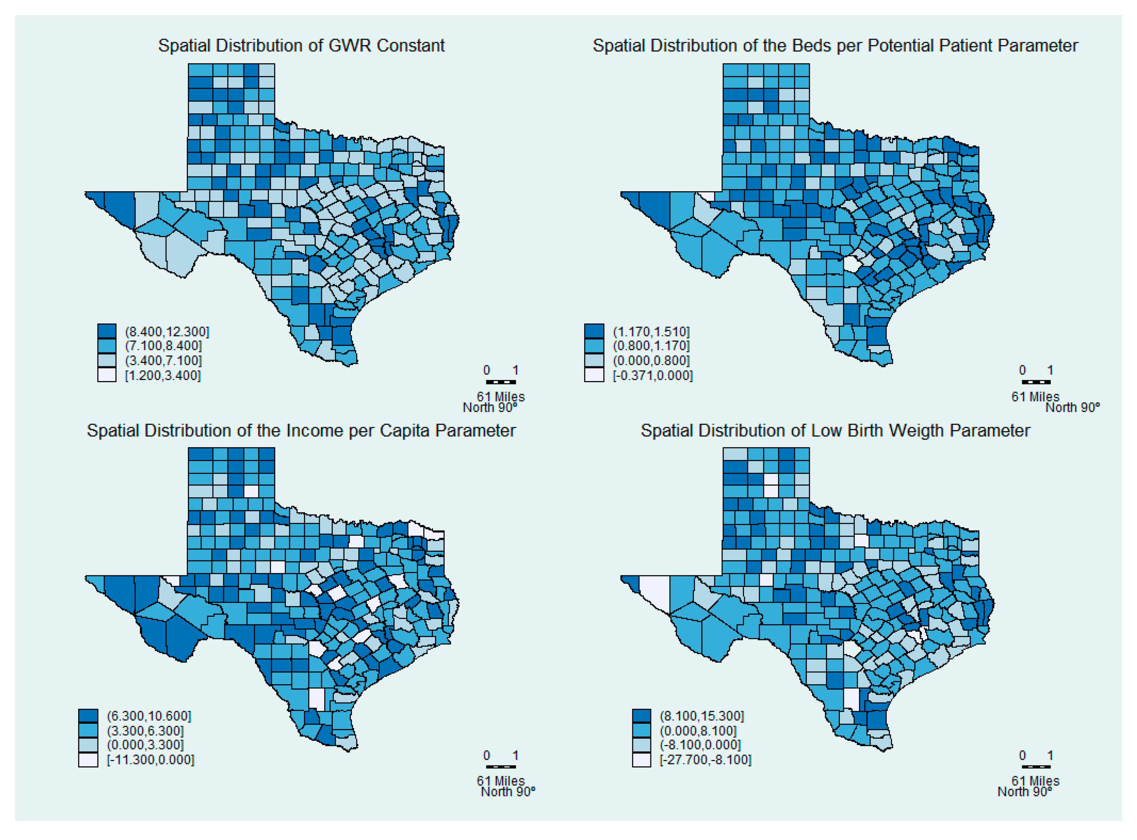
The mean, minimum and maximum GWR coefficients are shown in Table 2. As shown in Figure 2 the spatial distribution of the parameters indicates the degree of spatial non-stationarity and illustrates the interesting way in which the effects vary over space. The Monte Carlo test of significance for the spatial variation in these estimates indicates that the spatial variation is significant. The global SAR and SER models masked the local relationships between the dependent variables and the correlates. The hospital service capacity’s parameter is negative in some counties of Texas, albeit only marginally (0.4%). The spatial variation in the income per capita parameter depicts the differing effect of income per capita across Texas. It had a negative effect in 8.1% of the counties. Contrary to the global models, the mean of the low birth weight parameter is positive, while remaining negative in 30% of local models. In 70% of the counties, low health level patients had good healthcare accessibility.
In Table 3, the intraclass correlation (ICC) shows that 50% of the healthcare accessibility variance occurred across counties. This ICC value is consistent with research [60] that has shown ICC values common in cross-sectional MLM applications in social research studies. However, a non-zero ICC estimate alone does not necessarily indicate the need for multilevel analyses. The design effect quantifies the effect of independence violations on standard error estimates and is an estimate of the multiplier that needs to be applied to standard errors to correct for the negative bias that results from nested data. Design effect estimates greater than 2.0 indicate a need for MLM [60]. The design effect in our study of 3.21 indicates the need for multilevel modeling.
Based on an Akaike information criterion (AIC) minimization criterion, the MLM that included spatial interaction outperformed the others, suggesting that failure to account for patients’ heterogeneity in the trade-off of health and wealth when accessing healthcare may lead to self-selection bias in estimates of spatial healthcare accessibility. The parameter estimates in the MLM models had the same direction as the spatial models. Results of the spatial MLM with interaction show that hospital service capacity had a positive and significant impact on healthcare accessibility (). Low birth weight had a negative and significant relationship () with healthcare accessibility. Interestingly, when interacting with low birth weight, hospital service capacity yields a negative impact (). However, this coefficient is poorly significant, indicating that this effect is absent or weak. Thus, patients with low level of health (or high low-birth weight) in good hospital service capacity areas may access fewer healthcare services.
Results also show that high income patients had significantly higher healthcare accessibility () and higher healthcare accessibility per increase in hospital service capacity (). This important interaction would have gone undetected if only global models were used for the analysis.
Differences in results between SAR, SER and GWR models, as well as MLM show more complex relationships between healthcare accessibility and hospital service capacity, income per capita, and low birth weight. The use of local specifications (GWR) and cross-level (MLM) models uncovered additional complexity that the global models (SAR and SER) were unable to detect.
Discussion
The distribution of healthcare accessibility in Texas was analyzed, with respect to the patients’ socio-economic levels and their health levels. The hospital service capacity was also used to analyze the supply side of the healthcare accessibility. Different spatial econometric techniques were used (SAR, SER, GWR and MLM) to account for the spatial heterogeneity and dependence on healthcare accessibility. Results indicated that the model that accounted for local heterogeneity of healthcare accessibility outperformed all other models. Hence, failure to account for patients’ heterogeneity in the trade-off of health and wealth may lead to self-selection bias in estimates of spatial healthcare accessibility. This study adds to the growing body of literature that highlights the association between the distribution of healthcare facilities or hospitals and the socio-economic characteristics and health level of neighborhood residents [30,31,37,50,64].
The substantial spatial non-stationarity exposed by the GWR and the cross-level MLMs is important to consider. While the non-stationarity of healthcare accessibility in Texas was considered in light of earlier studies [2,65], our local and cross-level interaction models cast some doubt on findings from previous studies using global models [19,30,66]. The generalizability coefficient’s sign and direction from one county to another would seem to be limited if the local sign and direction were opposite in different counties of the same state.
The local GWR and MLM analyses may shed some light on the reasons for the mixed results of previous research that has examined spatial healthcare accessibility. Global models used in previous work found that income was positively associated with access to healthcare [30,31]. Our model showed a non-stationary relationship that ranged from negative to positive depending on the region. The MLM interaction terms indicate a positive association between income per capita with hospital service capacity, which may support the belief that high income level patients have good access to healthcare but have even better access in urban areas [9,42].
Cross-level interaction terms in the MLMs further exposed important sources of variation to consider for future research. As expected, low birth weight at the county level was negatively associated with healthcare accessibility. However, low birth weight interacts with hospital service capacity at the hospital level to produce a coefficient with the same sign (Table 3). The MLM model therefore suggests that in low health level counties with high service capacity, there is relatively low healthcare accessibility. In urban counties, low health level patients might access fewer healthcare facilities. The empirical results provided by local (GWR) and cross-level (MLM) techniques presented here offer a basis for additional theorization as to the explanations regarding healthcare accessibility.
It is important to stress some limitations to our empirical study. First, given that the statistical unit of our analysis is the hospital and county, we would expect variations within each county. Therefore, subsequent analysis would benefit from more disaggregated data at the patient level. Moreover, income per capita was used to proxy socioeconomic status and low birth weight was used for patients’ latent health status. These proxies are limited to describing the demand for healthcare. Future work should be directed to incorporate other measures of demand and supply of healthcare in order to enhance the explanatory power and further policy recommendations of the model.
Straight-line or Euclidian distance, which is the basis for our spatial interaction models, is by far the most popular proxy for travel friction in the health services literature, because it is easily computed from geo-coded locations. However, Euclidian distance may be an imperfect proxy for travel friction. Travel time and travel distance might be better, but these must be computed from transportation network data, a burdensome process that brings in its own sources of error. Some authors use Euclidian distance and travel distance [38,57,58], while others favor time or travel distance over Euclidian distance [39]. This discussion identifies several avenues for methodological improvement: the search for a satisfactory adjustment for demand in health service availability, an adjustment for travel mode options, assessment of the improvements achievable through use of travel time or travel distance and the collection and incorporation of data on mid-level and safety net providers.
It would also be worthwhile to conduct research to determine the most appropriate service radius to use in the creation of provider density layers. This would ideally be the distance beyond which patients find it difficult to maintain a consistent relationship with the provider. A representative survey of city residents and an examination of medical records, indicating patient origin, adequacy of utilization and consistency of patient-provider relationship, could reveal a better radius. Also, given that burden of transportation probably varies with socioeconomic status and neighborhood characteristics, it might be that the radius should vary with ecological circumstances.
5. Conclusions
This paper demonstrates the utility of incorporating the theoretical foundations in spatial interaction models as a tool to assess spatial accessibility to healthcare services, since the data, specification and econometric technique used to estimate the spatial interaction model are affected. Different spatial analytical techniques were applied to examine county-level explanations of the heterogeneity in healthcare accessibility: SAR, SER, GWR and MLM. First, it was found that the local GWR and spatial MLM revealed interesting patterns that were undetected by global models. Second, even when significant relationships were detected using the spatial econometric models, the local GWR detected relationships between income and healthcare accessibility, and between health level and healthcare accessibility that are much more complex and even oppositional. Future research should analyze other factors that may have led to these varied relationships. Finally, the MLM allowed us to uncover interactions between hospital service capacity level and income per capita and health level that were dissimilar to what is indicated in single-level, global analyses.
Funding
Fundação para a Ciência e Tecnologia, under UID/GES/00315/2019 grant is gratefully acknowledged. The funding body had no influence in the design of the study, collection, analysis, or interpretation of data, or in writing the manuscript.
Acknowledgments
Three anonymous reviewers read the manuscript and suggested substantial improvements, and are gratefully acknowledged.
Conflicts of Interest
The author declares no potential conflict of interest.
References
- Moscelli, G.; Siciliani, L.; Gutacker, N.; Cookson, R. Socioeconomic inequality of access to healthcare: Does choice explain the gradient? J. Health Econ. 2018, 57, 290–314. [Google Scholar] [CrossRef] [PubMed]
- de Mello-Sampayo, F. Spatial Interaction Healthcare Accessibility Model—An Application to Texas. Appl. Spat. Anal. Policy 2018, 11, 739–751. [Google Scholar] [CrossRef]
- Anselin, L. Spatial Econometrics: Methods and Models; Kluwer Academic Publishers: Boston, MA, USA, 1988. [Google Scholar]
- Kordi, M.; Fotheringham, A.S. Spatially weighted interaction models (SWIM). Ann. Am. Assoc. Geogr. 2016, 106, 990–1012. [Google Scholar] [CrossRef]
- Fotheringham, A.S.; Brunsdon, C.; Charlton, M. Geographically Weighted Regression: The Analysis of Spatially Varying Relationships; John Wiley & Sons: Hoboken, NJ, USA, 2003. [Google Scholar]
- Fotheringham, A.S.; Charlton, M.E.; Brunsdon, C. Geographically Weighted Regression: A Natural Evolution of the Expansion Method for Spatial Data Analysis. Environ. Plan. A 1998, 30, 1905–1927. [Google Scholar] [CrossRef]
- Subramanian, S.V.; Duncan, C.; Jones, K. Multilevel Perspectives on Modeling Census Data. Environ. Plan. A 2001, 33, 399–417. [Google Scholar] [CrossRef]
- Subramanian, S.V.; Duncan, C.; Jones, K. The Relevance of Multilevel Statistical Methods for Identifying Causal Neighborhood Effects. Soc. Sci. Med. 2004, 58, 1961–1967. [Google Scholar] [CrossRef]
- Shah, T.I.; Bell, S.; Wilson, K. Spatial Accessibility to Health Care Services: Identifying under-Serviced Neighbourhoods in Canadian Urban Areas. PLoS ONE 2016, 11, e0168208. [Google Scholar] [CrossRef]
- Hox, J. Multilevel Modeling: When and Why. In Classification, Data Analysis, and Data Highway; Balderjahn, I., Mathar, R., Schader, M., Eds.; Studies in Classification, Data Analysis, and Knowledge Organization; Springer: Berlin, Heidelberg, 1998; pp. 147–154. [Google Scholar]
- Hox, J. Multilevel Analysis: Techniques and Applications; Erlbaum: Mahwah, NJ, USA, 2002. [Google Scholar]
- Snijders, T.A.B.; Bosker, R.J. Multilevel Analysis: An. Introduction to Basic and Advanced Multilevel Modeling, 2nd ed.; Sage: New York, NY, USA, 2012. [Google Scholar]
- Skinner, J. Causes and consequences of regional variations in health care. In Handbook of Health Economics; Elsevier: North Holland, The Netherlands, 2011; Volume 2, pp. 45–93. [Google Scholar]
- Moscone, F.; Knapp, M.; Tosetti, E. Mental health expenditure in England: A spatial panel approach. J. Health Econ. 2007, 26, 842–864. [Google Scholar] [CrossRef]
- Moscone, F.; Knapp, M. Exploring the spatial dimension of mental health expenditure. J. Ment. Health Policy Econ. 2005, 8, 205–217. [Google Scholar]
- Yu, Y.; Zhang, L.; Li, F.; Zheng, X. Strategic interaction and the determinants of public health expenditures in China: A spatial panel perspective. Ann. Reg. Sci. 2013, 50, 203–221. [Google Scholar] [CrossRef]
- Baltagi, B.; Yen, Y. Hospital treatment rates and spillover effects: Does ownership matter? Reg. Sci. Urban. Econ. 2014, 49, 193–202. [Google Scholar] [CrossRef] [Green Version]
- Gravelle, H.; Santos, R.; Siciliani, L. Does a hospital’s quality depend on the quality of other hospitals? A spatial econometrics approach. Reg. Sci. Urban. Econ. 2014, 49, 203–216. [Google Scholar] [CrossRef] [PubMed] [Green Version]
- Moscone, F.; Skinner, J.; Tosetti, E.; Yasaitis, L. The Association between Medical Care Utilization and Health Outcomes: A Spatial Analysis. Reg. Sci. Urban. Econ. 2019, 77, 306–314. [Google Scholar] [CrossRef]
- Anselin, L. Some robust approaches to testing and estimation in spatial econometrics. Reg. Sci. Urban. Econ. 1990, 20, 141–163. [Google Scholar] [CrossRef]
- Anselin, L.; Florax, R. Small Sample Properties of Tests for Spatial Dependence in Regression Models: Some Further Results. In New directions in spatial econometrics; Anselin, L., Florax, R.J.G.M., Eds.; Springer: Berlin, Germany, 1995; pp. 21–74. [Google Scholar]
- Manski, C. Identification of endogenous social effects: The reflection problem. Rev. Econ. Stud. 1993, 60, 531–542. [Google Scholar] [CrossRef] [Green Version]
- LeSage, J.; Pace, R. Introduction to Spatial Econometrics; Taylor & Francis: Abingdon, UK, 2009. [Google Scholar]
- McMillen, D. Spatial autocorrelation or model misspecification? Int. Reg. Sci. Rev. 1993, 26, 208–217. [Google Scholar] [CrossRef]
- McClellan, M.; McNeil, B.J.; Newhouse, J.P. Does more intensive treatment of acute myocardial infarction in the elderly reduce mortality? Analysis using instrumental variables. JAMA 1994, 272, 859–866. [Google Scholar] [CrossRef]
- Levy, M.; Nir, A.R. The utility of health and wealth. J. Health Econ. 2012, 31, 379–392. [Google Scholar] [CrossRef]
- Finkelstein, A.; Luttmer, E.; Notowidigdo, M. What Good is Wealth Without Health? The Effect of Health on the Marginal Utility of Consumption. J. Eur. Econ. Assoc. 2013, 11, 221–258. [Google Scholar] [CrossRef] [Green Version]
- Chow, J.; Johnson, M.; Austin, M. The Status of Low-Income Neighborhoods in the Post-Welfare Reform Environment: Mapping the Relationship between Poverty and Place. J. Health Soc. Policy 2005, 21, 1–32. [Google Scholar] [CrossRef]
- Braveman, P.; Egerter, S.; Barclay, C. Issue Brief. Series: Exploring the Social Determinants of Health: Income, Wealth and Health; Robert Wood Johnson Foundation: Princeton, NJ, USA, 2011. [Google Scholar]
- Makaroun, L.K.; Brown, R.T.; Diaz-Ramirez, L.G.; Ahalt, C.; Boscardin, W.J.; Lang-Brown, S.; Lee, S. Wealth-Associated Disparities in Death and Disability in the United States and England. JAMA Intern. Med. 2017, 177, 1745–1753. [Google Scholar] [CrossRef]
- Lippi Bruni, M.; Mammi, I. Spatial effects in hospital expenditures: A district level analysis. Health Econ. 2017, 26, 63–77. [Google Scholar] [CrossRef] [PubMed] [Green Version]
- Manski, C. The structure of random utility models. Theory Decis. 1977, 8, 229–254. [Google Scholar] [CrossRef]
- McFadden, D. Modelling the Choice of Residential Location. In Spatial Interaction Theory and Planning Models; Karlqvist, A., Lundqvist, L., Snickars, F., Weibull, J., Eds.; North-Holland: Amsterdam, The Netherlands, 1978; pp. 75–96. [Google Scholar]
- McFadden, D. Econometric Models of Probabilistic Choice; Manski, C., McFadden, D., Eds.; The MIT Press: Cambridge, MA, USA, 1981. [Google Scholar]
- Boyce, D.; Williams, H. Forecasting Urban. Travel: Past, Present and Future; Edward Elgar: Cheltenham, UK; Northampton, MA, USA, 2015. [Google Scholar]
- Roy, J.O. Spatial Interaction Modelling, A regional Science Context; Springer: Berlin/Heidelberg, Germany; New York, NY, USA, 2004. [Google Scholar]
- Nesbitt, R.C.; Gabrysch, S.; Laub, A.; Soremekun, S.; Manu, A.; Kirkwood, B.R.; Amenga-Etego, S.; Wiru, K.; Höfle, B.; Grundy, C. Methods to measure potential spatial access to delivery care in low- and middle-income countries: A case study in rural Ghana. Int. J. Health Geogr. 2014, 13, 25. [Google Scholar] [CrossRef] [PubMed] [Green Version]
- Luo, W. Using a GIS-based floating catchment method to assess areas with shortage of physicians. Health Place 2004, 10, 1–11. [Google Scholar] [CrossRef]
- Luo, W.; Wang, F. Measures of spatial accessibility to health care in a GIS environment: Synthesis and a case study in the Chicago region. Environ. Plan. B Plan. Des. 2003, 30, 865–884. [Google Scholar] [CrossRef] [Green Version]
- Wang, F.; Luo, W. Assessing spatial and nonspatial factors for healthcare access: Towards an integrated approach to defining health professional shortage areas. Health Place 2005, 11, 131–146. [Google Scholar] [CrossRef]
- Dejen, A.; Soni, S.; Semaw, F. Spatial accessibility analysis of healthcare service centers in Gamo Gofa Zone, Ethiopia through Geospatial technique. Remote Sens. Appl. Soc. Environ. 2019, 13, 66–473. [Google Scholar] [CrossRef]
- Van Dis, J. Where we live: Health care in rural vs urban America. JAMA 2002, 287, 108. [Google Scholar] [CrossRef]
- Wholey, D.; Feldman, R.; Christianson, J.B.; Engberg, J. Scale and scope economies among health maintenance organizations. J. Health Econ. 1996, 15, 657–684. [Google Scholar] [CrossRef]
- OECD. Hospital Discharge rates (Indicator); OECD: Paris, France, 2019. [Google Scholar]
- Carlos, A.; Shi, X.; Sargent, J.; Tanski, S.; Berke, E. Density estimation and adaptive bandwidths: A primer for public health practitioners. Int. J. Health Geogr. 2010, 9, 1–8. [Google Scholar] [CrossRef] [Green Version]
- Grossman, D.; White, K.; Hopkins, K.; Potter, J. How greater travel distance due to clinic closures reduced access to abortion in Texas. PRC Res. Brief. 2017, 2, 2. [Google Scholar]
- Bassuk, E.L.; Buckner, J.C.; Perloff, J.N.; Bassuk, S.S. Prevalence of mental health and substance use disorders among homeless and low-income housed mothers. Am. J. Psychiatry 1998, 155, 1561–1564. [Google Scholar] [CrossRef] [PubMed]
- Khullar, D.; Chokshi, D.A. Health, Income, & Poverty: Where We Are & What Could Help. Health Aff. Health Policy Brief. 4 October 2018. [Google Scholar] [CrossRef]
- Srivastava, D.; McGuire, A. Patient access to health care and medicines across low-income countries. Soc. Sci. Med. 2015, 133, 21–27. [Google Scholar] [CrossRef]
- Huang, Y.; Meyer, P.; Jin, L. Neighborhood socioeconomic characteristics, healthcare spatial access, and emergency department visits for ambulatory care sensitive conditions for elderly. Prev. Med. Rep. 2018, 12, 101–105. [Google Scholar] [CrossRef]
- Mosadeghrad, A. Patient choice of a hospital: Implications for health policy and management. Int. J. Health Care Qual. Assur. 2014, 27, 152–164. [Google Scholar] [CrossRef]
- Cutland, C.L.; Lackritz, E.M.; Mallett-Moore, T.; Bardají, A.; Chandrasekaran, R.; Lahariya, C.; Nisar, M.I.; Tapia, M.B.; Pathirana, J.; Kochhar, S.; et al. Low birth weight: Case definition & guidelines for data collection, analysis, and presentation of maternal immunization safety data. Vaccine 2017, 35, 6492–6500. [Google Scholar] [CrossRef]
- Johnson, C.; Jones, S.; Paranjothy, S. Reducing low birth weight: Prioritizing action to address modifiable risk factors. J. Public Health 2017, 39, 122–131. [Google Scholar] [CrossRef] [Green Version]
- Blanc, A.; Wardlaw, T. Monitoring low birth weight: An evaluation of international estimates and an updated estimation procedure. Bull. World Health Organ. 2005, 83, 178–185. [Google Scholar]
- Waldorf, B.; Chen, S.; Unal, E. A Spatial Analysis of Health Care Accessibility and Health Outcomes in Indiana; Spatial Econometrics Association: Cambridge, UK, 2007. [Google Scholar]
- Shi, L.; Starfield, B. The effect of primary care physician supply and income inequality on mortality among blacks and whites in US metropolitan areas. Am. J. Public Health 2001, 91, 1246–1250. [Google Scholar] [CrossRef]
- Guagliardo, M.F. Spatial accessibility of primary care: Concepts, methods and challenges. Int. J. Health Geogr. 2004, 3, 1–13. [Google Scholar] [CrossRef] [PubMed] [Green Version]
- Guagliardo, M.F.; Ronzio, C.R.; Cheung, I.; Chacko, E.; Joseph, J.G. Physician accessibility: An urban case study of pediatric providers. Health Place 2004, 10, 273–283. [Google Scholar] [CrossRef] [PubMed]
- WHO. Global Reference List of 100 Core Health Indicators; WHO: Geneva, Switzerland, 2015. [Google Scholar]
- Peugh, J. A practical guide to multilevel modeling. J. Sch. Psychol. 2010, 48, 85–112. [Google Scholar] [CrossRef] [PubMed]
- Aguinis, H.; Gottfredson, R.K.; Culpepper, S. BestPractice Recommendations for Estimating Cross-Level Interaction Effects Using Multilevel Modeling. J. Manag. 2013, 39, 1490–1528. [Google Scholar]
- Tobler, W. A computer movie simulating urban growth in the Detroit region. Econ. Geogr. 1970, 47, 234–240. [Google Scholar] [CrossRef]
- Anselin, L.; Bera, A.; Florax, R.; Yoon, M. Simple diagnostic tests for spatial dependence. Reg. Sci. Urban. Econ. 1996, 26, 77–104. [Google Scholar] [CrossRef]
- Billé, A.; Arbia, G. Spatial limited dependent variable models: A review focused on specification estimation, and health economics applications. J. Econ. Surv. 2019, 33, 1531–1554. [Google Scholar] [CrossRef] [Green Version]
- de Mello-Sampayo, F. Spatial heterogeneity of quality, use and spending on medicare for the Elderly. Geospat. Health 2018, 13, 66–78. [Google Scholar] [CrossRef]
- Baltagi, B.; Moscone, F.; Santos, R. Spatial Health Econometrics. In Health Econometrics vol. 294, 13, Contributions to Economic Analysis; Baltagi, B., Moscone, F., Eds.; Emerald Publishing Limited: West Yorkshire, UK, 2018; pp. 305–326. [Google Scholar]
Figure 1.
Kernel Density Estimation of Hospital Discharges per 1000 Citizens.

Figure 2.
Spatial Distribution of GWR Parameter Estimates.


Table 1.
Descriptive Statistics.
| Mean | Standard Deviation | Maximum | Minimum | Moran’s I (c) | Geary’s C (c) | |
|---|---|---|---|---|---|---|
| Hospital discharges per 1000 Citizens (a) | 5.412 | 7.889 | 55.900 | 0.001 | 0.01 * | 1.122 ** |
| Hospital Beds per Population Density (a) | 0.775 | 1.609 | 21.223 | 0.002 | 0.039 *** | 0.503 *** |
| Income per capita (thousand dollars) (b) | 48.133 | 8.978 | 67.288 | 31.50 | 0.200 *** | 0.691 *** |
| Low Birth Weight per 1000 Citizens (b) | 0.083 | 0.012 | 0.149 | 0.046 | 0.162 *** | 0.615 *** |
* Rejects the null at the 10% level. ** Rejects the null at the 5% level. *** Rejects the null at the 1% level. (a) Data Source: US Census Bureau (www.census.gov/); (b) Data Source: DSHS (www.dshs.texas.gov/) (c) Moran’s I is a measure of global spatial autocorrelation, while Geary’s C is more sensitive to local spatial autocorrelation.
Table 2.
Estimation of Equations (12)–(15).
| OLS | SAR | SER | GWR | |||
|---|---|---|---|---|---|---|
| Equation (12) | Equation (13) | Equation (14) | Equation (15) | |||
| Mean | Min | Max | ||||
| Intercept () | 7.468 *** (0.063) | 7.453 *** (0.075) | 7.986 *** (0.325) | 7.350 +++ | 3.560 | 12.231 |
| Hospital Service Capacity () | 0.555 *** (0.042) | 0.663 *** (0.057) | 0.548 *** (0.042) | 1.040 +++ | −0.371 (0.4%) | 1.511 |
| Income per Capita () | 2.182 *** (0.320) | 2.729 *** (0.405) | 2.141 *** (0.319) | 4.353 +++ | −11.264 (8.1%) | 10.586 |
| Low birth weight () | −1.396 *** (0.454) | −1.494 *** (0.491) | −1.387 *** (0.451) | 2.255 +++ | −27.721 (30%) | 15.260 |
| Spatial Parameters | ||||||
| Lambda () | 0.176 *** (0.056) | |||||
| Rho () | −0.70 (0.043) | |||||
| Test Statistics | ||||||
| Moran’s I | 0.1 *** | 0.332 *** | ||||
| Geary’s C | 0.928 ** | 0.665 *** | ||||
| Bandwidth | 0.834+++ | |||||
| F(3,536) | 59.22 *** | |||||
| Robust LM Test | 119.51 *** | 123.60 *** | ||||
| -2loglikelihood | 1933.6 | 1923.6 | 1930.6 | |||
| AIC | 1941.2 | 1935.6 | 1942.6 | |||
| N | 540 | 540 | 540 | 540 | ||
+++ Rejects the null at the 1% level - Monte Carlo tests of spatial variability in parentheses. These tests indicate the extent to which the variation in coefficients across space is significantly different from a random distribution. ** Rejects the null at the 5% level. *** Rejects the null at the 1% level. Standard Errors in brackets. Data Source: US Census Bureau and DSHS.
Table 3.
Estimation of Equations (16) and (17).
| MLM | Spatial MLM | MLM With Interactions | Spatial MLM With Interactions | |
|---|---|---|---|---|
| Equation (16) | Equation (17) | |||
| Level 1, Hospital Level, 540 Hospitals | ||||
| Intercept () | 6.362 *** (0.157) | 6.567 *** (0.144) | 6.387 *** (0.158) | 6.664 *** (0.165) |
| Hospital Service Capacity () | 1.119 *** (0.040) | 0.999 *** (0.062) | 1.111 *** (0.041) | 0.976 *** (0.050) |
| Level 2, County Level, 256 counties | ||||
| Income per Capita () | 3.721 *** (0.732) | 3.451 *** (0.886) | 3.401 *** (0.769) | 2.850 *** (0.738) |
| Low birth weight () | −2.308 *** (0.718) | −2.109 *** (0.649) | −1.952 *** (0.964) | −1.383 * (0.818) |
| Cross level Interactions | ||||
| Hospital Service Capacity * Income per Capita () | 0.210 (0.923) | 0.451 ** (0.243) | ||
| Hospital Service Capacity * Low birth weight () | −0.170 (0.356) | −0.351 (0.418) | ||
| Variance Components (random effects) | ||||
| Intercept () | 1.034 *** (0.171) | 0.880 *** (0.215) | 1.037 *** (0.169) | 0.857 *** (0.212) |
| Variance Income per Capita () | 2.627** (1.302) | 2.016 *** (0.950) | 2.557 *** (1,013) | 1.930 *** (0.899) |
| Variance Low birth weight () | 2.295 *** (1.001) | 0.001 *** (0.001) | 1.961 (1.492) | 0.000 *** (0.000) |
| Residual () | 1.033 *** (0.036) | 1.038 *** (0.056) | 1.036 *** (0.036) | 1.138 *** (0.054) |
| Wald Test | 773.37 *** | 339.87 *** | 768.50 *** | 464.96 *** |
| -2loglikelihood | 1750.6 | 1178.9 | 1749.3 | 1176.0 |
| AIC | 1766.6 | 1193.1 | 1769.3 | 1192.9 |
| ICC | 0.500 | 0.500 | 0.500 | 0.500 |
| Design Effect | 3.219 | 3.219 | 3.219 | 3.219 |
*** Rejects the null at the 1% level. ** Rejects the null at the 5% level. * Rejects the null at the 10% level. Standard Errors in brackets. Data Source: US Census Bureau and DSHS.
© 2020 by the author. Licensee MDPI, Basel, Switzerland. This article is an open access article distributed under the terms and conditions of the Creative Commons Attribution (CC BY) license (http://creativecommons.org/licenses/by/4.0/).
Share and Cite
MDPI and ACS Style
de Mello-Sampayo, F. Spatial Interaction Model for Healthcare Accessibility: What Scale Has to Do with It. Sustainability 2020, 12, 4324. https://0-doi-org.brum.beds.ac.uk/10.3390/su12104324
AMA Style
de Mello-Sampayo F. Spatial Interaction Model for Healthcare Accessibility: What Scale Has to Do with It. Sustainability. 2020; 12(10):4324. https://0-doi-org.brum.beds.ac.uk/10.3390/su12104324
Chicago/Turabian Stylede Mello-Sampayo, Felipa. 2020. "Spatial Interaction Model for Healthcare Accessibility: What Scale Has to Do with It" Sustainability 12, no. 10: 4324. https://0-doi-org.brum.beds.ac.uk/10.3390/su12104324
Note that from the first issue of 2016, this journal uses article numbers instead of page numbers. See further details here.