Varying Effects of Urban Tree Canopies on Residential Property Values across Neighborhoods

Ted Rogers School of Management, Ryerson University, Toronto, ON M5G 2C3, Canada
Sustainability 2020, 12(10), 4331; https://0-doi-org.brum.beds.ac.uk/10.3390/su12104331
Submission received: 14 April 2020
/
Revised: 13 May 2020
/
Accepted: 20 May 2020
/
Published: 25 May 2020
(This article belongs to the Special Issue Sustainable Real Estate: Management, Assessment and Innovations)
Abstract
:As more land area than ever is covered with impermeable surfaces causing problems in the environment, urban trees are effective not only in mitigating environmental problems in the built environment and reducing buildings’ energy use, but also in increasing social and economic benefits. However, the benefits urban trees provide are not evenly distributed but rather disproportionately distributed in high-income neighborhoods. The purpose of this study is to estimate the varying effects of urban trees based on a variety of factors that have influence on tree canopy coverage, including land constraints, new developments, financial capacity to maintain trees, and neighborhood characteristics. Using a unique dataset that includes 24,203 single-family residential sales from 2007 to 2015 merged with Urban Tree Canopy (UTC), this study utilizes spatial models to empirically evaluate the impact of UTC on residential property values in the housing market. Multi-Level Mixed (MLM) models are used to capture the varying effects of tree cover, based on land constraints, new development, financial capacity, and neighborhood characteristics. The findings show the effect of trees is positive and varies across neighborhoods, and implication of the results to best achieve specific desired outcomes in tree-related policies and urban development are apparent.
1. Introduction
Demand for real estate developments of residential, commercial and other uses has led to urbanization and urban sprawl, resulting in significant impacts on environmental degradation. Due to land constrains for development in the built environment, most of the new developments are likely concentrated at urban fringes. According to Alig et al. [1], the increase in developed land has come from the conversion of adjacent forestland. As more land is covered with impermeable surfaces, such as streets, sidewalks, driveways, and building rooftops, the incidence and severity of serious environmental problems, such as urban heat islands, storm-water runoff, and flooding are increased [2].
Trees are effective in mitigating the environmental problems in the built environment and reducing buildings’ energy use [3]. Trees can also provide attractive scenery as well as an acoustic screen between traffic noise and residential areas [4]. Trees also beautify neighborhoods and enhance residents’ well-being [5], as well as increase economic opportunities through increasing sales in retail and commercial business by providing a favorable impression to shoppers, water savings and green jobs [6]. However, according to Schwarz et al. [7], maintaining tree cover creates potential costs and burdens, including the price of water supply in a changing climate, socio-demographic preferences and characteristics, and fiscal capacity to maintain tree cover. As a result, the benefits of tree canopies are unevenly distributed and disproportionally concentrated in high-income neighborhoods [7]. Ethnic/racial minorities and lower-income neighborhoods who have been traditionally marginalized lack the resources or capacity to overcome a scarcity of environmental benefits.
Motivated by the work of Schwarz et al. [7], this study attempts to examine the varying effects of tree cover of individual dwellings in the urban area on the residential property value across neighborhoods. Measuring these advantages of tree cover is challenging since many factors should be considered, such as residents’ demographic characteristics costs incurred. The spatial distribution of land for development and for green space should be determined by residential choice [8] and, therefore, whether land is conserved or developed could be justified based on the economic value of tree canopies on house prices [9]. Of particular interest to this study are the varying effects of tree coverage across neighborhoods, based on a variety of factors affecting the size and proportion of tree canopy coverage, including land constraints, new developments, financial capacity to maintain trees, and neighborhood characteristics. Using a data set of 24,203 single-family residential sales from 2007 to 2015 in Des Moines, Iowa, two analytical approaches are used: a spatial model to control for spatial autocorrelation and a Multi-Level Mixed model (MLM) to estimate the varying effects of tree canopies based on the aforementioned factors.
The findings from this study indicate that there is a positive effect of tree coverage on housing prices, on average, which is consistent with previous research [10]. Moreover, the findings confirm the varying effects of tree canopies across the neighborhoods. The positive effect of tree canopies was found for homes with large lots, particularly in high-income neighborhoods, while tree canopies have a negative effect on the house value in low income neighborhoods, implying that the varying effects of tree canopies across neighborhoods mainly result from different financial abilities to maintain trees (Schwarz et al. 2015) [7]. Since the varying effects of an Urban Tree Canopy (UTC) may result in uneven distribution of tree canopies and disproportional concentration in particular neighborhoods, examining price variability between neighborhoods and measuring the varying effects of UTC play a vital role in policy decisions. Implication of the results to best achieve specific desired outcomes in tree-related policies and urban development are apparent.
This study extends the literature in two ways. First, this study estimates the varying effects of the tree canopies on the residential property using an advanced technical approach. These results suggest that the housing price differentials due to the tree canopy variation may be an additional characteristic to be included in the hedonic price model framework. The multi-level model allows for spatial heterogeneity in estimating tree-related housing price differentials in each neighborhood. Second, the findings of the varying effects of tree canopy coverages also shed light on how to implement the tree-related program to best achieve specific desired planning and urban development outcomes. The remainder of the paper is organized as follows: Section 2 provides a review of existing literature. Section 3 discusses the data and presents the empirical strategy, Section 4 presents the findings, and Section 5 concludes.
2. Related Literature
This section starts with the definition of tree canopies, then discusses methodologies for measuring tree canopy coverages, and finally describes the studies that estimate the benefits of trees on house prices. Previous literature has found that trees are positively correlated with residential property values. However, only a few studies have examined the varying effects of tree coverage (see Greene et al. [11]).
An Urban Tree Canopy, or UTC, is defined either as the size (or percentage) of the tree canopy relative to the total land area [12], or simply as the number of trees [13,14]. A field survey [14] and photographs [13] have been used to count the number of trees and gather extensive information, such as tree species, tree sizes, and environmental and landscape attributes. For instance, Anderson and Cordell [13] counted the number of trees, noting species and size, by looking at manually recorded written descriptions of properties from a Multi Listing Service (MLS) and black and white photographs. They found a positive correlation between the number of trees and housing prices. In particular, intermediate and large trees increased housing prices by $2750 on average. François et al. [14] collected extensive information on environmental and landscape attributes from a combination of CAD (Computer Aided Design), GIS (Geographic Information System) and field surveys. They found that, in general, an additional 1% of tree cover increases housing prices by 0.2%, and what they termed the “scarcity premium” differs depending on demographics, housing types, types of vegetation, and visibility.
Recent studies have begun to use aerial photos and high-resolution remotely-sensed imagery of land cover and impervious surfaces to determine tree canopy [10], since previous methods are effective only for small geographical areas. Sander et al. [10] examined the effect of trees in the Ramsey and Dakota Counties in the Minneapolis Metro area including 39 cities and 14 townships that consist of a mix of urban, suburban, and rural areas. They used the National Land Cover Database (NLCD), which leverages remotely-sensed imagery, to identify tree coverage, and found that a 10% increase in tree cover within 100 m raised the average home price by 0.48% ($1371) and within 205 m, the sale price increased by 0.29% ($836). Aerial photos have been used to identify not only tree coverage but also green covers. Conway et al. [15] defined green cover to include space that has a tree canopy, parkway, lawn, landscaped area, sports field, or cemetery, and determined the amount of cover acreage at each buffer distance of each house. They confirmed the significant positive impact of immediate neighborhood green space and found that increasing green space by 1% within 200 to 300 feet of a property increases the property value by 0.07% in Los Angeles, CA, USA.
The benefits attributed to urban tree canopies, including aesthetics, storm water runoff reduction, carbon dioxide reduction, and air quality improvement are challenging to measure in the monetary values and to translate into economic terms [13]. To estimate the value of public trees, such as city trees and street trees, Maco and McPherson [16] conduct a benefit-to-cost analysis of investing in city trees in Davis, California, and found the benefits to outweigh the costs, at a ratio of 3.8 to 1. However, the benefits associated with tress in individual dwellings, including beautification, shade, privacy, noise abatement, wind reduction, and soil protection, depend on buyer willingness to pay for tree canopies in housing prices. The majority of studies on examining the effect of trees found that the willingness to pay for trees is positively correlated with housing prices.
To measure the willingness to pay, among models used, the hedonic model estimated with Ordinary Least Squares (OLS) is the most frequently used statistical tool for analyzing the impact of a UTC on nearby property values and rental rates. In general, the environmental benefits associated with urban forests, including cleaning and improving air quality [17,18,19], are positively correlated with housing prices, while air pollution has a negative impact [20]. Laverne and Winson-Geideman [21], for instance, examined various attributes of landscape, including visual screening, noise attenuation, shade to parking areas, shade to buildings, recreational enhancement, space definition, and aesthetics on office rental rates. Among these attributes, good aesthetics and good building shade increased rental rates by about 7%, while others had no or negative effect. However, Cho et al. [22] addressed the limitations of the hedonic price model: “hedonic models estimated by OLS cannot be complete without consideration of the spatial configuration of green open spaces within a neighborhood” [22] (p. 415). In addition, Cho et al. [22] argued that the value of open space is sensitive to lot size, and the value of lot size increases as the distance to open space increases, which implies that site-specific land use management is needed because of spatial variation in amenity values. In order to control for spatial effects, more recent studies have started to use advanced statistical methods, such as spatial models [15,22,23], geographically weighted regression models [24], and multi-level hedonic models [25]. A variety of land covers, such as irrigated grass, non-irrigated grass or bare soil, and tree canopy, were examined using the Cliff–Ord model with fixed effects and a geographically weighted model in [24].
To investigate the causal effect of tree planting on housing prices, Wachter and Wong [26] used a difference-in-difference model to examine two tree planting programs; the Philadelphia Horticulture Society (PHS) program focused on low-income neighborhoods and the individual-based Fairmount Park Commission program. They found a significant housing price premium due to an individual local resident tree planting program. The house price differential for parcels sold within 1000 feet of tree planting was between 7% and 11%, of which 2% was attributed to the intrinsic value of trees, another 2% to omitted variable bias, and the remainder to a signaling effect. This signaling effect has high economic significance and is related to the degree of coercion among neighbors and details of the housing condition. The study was very limited, as 1151 tree plantings impacted 0.14% of sales (measured within 100 ft) and 2.15% of sales (measured within 1000 ft) were used.
That being said, the distribution of urban tree cover is uneven and inequitable, in that tree cover is highly associated with income. Schwarz et al. [7] examined the relationship between UTC and demographics, including race/ethnicity and household income, in seven cities across the US: Baltimore, MD; Los Angeles, CA; New York, NY; Philadelphia, PA; Raleigh, NC; Sacramento, CA; and Washington, DC. They found that the effect of tree cover varies across the cities as well as neighborhoods with income, a factor positively and significantly correlated with UTC across all cities examined. They concluded that UTC is disproportionately distributed in high-income neighborhoods because some traditionally disadvantaged and marginalized neighborhoods have a lack of resources or capacity to overcome a scarcity of environmental benefits. UTC could be viewed as a disamenty because it entails increased water demand, maintenance costs, allergies, and perceived safety concerns. Therefore, public investment and tree-related plans take the fact that trees indeed grow on money as concluded by Schwarz et al. [7] into consideration.
In summary, this study extends and contributes to the existing literature by estimating the varying effects of private tree coverage on house sales price. To do so, I use advanced methods—spatial and MLM models. It is also noteworthy that tree canopy coverages are defined as not only a percentage of tree coverage for each residential lot but also as the size of tree canopies in an immediate neighborhood. Neighborhood trees would reflect unobserved neighborhood characteristics. As Wachter and Wong [26] note, tree planting is viewed as a proxy of neighborhood social capital and signaling effects include details of the house condition or the degree of coercion among neighbors.
3. Data and Study Area
The city of Des Moines, located in Polk County, is the capital and largest city in Iowa. The city houses several headquarters of insurance and financial service firms. According to the 2014 US Census, 78% of the total population is white, followed by African American (11%) and Asians (5%). The median household income is $81,239, which is slightly higher than the state and US averages ($67,621 and $74,596, respectively). The city of Des Moines is a typical mid-sized city, with a total of population that has grown from 203,433 in 2010 to 216,853 in 2018. The city of Des Moines provides an ideal setting to test the varying effects of urban trees across neighborhoods with old and new housing stocks as well as different levels of intensification.
Although the city has had steady population increases overall, many of the inner-city neighborhoods have lost population as middle-class households moved to the suburbs. This has resulted in a surplus supply of housing and a house price decline in the inner city. Based on a study to understand the challenges facing the city’s declining neighborhoods and identify techniques for stabilizing and strengthening them, Des Moines encouraged residents to form voluntary neighborhood associations based on geographical proximity. There are 54 neighborhood associations in the city that are generally homogenous in terms of socio-economic status, construction year, and residential property values. In addition, neighborhood tree programs are implemented through a planning process; therefore, the neighborhoods’ participation and their involvement in tree planting and maintenance are critical for the programs’ success [27]. On the other hand, the city has continuously attempted to annex neighboring municipalities and the city boundary has stretched toward the south and east of the city in order to accommodate an increasing population. The city has been experiencing substantial sprawl to meet development demand for residential, commercial, and other real estate uses.
A dataset using parcel-level sales data and UTC was constructed. The housing sales data were obtained from the Polk County Assessor’s Office, and include detailed information on sale price and sale date, as well as structural characteristics, such as the size of the living area, the size of land, bedrooms, bathrooms, construction year, condition of the structure, and presence and type of garage. The initial data contained 40,566 observations from 2007 to 2015, of which 24,203 single-family residential sales were included for the final dataset after removing sales with missing information, sales with a price below $10,000 and non-single family home sales. Since the tree coverage data were collected in 2007 using high-resolution aerial imagery, homes constructed after that date were removed from the dataset. The tree coverage data might not be accurate for new construction, since trees may have been added or removed during the construction process. The average tree coverage was 34.88% and the average housing price was $105,593 during the study period. The detailed variables’ definitions and their descriptive statistics are presented in Table 1.
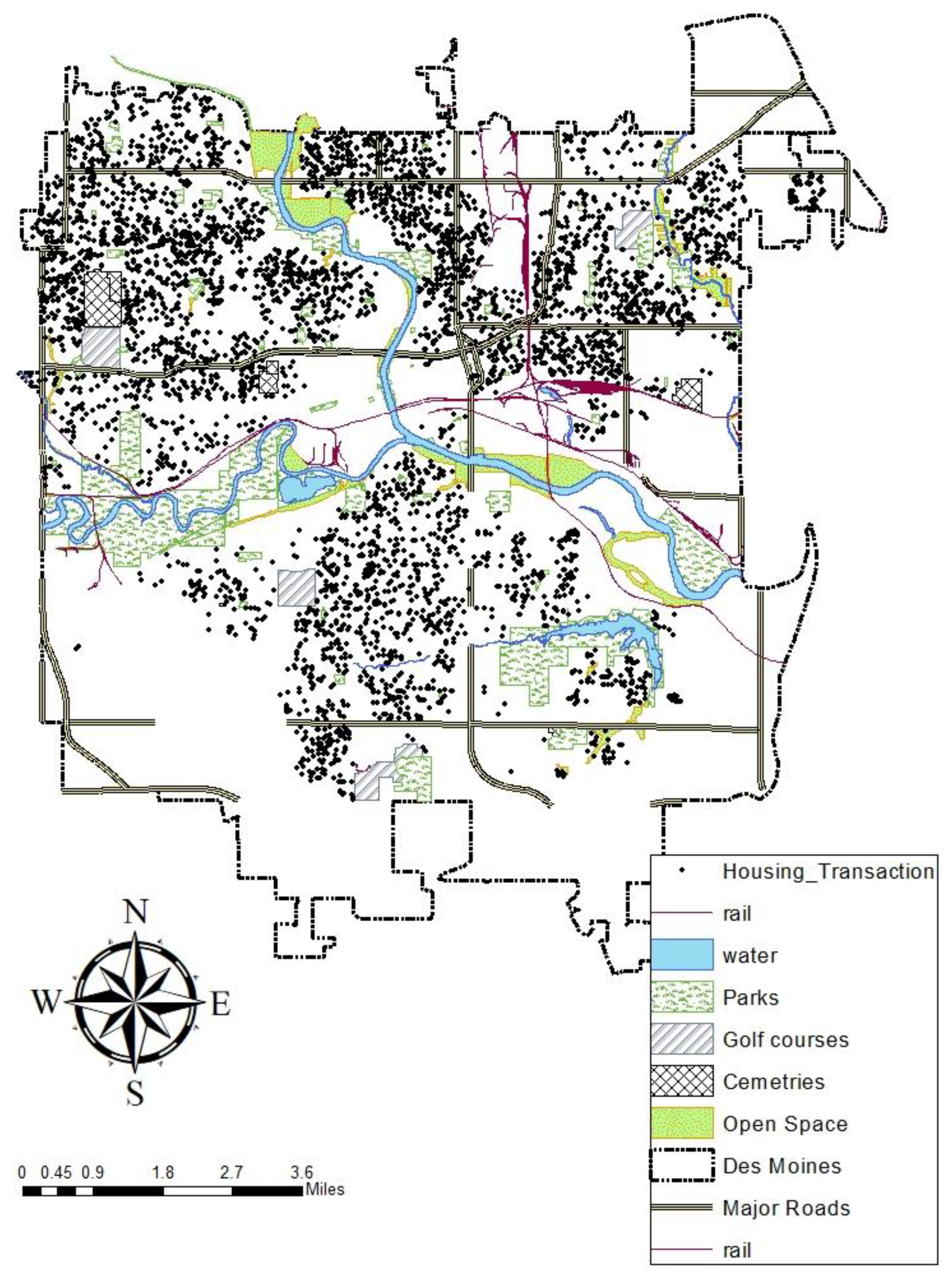
The address information in the sales transaction dataset enables researchers to geocode each sale and to identify the census block-group and neighborhood. Information on neighborhood characteristics including the percentage of white population and household median income were obtained from the US 2010 Census at the census block-group level. Crime rates were obtained from the Areavibes website, which contains a detailed overview of all crimes in Des Moines as reported by the local enforcement agency. Using a standard geographic information system (GIS), location-specific variables were created, including the percentage of tree canopy coverage per parcel and the size of the tree coverage in immediate neighborhoods. I drew 500 feet buffers around major roads and railroads, which are expected to exert a negative effect on residential property values due to the noise nuisance. Lastly, buffers were drawn along the rivers to identify sales within 500 feet. Mixed effects due to both amenities (accessibility and view) and disamenities (noise and traffic) were expected in areas near water. Parks, open spaces, golf courses, and cemeteries were used to control for undeveloped or uncovered land, as shown in Figure 1.
A UTC shape file was obtained from the Spatial Analysis Laboratory (SAL) of the Rubenstein School of the Environment and Natural Resources at the University of Vermont. The SAL measures the coverage of trees based on the 2007 high-resolution aerial imagery and light detection and ranging (LiDAR) data in Des Moines. This project was funded by the USDA (US Department of Agriculture) for UTC assessment protocols to the city of Des Moines. However, the UTC information includes the size of tree coverage but does not provide detailed information on tree species or heights. According to the report [28], 12,466 acres of the city of Des Moines are covered by a tree canopy, accounting for 26% of the total area. The highest percentage of UTC was found on land designated as residential, government, and schools. In addition, the report compares the existing UTC in Des Moines with other cities that have completed similar UTC assessments. The coverage of tree canopy in Des Moines is similar to that of much bigger cities, such as New York, NY (23%) and Boston, MA (29%), but much smaller than comparable-sized cities, such as Greenbelt, MD (62%) and Baltimore County, MD (49%).
At the neighborhood level, tree coverage varies based on several factors, including land constraints, new development, financial capacity, and neighborhood characteristics. The lot size of the land and the age of the structure are used as the proxy variables representing the land constraint, and new development as time constraints for tree growth. I expected the values of tree canopies will increase as the size of land and the age of the structure increase. Anecdotal evidence suggests that trees are more of a burden than a benefit in particularly marginalized neighborhoods with a lack of resources for tree care. The low-income neighborhoods may not be able to afford to plant and maintain trees because trees require regular watering and trimming, and are vulnerable to various diseases. Since income at the individual household level is not available, I used the neighborhood median income as a proxy to represent neighborhood financial capacity to maintain trees, and expected the value of trees will increase as the neighborhood income increases. Lastly, I constructed neighborhood characteristic variables using the combination of the average age of the properties and the average neighborhood income. I categorized neighborhoods into five groups: “old and poor”, “old and affluent”, “new and poor”, “new and affluent” and “mid and med” as a reference. For simplicity, I constructed discrete variables for these factors by partitioning the continuous variables into five categories based on percentiles As seen in Table 2, the %_tree significantly varies across the percentiles of the size of the land, the age of the structure, neighborhood income, and neighborhood characteristics.
The old and affluent neighborhoods in Des Moines have higher tree coverage in their lots than the rest of the city. For example, tree coverage ranges from 65% in Westwood to 3% in some newly developed neighborhoods at the city boundary such as Hillsboro. An example of an older neighborhood with low coverage is East Village at 8%, which has a low median income and a location close to downtown. The tree canopy has higher coverage in “old and affluent” (36.38%) and “old and poor” (33.96%) compared to “new and affluent” (34.54%) and “new and poor” (32.89%). One of the potential explanations of low tree coverages in the “old and poor” neighborhoods might be that residents cannot afford to plant trees or to properly maintain them. Newly developed areas generally have lower tree canopy coverage than the old neighborhoods, which may be because construction sites are often cleared of trees to facilitate construction and reduce costs. Replacement trees that may have been planted would still be small and immature in new neighborhoods.
4. Model
To test the hypotheses that the effect of tree cover will vary across neighborhoods with different physical property characteristics and socio-economic characteristics, two approaches were used: a spatial model to control for spatial autocorrelation and a Multi-Level Mixed model (MLM) to estimate the varying effects of tree canopies. As noted earlier, Cho et al. [23] argued that the value of open space is sensitive to lot size, and the value of lot size increases as distance to open space increases, indicating spatial variation in land use. The spatial model is used to resolve such problems as well as unobservable factors, and potential biased coefficients estimated from the traditional hedonic price model because house prices are spatially correlated with neighboring home sales prices that cause a spatial autocorrelation problem. Nevertheless, the spatial model is limited to test the hypothesis that the effect of tree cover varies across neighborhoods. The varying effects of tree coverage on house prices cannot be measured in a single hedonic price model, and each market needs its own model to estimate the varying effects. However, the coefficients estimated from different equations cannot be directly compared due to different sampling distributions. A Multi-Level Mixed model (MLM) including fixed and random effects allows accounting for the varying effects of trees across the neighborhoods.
4.1. Spatial Model
To detect spatial dependence and spatial heterogeneity, the Lagrange Multiplier (LM) tests were used after the OLS model. The LM tests for spatial lag and spatial error and robust lag and robust error. A Portmanteau test for serial correlation was used to determine which model is appropriate [29]. The results suggested the use of a spatial autoregressive lag and error model (SARAR (1,1)) to deal with the spatial autocorrelation and heteroskedastic disturbances. The spatial model will serve as a baseline model and will aid in understanding an average effect of tree coverages on sale prices across the city. I estimated the effect of tree canopies on the residential property value in the traditional hedonic framework. The home sale price is a function of physical and neighborhood characteristics, location, and the size of tree canopies. The model is specified as follows:
where is a vector of the log of sales price of each home home (i) in neighborhood (j) and X is a vector of physical structural and neighborhood characteristics. , the vector of regression error term, is assumed to be normally distributed with mean 0, and vij is a vector of innovations.
The physical structural variables include the age, lot size, the number of bathrooms, the number of bedrooms, fireplace, size of finished basement, categorical variables of property conditions (poor, below poor, normal, good, and above good), and foreclosure status. Floor and Area Ratio (FAR), which is the ratio of the building square footage to the size of land, is used to control for density and is expected to be negative. The neighborhood variables include the percentage of white population and the log of household median income at the block group level. z is the year fixed effect and q is the quarter fixed effect, all of which are the time-fixed effects to control for the unexpected effect and seasonal effect. are vectors of regression coefficients to be estimated.
The variable %_tree, which is the percentage of tree canopy coverage, is the key variable of interest for this analysis. As noted earlier, two measures of the variable %_tree—percentage of tree canopy to the lot size and the log of the tree canopy size—are used. The former reflects the relative size of the tree canopies, while the latter reflects the absolute size of the tree canopies. The coefficient reflects the marginal willingness to pay for additional percentage of trees and is expected to be positive. is a spatial weight matrix created based on the k-nearest distance between each pair of spatial units, i and j. That is, is as follows;
where is a set of distances between each pair of spatial units and , and that contains the k closest units to .
Generalized Method of Moments (GMM) estimates are used in a Generalized Spatial Two-Stage Least Squares Estimator (GS2SLS) for the spatial lag model. Bivand and Piras [30] explain the steps of estimation for the spatial lag model. First, the initial estimator of is obtained using the regression residuals. The sample moment and residual obtained from the first step are transformed into a generalized spatial two-stage least squares model. In the second step, the variance–covariance matrix of the sample moment vector is estimated based on the residuals from the generalized least squares model. The advantages of this method are that the computation is simple for large samples, and more consistent parameters are generated and compared to the maximum likelihood method [31,32]. These spatial models will portray overall housing market conditions in Des Moines and provide the average impact of tree canopies on the residential property value across the city after controlling for spatial effects.
4.2. Multi-Level Model
As noted earlier, it can be argued that the effect of urban tree coverage will differ between densely constructed inner city neighborhoods with less space for trees and suburban neighborhoods with large lots. In addition, newly developed areas may have formerly had agricultural uses, which implies fewer trees. This is particularly true for grassland areas such as Des Moines, IA. Trees removed during the construction process can be replanted, but it takes years to fully grow and replace old and large trees. The MLM model, which allows coefficients to vary, is able to estimate tree-related sales differentials and measure spatial variation in the effect of UTCs.
To incorporate random effects into the model, the model is rewritten and combines Equations (1) and (3) as:
The effect of the tree canopy is decomposed into a fixed effect (γ10) and random effect (). The fixed effect (γ10) is the grand mean that is constant across the neighborhoods, while the random effect () is a deviation from the mean that captures the varying coefficients and different effect of tree coverage for each neighborhood. If there are no varying effects of trees on house prices, equals zero.
5. Model Results
5.1. Spatial Model Results
The results of the LM test suggest that a SARAR (1,1) (the first order spatial autoregressive and disturbances) model is appropriate to control for both spatial autocorrelation and heteroskedastic disturbances. Table 3 reports the results of the five spatial models: (1) the base; and the interactions between (2) %_tree and log of land; (3) %_tree and age; (4) %_tree and log of income; and (5) %_tree and age together with log of income. The OLS model results are presented in the Appendix A. The magnitudes and signs for each variable used in the models were consistent with the expectation. For the physical characteristics, log of the land size, log of living area size, number of bathrooms, and number of bedrooms were positively correlated with house prices, all of which were statistically significant. In particular, the log of living space had a substantial positive effect on house prices with a high t-value. Five categories of the condition variables (good, above normal, normal, below normal, and poor) were used to control for the physical condition of the housing structure. Using the “normal” condition as a reference category, the physical condition variables had positive signs for better quality and negative signs for poorer conditions, all of which were statistically significant with very high t-values and low p-values (p < 0.001). As in most hedonic studies, sales price decreases with age, which is also statistically significant. To control for the density of the development, the variable Floor Area Ratio (FAR) was added in the model and indicated a negative effect on housing prices.
The median income and the percentage of white population at the block-group level were positively correlated with house prices as expected, while the crime rate and foreclosure were negatively correlated with property values. The year and quarter time-fixed effects were also included in the model to control for any unexpected events during the study period. Proximities to rail tracks and major roads exerted negative effects, while proximity to a golf course was positively correlated with housing prices.
Of particular interest in this study is the effect of tree canopy cover (%_tree) on the property values. The effects of %_tree were mixed across the models with and without the interactive variables, implying that %_tree is associated with these factors. More specifically, the base model result indicated that %_tree is positive but is not statistically significant in Model (1). The coefficient of %_tree was 0.006, which can be interpreted as the implicit price of tree cover that can be used to recover marginal willingness to pay. Hence, an additional 1% of tree canopy coverage increases house prices by 0.006% ($633.56 at the average housing price of $105,593), holding all else equal. The interaction variables between %_tree and all the variables including the log of land, age, and the log of income were positive, implying that the effects increase as land size, age, and income increase, all of which are statistically significant.
5.2. Multi-Level Model Results
Panels A and B of Table 4 report the fixed and random model results, respectively. The results of Panel A are similar to those of the spatial models in terms of magnitudes and signs. In particular, Panel B includes the range of the percentiles and the random coefficients estimated by the multi-level models that reveal the varying effects of tree canopies across houses with different land constraints, new construction, neighborhood median incomes, and neighborhood characteristics. As noted earlier, the lot size was used as a proxy for land constraints. The average lot size in Des Moines is 9894 square feet. As expected, the random coefficients for the tree canopy varied based on the land size. The negative effect was found for houses with small lots, and the sign turned positive for those with lots larger than about 6600 square feet. The positive effect increased as the lot size increased. Homes with large lot sizes benefited more from trees, holding others constant.
Similarly, the relationship between the effect of tree canopies on house price and house age was positive. The random model results indicate that there is a negative effect for homes aged 62 years and under, but the signs turned positive for homes aged over 63 years old. As expected, the neighborhood income, which reflects the financial capacity to maintain trees, was also an important factor in determining the size of the tree canopy effect. The tree canopy effect was negative on housing prices in the neighborhoods with income lower than $63,859; then it became positive for those with an income of more than $63,860. The discount for %_tree decreased as income increased.
The effect of tree canopies was also positively correlated with housing prices in the “old and affluent” and “new and affluent” neighborhoods, and negatively correlated in both the “old and poor” and “new and poor” neighborhoods. Counterintuitively, the effect of tree canopies had a positive effect in the “new and affluent” neighborhood, and the magnitude was larger than that of the “old and affluent” group. The results indicate that “new and affluent” neighborhoods with high housing prices of around $137,880 located in the south and north sides of the city have minimal tree canopies (ranging from 3% to 30%), but these neighborhood are more willing to pay a premium for an additional percentage of tree canopy coverage than the other neighborhoods. These model results support the argument of Schwarz et al. [7] that tree coverages are highly correlated with income, since maintaining tree canopy cover is challenging for low-income neighborhoods, in particularly some cities in California with arid weather. These results strongly imply that financial resources may play a critical role in determining tree canopy coverages at the neighborhood level and are the most influential factor for the positive effect of trees on housing prices.
6. Conclusions and Discussions
This study examined the value of tree coverages on single-family residential property sales prices and house price differentials associated with the tree canopy coverages in the city of Des Moines, Iowa. Using 24,513 sales data from 2007 to 2015, the spatial model results indicate that tree canopy coverages are positively correlated with and capitalized into the residential property values. The results are consistent with and confirm previous findings.
The results of the multi-level model support the varying effects of tree coverages and indicate that residents’ willingness to pay for trees differs across the neighborhoods based on land constraints, new development, financial resources, and neighborhood characteristics. The model results also support the argument that tree coverages would be burdens in especially marginalized neighborhoods and imply that it may be due to financial capacity to plant and maintain them, while the positive effect of trees is found for homes with large lots in old, new, and high-income neighborhoods. High-income neighborhoods are more willing to pay for the benefits trees provide, including privacy, accentuated views and so forth, than low-income neighborhoods. The varying effects of trees on house prices across the neighborhoods have important policy implications for city planners when deciding how to implement tree-related policies, and for real estate developers to determine where and how to develop a project.
As noted, if the negative effect of UTCs on sales prices in low-income neighborhoods is the result of a lack of financial resources to overcome a scarcity of environmental benefits, then planting trees in these neighborhoods may not be a good approach. Due to the costs incurred, it would not be affordable for low-income households to plant and maintain trees in their backyards. Tree planting programs should take into account different neighborhoods’ circumstances and be tailored to meet their unique needs. Planting street trees and creating green space (e.g., urban community gardens) would be potential alternative approaches to mitigating the concern of an inequitable distribution of benefits. As Donovan and Butry [33] found, one additional street tree creates positive effects and increases house prices by about 3%. Although the positive effect of street trees such as view would be confined to only those homes that are directly in front of street trees, overall, there are some neighborhood benefits.
In new development areas, stronger tree protection and planting programs should be implemented to maintain a certain degree of tree canopies. Most newly developed residential areas at the urban fringes of the city of Des Moines have minimal tree canopies. As most new developments have included mostly young trees, it will take many years for full canopies to develop. Many cities provide ordinances and standards for protection and preservation of trees and shrubs in new developments. Often based on a property’s size; ordinances specify minimum planting requirements to ensure that the city will have aesthetically pleasing developments and enhanced green space, making it a better place to live.
Funding
This research received no external funding.
Acknowledgments
The author would like to thank Ann-Maria Nikitouchkin for her help in editing and Brian (Jang-Bok) Lee for his help in editing and date preparation.
Conflicts of Interest
The authors declare no conflict of interest.
Appendix A

Table A1.
OLS (Ordinary Least Squares) Regression model results.
| (1) | (2) | (3) | (4) | (5) | ||||||
|---|---|---|---|---|---|---|---|---|---|---|
| Estimate | t–Value | Estimate | t–Value | Estimate | t–Value | Estimate | t–Value | Estimate | t–Value | |
| _cons | 4.034 *** | (35.04) | 4.263 *** | (28.77) | 4.083 *** | (35.33) | 4.733 *** | (26.26) | 4.919 *** | (26.59) |
| %_tree | 0.0002 | (1.35) | −0.005 * | (−2.38) | −0.001 * | (−2.30) | −0.018 *** | (−4.99) | −0.023 *** | (−6.03) |
| %_tree*ln_land | NA | 0.001 * | (2.45) | NA | NA | NA | ||||
| %_tree*age | NA | NA | 0.000 ** | (3.14) | NA | 0.000 *** | (4.43) | |||
| %_tree*ln_income | NA | NA | NA | 0.002 *** | (5.04) | 0.002 *** | (5.85) | |||
| age | −0.006 *** | (−16.71) | −0.006 *** | (−16.85) | −0.007 *** | (−43.47) | −0.006 *** | (−17.18) | −0.007 *** | (−17.74) |
| age2 | −0.000 | (−0.80) | −0.000 | (−0.69) | NA | −0.000 | (−0.36) | −0.000 | (−0.91) | |
| fin_bsmt | 0.000 *** | (14.39) | 0.000 *** | (14.32) | 0.000 *** | (14.79) | 0.000 *** | (14.35) | 0.000 *** | (14.63) |
| bedrooms | 0.025 *** | (6.78) | 0.025 *** | (6.81) | 0.025 *** | (6.74) | 0.025 *** | (6.81) | 0.025 *** | (6.76) |
| bathrooms | 0.035 *** | (5.80) | 0.034 *** | (5.69) | 0.033 *** | (5.54) | 0.034 *** | (5.70) | 0.033 *** | (5.52) |
| fireplaces | 0.106 *** | (18.53) | 0.106 *** | (18.46) | 0.106 *** | (18.51) | 0.106 *** | (18.52) | 0.104 *** | (18.27) |
| ln_living | 0.659 *** | (59.83) | 0.658 *** | (59.77) | 0.657 *** | (60.44) | 0.658 *** | (59.71) | 0.658 *** | (59.74) |
| ln_land | 0.095 *** | (14.54) | 0.071 *** | (5.99) | 0.096 *** | (14.69) | 0.093 *** | (14.21) | 0.093 *** | (14.24) |
| far | −0.000 | (−1.13) | −0.000 | (−1.17) | −0.000 | (−1.16) | −0.000 | (−1.15) | −0.000 | (−1.14) |
| con_1 | −0.310 *** | (−30.72) | −0.310 *** | (−30.72) | −0.309 *** | (−30.66) | −0.310 *** | (−30.73) | −0.310 *** | (−30.68) |
| con_2 | −0.684 *** | (−45.16) | −0.683 *** | (−45.14) | −0.684 *** | (−45.18) | −0.683 *** | (−45.12) | −0.683 *** | (−45.17) |
| con_4 | 0.333 *** | (43.39) | 0.332 *** | (43.30) | 0.335 *** | (44.24) | 0.332 *** | (43.25) | 0.332 *** | (43.32) |
| con_5 | 0.180 *** | (29.58) | 0.180 *** | (29.59) | 0.183 *** | (30.82) | 0.180 *** | (29.52) | 0.181 *** | (29.68) |
| major_road | −0.022 *** | (−3.52) | −0.022 *** | (−3.55) | −0.021 *** | (−3.36) | −0.022 *** | (−3.65) | −0.021 *** | (−3.50) |
| water | −0.023 | (−0.87) | −0.024 | (−0.88) | −0.028 | (−1.03) | −0.020 | (−0.75) | −0.023 | (−0.87) |
| golfcourse | 0.033 | (1.01) | 0.033 | (1.02) | 0.032 | (0.99) | 0.030 | (0.92) | 0.027 | (0.84) |
| park | −0.021* | (−2.12) | −0.021 * | (−2.13) | −0.021 * | (−2.13) | −0.022 * | (−2.23) | −0.022 * | (−2.24) |
| openspace | −0.019 | (−1.14) | −0.019 | (−1.13) | −0.021 | (−1.26) | −0.019 | (−1.12) | −0.021 | (−1.24) |
| cemetery | 0.002 | (0.09) | 0.002 | (0.10) | 0.002 | (0.07) | 0.001 | (0.02) | −0.000 | (−0.01) |
| rail | −0.041 * | (−2.26) | −0.042 * | (−2.34) | −0.039 * | (−2.17) | −0.046 * | (−2.54) | −0.045 * | (−2.46) |
| foreclosure | −0.456 *** | (−80.14) | −0.456 *** | (−80.16) | −0.456 *** | (−80.15) | −0.456 *** | (−80.18) | −0.456 *** | (−80.21) |
| p_white | 0.338 *** | (19.42) | 0.337 *** | (19.37) | 0.341 *** | (19.79) | 0.337 *** | (19.35) | 0.336 *** | (19.34) |
| crime | −0.003 *** | (−8.81) | −0.003 *** | (−8.87) | −0.003 *** | (−9.10) | −0.003 *** | (−9.07) | −0.003 *** | (−9.21) |
| ln_income | 0.183 *** | (21.03) | 0.183 *** | (21.02) | 0.182 *** | (20.98) | 0.122 *** | (8.14) | 0.107 *** | (7.03) |
| year and quarter dummy | Yes | Yes | Yes | Yes | Yes | |||||
| Adj.R-sq | 0.7096 | 0.7097 | 0.7097 | 0.7099 | 0.7101 | |||||
Note: ***, **, and * indicate statistical significance at the 0.1%, 1%, and 5% levels of the confidence intervals, respectively. The t-values are in parentheses. The sample size is 24,513 single-family residential sales in the city of Des Moines from 2007 to 2015. %_tree and tree size of immediate neighborhoods are measure in square feet and logged.
References
- Alig, R.J.; Kline, J.D.; Lichtenstein, M. Urbanization on the US landscape: Looking ahead in the 21st century. Landsc. Urban Plan. 2004, 69, 219–234. [Google Scholar] [CrossRef]
- McPherson, E.G. Modeling residential landscape water and energy use to evaluate water conservation policies. Landsc. J. 1990, 9, 122–134. [Google Scholar] [CrossRef]
- Nowak, D.J.; Hirabayashi, S.; Doyle, M.; McGovern, M.; Pasher, J. Air pollution removal by urban forests in Canada and its effect on air quality and human health. Urban For. Urban Green. 2018, 29, 40–48. [Google Scholar] [CrossRef]
- Morancho, A.B. A hedonic valuation of urban green areas. Landsc. Urban Plan. 2003, 66, 35–41. [Google Scholar] [CrossRef]
- Bertram, C.; Rehdanz, K. The role of urban green space for human well-being. Ecol. Econ. 2015, 120, 139–152. [Google Scholar] [CrossRef] [Green Version]
- Wolf, K. Prelude to an Urban Forest Master Plan; Des Moines, IA: Des Moines, IA, USA, 2013. [Google Scholar]
- Schwarz, K.; Fragkias, M.; Boone, C.G.; Zhou, W.; McHale, M.; Grove, J.M.; Ogden, L. Trees grow on money: Urban tree canopy cover and environmental justice. PLoS ONE 2015, 10, e0122051. [Google Scholar] [CrossRef] [Green Version]
- Henry, K.; Daniel, P. Valuing open space in a residential sorting model of the Twin Cities. J. Environ. Econ. Manag. 2010, 60, 57–77. [Google Scholar]
- Irwin, E.G. The effects of open space on residential property values. Land Econ. 2002, 78, 465–480. [Google Scholar] [CrossRef]
- Sander, H.; Polasky, S.; Haight, R.G. The value of urban tree cover: A hedonic property price model in Ramsey and Dakota Counties, Minnesota, USA. Ecol. Econ. 2010, 69, 1646–1656. [Google Scholar] [CrossRef]
- Greene, C.S.; Robinson, P.J.; Millward, A.A. Canopy of advantage: Who benefits most from city trees? J. Environ. Manag. 2018, 208, 24–35. [Google Scholar] [CrossRef]
- McPherson, E.G.; Simpson, J.R.; Xiao, Q.; Wu, C. Million trees Los Angeles canopy cover and benefit assessment. Landsc. Urban Plan. 2011, 99, 40–50. [Google Scholar] [CrossRef]
- Anderson, L.M.; Cordell, H.K. Influence of trees on residential property values in Athens, Georgia (USA): A survey based on actual sales prices. Landsc. Urban Plan. 1988, 15, 153–164. [Google Scholar] [CrossRef]
- François, D.R.; Marius, T.; Yan, K.; Paul, V. Landscaping and house values: An empirical investigation. J. Real Estate Res. 2002, 23, 139–162. [Google Scholar]
- Conway, D.; Li, C.Q.; Wolch, J.; Kahle, C.; Jerrett, M. A spatial autocorrelation approach for examining the effects of urban green space on residential property values. J. Real Estate Financ. Econ. 2010, 41, 150–169. [Google Scholar] [CrossRef]
- Maco, S.E.; McPherson, A.G. Apractical approach to assessing structure, func-tion, and value of street tree populations in smallcommunities. J. Arboric. 2003, 29, 84–97. [Google Scholar]
- Harrison, D.; Rubinfeld, D.L. Hedonic housing prices and the demand for clean air. J. Environ. Econ. Manag. 1978, 5, 81–102. [Google Scholar] [CrossRef] [Green Version]
- Kim, C.W.; Phipps, T.T.; Anselin, L. Measuring the benefits of air quality improvement: A spatial hedonic approach. J. Environ. Econ. Manag. 2003, 45, 24–39. [Google Scholar] [CrossRef] [Green Version]
- Chay, K.Y.; Greenstone, M. Does air quality matter? Evidence from the housing market. J. Polit. Econ. 2005, 113, 376–424. [Google Scholar] [CrossRef] [Green Version]
- Simons, R.A.; Seo, Y.; Rosenfeld, P. Modeling the Effects of Refinery Emissions on Residential Property Values. J. Real Estate Res. 2015, 37, 321–342. [Google Scholar]
- Laverne, R.J.; Winson-Geideman, K. The influence of trees and landscaping on rental rates at office buildings. J. Arboric. 2003, 29, 281–290. [Google Scholar]
- Cho, S.H.; Poudyal, N.C.; Roberts, R.K. Spatial analysis of the amenity value of green open space. Ecol. Econ. 2008, 66, 403–416. [Google Scholar] [CrossRef]
- Cho, S.H.; Clark, C.D.; Park, W.M.; Kim, S.G. Spatial and temporal variation in the housing market values of lot size and open space. Land Econ. 2009, 85, 51–73. [Google Scholar] [CrossRef]
- Saphores, J.D.; Li, W. Estimating the value of urban green areas: A hedonic pricing analysis of the single family housing market in Los Angeles, CA. Landsc. Urban Plan. 2012, 104, 373–387. [Google Scholar] [CrossRef]
- Glaesener, M.L.; Caruso, G. Neighborhood green and services diversity effects on land prices: Evidence from a multilevel hedonic analysis in Luxembourg. Landsc. Urban Plan. 2015, 143, 100–111. [Google Scholar] [CrossRef]
- Wachter, S.M.; Wong, G. What Is a Tree Worth? Green-City Strategies, Signaling and Housing Prices. Real Estate Econ. 2008, 36, 213–239. [Google Scholar] [CrossRef]
- Sommer, R.; Learey, F.; Summit, J.; Tirrell, M. The social benefits of resident involvement in tree planting. J. Arboric. 1994, 20, 170. [Google Scholar]
- O’Neil-Dunne, J. A report on the City of Des Moines Existing and Possible Urban Tree Canopy. 2009. Available online: http://www.fs.fed.us/nrs/utc/reports/UTC_Report_DesMoines.pdf (accessed on 11 April 2016).
- Anselin, L. Lagrange multiplier test diagnostics for spatial dependence and spatial heterogeneity. Geogr. Anal. 1988, 20, 1–17. [Google Scholar] [CrossRef]
- Bivand, R.; Piras, G. Comparing implementations of estimation methods for spatial econometrics. J. Stat Softw. 2015, 63, 18. [Google Scholar] [CrossRef] [Green Version]
- Kelejian, H.H.; Prucha, I.R. A generalized spatial two-stage least squares procedure for estimating a spatial autoregressive model with autoregressive disturbances. J. Real Estate Financ. Econ. 1998, 17, 99–121. [Google Scholar] [CrossRef]
- Arraiz, I.; Drukker, D.M.; Kelejian, H.H.; Prucha, I.R. A spatial cliff-ord-type model with heteroskedastic innovations: Small and large sample results. J. Reg. Sci. 2010, 50, 592–614. [Google Scholar] [CrossRef] [Green Version]
- Donovan, G.H.; Butry, D.T. Trees in the city: Valuing street trees in Portland, Oregon. Landsc. Urban Plan. 2010, 94, 77–83. [Google Scholar] [CrossRef]
Figure 1.
Undeveloped or uncovered land in the city of Des Moines.

Table 1.
Descriptive statistics.
| Variable | Variable Definition | Mean | Std. Dev. | Min | Max |
|---|---|---|---|---|---|
| price | Sale price | $105,593 | $75,229 | $10,000 | $1,264,000 |
| ln_hp | Log of sale prices | 11.348 | 0.697 | 9.210 | 14.050 |
| w_hp | Lagged log of sale price | 11.316 | 0.402 | 8.573 | 13.041 |
| %_tree | Percentage of tree cover | 34.641 | 20.715 | 0 | 100.00 |
| sz_tree | Size of tree cover | 3671.36 | 4364.38 | 0 | 80,575.7 |
| age | Property age | 71.177 | 28.432 | 0 | 164 |
| con_bnormal | Dummy for Below normal condition | 0.075 | 0.263 | 0 | 1 |
| con_poor | Dummy for poor or very poor | 0.029 | 0.167 | 0 | 1 |
| con_normal | Dummy for normal | 0.313 | 0.464 | 0 | 1 |
| con_good | Dummy for very good or excellent | 0.174 | 0.379 | 0 | 1 |
| con_anormal | Dummy for Above normal condition | 0.410 | 0.492 | 0 | 1 |
| ln_land | Log of land size | 9.082 | 0.437 | 7.507 | 11.512 |
| ln_living | Log of living space | 7.030 | 0.357 | 5.808 | 9.098 |
| far | Floor to Area ratio | 16.352 | 20.638 | 0.890 | 3028.051 |
| bedrooms | Number of bedrooms | 2.665 | 0.831 | 0 | 8 |
| bathrooms | Number of bathrooms | 1.277 | 0.534 | 0 | 7 |
| fireplaces | Number of fireplaces | 0.310 | 0.535 | 0 | 5 |
| fin_bsmt | Finished basement (sqft) | 128.622 | 248.285 | 0 | 3100 |
| foreclosure | Dummy for foreclosed homes | 0.259 | 0.438 | 0 | 1 |
| golfcourse | Dummy for golf course | 0.006 | 0.075 | 0 | 1 |
| park | Dummy for park | 0.067 | 0.249 | 0 | 1 |
| openspace | Dummy for open space | 0.021 | 0.143 | 0 | 1 |
| cemetery | Dummy for cemetery | 0.010 | 0.101 | 0 | 1 |
| water | Dummy for Water | 0.009 | 0.093 | 0 | 1 |
| major_road | Dummy for major road | 0.204 | 0.403 | 0 | 1 |
| rail | Dummy for Railroad | 0.018 | 0.134 | 0 | 1 |
| crime | Number of crime incidents | 9.575 | 8.111 | 0 | 46 |
| med_income | Median household income | $51,361 | $17,689 | $14,808 | $163,500 |
| ln_income | Log of median income | 10.788 | 0.348 | 9.603 | 12.005 |
| p_white | Percentage of white population | 0.809 | 0.167 | 0.089 | 1 |
Note: summary statistics are reported based on 24,203 single-family housing sales from 2007 to 2015 in Des Moines, Iowa. %_tree is the percentage of tree canopy coverage to its own lot, while sz_tree represents the size of the closet tree cover.
Table 2.
Tree canopy coverage by land size, age, neighborhood income, and neighborhood type categories.
Table 2.
Tree canopy coverage by land size, age, neighborhood income, and neighborhood type categories.
| (1) | (2) | (3) | (4) | (5) | |
|---|---|---|---|---|---|
| Land(sqft) | 1820–6600 | 6602–7295 | 7296–8450 | 8452–11,440 | 11,450+ |
| %_Tree | 32.30% | 33.11% | 32.53% | 34.81% | 40.55% |
| size_tree | 1914 | 2304 | 2552 | 3388 | 8250 |
| Average age | 0–51 years old | 52–62 years old | 63–85 years old | 86–97 years old | 98+ |
| %_Tree | 30.62% | 35.49% | 37.88% | 34.68% | 34.49% |
| size_tree | 3783 | 3954 | 4011 | 3296 | 3276 |
| Income($) | $14,808–36,313 | $36,699–47,273 | $47,500–53,947 | $54,219–63,859 | $64,393–1,635,000 |
| %_Tree | 33.38% | 31.83% | 35.62% | 35.87% | 36.57% |
| sz_tree | 2901 | 2934 | 3783 | 3983 | 4782 |
| Neighborhood | New and poor | New and affluent | Reference | Old and poor | Old and affluent |
| %_Tree | 32.89% | 34.54% | 35.35% | 33.96% | 36.38% |
| size_tree | 3554 | 4758 | 3733 | 2644 | 3212 |
Note: the numbers represent the average value for each group. Each group is broken down into five categories by quantiles. (1) represents the lowest quartiles, while (5) represents the highest quartiles.
Table 3.
Generalized spatial model results.
| Variable | (1) | (2) | (3) | (4) | (5) | |||||
|---|---|---|---|---|---|---|---|---|---|---|
| Estimate | Z-Value | Estimate | z-Value | Estimate | z-Value | Estimate | z-Value | Estimate | z-Value | |
| con_ | 3.909 | (25.44) *** | 4.143 | (21.38) *** | 3.950 | (25.58) *** | 4.600 | (21.64) *** | 4.787 | (22.36) *** |
| %_tree | 0.0002 | (1.34) | −0.005 | (−1.96) | −0.001 | (−2.71) ** | −0.018 | (−4.51) *** | −0.023 | (−5.67) *** |
| %_tree*ln_land | 0.001 | (2.02) * | ||||||||
| %_tree*ln_age | 0.00001 | (3.14) ** | 0.00002 | (4.34) *** | ||||||
| %_tree*ln_income | 0.002 | (4.59) *** | 0.002 | (5.47) *** | ||||||
| age | −0.006 | (−16.55) *** | −0.006 | (−16.75) *** | −0.006 | (−16.82) *** | −0.006 | (−17.05) *** | −0.007 | (−17.62) *** |
| age2 | −0.000002 | (−0.71) | −0.000002 | (−0.6) | −0.000003 | (−1.13) | −0.000001 | (−0.29) | −0.000002 | (−0.8) |
| fin_bsmt | 0.0002 | (15.72) *** | 0.0002 | (15.61) *** | 0.0002 | (15.94) *** | 0.0002 | (15.71) *** | 0.0002 | (16.04) *** |
| bedrooms | 0.025 | (6.17) *** | 0.025 | (6.2) *** | 0.025 | (6.14) *** | 0.025 | (6.2) *** | 0.025 | (6.17) *** |
| bathrooms | 0.035 | (5.76) *** | 0.034 | (5.66) *** | 0.034 | (5.65) *** | 0.034 | (5.66) *** | 0.033 | (5.49) *** |
| fireplaces | 0.107 | (19.64) *** | 0.106 | (19.57) *** | 0.106 | (19.42) *** | 0.107 | (19.62) *** | 0.105 | (19.34) *** |
| ln_living | 0.657 | (54.65) *** | 0.657 | (54.6) *** | 0.657 | (54.67) *** | 0.656 | (54.52) *** | 0.656 | (54.54) *** |
| ln_land | 0.095 | (12.86) *** | 0.070 | (4.83) *** | 0.095 | (12.91) *** | 0.093 | (12.57) *** | 0.093 | (12.59) *** |
| far | −0.0001 | (−2.26) * | −0.0001 | (−2.17) * | −0.0001 | (−2.37) * | −0.0001 | (−2.27) * | −0.0001 | (−2.43) * |
| con_bnormal | −0.311 | (−23.55) *** | −0.311 | (−23.55) *** | −0.310 | (−23.5) *** | −0.311 | (−23.55) *** | −0.310 | (−23.48) *** |
| con_poor | −0.685 | (−31.12) *** | −0.685 | (−31.13) *** | −0.686 | (−31.15) *** | −0.684 | (−31.12) *** | −0.685 | (−31.16) *** |
| con_good | 0.332 | (44.63) *** | 0.332 | (44.6) *** | 0.333 | (44.7) *** | 0.331 | (44.51) *** | 0.332 | (44.59) *** |
| con_anormal | 0.180 | (29.02) *** | 0.180 | (29.02) *** | 0.181 | (29.1) *** | 0.180 | (28.96) *** | 0.181 | (29.09) *** |
| major_road | −0.020 | (−3.16) ** | −0.021 | (−3.19) ** | −0.020 | (−3.04) ** | −0.021 | (−3.29) ** | −0.020 | (−3.15) ** |
| water | −0.021 | (−0.82) | −0.022 | (−0.83) | −0.024 | (−0.93) | −0.018 | (−0.69) | −0.022 | (−0.82) |
| golfcourse | 0.035 | (1.29) | 0.035 | (1.30) | 0.033 | (1.24) | 0.032 | (1.18) | 0.029 | (1.09) |
| park | −0.020 | (−2.03) * | −0.021 | (−2.04) * | −0.020 | (−2.02) * | −0.021 | (−2.13) * | −0.022 | (−2.14) * |
| openspace | −0.018 | (−1.01) | −0.018 | (−1.01) | −0.019 | (−1.1) | −0.018 | (−1) | −0.020 | (−1.12) |
| cemetery | 0.007 | (0.25) | 0.007 | (0.25) | 0.007 | (0.24) | 0.005 | (0.18) | 0.005 | (0.16) |
| rail | −0.038 | (−1.83). | −0.039 | (−1.91). | −0.036 | (−1.75). | −0.043 | (−2.08) * | −0.041 | (−2.01) * |
| foreclosure | −0.456 | (−69.54) *** | −0.456 | (−69.57) *** | −0.456 | (−69.55) *** | −0.456 | (−69.55) *** | −0.456 | (−69.57) *** |
| p_white | 0.339 | (17.52) *** | 0.338 | (17.49) *** | 0.339 | (17.52) *** | 0.338 | (17.44) *** | 0.337 | (17.43) *** |
| crime | −0.003 | (−8.57) *** | −0.003 | (−8.63) *** | −0.003 | (−8.63) *** | −0.003 | (−8.84) *** | −0.003 | (−8.97) *** |
| ln_income | 0.182 | (19.33) *** | 0.182 | (19.34) *** | 0.180 | (19.05) *** | 0.121 | (7.58) *** | 0.107 | (6.65) *** |
| λ | 0.013 | (1.52) | 0.013 | (1.51) | 0.013 | (1.52) | 0.013 | (1.57) | 0.013 | (1.57) |
| ρ | 0.125 | (8.51) *** | 0.125 | (8.54) *** | 0.125 | (8.52) *** | 0.124 | (8.48) *** | 0.124 | (8.48) *** |
| year*quarter fixed | Yes | Yes | Yes | Yes | Yes | |||||
| obs | 24,203 | 24,203 | 24,203 | 24,203 | 24,203 | |||||
| Wald Chi | 126.43 | 126.92 | 126.36 | 126.32 | 126.22 | |||||
Note: this table includes the five models: (1) base; and interaction between (2) % tree and log of land; (3) % tree and age; (4) % tree and log of income; and (5) % tree and age together with log of income. ***, **, and * indicate statistical significance at the 0.1%, 1%, and 5% levels of the confidence intervals, respectively. The z-values are in parentheses. The sample size consists of 24,513 single-family residential sales in the city of Des Moines from 2007 to 2015. % tree and tree size of immediate neighborhoods are measure in square feet and logged.
Table 4.
Mixed model results.
| Panel A: Fixed Model Results | ||||||||
|---|---|---|---|---|---|---|---|---|
| Variables | (1) | (2) | (3) | (4) | ||||
| Land Constraints | New Development | Neighborhood Income | Neighborhood Characteristics | |||||
| Estimate | z–Value | Estimate | z–Value | Estimate | z–Value | Estimate | z–Value | |
| _cons | 3.110 | (19.20)*** | 2.581 | (16.53)*** | 5.079 | (47.49)*** | 3.210 | (20.92)*** |
| %_tree | 0.0002 | (0.60) | −0.0002 | (−0.46) | 0.0001 | (0.14) | 0.0001 | (0.37) |
| age | −0.007 | (−17.39)*** | NA | −0.006 | (−16.80)*** | −0.007 | (−18.09)*** | |
| age2 | 0.000001 | (0.51) | NA | −0.000001 | (−0.49) | 0.000002 | (0.83) | |
| fin_bsmt | 0.0002 | (14.08)*** | 0.0002 | (13.3)*** | 0.0002 | (14.59)*** | 0.0002 | (14.54)*** |
| bedrooms | 0.023 | (6.36)*** | 0.022 | (6.05)*** | 0.025 | (7.00)*** | 0.024 | (6.61)*** |
| bathrooms | 0.039 | (6.46)*** | 0.057 | (9.67)*** | 0.034 | (5.77)*** | 0.038 | (6.32)*** |
| fireplaces | 0.104 | (18.4)*** | 0.095 | (16.43)*** | 0.099 | (17.37)*** | 0.100 | (17.60)*** |
| ln_living | 0.648 | (59.27)*** | 0.662 | (59.80)*** | 0.640 | (58.31)*** | 0.648 | (58.92)*** |
| ln_land | 0.105 | (8.83)*** | 0.091 | (13.86)*** | 0.095 | (14.62)*** | 0.098 | (14.55)*** |
| far | 0.000 | (−0.68) | 0.000 | (−1.14) | 0.000 | (−0.94) | 0.000 | (−1.37) |
| con_bnormal | −0.306 | (−30.6)*** | −0.335 | (−33.36)*** | −0.303 | (−30.34)*** | −0.304 | (−30.39)*** |
| con_poor | −0.673 | (−44.87)*** | −0.711 | (−46.95)*** | −0.675 | (−45.01)*** | −0.671 | (−44.74)*** |
| con_good | 0.327 | (43.06)*** | 0.292 | (38.74)*** | 0.330 | (43.47)*** | 0.333 | (43.85)*** |
| con_anormal | 0.176 | (29.12)*** | 0.145 | (24.56)*** | 0.180 | (29.83)*** | 0.181 | (29.92)*** |
| major_road | −0.020 | (−3.32)** | −0.023 | (−3.74)*** | −0.018 | (−2.92)** | −0.023 | (−3.75)*** |
| water | −0.013 | (−0.47) | −0.004 | (−0.15) | −0.037 | (−1.39) | −0.014 | (−0.52) |
| golfcourse | 0.041 | (1.28) | 0.022 | (0.68) | 0.054 | (1.68)* | 0.029 | (0.92) |
| park | −0.016 | (−1.59) | −0.015 | (−1.47) | −0.022 | (−2.26)** | −0.022 | (−2.20)** |
| openspace | −0.015 | (−0.88) | −0.004 | (−0.23) | −0.022 | (−1.28) | −0.014 | (−0.81) |
| cemetery | 0.026 | (1.08) | 0.007 | (0.30) | 0.001 | (0.06) | 0.010 | (0.41) |
| rail | −0.041 | (−2.30)** | −0.050 | (−2.73)** | −0.041 | (−2.27)** | −0.036 | (−2.00)** |
| foreclosure | −0.452 | (−80.21)*** | −0.455 | (−79.53)*** | −0.450 | (−79.83)*** | −0.452 | (−80.11)*** |
| p_white | 0.320 | (18.55)*** | 0.300 | (17.21)*** | −0.003 | (−7.40)*** | 0.331 | (19.16)*** |
| crime | −0.003 | (−9.03)*** | −0.003 | (−8.54)*** | 0.345 | (19.86)*** | −0.003 | (−8.44)*** |
| ln_income | 0.171 | (19.83)*** | 0.181 | (20.73)*** | NA | 0.168 | (14.87)*** | |
| w_hp | 0.093 | (15.32)*** | 0.093 | (15.19)*** | 0.093 | (15.31)*** | 0.094 | (15.55)*** |
| year*quarter fixed | Yes | Yes | Yes | Yes | ||||
| Obs. | 24,203 | 24,203 | 24,203 | 24,203 | ||||
| Log likelihood | −10,396.486 | −10,725.457 | −10,378.507 | −10,392.023 | ||||
| Panel B: Random Model Results | ||||||||
| Category | (1) | (2) | (3) | (4) | ||||
| Land Constraints | New Development | Neighborhood Income | Neighborhoods | |||||
| Range (sqft) | Estimate | Range (year) | Estimate | Range ($) | Estimate | Range ($) | Estimate | |
| (1) | 1820–6600 | −0.00068 | 0–51 | −0.0012 | 1480–36,313 | −0.0003 | reference | 0.00038 |
| (2) | 6602–7295 | 0.00008 | 52–62 | −0.0007 | 36,699–47,273 | −0.0007 | new and poor | −0.00050 |
| (3) | 7296–8450 | −0.00007 | 63–85 | 0.0002 | 47,500–53,947 | −0.0001 | new and affluence | 0.00036 |
| (4) | 8452–11,440 | 0.00088 | 86–97 | 0.0003 | 54,219–63,859 | −0.0001 | old and poor | −0.00003 |
| (5) | 11,450+ | 0.00069 | 98+ | 0.0006 | 63,860+ | 0.0015 | old and affluence | 0.00020 |
| LR test () | 158.4 | 3341.04 | 611.94 | 167.33 | ||||
Note: panels A and B report the respective fixed and random model results using the 24,203 single-family residential sales in the city of Des Moines from 2007 to 2015. ***, **, and * indicate statistical significance at the 0.1%, 1%, and 5% levels of the confidence intervals, respectively.
© 2020 by the author. Licensee MDPI, Basel, Switzerland. This article is an open access article distributed under the terms and conditions of the Creative Commons Attribution (CC BY) license (http://creativecommons.org/licenses/by/4.0/).
Share and Cite
MDPI and ACS Style
Seo, Y. Varying Effects of Urban Tree Canopies on Residential Property Values across Neighborhoods. Sustainability 2020, 12, 4331. https://0-doi-org.brum.beds.ac.uk/10.3390/su12104331
AMA Style
Seo Y. Varying Effects of Urban Tree Canopies on Residential Property Values across Neighborhoods. Sustainability. 2020; 12(10):4331. https://0-doi-org.brum.beds.ac.uk/10.3390/su12104331
Chicago/Turabian StyleSeo, Youngme. 2020. "Varying Effects of Urban Tree Canopies on Residential Property Values across Neighborhoods" Sustainability 12, no. 10: 4331. https://0-doi-org.brum.beds.ac.uk/10.3390/su12104331
Note that from the first issue of 2016, this journal uses article numbers instead of page numbers. See further details here.