1. Introduction
The automatic and intelligent manufacturing is the vision in Industry 4.0. The automation means that the manufacturing process can be started and finish without human’s operation. The intelligence allows the machines work together to discover the appropriate actions based on the actual status. To realize the automation and the intelligence, the managers have to capture the status during the manufacturing process. The infrastructure in current smart factories are ready in increasing the manufacturing efficiency. For example, the data analysis tool for the web [
1], context-based service [
2] and the transmission quality guarantee [
3] are proposed to enhance the manufacturing processes. We can use the infrastructure to increase the transparency of manufacturing.
Assembly is the final stage of manufacturing, and the assembly line manager aims addressing the problem related to 5V properties, and they are Volume, Velocity, Variety, Veracity, and Value. Volume: many workpieces must be installed; Velocity: the assembly guidance must be determined as soon as possible; Variety: the target products are variant; Veracity: the assembly guidance must specify the correct workpieces; Value: the product must fit the requirements of the product specification.
The product quality is the major concern for the managers. Outputting under-qualified products results in the waste of time and money. Fortunately, the assembly process is the last step of manufacturing, and the product quality can be used to improve. A product consists of some workpieces, and the workpieces may touch with each other. Each contact surface of the workpiece has a design size and an actual size, and they may be different. In the design phase, we can apply the tolerance analysis models to calculate the virtual product tolerance [
4]. The design size is the ideal value, but the manufacturing process may generate the tolerance. That is the major reason of that the actual size may be different from the design size. So, we can use the tolerance elimination to enhance the product quality in the assembly phase.
Here is an example to show the tolerance elimination.
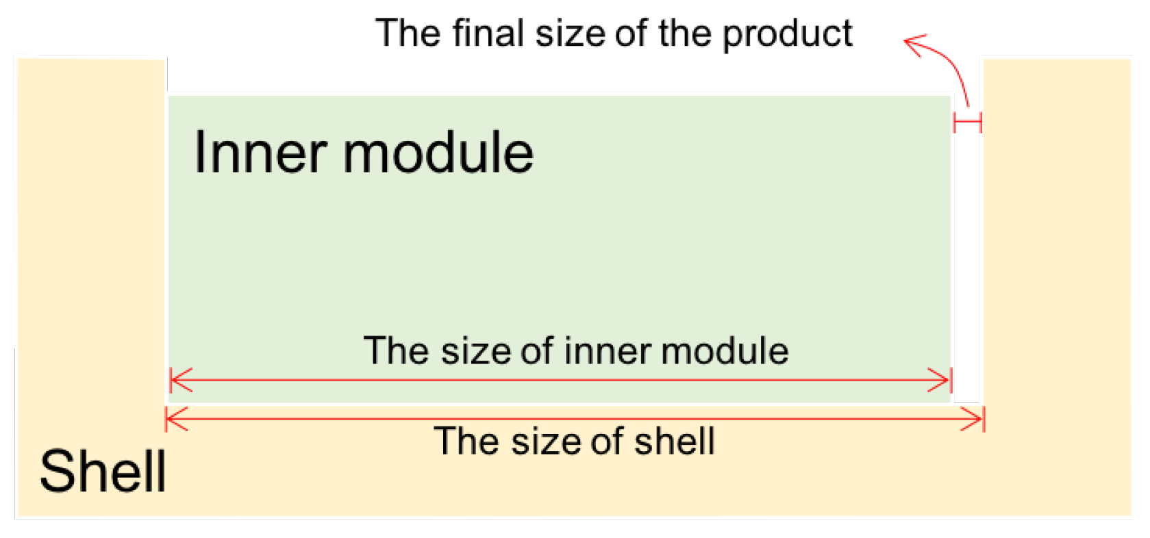
Figure 1 is the sectional drawing of a product that consists of two parts: shell and inner module. The assembler receives three workpieces per part, and the size of each workpiece is listed in
Table 1. The inner module is installed in the shell, so the assembler should take one inner module and one shell and then installs them together. There is a gap between the inner module and the shell as shown in
Figure 1, and we call the gap as the final size. Supposing the final size of the feasible product is bounded by 0 and
, we can use the final size to evaluate the feasibility of the given assembly guidance (AG). For example, after receiving the assembly guidance
, the assembler installs the shell number 1 and the inner module number 1, the shell number 2 and the inner module number 2, and the shell number 3 and the inner module number 3 together. The final sizes are
,
, and
, respectively, and
is feasible. However,
is infeasible. The final sizes are
,
, and
in
, and the final sizes of the first and third products are not acceptable, so
is infeasible.
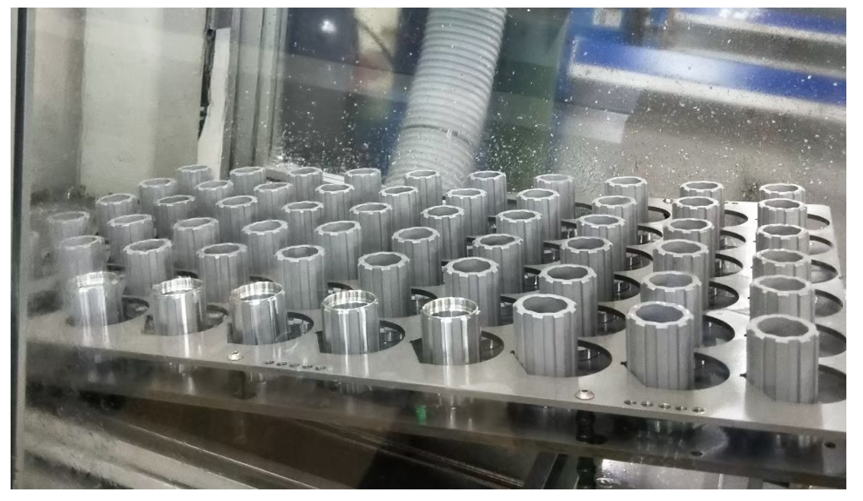
In the assembly line, the assembler receives some workpieces as shown in
Figure 2 and the installation specification including the assembly instructions and the assembly process. The assembler randomly or sequentially picks up a workpiece of each part and then installs the workpiece one by one. Once the unacceptable final size is detected, the assembler will consider the secondary processing to fix the final size. However, the secondary processing is inappropriate, because the secondary processing only fixes a portion of size and lack for the dimensional chain evaluation [
5,
6]. So, the module’s quality can not be guaranteed.
An appropriate solution is to compute the AG in advanced, and the AG guides the assembler to install the products. Therefore, the properties of the products are controlled by the AG. To compute the AG, we have some considerations:
The sustainability: most production lines in the industry 4.0 factories provide non-stop works except for the maintenance. So, the AG computation must cover all kinds of product assembly processes that includes different number of workpieces and parts, the assembly sequence, the final size, etc.
The minimization of computation time: the AG computation can not disturb the assembly process. Once the assembly process is postponed because of the delay of the AG computation, the utilization of the assembly line is decreased. The AG computation can be processed while the workpieces are moving, and the AG can be prepared when the assemblers receive all workpieces.
The guarantee of product quality: when the assembler follows the assembly instruction provided by the AG, all output products are acceptable. In other words, the AG computation has to guarantee the product quality.
To reach the necessary listed above, we first formulate the AG computation as the dimensional chain assembly (DCA) problem, and the goal of DCA problem is to output the acceptable AG for assemblers. We prove that the DCA problem is a NP-complete problem, and the search algorithms [
7,
8] requires huge computation time to find the optimal solution. The requirement of the minimum computation time is violated. The combinatorial optimization techniques help us to compute the optimal solutions [
9], but the combinatorial optimization algorithms may be modified for installing new products. So, we survey the general optimization approaches that are satisfied with the sustainability. We adopt the single-solution evolution (SSE) to reach the consideration of the minimum computation time. To guarantee of product quality, we modify the simulated annealing (SA) algorithm to design the assembly guidance optimizer (AGO) to calculate the AG.
To evaluate the performance of the proposed AGO, we build a Windows-based platform to simulate the AG computation, and measure the performance of the AGO. We obtain following properties from the simulated results:
The sustainability: the assemblers obtain the AG from the proposed AGO in the different DCA problems (to install various products). So, the assembly manager can use the AGO to compute the AG sustainably.
The minimization of computation time: the AGO outputs the AG for installing thousands of workpieces in few seconds, and the computation is finish before all workpieces arrive at the assembly line.
The guarantee of product quality: the final size of all products are satisfied with the product specification, and the AG outputted by the AGO provides high solution quality.
Moreover, given an assembly configuration of the AGO, the increase of the computation time and the decrease of the solution quality is linear to the problem scale. It means that the computation time and the product quality of the AGO can be predicted by the scale of the assembly instance. Therefore, the AGO can be applied to the real-world assembly lines for computing the AGs of various products.
2. Related Works
Calculating the optimal solution with minimum gap between the product size and the ideal size in the DCA problem can be reduced to the exact weight perfect matching problem from a given bipartite graph. Therefore, solving the DCA problem is NP hard, as shown in
Section 3.3. There are two major approaches of solving the DCA problem, and they are listed as follows:
Greedy algorithms: deriving the near-optimal or optimal (when the instances meet the specific condition) solutions by the problem properties [
10,
11].
Soft-computing algorithms: deriving the near-optimal solutions by continuously refining the solution quality [
9,
12,
13,
14,
15].
Greedy algorithms output the solutions efficiently, but the optimal solution is not guaranteed. Soft-computing algorithms seek the solutions with better quality one by one, so soft-computing algorithms require more computation time than that of greedy algorithms. Moreover, because greedy algorithms are problem-based approaches, the algorithms should be modified in solving different problems. Therefore, the soft-computing algorithms are more appropriate than greedy algorithms in terms of the industrial purpose.
Although the soft-computing algorithms require more computation time to derive near-optimal solutions, we still can get the acceptable solutions in a short period of time because of the increase of the computation power. Therefore, soft-computing algorithms are applied to broad-range applications, such as the decision evaluation in the banks [
14,
16], the timetable calculation of the train scheduler [
17,
18], the vehicle route determination [
19,
20], etc.
Soft-computing algorithms are classified into two categories: the single-solution evolution (SSE) [
12] and the multiple-solution evolution (MSE) approaches, e.g., such as genetic algorithm [
14,
21], particle swarm optimization [
22], and ant colony optimization [
23]. In each iteration, the SSE approaches only consider one solution while some solutions are evaluated by the MSE approaches. The SSE approaches output the improved solutions rapidly [
12,
13], and the solution quality is continuously improved. On the other hand, MSE approaches require more computation time to finish an iteration, but MSE approaches have higher probability in obtaining better solutions than SSE. Therefore, SSE approaches are more appropriate than MSE approaches based on the industrial consideration, and we apply the SSE approach to design the AGO.
The local search approaches [
24] and the simulated annealing (SA) [
12,
13] are popular SSE approaches. The local search approaches consider problem properties to search the solutions with higher quality. SA applies the annealing idea to approximate optimal solution iteratively for the discrete solution space. SA covers broader range applications than local search approaches. Therefore, SA is more appropriate than local search approaches because the assemblers have to install various products in the assembly lines.
4. Proposed Solution
According to the survey of feasible approaches listed in
Section 2, we apply the SA algorithm to design the AGO for computing the assembly guidance with
. The algorithm of AGO is shown in Algorithm 1. The AGO receives a DCA instance
D, an initial temperature
T, a temperature descent rate
r, and a maximum number of iterations
. The AGO outputs an assembly guidance
. Firstly, the AGO generates an initial solution
in line 1. Then, the AGO enters a solution refinement loop for seeking better solutions from lines 2 to 8. When meeting the stop conditions, the AGO exits the loop and return the refined solution
. In the refinement loop, the AGO picks up a neighbor solution
based on
and then evaluates the acceptance of
by the quality of
and the current temperature. In the last step of the solution refinement loop, the temperature is reduced by
r. Here, we show the details about the AGO algorithms.
| Algorithm 1: The algorithm of the proposed assembly guidance optimizer (AGO) for DCA. |
![Sustainability 12 04690 i001]() |
The solution encoding: the solution structure is defined as
in
Section 3.1. However,
is sparse because only
m elements are meaningful for each product. Therefore, we design another data structure for reducing the memory usage and increasing the computation efficiency for the implementation consideration. Two solutions listed in
Table 2 are transformed to the format as shown in
Table 3. The column indicates the part information while each row represents the selected workpieces in a product. Each element in the solution is the workpiece index. So,
provides higher readability for the assembler. In the solution 2, for example, the first product considers workpiece 1 of part A and workpiece 3 of part B, the second product considers workpiece 2 of part A and workpiece 1 of part B, etc. Moreover, the format of
is still satisfied with the constraints listed in
Section 3.1.
The initial solution generation: the AGO apply the random process to construct the initial solution. The AGO is designed for installing various products. Because the assembly processes and the properties of various products are different, considering the random initial solution increases the coverage of the search directions. For an initial solution , each workpiece is picked up randomly without putting back and inserted into an arbitrary product.
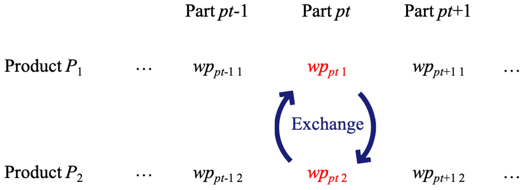
The neighbor solution generation: we refer to the “royal road” function [
26] to design a neighborhood search approach. The algorithm named by
is illustrated in Algorithm 2.
receives two parameters: the base solution
and the variation degree
v.
outputs a solution
based on
, and
v determines the difference between
and
. Firstly,
copies
to
. Then,
picks up one part and two products as shown in lines 3 to 5. Then, the workpieces of the selected products are swapped as illustrated in
Figure 3. Iteratively executing the exchange process for
v times. Therefore,
v controls the variation degree of
and
.
The stop condition: the AGO considers the maximum iteration and the minimum temperature as the stop condition. The value of given by the assembler manager controls the running time of the AGO. According to the annealing concept, the temperature is continuously reduced to the room temperature, so the room temperature is also another stop condition. By considering the linear temperature reducing function, we assume the room temperature is 0 C. Therefore, the temperature could be very closed to zero but not smaller than zero. The maximum number of iterations or the minimum temperature will not dominate the stop condition, and the temperature reducing function can work together with the maximum number of iterations.
The acceptance criterions of the neighbor solutions: the AGO computes the
by the difference between the solution quality between
and
, i.e.,
. For
, i.e.,
, the quality of
is better than that of
, and the AGO accepts
. On the other hand, the AGO simulates the Boltzmann distribution [
27] to determine the probability of accepting
. According to the property of the Boltzmann distribution,
with lower quality is accepted easily in the early stage. The AGO is designed to discover as wide as possible, so the probability of accepting the solution with worse quality in the early stage is higher than that in the late stage. The neighbor solution acceptance concept is listed in lines 4 to 7 in Algorithm 1.
| Algorithm 2: () The algorithm of the neighbor solution generation. |
![Sustainability 12 04690 i002]() |
5. Simulation
The AGO provides high flexibility for the assembly processes of various products. The assembly manager has to determine the AGO configurations to compute the assembly guidance. Therefore, we first compute the optimal configuration before evaluating the performance of the AGO. Next, we apply the derived configuration to evaluate the AGO performance including the computation efficiency and the solution quality.
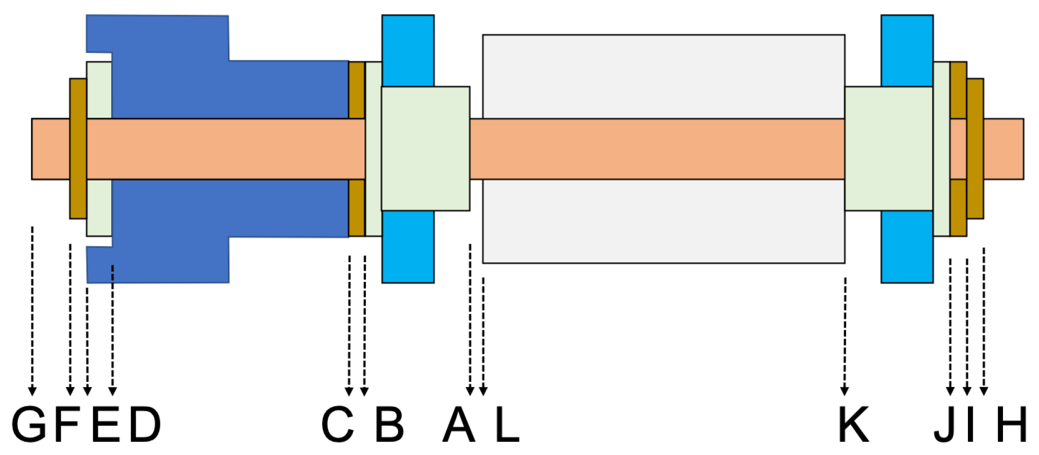
We consider the countershaft module as shown in
Figure 4 to be the simulated target [
28]. In this case, each product consists of 11 parts, i.e.,
. The letter from A to L in
Figure 4 represents a cutting plane, e.g., AB, BC, CD, DE, EF, FG, GH, HI, IJ, JK, and KL. All workpieces are installed in the central columella, so all cutting planes are in the same dimensional chain. Therefore, we have
for the sequence of AB, BC, CD, DE, EF, FG, GH, HI, IJ, JK, and KL. We consider
,
, and
. Given
n workpieces for each part, the assemblers receive
workpieces in total, and output
n countershaft modules.
We consider the personal computer as the simulation platform with Windows 10. The platform equips Intel i7 CPU, 16 GB memory, and 512 GB SSD while the AGO is implemented by C# in Visual Studio 2015.
5.1. Configuration Evaluation
We consider 1500 workpieces for each part, e.g.,
. The AGO configuration includes
T,
r,
, and
v. We focus on evaluating the settings of
T,
r, and
, and
is applied to the configuration evaluation. The considered configurations are:
T from 5000 to 50,000 with gap 5000,
r from 0.9 to 0.99 with gap 0.01, and
from 1000 to 5000 with gap 1000. For each configuration, we run 10 times and use the average values to be the evaluation results. We consider the average CPU time and the average solution quality as defined in Equation (
2) to measure the configuration quality.
5.1.1. Solution Quality Evaluation
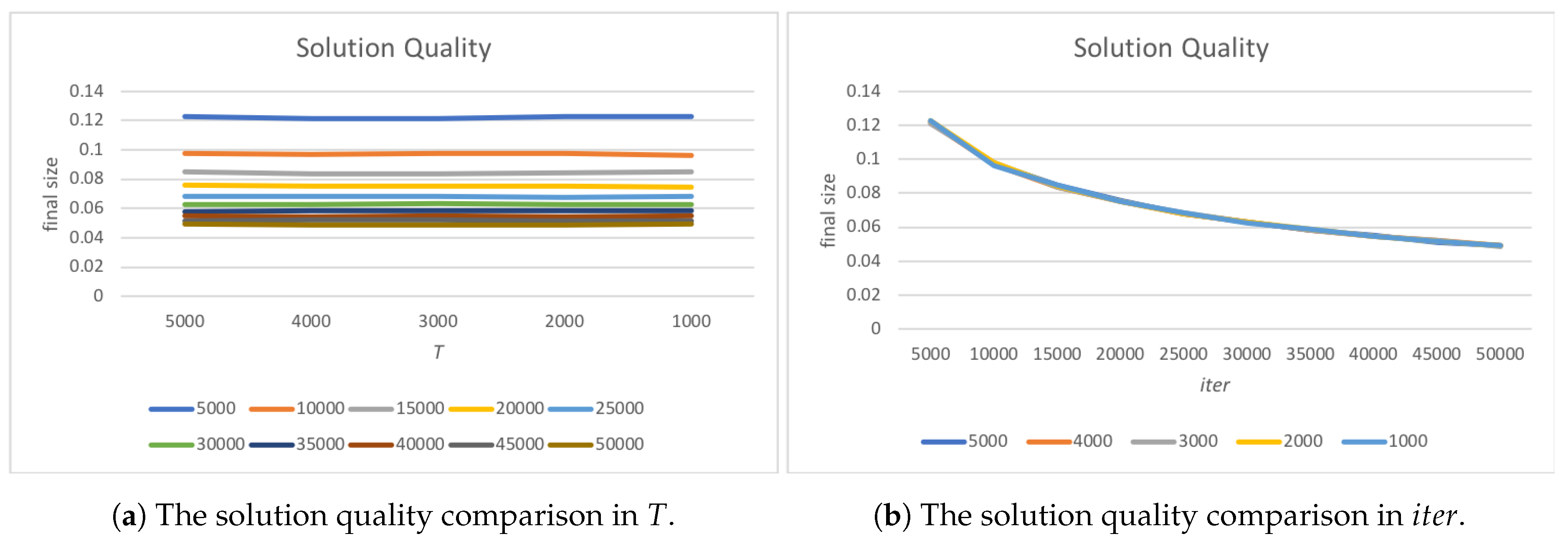
The final size of each product is the major concern for the assembly manager. We first investigate the solution quality for all parameter combinations to find out the appropriate configurations that will be applied to the next-step simulations.
Figure 5 lists the solution quality results defined in Equation (
2) for all combinations with
and
T under
. We have following observations:
The distribution of the solution is similar for various settings of
r. The results in
Figure 5 is captured in the configurations with
, and the distribution is similar to that captured in other settings of
r. So, we just illustrated the results with
.
The difference of the solution quality between various settings of
T is small from
Figure 5b, and the solution quality is not improved dramatically by increasing the initial temperature.
Higher settings of
lead to better solution quality in
Figure 5a because the solutions can be refined for longer search time.
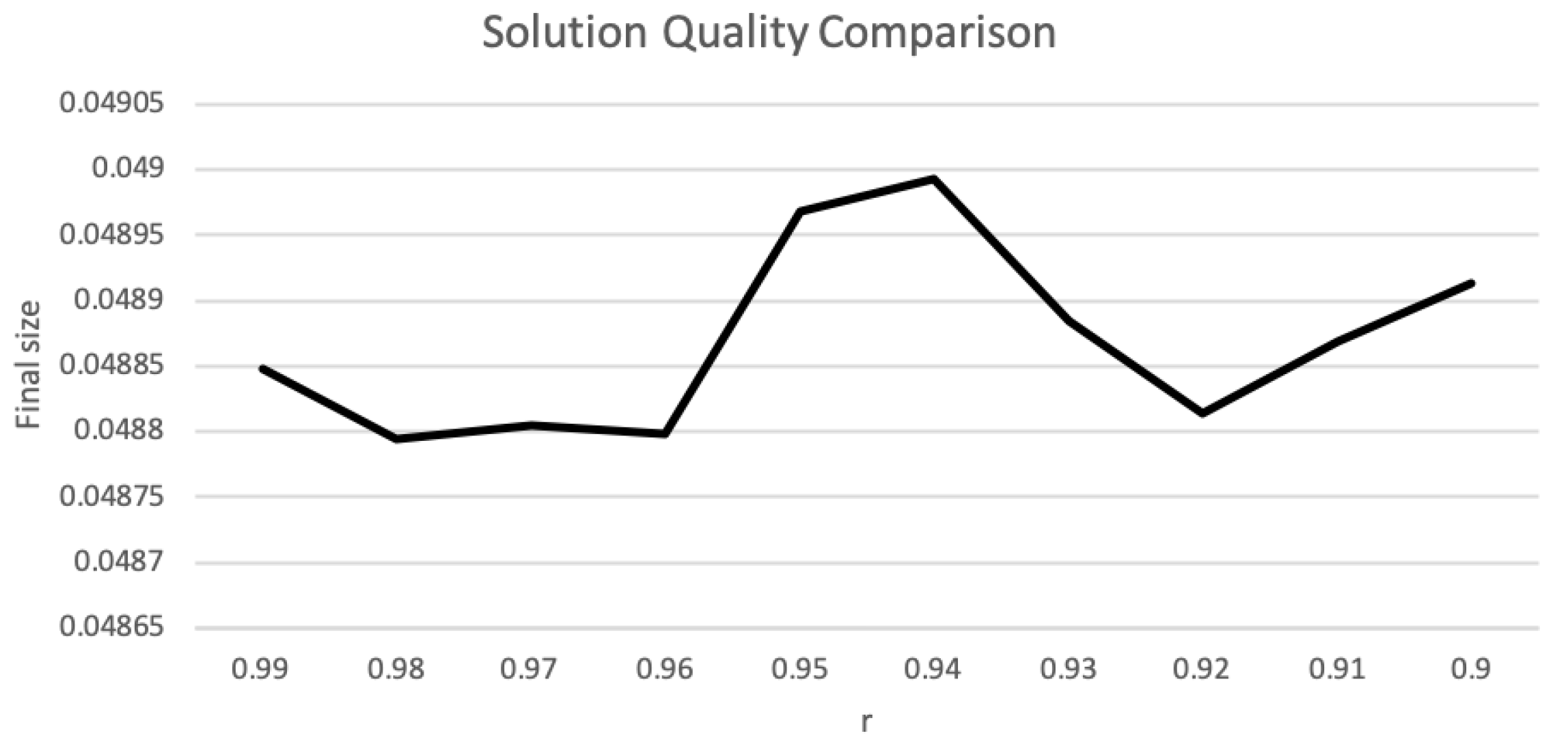
From the above observations, the settings of
T and
are not the critical parameter, so we evaluate the setting of
r. We capture the best solution from all settings of
r, and the results are listed in
Figure 6 and
Table 4. The result shows that the setting
provides minimum final size. Therefore, we will consider
in the following simulations.
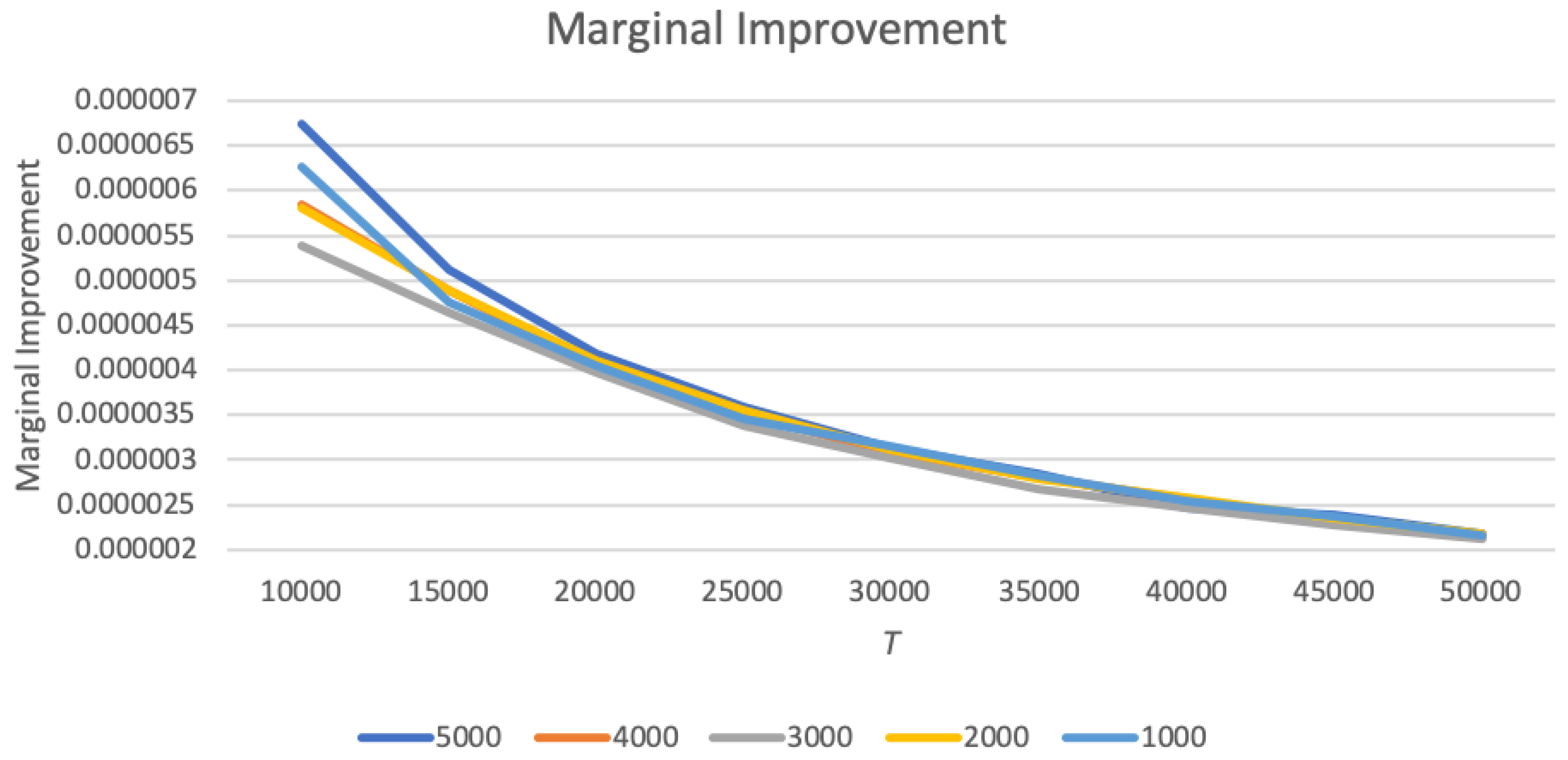
5.1.2. Marginal Improvement Evaluation
From the results listed in
Figure 5, the solution quality is improved by increasing the number of iterations. Therefore, we compare the marginal improvement for the settings of
and
T. The marginal improvement is defined as:
Given the settings of
and
T with
,
stands for the difference of the final gap between
and
while
represents the gap of the running time. Equation (
5) shows the improvement ratio of the solution quality to the running time. Therefore, maximizing the values of
is the objective in this simulation.
We have the results illustrated in
Figure 7. The
curves are descending for all configurations as increasing the settings of
. However, the maximum
takes place from the configurations with
and
. The result is reasonable, so we will use this configuration to evaluate the performance of the proposed AGO.
5.2. Performance Evaluation
We consider
,
, and
in the following experiments for measuring the AGO performance. We generate 10 instances for
, and 2000. We run the AGO 10 times for each instance and use the averaged value for each configuration. The results in terms of the running time and the solution quality are illustrated in
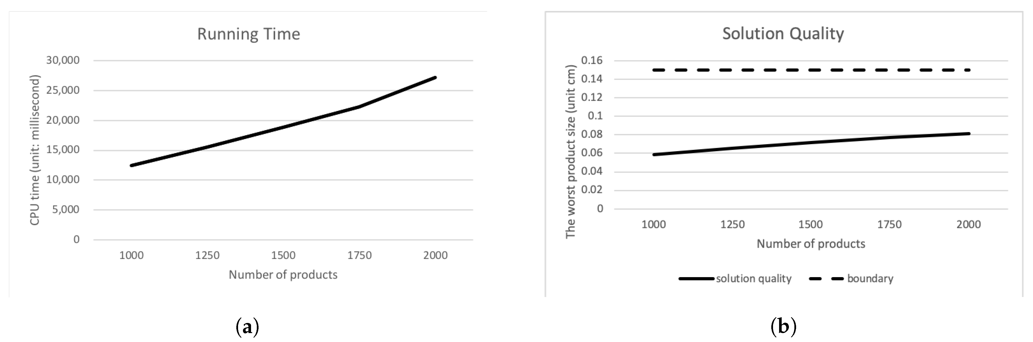
Figure 8.
The curve of running time is linearly raised by the number of products. The AGO requires more computation time in each iteration of larger scale instances. So, this is the major reason for the raised computation time even if the AGO parameters are the same. The AGO uses 25 seconds approximately to compute the assembly guidance in the instances with workpieces. The running time is acceptable for the implementation consideration.
The gap between the product size and the ideal size is getting bigger for large scale instances. The AGO requires more computation time to maintain the same solution quality in the large-scale instances. The size of the search space is increased exponentially by the instance scale, e.g., the number of workpieces, so the solution quality is decreased by the number of the products in the same AGO configuration. The averaged gap between final size and is slightly increased from 0.0589 to 0.0816 without providing more computation resource.
The running time is increased and the solution quality is decreased by scaling up the problem size, but the variance amount is linear. It means that the assembly manager can estimate the running time and the solution quality from the problem scale, and the configuration is unnecessary to be re-evaluated. The configuration of AGO should be re-evaluated only when the solution quality is very close to the target or over , where the products are near unacceptable.
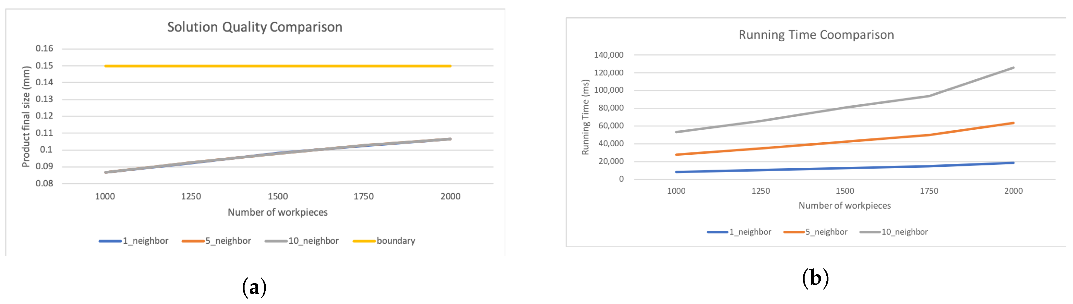
5.3. Search Breadth Evaluation
Single solution refinement is the major property of the SA, and the neighbor solutions can be carefully evaluated rather than the wide search. However, the solution quality is difficult to be improved dramatically in the SA. We are interested in the effect of the search breadth, so we estimate the performance of the AGO with different degrees of the search breadth. There are two ways to increase the search breadth: increasing the number of the population size, and increasing the degree of the local search. Since the SA is an SSE approach, we do not increase the number of the population size. Thus, we evaluate some neighbors in the local search approach to increase search breadth. We consider 1, 5, and 10 neighbors in each experiment and evaluate the running time, the solution quality, and the computation efficiency for the configuration with
,
, and
. The solution results are illustrated in
Figure 9.
From the results in
Figure 9a, the solution quality is not improved by increasing the number of evaluated neighbors. On the other hand, it is rational to receive that the running time is increased in high number of neighbors as shown in
Figure 9b. Increasing the search breadth is profitless in improving the solution quality. Therefore, the AGO with the single neighbor evaluation process is efficient and outputs high-quality solution.
6. Conclusions
In this paper, we define the DCA problem and prove the problem is NP-complete by the reduction from the exact weight perfect matching problem. We propose a SA-based approach that is named as AGO to resolve the DCA problem. The AGO considers 5V properties of the assembly process. The simulation results show that the problem scale leads to the linear effect on the solution quality and the running time. Therefore, the assembly manager can easily estimate the running time and the solution quality. Moreover, the AGO provides appropriate search strategy, and it is unnecessary to search multiple solutions simultaneously. So, the near optimal solution can be calculated efficiently.
There are some variance models of the DCA problem. For example, a target product may have several dimensional chains. The dimensional chains may cross on a special part, so the AGO has to make sure that the requirements of all dimensional chains can be satisfied in a target product. Based on the current progress, we have begun modeling the multi-dimensional chain problem, and we will apply the AGO to resolve the multi-dimensional chain problem where that is close to the real-world assembly goal.

 ,
, 


