Influence of Land Use/Land Cover on Surface-Water Quality of Santa Lucía River, Uruguay

Abstract

Land use/land cover is one of the critical factors that affects surface-water quality at catchment scale. Effective mitigation strategies require an in-depth understanding of the leading causes of water pollution to improve community well-being and ecosystem health. The main aim of this study is to assess the relationship between land use/land cover and biophysical and chemical water-quality parameters in the Santa Lucía catchment (Uruguay, South America). The Santa Lucía river is the primary potable source of the country and, in the last few years, has had eutrophication issues. Several multivariate statistical analyses were adopted to accomplish the specific objectives of this study. The principal component analysis (PCA), coupled with k-means cluster analysis (CA), helped to identify a seasonal variation (fall/winter and spring/summer) of the water quality. The hierarchical cluster analysis (HCA) allowed one to classify the water-quality monitoring stations in three groups in the fall/winter season. The factor analysis (FA) with a rotation of the axis (varimax) was adopted to identify the most significant water-quality variables of the system (turbidity and flow). Finally, another PCA was run to link water-quality variables to the dominant land uses of the watershed. Strong correlations between TP and agriculture-land use, TP and livestock farming, NT and urban areas arose. It was found that these multivariate exploratory tools can provide a proper overview of the water-quality behavior in space and time and the correlations between water-quality variables and land use.

1. Introduction

Water quality plays a vital role in ecosystems protection, public health, agriculture, and industry [1]. The water pollution sources not only come from rivers and lakes, but also from the land use/land cover (LU/LC) and human activities [2]. LU/LC is the carrier of anthropogenic activity in catchments. Landscape patterns control several biochemical and physical processes within the watershed. Thus, one of the significant consequences of landscape pattern change is the worsening of stream-water quality [3]. Water pollution not only leads to the inequity of river ecosystems, but also threatens socio-economic sustainability and public-health safety [4]. With the aim of adopting effective actions for the protection of surface-water bodies, a scientific interpretation of the relationship between LU/LC and river-water quality is critically needed. However, the interactions between LU/LC and water quality are challenging to evaluate, because of the complexity of the processes and the massive number of variables and parameters involved [5,6].

Many studies have investigated the relationship between water quality and land use. Some of them have been performed in small watersheds with a high sampling frequency at a few monitoring stations [7], or in larger basins with a low sampling frequency (monthly or seasonally), but at several monitoring sites [8,9]. For example, many investigations have demonstrated that settlement areas and farmland are responsible for water degradation, while forested regions have negative correlations with most ions [10,11]. Kersebaum et al. estimated that the contribution of agricultural activities as diffuse source pollution of surface waters is about equal to 55% in European countries [12]. These relationships have often been explored concerning strategies for improving water quality at a smaller catchment scale. Continuous advance of GIS-based tools and more refined data sources support approaches at larger scales. However, little is known on the relationship between LU/LC and the water quality affected by multiple point and diffuse sources of pollution in heterogeneous watersheds. These tasks have been recently tackled by different conventional multivariate techniques [13]. For instance, Kändler et al., in a transboundary basin located in Germany and the Czech Republic, proved with the aid of a cluster analysis that arable land rules water quality when its proportion of the subcatchment area is >40%; while a forest proportion higher than 70% leads to water quality with a low concentration of nutrients and heavy metals [6]. Dutta et al. adopted principal component analysis (PCA) along with cluster analysis to identify municipal wastewater discharge as the main factor of the deterioration of the water quality of the Nag River (India) [14]. Namugize et al. used the Pearson correlation coefficient to demonstrate the strong relationship between the increasing nutrient concentration in the Umgeni river (South Africa) and the expansion of urban/built-up areas and cultivation lands [15]. Therefore, further research is needed to integrate LU/LC effects on water quality over several years, considering a variety of compounds originating from non-point sources of pollution.

Based on these considerations, with this work, we aim to enrich this body of knowledge with an application of several multivariate techniques in the Santa Lucía watershed, located in Uruguay (South America). Santa Lucía is one of the main fluvial systems of the country for its ecological characteristics, location, and functions. Its watershed delivers water for about 60% of the Uruguayan population (1.6 million people) and supports several agro-industrial activities, being a major region of food production for the country [16]. Anthropic activities led to water quality deterioration of the fluvial system, which has experienced a progressive eutrophication process. In March 2013, a cyanobacterial bloom (Dolichospermum sp.) with high geosmin production caused taste and odor in drinking water, affecting drinking water supply for most of the country’s population. This generated public alarm and caused government concern, which consequently promoted the “Action Plan for the Protection of Environmental Quality and Availability of Drinking Water Sources in the Santa Lucía River Basin,” and the creation of the Santa Lucía River Basin Commission [17,18].

Consequently, the purpose of this study is to provide answers to the following scientific questions: (i) which are the primary water-quality variables that alone can characterize the Santa Lucía system? Furthermore, (ii) which compounds are significant indicators for particular land-use categories?

The specific objective is threefold: (i) analyze temporal and spatial patterns of biophysical and chemical water-quality variables based on the free-access national dataset; (ii) identify relationships between LU/LC categories and water-quality variables; (iii) evaluate the efficiency of the adopted multivariate statistical techniques in interpreting surface-water quality and pollutant interactions in this part of the world.

Accordingly, the results of this study are expected to enhance the understanding of the relationships between land use and surface-water quality around the world, and, thereby, facilitate informed decision making in the design of measures to mitigate pollution impacts on receiving waters’ bodies.

2. Materials and Methods

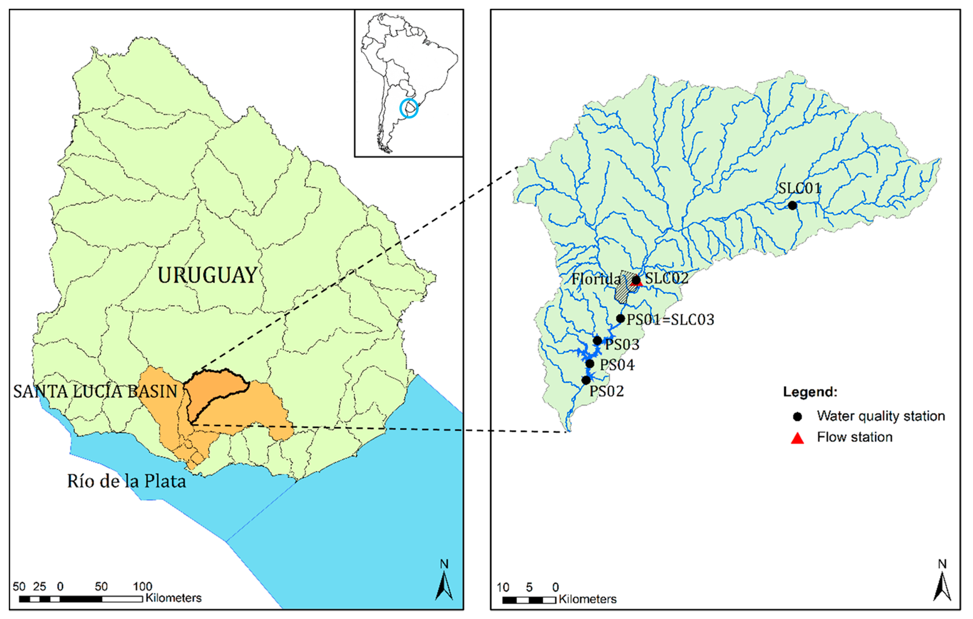
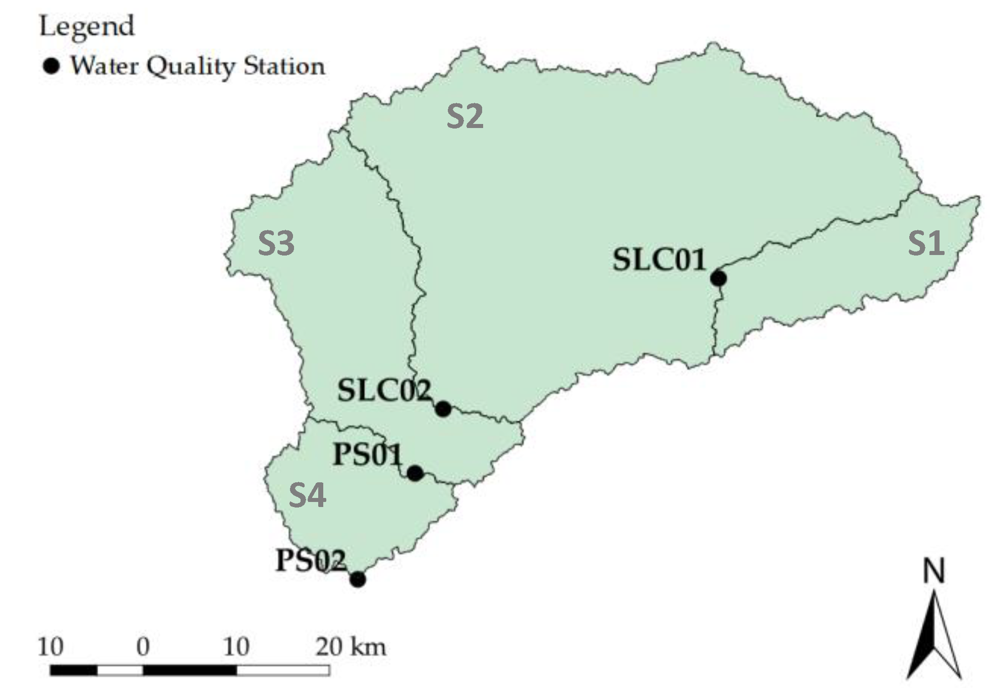
2.1. Study Area

The Santa Lucía (SL) watershed (highlighted in orange on the left side of Figure 1) is located in a temperate climate zone in south Uruguay, between 33°42′ S–34°50′ S and 55°00′ W–57°06′ W. This catchment is the primary source of drinking water in the country, as it allocates water for 60% of the Uruguayan population, and also supports several agro-industrial activities [16,19]. The SL watershed has a primary drinking water reservoir, Paso Severino (PS), operative since 1987, located in Santa Lucía Chico (SLC) basin, a subcatchment of SL (right side of Figure 1). PS has a storage capacity of 65 hm³, a surface area of 15 km² and a maximum depth of 20 m. Its drainage area is 2500 km². The purifying plant of Aguas Corrientes is located 50 km-downstream of the reservoir.

Taking into account the strategic importance of SL watershed for the country, it is fundamental to have adequate water-resource management policies to guarantee a sufficient water-quality threshold, to satisfy all water uses and avoid environmental conflicts. Based on these considerations, SLC was selected as a case study.

The SLC basin is entirely located in the Florida department, and its surface is equal to 2570 km². Its elevation ranges between 200 m a.s.l. in the north-eastern part of the basin, and 25 m a.s.l. at the PS reservoir. The catchment stands on granitic gneiss rocks of the Piedra Alta Terrane. The Brunosolic soil is dominant in this area with loam texture and rich in soil organic matter, with higher clay and silt proportions in the southern part. The climate is temperate, with four different seasons. It is characterized by total annual precipitation that varies between 1000 mm and 1500 mm and a temperature that can vary between 3 °C and 30 °C [20].

2.2. Data Collection

The streamflow data set considered in this work corresponds to the period 2004–2018 and is measured by the Uruguay National Water Board (DINAGUA). The streamflow is obtained three times a day from the water level measured at the hydrometric station located in Florida city (Figure 1).

The water-quality dataset used in this study belongs to the Uruguayan National Environment Board (DINAMA) and is freely downloadable from the National Environmental Observatory (OAN) [21]. The data were collected bi-monthly, from 2004 to 2018, at six monitoring stations located along the Santa Lucía Chico river (Figure 1). It is worth noting that three of these stations (PS03, PS04, and PS02) are located in the PS reservoir, while SLC01, SLC02, and PS01 are located upstream of the reservoir.

The DINAMA—Department of Monitoring of Environmental Components carried out the water-quality monitoring campaign, within the framework of the Global Environment Monitoring System for Water (GEMS/Water) of the United Nations. Among the variables considered, DO was measured in situ, while the other variables were defined in the DINAMA Environmental Laboratory following the procedures of the “Analytical procedures guide for environmental samples” [22].

The following variables were considered for this study: total phosphorus (TP), total nitrogen (TN), nitrate (NO₃⁻), nitrite (NO₂⁻), ammonium (NH₄⁺), turbidity, water temperature (T), dissolved oxygen (DO), biochemical oxygen demand (BOD₅), and flow rate (Q).

It is worth remarking that the water-quality variables considered in this work are related to the eutrophication problem that characterizes the water bodies of the study area and the LU/LC changes.

The current national LU/LC map (2018) with a scale of 1:50,000 was obtained from the Ministry of Livestock, Agriculture, and Fisheries (MGAP) [23].

2.3. Trophic State Index (TSI)

The trophic condition of the SL river was assessed using TSI values and calculated as follows [24,25]:

$$TS{I}_{stream}=10·\left[6-\frac{0.42-0.36·\ln \left(TP\right)}{\ln \left(2\right)}\right]-20$$

(1)

where TP is the measured total phosphorus concentration [μg/L].

The TSI_stream ranges from 0 to 100, with high values representing high eutrophication levels. The trophic status for streams is classified into six grades based on the TSI scores: ultra-oligotrophic (TS_Istream ≤ 47), oligotrophic (47 < TSI_stream ≤ 52), mesotrophic (52 < TSI_stream ≤ 59), eutrophic (59 < TSI_stream ≤ 63), super-eutrophic (63 < TSI_stream ≤ 67) and hyper-eutrophic (TSI_stream > 67). The eutrophication status of the three sampling sites located in the mainstream (SLC01, SLC02, and PS01) was calculated by using Equation (1).

For evaluating the trophic condition at the monitoring stations located in Paso Severino reservoir (PS02, PS03, and PS04), a modified Carlson Index proposed by Lamparelli was used [26,27]. It is also based on total phosphorus (TP) concentration and is calculated with the following equation:

$$TS{I}_{lake}=10·\left[6-\frac{1.77-0.42·\ln \left(TP\right)}{\ln \left(2\right)}\right]$$

(2)

where TP is the measured total phosphorus concentration [μg/L].

As well as TSI_stream, TSI_lake is classified into the same six grades previously described.

2.4. Data Analysis

2.4.1. Multivariate Statistical Analysis

Conventional multivariate data-analysis techniques, cluster analysis (CA) (hierarchical cluster analysis (HCA) and k-means) and principal components analysis/factor analysis (PCA/FA), were used in this work. Both algorithms were coded and run in R, using the libraries “cluster,” “HSAUR,” “vegan,” “devtools,” and “ggbiplot” [28]. Being these unsupervised techniques methods, they were used as exploratory data analyses, where the aim is hypothesis generation rather than hypothesis verification.

To assess temporal and spatial trends of biophysical and chemical water-quality variables, HCA and k-means were used in this study. CA groups the objects (data points) into classes (clusters) based on their similarities within a class and dissimilarities among different clusters [29]. Initially, the similarity is computed among data points. Afterwards, once the data points start to group, the similarity is calculated among the clusters as well [30,31]. The clustering algorithm is also sensitive to the similarity (or distance) measures [32].

PCA was used to identify relationships between LU/LC categories and water-quality variables. PCA reduces the dimensionality and complexity of a dataset of independent variables. It is a technique that creates a new variable-set containing orthogonal-uncorrelated variables, which are linear combinations of the original attributes and are ordered by decreasing variance. These new variables are known as principal components (PCs) [33]. They have the advantage of gathering possible emerging properties of the system that, instead, could be hidden if we focus only on the physical meaning of each original variable [34]. For this reason, PCA was chosen for this study. The eigenvalues measure the significance of the PCs. Factor loadings quantify the correlation among PCs and original variables. Scores represent the individual transformed observations [35]. Afterwards, factor analysis (FA) was adopted, since it reduces the contribution of less important attributes obtained from PCA, and the new group of variables, called varifactors (VF), is obtained through a rotation of the axes defined by PCA. While a PC is a linear combination of measured water-quality variables, a VF can include latent variables [36]. The varimax rotation, the PCs rotation adopted in this study, maximizes the sum of the variance of the squared loadings. This usually results in high factor loadings for a smaller number of variables and low factor loadings for the rest.

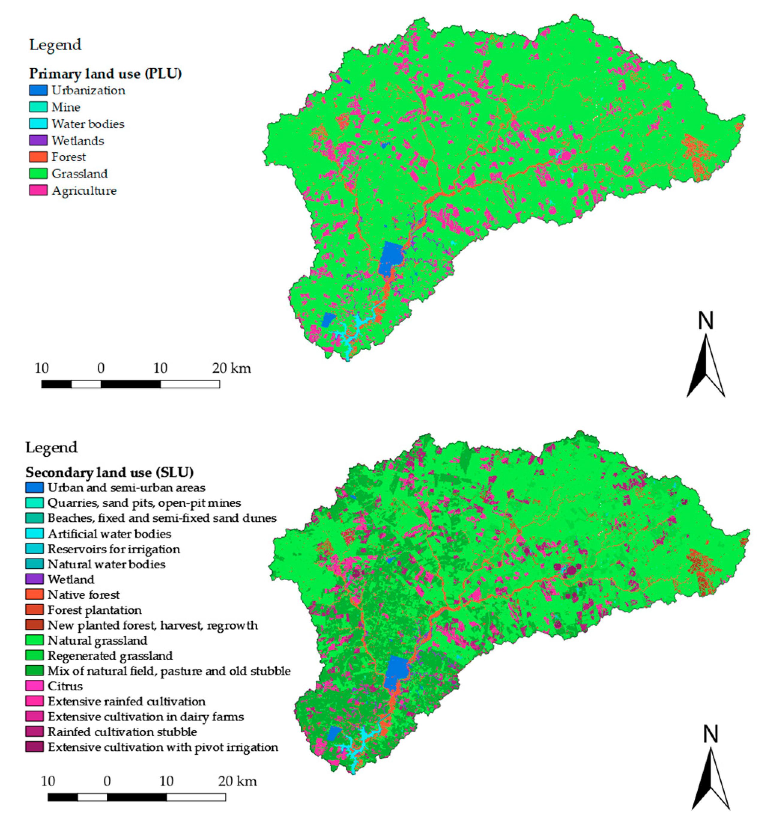
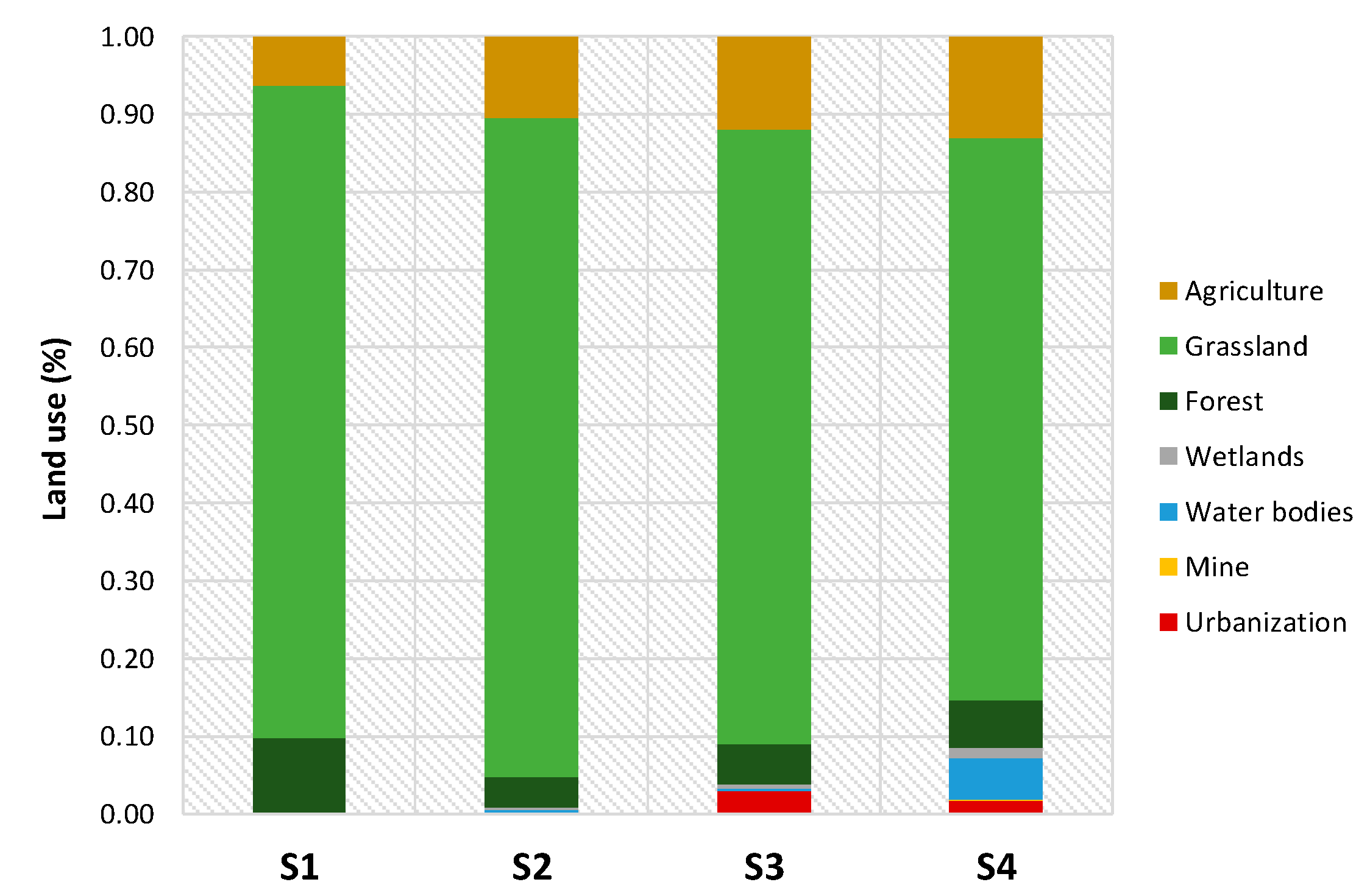
2.4.2. Land Use/Land Cover Reclassification

Using QGIS 3.10, a reclassification of land use and land cover in the SLC watershed was carried out, with the aim of merging similar categories into a single class. Primary land use (PLU) and secondary land use (SLU) were defined as the reclassification map and the original detailed map, respectively. The PLU categories identified were agriculture (AGR), grassland (GRAS), forest (FOR), wetlands (WET), water bodies (WATB), mine (MIN), and urbanization (URB) (Figure 2). In the Supplementary Materials, a comprehensive table that shows the land-use reclassification is reported (SM-1).

A catchment delineation exercise was carried out upstream of each sampling point, to quantify the proportion of land-use categories that contributed to a sampling site. Automated hydrologic tools of QGIS 3.10, for a digital elevation model (DEM) of 30m × 30m resolution, were used. Based on four sampling points (SLC01, SLC02, PS01, and PS02), the catchment was divided into four sub-catchments (

Table 1. Subcatchment delineation based on water-quality monitoring stations.

Subcatchment ID	Area (km2)	Water-Quality Monitoring Station	Latitude	Longitude
S1	244	SLC01	−33.96	−55.88
S2	1504	SLC02	−34.09	−56.20
S3	510	PS01	−34.15	−56.24
S4	216	PS02	−34.26	−56.30

, Figure 3). It is worth remarking that the monitoring stations located inside the reservoir were not taken into account (PS03 and PS04).

Percentages of the LU/LC classes were then calculated for each subcatchment. In Figure 4, the land use percentages of the non-incremental subbasins are represented, with the aim of showing the spatial distribution of the SLC LU/LC. All over the watershed, the dominant land use is grassland. From upstream to downstream, agriculture class increases, while grassland-land use decreases. Furthermore, it is interesting to see that, in the upstream portion of SLC watershed, in the last years, there has been a significant percentage of forest plantation, due to wood production for the paper industry. At S3, a not-negligible part of the subcatchment is occupied by urban areas (the principal city of the entire region, Florida city, is located here). At S4, a significant percentage of native forest and water bodies can be found, due to the presence of the PS reservoir.

In particular, the north-eastern part of the catchment is characterized by superficial soils, with rocky areas, natural fertility, and no high drought risk. For this reason, extensive sheep farming and forest plantation mainly occur in this region. In the central portion of the basin, soils with high natural fertility, slow permeability, and medium drought risk are more frequent. This type of soil allows the agricultural production of cereal and oilseed crops, cattle farming, and intensive dairy activity associated with forage production. In the southern area, the soils have high fertility, high depth, and medium drought risk. Horticultural and farm production organized on family farms are presented here [37].

2.4.3. Extraction of Land-Use Related Parameter: Shannon’s Diversity Index

As noted, land use can negatively impact the pollutant loads entering water bodies, since it is strongly associated with anthropogenic activities [38]. Recent investigation findings have shown that LU/LC class alone is inadequate to characterize pollutant inputs to the natural environment, such as surface water [39,40]. This is due to the fact that, even within the same land-use category, configurations such as land-development layout might be significantly different. For instance, at our study basin that is livestock and agricultural area, the PLU types include several development types (SLU), such as extensive agriculture with and without irrigation, natural and regenerated grassland. These land-use subclasses would have different pollutant generation attributes due to their different characteristics, even though these are all grassland and agricultural land uses.

For this reason, it is known that a lumped LU/LC parameter (such as percentage of a PLU type) is not adequate to interpret alone pollutant generation processes. This requires the introduction of additional information about land development, such as their diversity. Consequently, other than the percentages of the seven primary land-use categories (AGR, GRAS, FOR, WET, WATB, MIN, and URB), a new parameter, Shannon’s diversity index (SHDI), relating to configurations within each PLU type, was also extracted. SHDI describes the land-use patch diversity within a primary land-use type and is calculated using the following formula [41]:

$$SHDI=-{\displaystyle \sum }_{i=1}^m\left(p_{i}Ln{p}_i\right)$$

(3)

where m is the number of land patches within the primary land-use class; p_i is the proportion of the land-patch area accounting for the total area of a primary land-use type. An example of the SHDI calculation is explained in Supplementary Materials (SM-2).

3. Results and Discussion

3.1. Temporal and Spatial Variation of the TSI

Based on the TP-concentration measurements, we calculated TSI at the three stations in the mainstream (SLC01, SLC02, and PS01) and the three stations in the reservoir (PS03, PS04, and PS02). In

Table 2. The annual averaged TSI values. The color represents the eutrophication level: light blue ultra-oligotrophic; blue oligotrophic; green mesotrophic; yellow eutrophic; orange super-eutrophic; red hyper-eutrophic.

Year	SLC01	SLC02	PS01	PS03	PS04	PS02
2004		58.81	64.06
2005		58.91	63.03
2006		54.96	60.62
2007		57.72	59.80
2008		62.58	66.64
2009		59.95	63.54
2010		59.93	62.38
2011	57.23	63.94	66.04	69.51	69.49	69.42
2012	58.16	64.07	66.12	70.30	69.84	69.84
2013	58.20	63.06	64.38	71.67	71.86	71.74
2014	56.46	61.41	62.37	69.27	69.42	69.23
2015	55.86	62.72	63.72	70.17	70.60	70.43
2016	60.51	62.12	64.34	71.17	71.16	71.66
2017	57.30	61.91	64.11	70.91	70.65	71.21
2018	59.50	64.53	65.06	71.58	71.46	71.33

, annually averaged TSI values are reported. In general, the TSI_stream shows a spatial increment of trophic state from upstream to downstream stations. SLC01 presents mesotrophic conditions for most of the years. SLC02 experimented temporal variations from mesotrophic conditions (2004 to 2007) to eutrophic and super-eutrophic conditions (2008 to 2018). PS01, located downstream of Florida city, shows eutrophic and super-eutrophic conditions for the whole period. The TSI_lake shows hyper-eutrophic conditions in all PS-stations for the entire period (2011–2018). These results suggest that significant phosphorus concentrations are available to support primary phytoplankton production in the lower part of the SLC watershed, particularly in the PS reservoir. However, factors other than TP, such as nitrogen or light, might be limiting phytoplankton growth. A graphical representation of Table 2 is shown in the Supplementary Materials (SM-3).

Since it is well known that cyanobacteria have several eco-physiological adaptations that may allow them to dominate aquatic systems under warmer conditions [42], the variation of the seasonal (fall/winter and spring/summer) TSI values was calculated (

Table 3. The seasonal TSI values in (a) fall/winter and (b) spring/summer. The color represents the eutrophication level: light blue ultra-oligotrophic; blue oligotrophic; green mesotrophic; yellow eutrophic; orange super-eutrophic; red hyper-eutrophic.

(a)	FALL/WINTER
	SLC01	SLC02	PS01	PS03	PS04	PS02
max	60.43	68.36	66.99	73.99	72.86	73.18
median	57.45	61.19	62.66	70.47	70.05	70.23
average	56.81	60.76	62.54	70.33	70.34	70.43
min	46.85	50.23	51.04	66.72	66.48	67.17
std	3.41	3.78	3.35	1.78	1.62	1.55
(b)	SPRING/SUMMER
	SLC01	SLC02	PS01	PS03	PS04	PS02
max	69.55	66.42	69.33	72.38	72.39	74.48
median	58.49	62.41	64.21	70.71	70.62	70.77
average	58.71	62.10	64.61	70.56	70.56	70.51
min	50.92	55.61	59.61	66.42	68.61	66.60
std	3.82	2.75	2.35	1.38	1.18	1.77

a,b). Overall, TSI spring/summer values are always higher than the fall/winter ones. This is visible more in two monitoring stations located in the mainstream (SLC01 and PS01). In particular, in the warm season, SLC01 presents hyper-eutrophic conditions for a particular event (12/10/2016), while PS01 reported hyper-eutrophic conditions for several months in 2011 and 2012 (12/01/2011, 09/03/2011, 27/12/2011, and 29/02/2012). SLC02 shows hyper-eutrophic conditions for one single event in the cold season (19/9/2012). It is worth noting that September can be considered as a shoulder month between spring/summer and fall/winter. The TSI_lake calculated for the three PS-stations shows an overall hyper-eutrophic state of the surface water. Only a few and sparse events present super-eutrophic conditions. This suggests an alarming situation for the water quality of PS reservoir all year long, and a worrying condition of the mainstream-water quality, particularly in the warm season.

3.2. Temporal and Spatial Trends of Water-Quality Variables

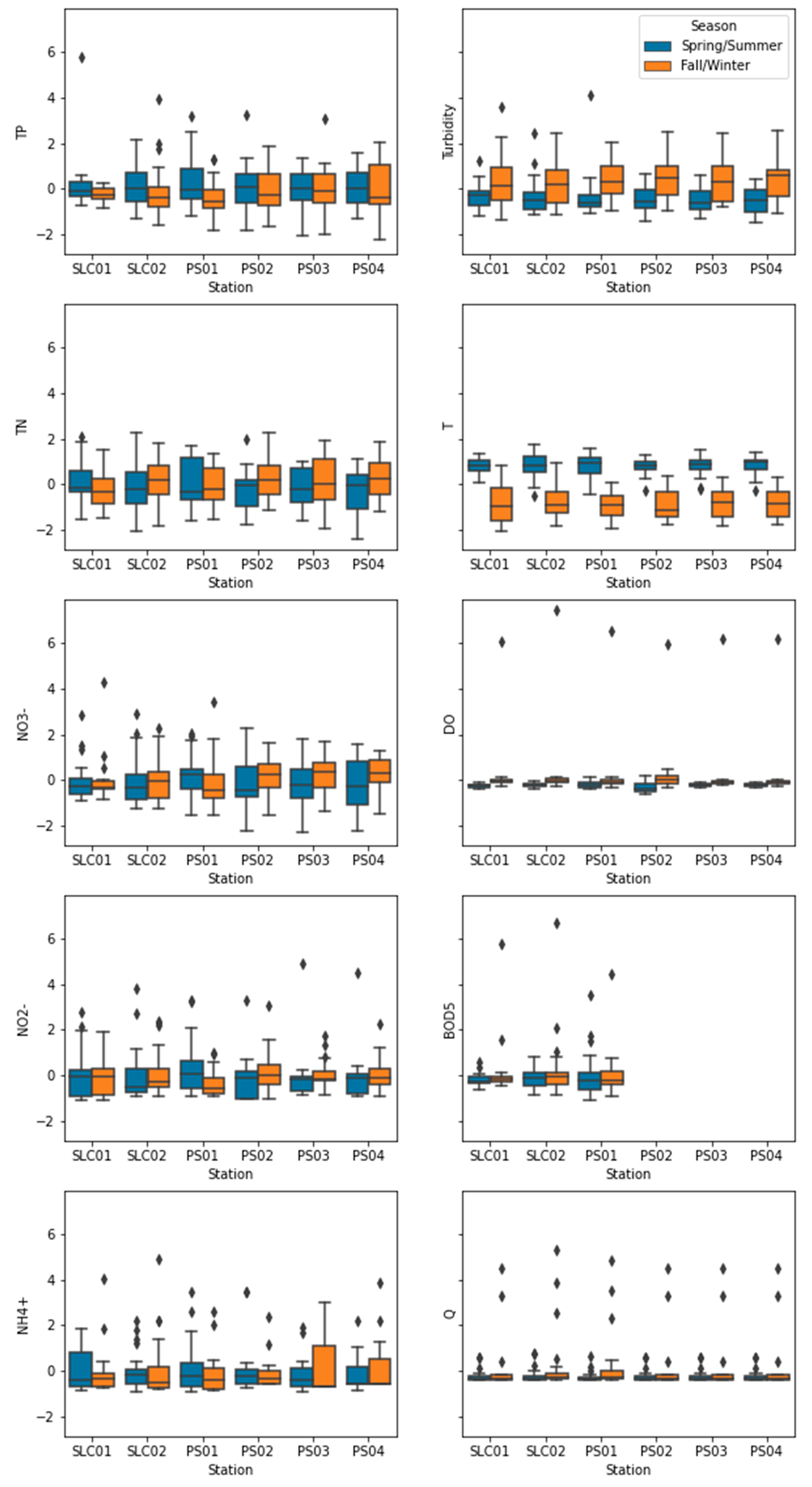
3.2.1. Temporal Trends

A k-means cluster analysis was conducted to assess the occurrence of temporal patterns in water quality at each water-quality monitoring station. For this purpose, ten attributes were considered (TP, TN, NO₃⁻, NO₂⁻, NH₄⁺, turbidity, T, DO, BOD₅, and Q), and each data point was labeled with the monitoring date of water-quality samples. Considering that the six monitoring sites are characterized by a different number of samples (n), six matrices (n × 11) were submitted to k-means, being n = 39 at SLC01, PS03, PS04, PS02; n = 63 at SLC02, and n = 51 at SLC03. Prior to classification, the attributes (ra-data) were mean-centered and scaled to unit variance to give equal importance to each attribute and handle their different measurement units. The k-means was applied to the first two dimensions (Dim). In Figure 5, the resulting spider plot obtained for SLC01 is shown as an example.

In Figure 5, it is possible to identify two different clusters: k1 or Winter Cluster, which includes water-quality observations that occurred in the fall and winter months (April–May–June–July–August–September); and k2 or Summer Cluster, which includes water-quality monitoring that occurred in spring and summer months (October–November–December–January–February–March). It is worth remarking that the month grouping used in this study is arbitrary. Therefore, the months April and October can be considered as “shoulder months,” which can belong to k1 or k2, depending on the arbitrary month grouping. This explains the presence of two April data points in the Summer Cluster. Similar results were obtained at the other five water-quality monitoring stations.

With the aim of thoroughly investigating the occurrence of temporal patterns and confirming or adding more information to the outcomes of the spider plot (Figure 5), seasonal (fall/winter and spring/summer) water-quality-parameter box-plots were used as a complementary tool (Figure 6). Furthermore, in this case, for a better comparison, row data were normalized (mean equal to zero and standard deviation equal to one) and plotted with the same range of the y-axis. In the Supplementary Materials, the statistical description of the normalized variables is reported (SM-4).

The boxplots in Figure 6 show that the seasonal median of most all the water-quality variables is quite similar at all monitoring stations. The main difference can be detected for turbidity and temperature variables, whose median significantly differ between the fall/winter and spring/summer season. Intuitively, the temperature is higher in spring/summer; on the contrary, turbidity is higher in fall/winter. The latter can be justified from the flow-boxplot that is characterized by more and higher outliers in fall/winter. This means that during this season, frequent extreme events occur and, along with higher soil humidity due to low temperature, cause a higher runoff and, therefore, a larger amount of detached and washed-off sediments.

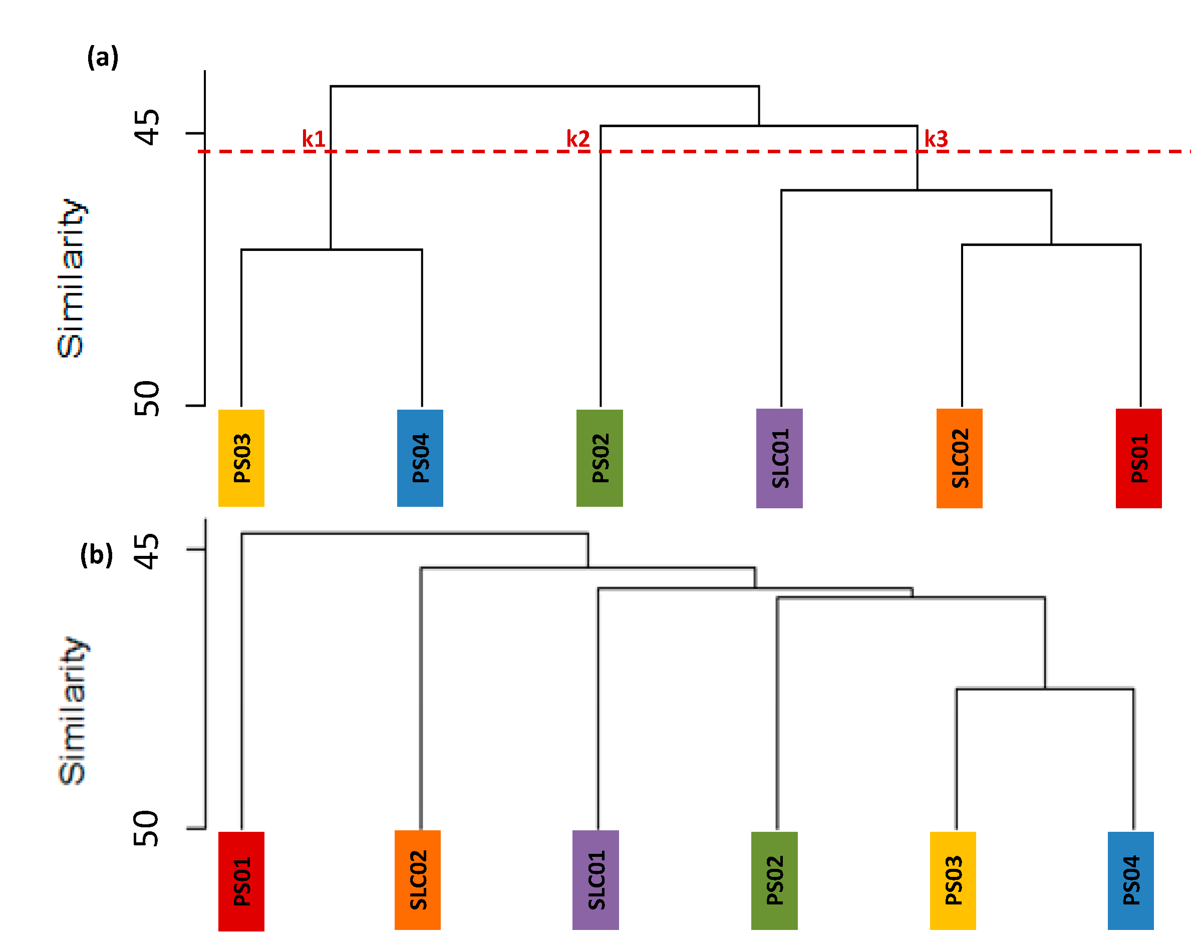
3.2.2. Spatial Similarity

HCA was applied to reveal spatial similarities among the water-quality monitoring sites. Based on the seasonal patterns previously identified, two data matrices (6 × 10) were the input for the HCA, being six the monitoring sites, nine the water-quality/hydrologic variables considered (TP, TN, NO₃⁻, NO₂⁻, NH₄⁺, turbidity, T, DO, and Q), and the last one was used as a label to identify the monitoring station. The two matrices were built considering the median of the seasonal observations (fall/winter and spring/summer) of each variable at each monitoring site. For this analysis, the variable BOD₅ was neglected due to the lack of its observations in three stations (PS03, PS04, and PS02). Moreover, in this case, each row-data input matrix was normalized. The resulting dendrograms obtained for the two seasons using Ward linkage and Euclidean distance are shown in Figure 7.

In Figure 7, it is possible to see that PS03 and PS04, the two monitoring stations located in the PS reservoir, are very similar from the water-quality point of view all year long. PS02, the most downstream station, comes immediately after. On the other side of the dendrograms, it is possible to identify the similarity that exists in spring/summer and fall/winter between PS01 and SLC02, which are two stations relatively close to each other, located immediately upstream PS reservoir. In Figure 7a, it is possible to identify three clusters (ki): k1 is formed by PS03 and PS04 (previously mentioned); k2 is composed by PS02, the monitoring station located at the outlet of the PS lake; k3 is characterized by SLC01, SLC02, and PS01, that represent the three monitoring stations located upstream the reservoir. This net cluster division is not visible in the spring/summer period (Figure 7b). This can be justified considering water balance as the driving force behind the pollutant transport at watershed scale. In particular, the fall/winter season is characterized by more frequent extreme events that, along with higher soil humidity, cause a higher runoff and, therefore, a larger amount of washed-off pollutants. This hypothesis is confirmed from the boxplots’ outcomes (Figure 6).

To provide an in-depth investigation of the spatial patterns of water-quality monitoring sites and confirm or add more information to the results obtained from the previous analysis (Figure 7), a PCA was run as a complementary analysis at each monitoring station. The dimension of the six input matrices was (n × 11), n being the number of water-quality samples (n = 39 at SLC01, PS03, PS04, PS02; n = 63 at SLC02, and n = 51 at PS01); ten attributes were considered (TP, TN, NO₃⁻, NO₂⁻, NH₄⁺, turbidity, T, DO, BOD₅, Q) and the last one, monitoring dates, were used as labels. Furthermore, in this case, this analysis was run on normalized matrices so that all attributes had zero mean and unit variance. The first four principal components (PCs) were selected, since they represented at least 70% of the total variance (69.0% at SLC01, 73.1% at SLC02, 69.7% at PS01, 82.7% at PS03, 80.2% at PS04, and 79.9% at PS02) and their eigenvalues are higher than one. The loadings outcomes obtained at each monitoring station are reported in

Table 4. Principal component (PC) loadings results at the six monitoring stations. Numbers in parenthesis represent the PC variance.

SLC01

PC1 (26.1%)

PC2 (20.3%)

PC3 (13.4%)

PC4 (12.4%)

SLC02

PC1 (33.3%)

PC2 (16.2%)

PC3 (13.1%)

PC4 (10.5%)

PS01

PC1 (32.1%)

PC2 (15.3%)

PC3 (13.1%)

PC4 (9.3%)

TP

−0.22

−0.08

0.10

−0.47

TP

0.23

0.47

−0.08

−0.48

TP

−0.44

0.05

−0.01

0.27

TN

−0.06

0.46

−0.48

−0.23

TN

−0.35

0.41

0.23

0.03

TN

−0.31

0.46

0.19

0.08

NO3−

0.05

0.41

−0.48

0.31

NO3−

−0.38

0.25

0.03

−0.20

NO3−

−0.15

0.39

−0.58

−0.05

NO2−

−0.07

0.29

0.00

−0.63

NO2−

−0.09

0.11

−0.67

−0.16

NO2−

−0.34

0.05

0.02

0.47

NH4+

−0.27

−0.41

−0.41

−0.26

NH4+

0.22

0.22

0.53

−0.42

NH4+

−0.34

0.24

0.29

0.14

Turbid.

0.45

0.22

0.12

0.03

Turbid.

−0.43

0.30

0.07

0.13

Turbid.

0.19

0.59

0.29

−0.16

T

−0.53

0.20

0.08

0.08

T

0.39

0.41

0.00

0.34

T

−0.41

−0.25

−0.01

−0.39

DO

0.48

−0.31

−0.08

−0.27

DO

−0.38

−0.34

0.03

−0.48

DO

0.35

−0.06

−0.09

0.70

BOD5

−0.09

−0.42

−0.49

0.21

BOD5

0.00

−0.28

0.46

0.13

BOD5

0.04

0.26

−0.65

−0.05

Q

0.38

0.05

−0.29

−0.17

Q

−0.37

0.17

0.05

0.38

Q

0.37

0.30

0.20

−0.09

PS03

PC1 (31.5%)

PC2 (21.1%)

PC3 (17.5%)

PC4 (12.6%)

PS04

PC1 (33.6%)

PC2 (21.3%)

PC3 (13.3%)

PC4 (12.0%)

PS02

PC1 (32.7%)

PC2 (20.0%)

PC3 (14.1%)

PC4 (13.1%)

TP

−0.26

0.15

−0.50

0.39

TP

−0.23

0.44

−0.42

0.23

TP

0.36

0.40

0.00

0.23

TN

0.09

0.59

0.35

−0.04

TN

0.34

0.37

0.19

−0.07

TN

−0.25

0.53

−0.07

−0.22

NO3−

−0.05

0.42

0.06

0.71

NO3−

0.12

0.38

−0.26

−0.70

NO3−

−0.06

0.62

−0.08

0.44

NO2−

0.33

−0.30

−0.44

0.06

NO2−

0.29

−0.10

−0.50

0.52

NO2−

−0.30

0.18

−0.36

−0.37

NH4+

−0.13

0.43

−0.24

−0.49

NH4+

−0.17

0.39

0.53

0.38

NH4+

0.01

0.30

0.45

−0.63

Turbid.

0.49

−0.11

−0.01

0.27

Turbid.

0.51

−0.13

−0.13

0.09

Turbid.

−0.55

0.05

−0.06

0.09

T

−0.51

−0.18

0.16

0.06

T

−0.51

−0.14

0.01

−0.01

T

0.46

0.01

−0.21

−0.39

DO

0.42

0.36

−0.31

−0.14

DO

0.32

0.41

0.21

0.16

DO

−0.17

−0.02

0.76

0.11

Q

0.34

−0.09

0.50

0.05

Q

0.28

−0.41

0.36

−0.09

Q

−0.41

−0.23

−0.16

−0.07

. Factor loadings help in understanding the basic nature of a component and are analogous to the correlation between original variables and PC. In this study, PC loadings above |0.5| were considered to have a major contribution to the associated factor [43] (highlighted in Table 4).

The PC loadings marked in Table 4 are not very high; therefore, it is not possible to find a clear spatial pattern. Consequently, a rotation of the PCs was carried out to get a more straightforward and appropriate depiction of the primary factors, by reducing the contribution of less significant variables. Rotation modifies the variance explained by each factor. Varimax rotation is adopted in this study to simplify the expression of the sub-space previously found with the factor analysis in terms of just a few significant items each. The actual coordinate system is unchanged; it is the orthogonal basis that is being rotated to align with those coordinates. As well as for the PCA, the first four VFs were considered. The factor loadings of the varimax-rotated components are presented in

Table 5. Varifactors (VF) loadings results at the six monitoring stations.

SLC01	VF1	VF2	VF3	VF4	SLC02	VF1	VF2	VF3	VF4	PS01	VF1	VF2	VF3	VF4
TP	−0.05	0.03	−0.09	0.98	TP	−0.22	−0.11	−0.02	0.01	TP	−0.08	−0.07	0.19	−0.05
TN	−0.09	0.22	−0.08	−0.01	TN	0.08	0.21	0.91	0.28	TN	−0.20	0.06	0.17	−0.08
NO3−	−0.09	−0.10	0.00	−0.03	NO3−	0.22	0.10	0.29	0.91	NO3−	−0.03	0.04	0.05	0.19
NO2−	−0.09	0.97	−0.09	0.03	NO2−	0.05	0.05	−0.02	0.04	NO2−	−0.06	−0.12	0.95	−0.01
NH4+	−0.01	−0.01	0.30	0.17	NH4+	−0.10	−0.08	0.02	−0.08	NH4+	−0.11	0.12	0.15	0.03
Turbid.	0.27	0.04	−0.12	−0.11	Turbid.	0.18	0.44	0.34	0.29	Turbid.	0.02	0.95	−0.12	0.01
T	−0.93	0.13	−0.04	0.07	T	−0.91	−0.03	0.01	−0.10	T	−0.34	−0.19	0.15	−0.10
DO	0.93	0.01	0.02	−0.01	DO	0.95	0.14	0.12	0.14	DO	0.93	0.01	−0.06	−0.01
BOD5	0.05	−0.09	0.95	−0.10	BOD5	0.04	0.01	−0.03	−0.02	BOD5	0.00	0.01	−0.01	0.98
Q	0.26	0.04	−0.01	−0.07	Q	0.13	0.94	0.19	0.08	Q	0.12	0.26	−0.06	−0.01
PS03	VF1	VF2	VF3	VF4	PS04	VF1	VF2	VF3	VF4	PS02	VF1	VF2	VF3	VF4
TP	−0.12	−0.23	0.18	0.05	TP	0.03	0.06	−0.13	−0.27	TP	−0.25	−0.07	−0.21	0.04
TN	0.18	0.15	0.21	−0.23	TN	0.25	0.13	0.12	0.06	TN	0.10	0.17	0.08	0.20
NO3−	0.05	−0.03	−0.07	−0.11	NO3−	0.07	−0.10	0.05	−0.08	NO3−	0.16	0.02	−0.10	−0.04
NO2−	0.25	0.05	−0.08	0.92	NO2−	0.03	0.95	0.22	0.02	NO2−	0.13	0.97	0.11	0.05
NH4+	0.07	−0.10	0.95	−0.07	NH4+	0.08	−0.14	−0.13	−0.09	NH4+	−0.07	0.05	−0.08	0.97
Turbid.	0.38	0.45	−0.18	0.29	Turbid.	0.24	0.32	0.83	0.27	Turbid.	0.74	0.35	0.35	0.01
T	−0.93	−0.10	0.05	−0.11	T	−0.59	−0.19	−0.49	−0.08	T	−0.93	−0.04	−0.13	0.09
DO	0.93	−0.01	0.16	0.18	DO	0.96	0.00	0.14	−0.01	DO	0.20	−0.07	0.03	0.13
Q	0.03	0.94	−0.09	0.03	Q	0.01	0.03	0.18	0.94	Q	0.23	0.12	0.93	−0.09

. Moreover, in this case, VF loadings above |0.5| were considered to have a significant contribution to the associated factor [14] and were highlighted in Table 5.

At all monitoring sites, VF1 strongly contributes to T and DO. Their VF loadings have opposite signs everywhere. This is justified by the fact that DO concentration in the surface water is affected by T and has both a seasonal and a daily cycle. Cold water can hold more DO than warm water. In the late fall and winter, when the water temperature is low, the DO concentration is high. In the late spring and summer, when the water temperature is high, the DO concentration is often lower. VF1 is also contributed by turbidity at PS02. VF2 can be explained mainly with NO₂⁻ and Q. Considering that NO₂⁻ is part of the dissolved inorganic nitrogen (DIN), its correlation with the streamflow is clear. VF3, instead, is mostly contributed to by both particle-bound and dissolved nitrogen, considering that the most significant variables at all monitoring sites are TN, NH₄⁺, turbidity, and Q. It is also contributed to by BOD₅ only at SLC01. VF4 can be mainly explained by the dissolved inorganic form of nitrogen. NO₃⁻, NH₄⁺, NO₂⁻, and Q are the primary contributors. Only at SLC01 does TP have a significant influence. It is worth remarking that the variables that influence almost all the VFs are turbidity and Q. In particular, turbidity affects VF1, VF2, VF3, while Q affects VF2, VF3, and VF4. This can be justified by considering the critical role of sediments and water balance in the pollutant wash-off process as the driving forces behind the pollutant transport at watershed scale. In any case, it is worth remarking that the lower the variance of a VF, the bigger the amount is of water-quality variables that represent that VF. This is the case of VF3 and VF4.

Furthermore, it is important to remark that, among the other variables, SLC01 is the only site where organic matter and phosphorus (BOD₅ and TP) have influence. This is mainly due to the significant percentage of forest that characterizes the contributing catchment (S1) of this site. As well, only at PS01, whose contributing basin is characterized by urban land use, do turbidity, TN, and NH₄⁺ have an effect.

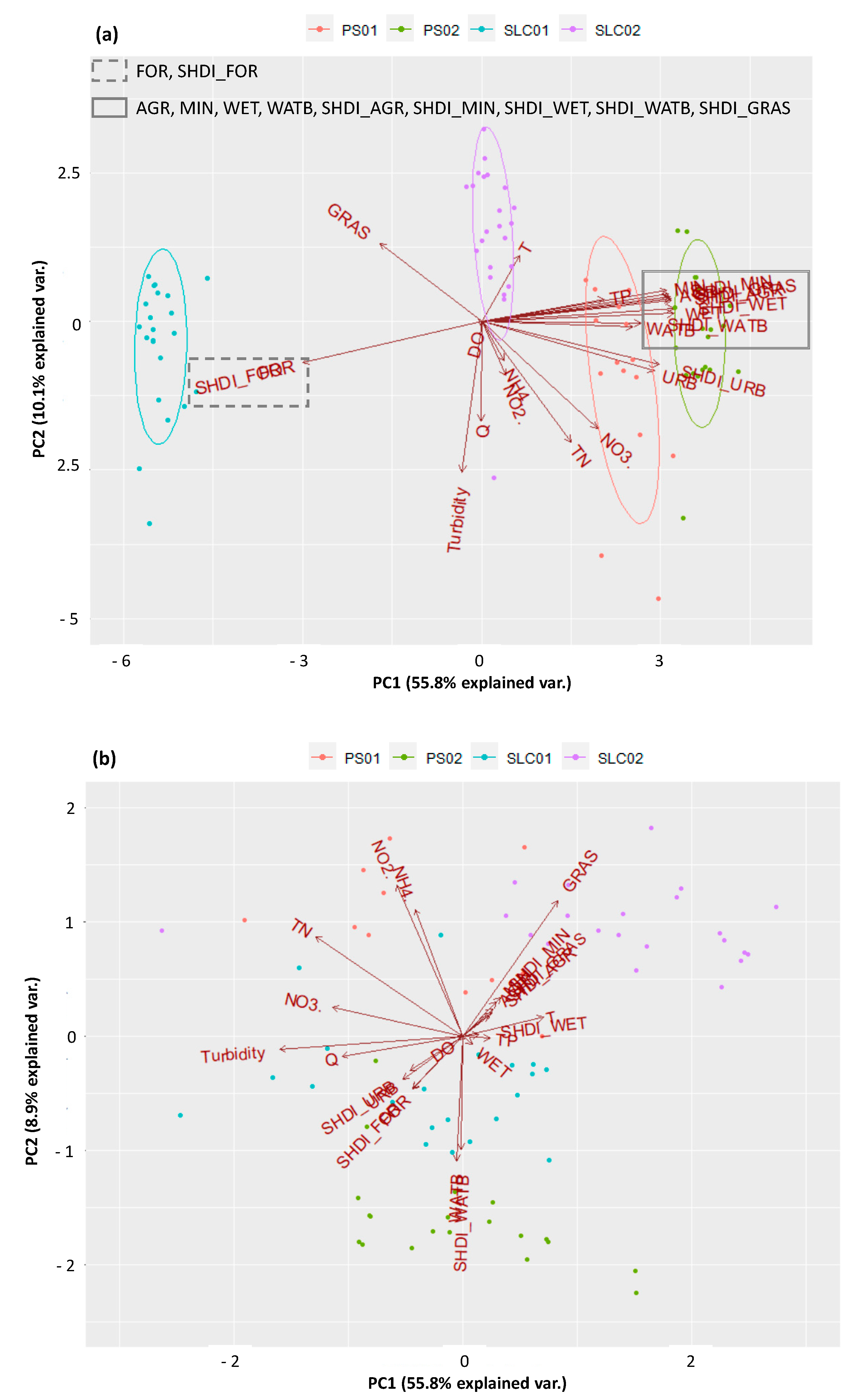
3.3. Relationship between Land Use and Water-Quality Variables

To assess whether there is a relationship between LULC and water-quality variables in the watershed, a PCA was undertaken as further analysis. Considering that the land use information available is from 2018, water-quality data from 2014 to 2018 were considered for this analysis, with the hypothesis that there were no land-use changes in these five years. A matrix (95 × 24) was submitted to PCA. The objects were the 95 water-quality samples, while the variables included the water-quality characteristics (9), the percentage of the LU/LC categories located in the contributing basins (7), the SHDI calculated for each land use type (7), and the last variable was used as a label to identify the monitoring stations (1). It is worth remarking that the four subcatchments considered for this analysis are the ones delineated in Figure 3 (S1, S2, S3, and S4). The first three PCs were selected, since they represented 75% of variance (PC1, PC2, and PC3 represent 55.8%, 10.1%, and 8.9% of the variance, respectively). In Figure 8, the resulting PCA biplots are shown.

The scores plot depicts the behavior of data points in the selected PCs and their similarities. In Figure 8a, the plane with the highest variance, the scores plot shows four well-defined groups, each of them includes data points of one of the four monitoring stations. Furthermore, it is interesting to notice that the four groups, from left to right, follow the order of the monitoring sites from upstream to downstream. Moreover, the distance between groups reflects the distance between the monitoring stations: SLC01 is the farthest, PS01, and PS02 are the closest since they are positioned where PS reservoir starts and ends, respectively.

The loadings plot analyzes the role of all the variables in the three PCs chosen, their relationships and their importance in the system. A remarkable outcome is represented by the strong correlation that exists between TP and agriculture-land use (AGR and SHDI_AGR). This is justified by the fact that most of the fertilizers used in Uruguay are phosphate-based [43]. Consequently, the import of fertilizers in the country was used as a proxy indicator of the agricultural intensification and it was found to be highly correlated with the TP measurements in the SL streamflow [18]. It is also worth mentioning that among the SLU categories related to agriculture, there is extensive cultivation in dairy farms (see SM-1 in the Supplementary Materials). This class includes intensive livestock farming that is known as one of the primary sources of nutrients to surface-water bodies [44,45]. In the land-cover classification used for this study, the category grassland mainly reflects extensive livestock farming. For this reason, a correlation between TP and SHDI_GRAS was also found. Moreover, in Uruguay, especially during the summer, it is common that stock directly accesses to waterways. This explains the strong correlation between nutrients and water-bodies vectors (WATB and SHDI_WATB). Consequently, in the SL watershed, since 2013, a strategic plan to control, stop and reverse the process of water-quality deterioration has been adopted [46]. In this plan, one of the management strategies is represented by the reduction of direct stock access to water bodies with fences.

Furthermore, in Figure 8, there exists an opposite correlation between TP and forest-land use. Soil nutrient levels within a watershed can decrease due to the uptake of bioavailable phosphorus by terrestrial vegetation. According to the age and type of vegetation, nutrient assimilation rates can vary. Forests are more effective in removing nutrients from basin soils, compared to shrubs and grassland, because of their foliage and more developed root system [47]. However, due to the low percentage of forested area, we believe that, in our case study, the vegetation contribution in reducing nutrient loads is not significant.

Another significant finding is represented by the robust correlation between nitrogen, in its dissolved (NO₃⁻, NO₂⁻, and NH₄⁺) and particle-bound (TN) form, and the urban vectors. Sources of nitrogen in urban areas include atmospheric deposition, wastewater effluent, lawn fertilizer application and leaky sewage infrastructure [48]. These sources differ from agricultural ecosystems where fertilizer is the dominant source of nitrogen, and, as we previously mentioned, the fertilizers mainly used in Uruguay are the phosphate ones. Another major result is given by the opposite correlation between GRAS vector (percentage of grassland–land use) and urban-related vectors. This relationship clearly represents the urbanization process that is occurring in the downstream part of SLC watershed: the city was built and reduced the area of the surrounding natural field.

It is also worth noting that forest-related vectors are located on the negative side of PC1, where SLC01-data points are located, as well as for urban, water bodies, and wetlands, that are close to PS01 and PS02-data points. The two grassland vectors are the only land-use vectors that are not very close to each other. This is due to the fact that grassland land-use type is the dominant one all over the watershed (Figure 4); therefore, the two vectors that represent the percentage of grassland land use and SHDI are closely located to the four subbasin data points.

Further outcomes can be highlighted in this analysis. There is a strong three-vector relationship among T, Q, and turbidity that is driven by T. The lower the T (winter season), the less influence the evapotranspiration process has, the more humid the soil is, and, consequently, the possibility of the occurrence of runoff volume with high energy able to detach and transport a significant amount of sediment to the river is higher. Another strong inverse correlation is represented by T and DO, as previously identified in Table 5: cold water (low T) can hold more DO than warm water (high T). Furthermore, the high phosphorus concentration that characterizes SLC-surface waters is almost independent from the turbidity measurement. This means that the inorganic dissolved form is the main form in which phosphorus can be detected in water (and not particle-bound). This outcome is in accordance with other studies carried out in the same watershed [18,49,50]. The presence of this phosphorus form in water, which is bioavailable, allows the growth of aquatic plants, microalgae, and cyanobacteria.

4. Conclusions

In this study, with the aid of multivariate exploratory analyses, we provided answers about the linkages between LU/LC types and the biophysical and chemical water-quality variables in the SLC watershed. This is a catchment characterized by a mixed land use, which leads to interfering with water-pollution generation, mobilization, and delivery to the superficial water bodies. The central outcomes of this study can be summarized in the following points:

• Trophic state. The TSI_stream shows a spatial increment of trophic state from upstream to downstream stations. Meanwhile, the TSI_lake shows hyper-eutrophic conditions in all PS-stations for the entire period (2011–2018). Higher TSI values are reported in the warm season. These results suggests that significant phosphorus concentrations are available to provide phytoplankton primary production in the middle-downstream part of the SLC watershed, particularly in the PS reservoir.
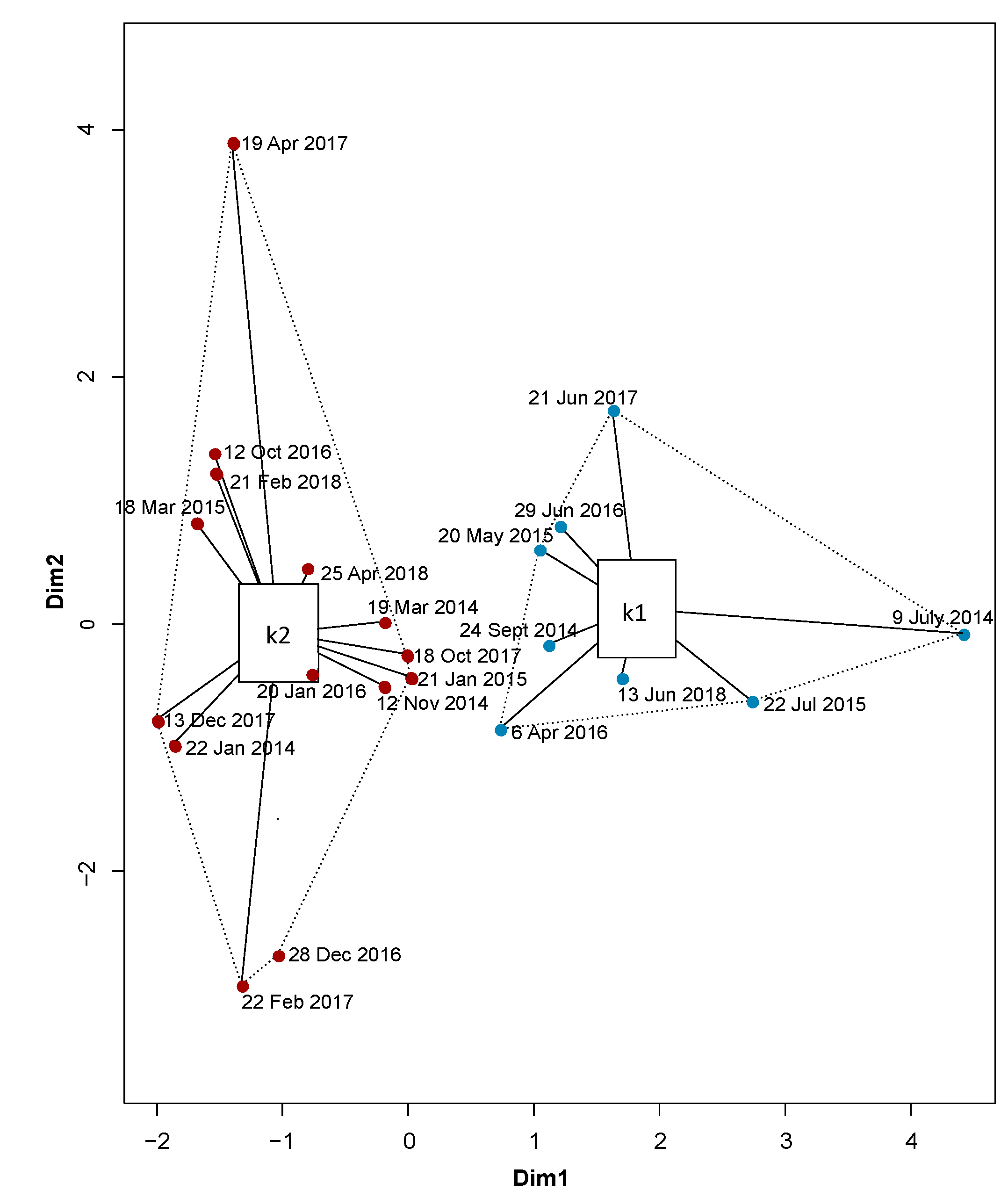
• Temporal and spatial patterns of water quality. From the temporal point of view, the PCA/k-means grouped the water-quality/hydrologic variables in two clusters representing spring/summer and fall/winter seasons. From the spatial point of view, the HCA identified spatial similarity in fall/winter period between PS03 and PS04, since they are located in the PS reservoir, and among SLC01, SLC02 and PS01, the three monitoring stations located upstream the reservoir.
• Primary water-quality variables. Turbidity and Q are the variables that have influence in almost all of the VFs. This can be justified considering the critical role of sediments and water balance in pollutant wash-off process, as the driving forces behind the pollutant transport at watershed scale. Furthermore, T and DO are characterized by an opposite correlation and are the two most significant variables in VF1 (characterized by the highest variance).
• Correlations LU/LC categories and water-quality variables. A strong correlation between TP and agriculture-land use was found. This is justified by the fact that most of the fertilizers used in Uruguay are phosphate-based. Furthermore, a clear correlation was found between nutrients (in particular, TP) and livestock farming. Even though the latter does not have a proper category, it was represented by the grassland–land cover (extensive livestock farming), the SLU agriculture category’s extensive cultivation in dairy farms (intensive livestock farming), and the water-bodies area (direct stock access to waterways). There also exists an inverse correlation between TP and forest-land use, due to the uptake of bioavailable phosphorus by vegetation. Nitrogen and urban-land use are highly correlated. Sources of nitrogen in urban areas include atmospheric deposition, wastewater effluent, lawn fertilizer application and leaky sewage infrastructure.

The outcomes of this work have proved that coupling large-scale studies and multivariate statistical methods can provide an appropriate overview of the water-quality behavior in space and time and relationships between water-quality variables and LU/LC. These findings represent adequate evidence for satisfactorily explaining in-stream water-quality variations related to current land use. Further investigation, along with an improved design of temporal and spatial sampling, may better describe the complex nature of the relationship between water quality and land use.

References

1. Xu, G.; Li, P.; Lu, K.; Tantai, Z.; Zhang, J.; Ren, Z.; Wang, X.; Yu, K.; Shi, P.; Cheng, Y. Seasonal changes in waterquality and its main influencing factors in the Dan River basin. Catena 2019, 173, 131–140. [Google Scholar] [CrossRef]
2. Calijuri, M.L.; de Siqueira Castro, J.; Costa, L.S.; Assemany, P.P.; Alves, J.E. Impact of land use/land cover changes on water quality and hydrological behavior of an agricultural subwatershed. Environ. Earth Sci. 2015, 74, 5373–5382. [Google Scholar] [CrossRef]
3. Wang, X.; Zhang, F. Effects of land use/cover on surface water pollution based on remote sensing and 3D-EEM fluorescence data in the Jinghe Oasis. Sci. Rep. 2018, 8, 13099. [Google Scholar] [CrossRef] [PubMed]
4. Liu, W.; Zhang, Q.; Liu, G. Influences of watershed landscape composition and configuration on lake-water quality in the Yangtze River basin of China. Hydrol. Process. 2012, 26, 570–578. [Google Scholar] [CrossRef]
5. Selle, B.; Schwientek, M.; Lischeid, G. Understanding processes governing water quality in catchments using principal component scores. J. Hydrol. 2013, 486, 31–38. [Google Scholar] [CrossRef]
6. Kändler, M.; Blechinger, K.; Seidler, C.; Pavlů, V.; Šanda, M.; Dostál, T.; Krása, J.; Vitvar, T.; Štich, M. Impact of land use on water quality in the upper Nisa catchment in the Czech Republic and in Germany. Sci. Total Environ. 2017, 586, 1316–1325. [Google Scholar] [CrossRef]
7. Miller, J.D.; Schoonover, J.E.; Williard, K.W.J.; Hwang, C.R. Whole catchment land cover effects on water quality in the Lower Kaskaskia River Watershed. Water Air Soil Pollut. 2011, 221, 337–350. [Google Scholar] [CrossRef]
8. Huang, J.; Zhan, J.; Yan, H.; Wu, F.; Deng, X. Evaluation of the impacts of land use on water quality. A case study in the Chaohu Lake Basin. Sci. World J. 2013, 2013, 329187. [Google Scholar] [CrossRef] [Green Version]
9. Shrestha, S.; Kazama, F. Assessment of surface water quality using multivariate statistical techniques: A case study of the Fuji river basin, Japan. Environ. Model. Softw. 2007, 22, 464–475. [Google Scholar] [CrossRef]
10. Zhou, T.; Wu, J.; Peng, S. Assessing the effects of landscape pattern on river water quality at multiple scales: A case study of the Dongjiang River watershed, China. Ecol. Indic. 2012, 23, 166–175. [Google Scholar] [CrossRef]
11. Xia, L.L.; Liu, R.Z.; Zao, Y.W. Correlation analysis of landscape pattern and water quality in Baiyangdian watershed. Procedia Environ. Sci. 2012, 13, 2188–2196. [Google Scholar] [CrossRef] [Green Version]
12. Kersebaum, K.C.; Steidl, J.; Bauer, O.; Piorr, H.-P. Modelling scenarios to assess the effects of different agricultural management and land use options to reduce diffuse nitrogen pollution into the river Elbe. Phys. Chem. Earth 2003, 28, 537–545. [Google Scholar] [CrossRef]
13. Azhar, S.C.; Aris, A.Z.; Yusoff, M.K.; Ramli, M.F.; Juahir, H. Classification of river water quality using multivariate analysis. Procedia Environ. Sci. 2015, 30, 79–84. [Google Scholar] [CrossRef] [Green Version]
14. Dutta, S.; Dwivedi, A.; Kumar, M.S. Use of water quality index and multivariate statistical techniques for the assessment of spatial variations in water quality of a small river. Environ. Monit. Assess. 2018, 190, 718. [Google Scholar] [CrossRef]
15. Namugize, J.N.; Jewitt, G.; Graham, M. Effects of land use and land cover changes on water quality in the uMngeni river catchment, South Africa. Phys. Chem. Earth 2018, 105, 247–264. [Google Scholar] [CrossRef]
16. Navas, R.; Alonso, J.; Gorgoglione, A.; Vervoort, R.W. Identifying climate and human impact trends in streamflow: A case study in Uruguay. Water 2019, 11, 1433. [Google Scholar] [CrossRef] [Green Version]
17. MVOTMA. Plan Nacional de Aguas. Montevideo, Uruguay. 2017. Available online: http://www.mvotma.gub.uy/politica-nacional-de-aguas/plan-nacional-de-aguas (accessed on 6 May 2020).
18. Aubriot, L.; Delbene, L.; Haakonson, S.; Somma, A.; Hirsch, F.; Bonilla, S. Evolución de la eutrofización en el Río Santa Lucía: Influencia de la intensificación productiva y perspectivas. Innotec 2017, 14, 7–17. [Google Scholar] [CrossRef]
19. Goyenola, G.; Meerhoff, M.; Teixeira-de Mello, F.; González-Bergonzoni, I.; Graeber, D.; Fosalba, C.; Vidal, N.; Mazzeo, N.; Ovesen, N.B.; Jeppesen, E.; et al. Phosphorus dynamics in lowland streams as a response to climatic, hydrological and agricultural land use gradients. Hydrol. Earth Syst. Sci. Discuss. 2015, 12, 3349–3390. [Google Scholar] [CrossRef]
20. INUMET. Uruguayan Institute of Meteorology. Available online: https://www.inumet.gub.uy/ (accessed on 6 May 2020).
21. DINAMA. OAN–Observatorio Ambiental Nacional. Available online: https://www.dinama.gub.uy/oan/geoportal/ (accessed on 4 May 2020).
22. DINAMA. Manual de Procedimientos Analíticos Para Muestras Ambientales. Available online: https://www.mvotma.gub.uy/index.php/component/k2/item/10009810-manual-de-procedimientos-analiticos-para-muestras-ambientales-tercera-edicion-2017 (accessed on 4 May 2020).
23. MGAP. Uruguayan Integrated Land Use/Land Cover Map. 2018. Available online: https://www.gub.uy/ministerio-ganaderia-agricultura-pesca/comunicacion/publicaciones/mapa-integrado-coberturauso-del-suelo-del-uruguay-ano-2018 (accessed on 4 May 2020).
24. DINAMA. Trophic State Index. Available online: https://www.dinama.gub.uy/oan/indicadores/ (accessed on 4 May 2020).
25. Andrietti, G.; Freire, R.; do Amaral, A.G.; de Almeida, F.T.; Carvalho Bongiovani, M.; Schneider, R.M. Índices de qualidade da água e de estado trófico do rio Caiabi, MT. Ambiente Água Interdiscip. J. Appl. Sci. 2015. [Google Scholar] [CrossRef]
26. Carlson, R. A trophic state index for lakes. Limnol. Oceanogr. 1977, 22, 361–369. [Google Scholar] [CrossRef] [Green Version]
27. Lamparelli, M.C. Degrees of Trophy in Water Bodies of São Paulo: Evaluation of Monitoring Methods. Ph.D. Thesis, Institute of Biosciences, University of São Paulo, São Paulo, Brazil, 2004. [Google Scholar]
28. Team, R.C. R: A Language and Environment for Statistical Computing; R Foundation for Statistical Computing: Vienna, Austria, 2017; Available online: https://www.R-project.org/ (accessed on 30 April 2020).
29. Jain, A.K.; Murty, M.N.; Flynn, P.J. Data Clustering: A Review. ACM Comput. Surv. 1999, 31, 264–323. [Google Scholar] [CrossRef]
30. Du, X.; Shao, F.; Wu, S.; Zhang, H.; Xu, S. Water quality assessment with hierarchical cluster analysis based on Mahalanobis distance. Environ. Monit. Assess. 2017, 189, 335. [Google Scholar] [CrossRef] [PubMed]
31. Gorgoglione, A.; Gioia, A.; Iacobellis, V. A Framework for assessing modeling performance and effects of rainfall-catchment-drainage characteristics on nutrient urban runoff in poorly gauged watersheds. Sustainability 2019, 11, 4933. [Google Scholar] [CrossRef] [Green Version]
32. Narbondo, S.; Gorgoglione, A.; Crisci, M.; Chreties, C. Enhancing Physical Similarity Approach to Predict Runoff in Ungauged Watersheds in Sub-Tropical Regions. Water 2020, 12, 528. [Google Scholar] [CrossRef] [Green Version]
33. Massart, D.L.; Vandeginste, B.G.M.; Deming, S.M.; Michotte, Y.; Kaufman, L. Chemometrics-A Text Book; Elsevier: Amsterdam, The Netherlands, 1988; Chapters 1–4; pp. 14–21. [Google Scholar]
34. Gorgoglione, A.; Bombardelli, F.A.; Pitton, B.J.L.; Oki, L.R.; Haver, D.L.; Young, T.M. Role of sediments in insecticide runoff from urban surfaces: Analysis and modeling. Int. J. Environ. Res. Public Health 2018, 15, 1464. [Google Scholar] [CrossRef] [Green Version]
35. He, Y.; Gao, B.; Sophian, A.; Yang, R. Coil-Based Rectangular PEC Sensors for Defect Classification. In Transient Electromagnetic-Thermal Nondestructive Testing; Elsevier: London, UK; New York, NY, USA, 2017; Chapter 4; pp. 55–90. ISBN 9780128127872. [Google Scholar]
36. Singh, K.P.; Malik, A.; Mohan, D.; Sinha, S. Multivariate statistical techniques for the evaluation of spatial and temporal variations in water quality of Gomti River (India)—A case study. Water Res. 2004, 38, 3980–3992. [Google Scholar] [CrossRef]
37. MVOTMA. Estado de Situación Cuenca del Río Santa Lucía. Montevideo. 2015. Available online: https://www.dinama.gub.uy/oan/documentos/Documento_Adjunto_1.pdf (accessed on 4 May 2020).
38. Liu, A.; DUodu, G.O.; Goonetilleke, A.; Ayoko, G.A. Influence of land use configurations on river sediment pollution. Environ. Pollut. 2017, 229, 639–646. [Google Scholar] [CrossRef]
39. Shi, P.; Zhang, Y.; Li, Z.; Li, P.; Xu, G. Influence of land use and land cover patterns on seasonal water quality at multi-spatial scales. Catena 2017, 151, 182–190. [Google Scholar] [CrossRef]
40. Ding, J.; Jiang, Y.; Liu, Q.; Hou, Z.; Liao, J.; Fu, L.; Peng, Q. Influences of the land use pattern on water quality in low-order streams of the Dongjiang River basin, China: A multi-scale analysis. Sci. Total Environ. 2016, 551–552, 205–216. [Google Scholar] [CrossRef]
41. Lee, S.W.; Hwang, S.J.; Lee, S.B.; Hwang, H.S.; Sung, H.C. Landscape ecological approach to the relationship of land use patterns in watersheds to water quality characteristics. Landsc. Urban Plan. 2009, 92, 80–89. [Google Scholar] [CrossRef]
42. Rigosi, A.; Carey, C.C.; Ibelings, B.W.; Brookes, J.D. The interaction between climate warming and eutrophication to promote cyanobacteria is dependent on trophic state and varies among taxa. Limnol. Oceanogr. 2014, 59, 99–114. [Google Scholar] [CrossRef] [Green Version]
43. MGAP. Datos Estadísticos de Importaciones de Fertilizantes. Dirección General de Servicios Agrícolas. 2016. Available online: http://www2.mgap.gub.uy/DieaAnterior/Anuario2015/DIEA-Anuario2015-01web.pdf (accessed on 4 May 2020).
44. Kato, T.; Kuroda, H.; Nakasone, H. Runoff characteristics of nutrients from an agricultural watershed with intensive livestock production. J. Hydrol. 2009, 368, 79–87. [Google Scholar] [CrossRef]
45. Yang, Q.; Tian, H.; Li, X.; Ren, W.; Zhang, B.; Zhang, X.; Wolf, J. Spatiotemporal patterns of livestock manure nutrient production in the conterminous United States from 1930 to 2012. Sci. Total Environ. 2016, 541, 1592–1602. [Google Scholar] [CrossRef] [PubMed]
46. GNA and SNA. Plan de Acción Para la Protección de la Calidad Ambiental de la Cuenca del Río Santa Lucía. Available online: http://mvotma.gub.uy/component/k2/item/10013640-plan-de-accion-santa-lucia-medidas-de-segunda-generacion (accessed on 15 May 2020).
47. Lintern, A.; Webb, J.A.; Ryu, D.; Liu, S.; Bende-Michl, U.; Waters, D.; Leahy, P.; Wilson, P.; Western, W. Key factors influencing differences in stream water quality across space. WIREs Water 2018, 5, 1260. [Google Scholar] [CrossRef] [Green Version]
48. Reisinger, A.J.; Groffman, P.M.; Rosi-Marshall, E.J. Nitrogen-cycling process rates across urban ecosystems. FEMS Microbiol. Ecol. 2016, 92, 198. [Google Scholar] [CrossRef]
49. Barreto, P.; Dogliotti, S.; Perdomo, C. Surface water quality of intensive farming areas within the Santa Lucia River basin of Uruguay. Air Soil Water Res. 2017, 10, 1–8. [Google Scholar] [CrossRef] [Green Version]
50. Chalar, G.; Garcia-Pesenti, P.; Silva-Pablo, M.; Perdomo, C.; Olivero, V.; Arocena, R. Weighting the impacts to stream water quality in small basins devoted to forage crops, dairy and beef cow production. Limnol. Ecol. Manag. Inland Waters 2017, 65, 76–84. [Google Scholar] [CrossRef]
Figure 1. Santa Lucía Chico (SLC) watershed with the location of the hydrometric station (red triangle), water-quality monitoring stations (black dots), and subcatchment delineation.
Sustainability 12 04692 g001
Figure 2. Primary land use (PLU) (top) and secondary land use (SLU) representation (bottom).
Sustainability 12 04692 g002
Figure 3. Subcatchments delineation based on water-quality monitoring sites.
Sustainability 12 04692 g003
Figure 4. Land use/land cover (LU/LC) percentage at each subcatchment (non-incremental).
Sustainability 12 04692 g004
Figure 5. Spider plot (k-means) of water-quality monitoring at SLC01: k1 represents the Winter Cluster (blue dots); k2 represents the Summer Cluster (red dots).
Sustainability 12 04692 g005
Figure 6. Seasonal variations (fall/winter and spring/summer) of water-quality parameters at the six water-quality monitoring sites.
Sustainability 12 04692 g006
Figure 7. Dendrogram to identify the spatial similarity of water-quality monitoring sites in SLC watershed in (a) fall/winter, (b) spring/summer.
Sustainability 12 04692 g007
Figure 8. Principal component analysis (PCA) land-use categories and water-quality variables: (a) PC1 vs. PC2, and (b) PC2 vs. PC3.
Sustainability 12 04692 g008