Sensitivity Analysis in Probabilistic Structural Design: A Comparison of Selected Techniques

Department of Structural Mechanics, Faculty of Civil Engineering, Brno University of Technology, 602 00 Brno, Czech Republic
Sustainability 2020, 12(11), 4788; https://0-doi-org.brum.beds.ac.uk/10.3390/su12114788
Submission received: 10 May 2020
/
Revised: 5 June 2020
/
Accepted: 5 June 2020
/
Published: 11 June 2020
(This article belongs to the Special Issue Sustainable Construction Engineering and Management)
Abstract
:Although more and more reliability-oriented sensitivity analysis (ROSA) techniques are now available, review and comparison articles of ROSA are absent. In civil engineering, many of the latest indices have never been used to analyse structural reliability for very small failure probability. This article aims to analyse and compare different sensitivity analysis (SA) techniques and discusses their strengths and weaknesses. For this purpose, eight selected sensitivity indices are first described and then applied in two different test cases. Four ROSA type indices are directly oriented on the failure probability or reliability index beta, and four other indices (of a different type) are oriented on the output of the limit state function. The case study and results correspond to cases under common engineering assumptions, where only two independent input variables with Gaussian distribution of the load action and the resistance are applied in the ultimate limit state. The last section of the article is dedicated to the analysis of the different results. Large differences between first-order sensitivity indices and very strong interaction effects obtained from ROSA are observed for very low values of failure probability. The obtained numerical results show that ROSA methods lack a common platform that clearly interprets the relationship of indices to their information value. This paper can help orientate in the selection of which sensitivity measure to use.
1. Introduction
Evaluating the reliability of building structures is a problem whose final goal remains a decision-making process [1]. In a probabilistic framework, the basic characteristic of engineering reliability is the probability of failure Pf, which represents the key quantity of interest in decision-making processes [2]. It is recommended by the best practices that such a report is supplemented with sensitivity analysis (SA), which describes the effect of changes in model inputs on the measure of reliability [3].
A classical measure of change in Pf is the derivative ∂Pf/∂μxi with respect to the mean value μ of input variable Xi [4,5,6,7]. A drawback of the derivative-based SA is that it cannot detect interactions between input variables. Since only one μxi is varied at a time while others are fixed, it can be labelled as the One-At-a-Time (OAT) method or local SA (at point μxi). The aforementioned drawback can partially be overcome by using the factorial experiment, where SA is computed using two-level changes of μxi for all Xi in combinations, which permit the computation of interaction effects [8]. However, only absolute change of the distribution parameter μxi on Pf is investigated, not the relative influence of the random variability of Xi on Pf. For structural reliability, it is better to prefer such SA types that can compute the effects of the random variabilities of input variables and their interactions on Pf and not just changes in distribution parameters.
Compared with the local SA, global SA [9] can measure the effect of input variables on the model output in their entire distribution ranges and provide the interaction effect among different input variables. In the literature, many global SA techniques, such as the non-parametric techniques [10], screening approaches [11], Sobol’s variance-based (ANOVA) methods [12,13] and moment-independent methods [14,15], can be found, among which the variance-based method has gained the most attention. Variance is an important component of reliability analysis, but is insufficient on its own for the analysis of structural reliability; see, for e.g., [16]. A more general approach, which generalized Sobol’s sensitivity indices, was introduced by Fort et al. [17]. These indices are generally applicable (goal-oriented) because they can analyze various key quantities of interest, including Pf.
The selection of SA methods that focus on Pf or design quantiles is usually based on a stochastic model with binary output failure/nonfailure, 1/0 [18], but it is not a necessity. In first-order reliability method (FORM), Pf can be replaced by reliability index β [19], which is computed using the first two moments of resistance, and load action and can be applied as an alternative measure of reliability; see Figure 1. However, global SA of β has not yet been developed.
From a computational point of view, probabilistic sensitivity measures have been comprehensively studied; however, from a decision-analytic point of view, they remain much less understood [20]. Their relationship to information value has not yet been particularly established. Linking the information value, SA, and forecasting with scoring rules remains a subject of research [20]. For a particular reliability task, it is necessary to look for means to select the most appropriate sensitivity measure with common rationale for this selection.
In civil and construction engineering, the scientific community uses SA in structural mechanics [21,22], geotechnics [23,24], landscape water management [25], building performance analysis [26], multi-criteria decision making (MCDM) [27], sustainable development of the building sector [28] or sensitivity audits to assess sustainability [29], but with a lower publication frequency than in basic sciences, such as chemistry, economics or mathematics [30]. In structural reliability, research deals with limit states [31] or the verification of partial safety factors of Eurocode standards [32] using various types of global SA based, for example, on the variance of model outputs [33,34].
The term “sensitivity analysis” can be understood differently in civil engineering than in basic sciences, where local and global SA types with random inputs are well established. For example, very specific (non-stochastic) SA methods based on advanced non-linear models are sometimes used for structures susceptible to buckling when the subject of interest is the stability (or potential energy) of structures [35,36] or imperfection sensitivity [37,38], whereby the main objective of these methods is to increase the stability limits of the structures through the variation of suitable design variables. In stochastic systems, stability often means insensitivity or low sensitivity of the output characteristics to the shapes of some input distributions [39]. In construction engineering, it is necessary to focus more on cooperation and integration of SA development [3] with reliability analysis tools [31,40] and decision-making processes [41,42].
This paper compares several existing sensitivity measures in the context of structural reliability in civil engineering. For this purpose, eight selected sensitivity indices are first described and then applied in two different test cases.
Four indices are oriented on the probability of failure or reliability index β, another four on the distribution or some moments of the output from the ultimate limit state function Equation (2). The reason for the inclusion of the second group of indices is their common use in the analysis of limit states, despite being only sensitive to reliability; see, for e.g., [43,44]. Correlations present a typical example; however, sensitivity techniques based on fuzzy probability analysis of constructions [45,46] are no exception. These alternative types of SA are not directly focused on the probability of failure, but they provide basic insight into the behaviour of computational models, their structures and their reactions to changes in model inputs.
The presented article deals with four ROSA type SA and four other SA, which are empathetic to reliability in civil engineering. Special attention is paid to small failure probabilities, which are relevant for assessing the engineering reliability of structures using design reliability conditions.
2. Design Reliability Conditions
In limit state design, the resistance of a structure R must be greater than the load action F with a predetermined probability [19]. Structural reliability can also be assessed by comparing the lower quantile of R with the upper quantile of F [19], where the quantiles represent alternative key quantities of interest. The decision-maker who develops or implements stochastic models is expected to provide a forecast of structural reliability, which can be performed by estimating the failure probability, quantiles or other computational statistics related to limit states of structure.
Let the reliability of building structures be a one-dimensional random variable Z, which is a function of random variables.
The reliability assessment of load-bearing structures is based on a semi-probabilistic approach of standard [19], which falls into the category of FORM methods [47]. Structural reliability is often expressed as a limit state function of random resistance R and random load action F:
where R and F are statistically independent variables for which Gauss probability density functions (pdfs) are assumed with mean values μR, μF and standard deviations σR, σF. If R and F have Gauss pdfs, then Z has a Gauss pdf with mean value μZ and standard deviation σZ:
The transformation of Z into a normalized Gaussian pdf of U with mean value μU = 0, and standard deviation σU = 1 is written as
The probability of failure (key quantity of interest) can be expressed as
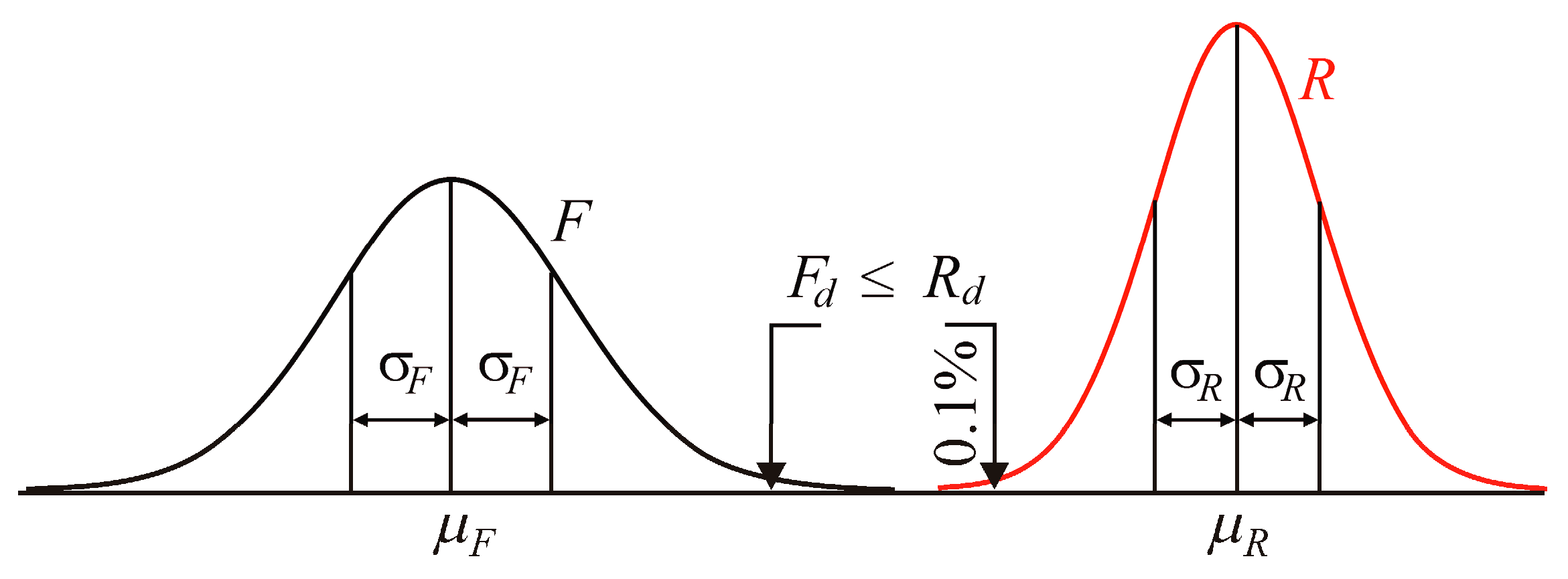
where ΦU(•) is the cumulative distribution function of normalized Gaussian pdf and μZ/σZ is the so-called reliability index β; see Equation (7) and Figure 1.
It is assumed that β > 0. Standard [19] verifies reliability by comparing the obtained reliability index β with the target reliability index βd.
For instance, the reliability index has a target value of βd = 3.8 (Pfd = 7.2·10−5), provided that we consider the ultimate limit state for common design situations within the reference period of 50 years; see Table C2 in [19] or [48]. Equation (8) can be written to obtain σZ as
where αF, αR are values of sensitivity coefficients (weight factors) according to the FORM method, which [19] introduces with constant values αF = 0.7, αR = 0.8. Substituting Equations (3) and (8) into Equation (7), we can write
Equation (9) is the design reliability condition with formally separated random variables that can be expressed as
where the left-hand side represents the design load Fd and the right-hand side the design resistance Rd; see Figure 2. The basic reliability targets for design values in the ultimate limit state recommended in [19] are based on the semi-probabilistic approach in Figure 2, with the target value of reliability index βd = 3.80 for a 50 years reference period [48,49]. For βd = 3.8, Rd can be approximately computed as 0.1 percentile [40]. Standard [19] enables the determination of design values Fd, Rd not only from a Gauss pdf but also from a two- or three-parameter lognormal (for resistance) or Gumbel or Gama (for load) pdfs. The probability of failure for non-Gaussian R and F can be estimated using Monte Carlo (or quasi-Monte Carlo) methods.
3. Selected Types of Sensitivity Analysis Methods
In reliability engineering, SA methods quantify the effects of input variables on the failure probability, reliability index β or design quantiles. However, other statistical model-based inferences sensitive to reliability are often used. In this chapter, we present selected formulae of selected types of sensitivity measures in forms that are adapted to structural reliability analysis.
Cramér–von Mises indices [50]. Input random variables in Equation (1) are assumed to be statistically independent. Let ΦZ be the distribution function of Z:
and is the conditional distribution function of Z conditionally on Xi:
The first-order Cramér–von Mises index Gi is based on measuring the distance between probability ΦZ(t) and conditional probability (t) when an input is fixed [50].
The second-order Cramér–von Mises index Gi can be expressed, on the basis of [50], as
where is the conditional distribution function of Z conditionally on Xi, Xj, for i < j:
Integration Equation (13) and Equation (14) respect t. Equation (13) is not oriented to one failure probability value Pf, but, depending on t, integrates the averages of squared values from the differences of all probabilities Equations (11) and (12) normalized by F(t)(1 − F(t)). The same applies to other higher-order indices [50]. Indices Gi, Gij, etc., are based on Hoeffding decomposition; therefore, the sum of all indices is equal to 1 [50]. It can be noted that Cramér–von Mises indices can be formulated in copula theory framework [51].
Sensitivity indices subordinated to contrasts associated with probability [17] (in short, Contrast Pf indices). These indices measure the distance between probability Pf and the conditional probability Pf|Xi using the contrast function in Equation (16). The input random variables in Equation (1) are assumed to be statistically independent.
The first-order probability contrast index Ci is defined as Equation (17), where the contrast is computed for probability estimator θ* = Argmin ψ(θ) = Pf.
The second term in the numerator in Equation (17) is computed as the average value of the conditional contrast functions whose probability estimator is Pf|Xi. The second-order probability contrast index Cij can be expressed as
where i < j. Indices of the third and higher orders are computed similarly [17]. Sensitivity indices subordinated to contrasts are based on decomposition; therefore, the sum of all indices must be equal to one. Examples of the computation of indices using the Latin Hypercube Sampling method (LHS) [52,53] in engineering applications are in [54,55].
Sensitivity indices subordinated to contrasts associated with α-quantile [17]. The contrast function ψ associated with α-quantile can be written with parameter θ as [17]:
where the input random variables in Equation (1) are assumed to be statistically independent. The first-order quantile contrast index Qi is defined as
where is the contrast computed for the estimator of α-quantile θ* = Argmin ψ(θ).
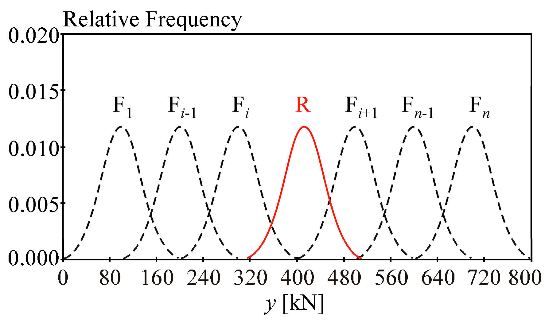
The second-order quantile contrast index Qij is defined as Equation (21), where i < j. Indices of the third and higher orders are computed in a similar manner [17]. Sensitivity indices subordinated to contrasts are based on decomposition; therefore, the sum of all indices must be equal to one. In engineering applications, the random variable Y is, for example, the load action F or resistance R [56]; see Figure 1.
Borgonovo moment independent importance measure [14] (in short, Borgonovo indices). The sensitivity indices described in [14] are defined by introducing a moment-independent uncertainty indicator that looks at the entire input/output distribution and whose definition is well-posed also in the presence of correlations among the input parameters.
where ϕZ(z) is the pdf of Z and ϕZ│Xi(z) is the conditional pdf of Z given that one of the parameters, Xi, assumes a fixed value [14]. Fixing pairs Xi, Xj, leads to the second-order index Bij, where i < j. Fixing triplets Xi, Xj, Xk leads to the third-order index Bijk, where i < j < k, etc. The sum of all indices is not equal to one. As a general rule, 0 Bi Bij.. B1,2,…,M 1 [14].
Reliability sensitivity index defined by Xiao et al. [57] (in short, Xiao indices). All the input variables are independent of each other. The first-order index Si measures the individual effect of Xi on Pf.
where |Pf – Pf|Xi| measures the absolute difference between the unconditional failure probability Pf and the conditional failure probability Pf|Xi. The second-order interaction indices Kij, where , are asymmetrical:
Reliability sensitivity index defined by Ling et al. [58] (in short, Ling indices). The first-order index is the same as in Equation (23) Li = Ki. Fixing pairs Xi, Xj, leads to the second-order index Lij, where i < j:
Fixing triplets Xi, Xj, Xk leads to the third-order index Lijk, where i < j < k, etc. The sum of all indices defined by Ling et al. [58] is not equal to one. As a general rule [58], 0 Li Lij... L1,2,…,M 1.
Sobol’s sensitivity indices [12,13] (in short, Sobol’s indices). Sobol’s first-order sensitivity indices can be written in the form:
where corr is Pearson correlation coefficient. Fixing pairs Xi, Xj, leads to the second-order index Sij, where i < j. Fixing triplets Xi, Xj, Xk leads to the third-order index Sijk, where i < j < k, etc.; see, for example [9]. The sum of all indices is equal to one. It can be noted that Sobol’s indices present a special case of sensitivity indices subordinated to contrasts in which the contrast function is associated with variance ψ(θ) = E(Z − θ)2 [17].
Omission sensitivity factor [59] (in short, Madsen’s factor). The omission sensitivity factor Oi is defined as the ratio between the conditional reliability index β|Xi = μxi and the reliability index β (7).
Random variable Xi is fixed at its mean value μxi in the numerator in Equation (27), but the possibility of fixing at the characteristic value [60] or median [3] is also indicated.
The indices described above can be divided into two groups. The first group (Sobol, Borgonovo and Cramér–von Mises) focuses on the distribution or some moments of the output function Z, while the second group (Xiao, Ling, Contrast, Madsen’s) considers Pf, β or quantiles as the quantity of interest and thus can be referred to as reliability analysis indices. The first group can be classified as global SA, while the second group can be classified as reliability-oriented sensitivity analysis (ROSA) [3], of which Xiao, Ling and Contrast indices can terminologically [54,57,58] be classified as global ROSA. It can be noted that Xiao, Ling and Contrast ROSA indices are typical examples of ambiguous “local–global” indices [3]. On one hand, they can be considered as global since they are based on changes of Pf with regard to the variability of the inputs over their entire distribution ranges and they provide the interaction effect between different input variables. On the other hand, they can be considered as local in the sense of regional SA since they are based on the frequency of failures from the random realization in “region” of pairs of large load actions and small resistances.
Correlations. The last SA methods used are the analysis of the correlation between the input Xi and output Z according to Pearson, Spearman and Kendal Tau.
4. Case Studies
Many new sensitivity indices have been developed, but their ability in applications has not yet been reliably demonstrated. In this article, the properties of the selected sensitivity indices mentioned in Chapter 3 are examined in a case study of the probabilistic analysis of the reliability of a steel bar under axial tension; see Figure 3. A static time-independent study is considered.
In general, the random load action F and resistance R are usually described using appropriate types of distribution functions ΦF(y), ΦR(y) and corresponding pdfs ϕF(y), ϕR(y), where y denotes a general point of the observed variable (force with the unit of Newton), through which both variables F and R are expressed; see right part of Figure 3. It is assumed that F and R are statistically independent of each other with mean values μF, μR and standard deviations σF, σR.
The probability of failure can be computed as the integral:
In the case studies, integration in Equation (28) is performed numerically by Simpson’s rule, using more than ten thousand integration steps over the interval [μZ − 10σZ, μZ + 10σZ].
Reliability can be assessed by comparing the computed Pf in Equation (6) with the target value of Pf, where target values for design cases are listed in standard EN1990 [19]. Target values of Pf in Table 1 are taken from Table B2 in [19]. Table 1 lists the minimum values of Pf (the reliability index β) for ultimate limit state and 50 years reference period. The description of subsequent classes RC1, RC2, and RC3 with examples of building and civil engineering works are in [19,48].
The aim of the presented study is the SA of the influence of input factors R, F on the output Pf using different types of sensitivity indices and the subsequent comparison of obtained results. Resistance R is the input random variable X1, and load action F is the input random variable X2.
4.1. Computation of Sensitivity Indices
This section includes a description of numerical methods for computing the size of sensitivity indices based on numerical integration methods in combination with sampling-based methods or analytical computation. Sensitivity indices were computed for eight SA types.
Contrast Pf indices [17] (ROSA). The contrast function Equation (16) is minimum if θ* = Pf. By substituting Pf into Equation (16), we can write first-order index in Equation (17) using = Pf (1 − Pf), and similarly for Pf|Xi, we can write = (Pf |Xi)(1 − (Pf |Xi)).
By substituting Pf (1 − Pf) and (Pf|Xi)(1 − (Pf|Xi)) into Equation (17), we can derive Equation (29) for practical use. Ci measures, on average, the effect of fixing Xi on Pf. The estimate of Pf is computed as the integral Equation (28). In the first loop, the estimate of Pf|Xi = P((Z|Xi) < 0) is computed by numerical integration across z∈[μZ − 10σZ, μZ + 10σZ]. In the second loop, E[•] is computed by numerical integration of the pdf of Xi with a small step Δxi taken over [μXi − 10σXi, μXi + 10σXi]. Since the second term in the numerator in Equation (18) is always equal to zero (Pf|X1,X2 is always equal to zero or one), C12 = 1 − C1 − C2.
Xiao indices [57] (ROSA). Indices K1, K2 are estimated from Equation (23) using double-nested-loop computation. In the outer loop, E[•] is computed by numerical integration of the pdf of Xi with a small step Δxi taken over [μXi − 10σXi, μXi + 10σXi]. Note: the estimate E[•] obtained using the LHS method would be inaccurate because it requires an extremely high number of runs for small values of Pf. In the nested loop, estimates of Pf and Pf|Xi are computed by integrating according to Equation (28). Indices K12 and K21 defined in Equation (24) are computed in a similar manner.
Ling indices [58] (ROSA). By definition, L1 = K1, L2 = K2. The computation of L12 includes an estimate of E[•], which is based on double numerical integration. In the outer loop, the pdf of X2 is numerically integrated with a small step Δx2 taken over [μX2 − 10σX2, μX2 + 10σX2]. In the inner loop, the pdf of X1 is numerically integrated with a small step Δx1 taken over [μX1 − 10σX1, μX1 + 10σX1]. During integration, the term Pf|X1,X2 can only have a value of 0 or 1.
Cramér–von Mises indices [50]. Indices G1 and G2 are computed using Equation (13). Three nested loops are applied. In the first (outer) loop, numerical integration is computed with a small step Δt = tl+1 − tl, where t = (tl+1 + tl)/2, t∈[μZ − 10σZ, μZ + 10σZ], l = 1, 2,..., 10000. To each Δt belongs dΦ(t)≈P(tl Z tl+1) and Φ(t)≈P(Z (tl+1 + tl)/2). In the second loop, E[•] in the numerator in Equation (13) is computed by numerical integration of the pdf of Xi with a small step Δxi taken over [μXi−10σXi, μXi+10σXi]. Note: The LHS estimation of E[•] would be numerically very challenging but is possible. In the third (deep) loop, Φi(t)≈P(Z (tl+1 + tl)/2|Xi = ξi) is computed by numerical integration for fixed ξi, where ξi is the middle of interval Δxi from the second loop. The index G12 is computed on the basis of Equation (14) in a similar manner.
Borgonovo indices [14]. Indices B1, B2 are estimated from Equation (13) using double-nested-loop computation. In the outer loop, 0.5·E[•] is computed using one million runs of the LHS method. In the nested loop, numerical integration |ϕZ(z) – ϕZ|Xi(z)| is taken over [μZ − 10σZ, μZ + 10σZ] using ten thousand runs. B12 = 1 in all case studies.
Sobol’s indices [12,13]. Sobol’s sensitivity indices are included only for comparison; these indices analyse the influence of the variance of R or F on the variance of Z, but not the influence on Pf. Sobol’s indices are computed analytically as S1 = /(), S2 = /(), S12 = 0. It can be noted that Sobol’s first-order indices are equal to the squares of the sensitivity coefficients (weight factors) in Equation (8): S1 = , S2 = .
Correlations. Correlation corr(X1, Z) and corr(X2, Z) are evaluated even though direct sensitivity to Pf is not measured by correlation. Pearson, Spearman and Kendal Tau correlation coefficients between input Xi and output Z are computed using one hundred thousand runs of the LHS method.
All E[•] are computed by numerical integration with the exception of Borgonovo indices and correlation. It can be noted that E[•] in the formulae in chapter 3 can also be numerically computed using Monte Carlo- (or quasi-Monte Carlo-) type simulation methods; however, the repeated computation of small values of Pf requires extremely high numbers of simulation runs and is numerically challenging.
4.2. Case Study 1
The aim of SA is to assess the influence of R and F on Pf. Let R (resistance) and F (load action) be statistically independent variables X1, X2 with Gauss pdfs, where μR = 412.54 kN, σR = 34.132 kN, σF = 34.132 kN, and mean value μF is the parameter; see Figure 4. Let parameter μF change with the step ΔμF = 10 kN and gradually attain the values 92.54 kN, 102.54 kN,..., 722.54 kN. The sensitivity indices are plotted in dependence on Pf, where Pf = ΦU(−(412.54 − μF)/(20.5·34.132)) is a function only of parameter μF. If μF decreases, then Pf decreases.
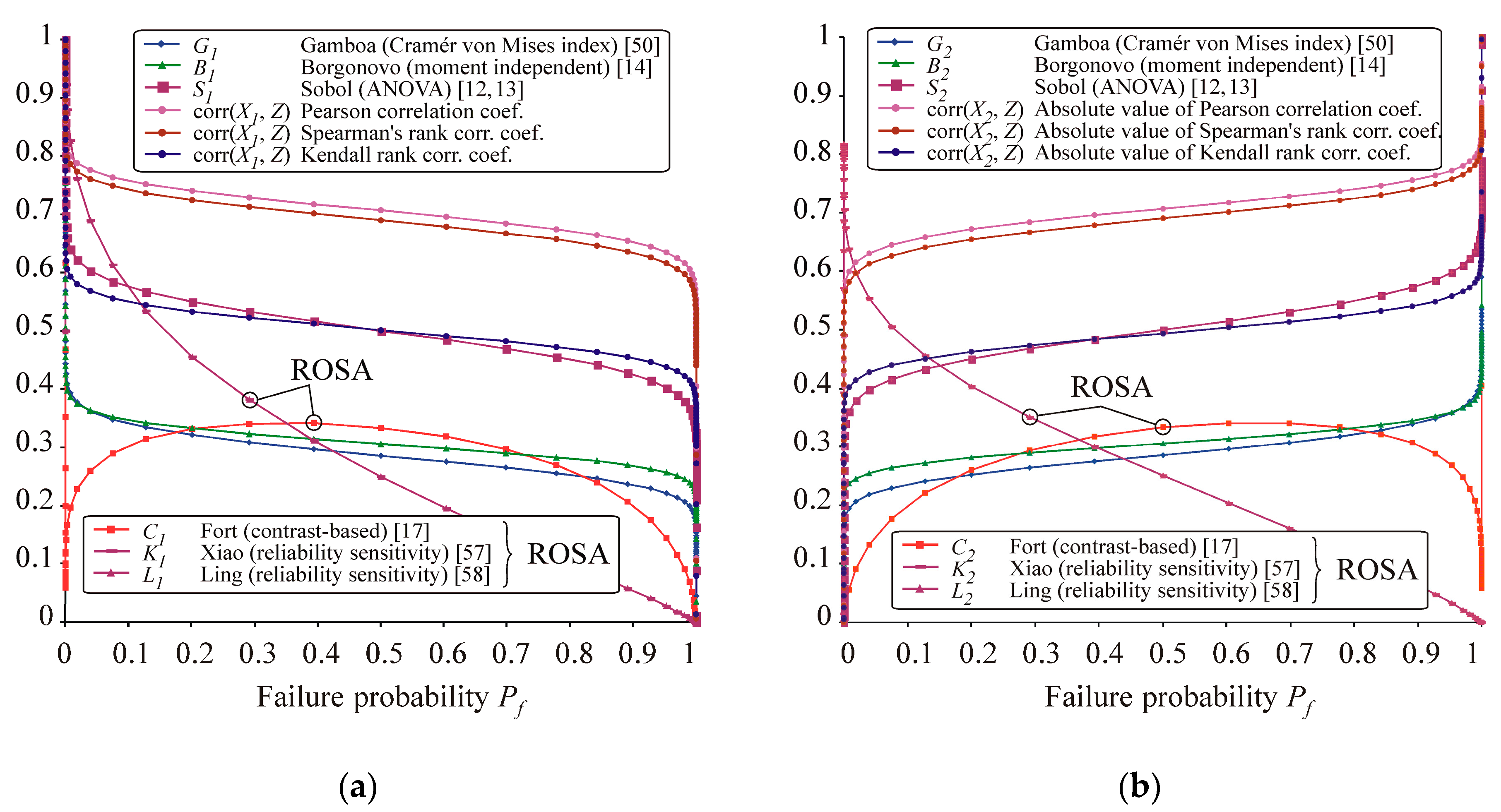
First-order indices are depicted in Figure 5 and the second-order indices are depicted on the left part of Figure 6. Correlation coefficients corr(X1, Z) and corr(X2, Z) are added to Figure 5. Only indices within the interval [0, 1] are depicted. Madsen’s factors are not plotted because they have a constant value O1 = O2 = 1.415 for all Pf (μF).
Changing Pf (μF) influences only indices C1, C2, C12, indices K1, K2, K12, K21 and indices L1, L2, L12; see Figure 5 and the left part of Figure 6. For the other five types of SA, it was observed that two variables that have a different influence on the output have the same indices. This demonstrates properties of sensitivity indices that will prove useful in the interpretation of the result.
Ling and Xiao indices are the only indices with asymmetric plots and decrease with increasing Pf. Xiao asymmetrical interaction indices are identical: K12 = K21. Contrast-based sensitivity indices have values of C1 = C2 = C12 = 0.33 for Pf = 0.5, but, otherwise, decrease with absolute distance from Pf = 0.5. Approaching Pf → 0 or Pf → 1 leads to C1 = C2 → 0 and C12 → 1. Change in mean value μF has no influence on the values of Sobol’s indices, which are functions of only the variance and therefore remain constant S1 = S2 = 0.5, S12 = 0. Kendall’s tau coefficient is approximately equal to 0.5 for all Pf (μF). Spearman’s and Pearson coefficients confirm the dependence between the inputs R, F and the output Z. Borgonovo and Cramér–von Mises first-order indices have approximately the same value B1 = 0.306, G1 = 0.286, while the second-order indices are B12 = 1.0 and G12 = 1.0 − G1 − G2 = 0.428.
4.3. Case Study 2
Let R (resistance) and F (load action) be statistically independent variables X1, X2 with Gauss pdfs, where μR = 412.54 kN, σR = 34.132 kN and mean value μF is the parameter, while variation coefficient of F is constant vF = vR = 34.132/412.54 = 0.0827 and thus σF = vF·μF; see Figure 7. Let parameter μF change with the step ΔμF = 12.89 kN and gradually attain values of 0.06 kN, 12.95 kN,..., 902.36 kN.
The sensitivity indices are plotted in dependence on Pf, where Pf = ΦU(−(412.54 − μF)/(34.1322 + (μF·34.132/412.54)2)0.5) in Equation (6) is a function of only parameter μF, where Pf decreases if μF decreases.
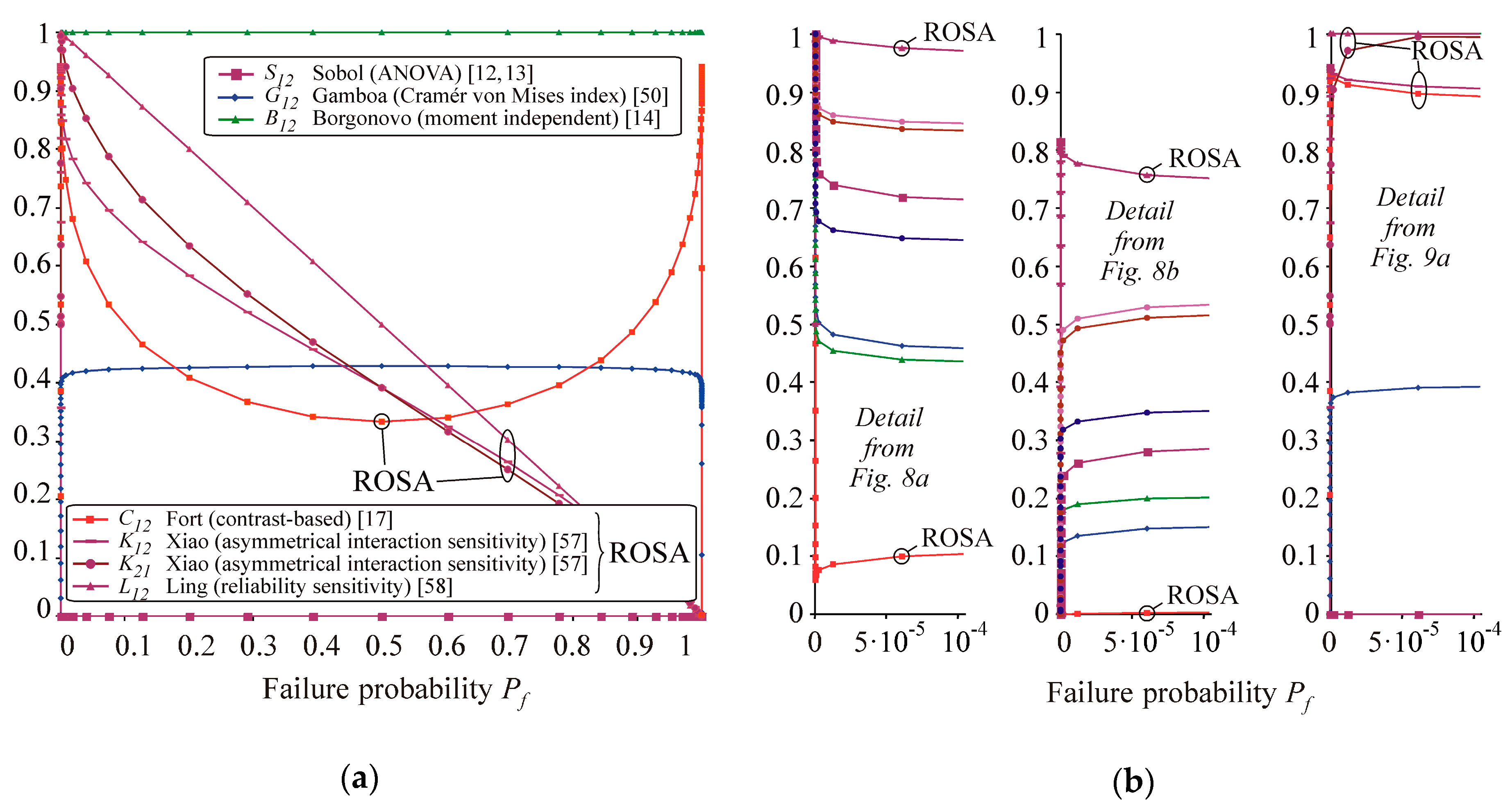
The first-order indices are depicted in Figure 8 and the second-order indices are depicted on the left part of Figure 9. Correlation coefficients corr(X1, Z) and corr(X2, Z) are added to Figure 8. Only indices within the interval [0, 1] are depicted. Omission sensitivity indices are not plotted because they have a value greater than one. The curves meet the expectation that small Pf (due to small μF and small σF) are less sensitive to F and more sensitive to R.
The parametric change of Pf (μF) influences the values of all indices. All first-order indices of variable X1 (R) are axially symmetrical to indices X2 (F) along the vertical axis Pf = 0.5 with the exception of Ling and Xiao indices. Xiao asymmetrical interaction indices are K12 ≠ K21 with the exception of Pf = 0.5 where K12 = K21. The plots of Borgonovo and Cramér–von Mises first-order indices are similar; the second-order indices are B12 = 1.0 and G12 = 1.0 − G1 − G12. The plots of Kendall’s tau coefficient and plots of Sobol’s indices are similar. The plots of Spearman’s and Pearson coefficients are also similar. On the left side of the graphs, contrast Pf indices reach their extreme at point Pf = 3.216·10−10, C1 = 0.06, C12 = 0.94, but no extreme on C2. On the right side of the graphs, the extreme is at point Pf = 1 − 3.216·10−10, C2 = 0.06, C12 = 0.94, but no extreme on C1. Ling and Xiao indices have an extreme at Pf = 3.216·10−10, K2 = L2 = 0.82, K12 = 0.94; other extremes of Ling and Xiao indices are difficult to identify numerically (compared to other indices) because they quickly attain relatively small or large values for large or small Pf.
For standard design case Pf = 7.2·10−5 we obtain K1 = L1 = 0.97, K2 = L2 = 0.76, K12 = 0.91, K12 = 0.994, L12 = 0.99993. A detail of the plot of sensitivity indices for Pf < 1·10−4 is depicted on the right part of Figure 9. For instance, for Pf = 7.2·10−5, we obtain O1 = 1.88, O2 = 1.18, or for Pf = 8.5·10−6, we obtain O1 = 1.99, O2 = 1.16.
5. Observation, Discussion and Questions
Reliability-oriented sensitivity indices (Xiao, Ling, Contrast and Madsen’s) are computed together with the global indices (Sobol, Borgonovo and Cramér–von Mises). The effects of R and F on structural reliability are first analysed separately for each of the eight selected sensitivity indices.
Contrast Pf indices have relatively small values of first-order indices and high values of second-order indices for small Pf. The numerical results of reliability engineering tasks [54,55] with five input random variables have shown that the smaller Pf is, the smaller the values of first-order indices and the higher the values of higher-order indices. Change in the mean value or standard deviation of the dominant variables had a clear effect on Pf, confirming the rationality of the contrast indices applied in [54]. The sum of all indices is equal to one, which makes it easier to compare SA results for different Pf associated with different reliabilities, for e.g., different design conditions, different stages of the structural life or different loading conditions. For very small values of Pf, Equation (29) can be written approximately as:
and similarly
The clear addressability to Pf is evident from Equation (30) and Equation (31). If the binary random variable 1Z<0 is considered, Equation (30) can then be written as:
where corr is Pearson correlation coefficient. SA based on contrast functions yields the same (symmetrical) results for unreliability (Pf) and reliability (1 − Pf) because Ci in Equation (29) is computed from the values of the contrast functions Pf (1 − Pf) and (Pf|Xi)(1 − (Pf|Xi)). If 1Z<0 is rare, the evaluation of Equation (32) using Monte Carlo type methods requires an extreme number of samples.
The sum of all Ling or Xiao indices is not equal to one. For small Pf, the values of the first-order indices are relatively high; moreover, the second-order index is always greater than the first-order index, which complicates the comparison of the influence on Pf. The advantage of computing Ling indices is that the computation of the higher-order indices does not depend on the computation (accuracy) of lower-order indices; therefore, their computation may be performed parallelly on multiple processor cores.
Cramér–von Mises indices have the sum of all indices equal to one. However, there is no addressability of indices to the Pf level because Equations (13) and (14) are integrated over all dΦZ(t), i.e., over all t (which means over all Pf). This is also the reason that, at intervals relevant to reliability, index values are not extremely high or low. The advantage is that a zero value of the Cramér-von Mises index clearly means that the input is not important. Triple-nested-loop computation makes these indices very numerically challenging. Nevertheless, numerous effective approaches to reduce this computational complexity already exist; see, for e.g., [61].
Borgonovo first-order indices yield reasonable values in intervals relevant to reliability, similar to Cramér–von Mises indices. The advantage of these indices is the transparency and the clear interpretation of the influence of input uncertainty on the entire output distribution regardless of the specific moment of the output (moment independence). Moreover, the indices can be computed even in the presence of correlation between input variables. The computational complexity of indices is not high. The disadvantage is that the sum of all indices is not equal to one and the indices are not directly addressable to Pf.
Sobol’s indices are functions of only the variance, which, although important, is not enough for SA of reliability. The computation of Sobol’s indices is based on the double-nested-loop computation and can be numerically very challenging for engineering tasks. However, if we consider the binary random variable 1Z<0 as the quantity of interest, Sobol’s indices can be an interesting reliability-oriented sensitivity technique [62].
Madsen’s factor can be applied as a computationally undemanding (simple) SA in engineering tasks, but with a number of limitations. Madsen’s factor can only be applied for Pf < 0.5. The disadvantage of Madsen’s factor is that factor Oi can have values significantly greater than 1. For example, in Case study 2, for Pf = 6.14·10−32 we obtain O1 = 32. A model with one random variable would theoretically lead to O1 = ∞. A significant computational problem can occur in non-linear problems when fixing to the mean value Xi leads to the limit case of a given physical phenomenon. For example, the amplitude of the axial curvature of a slender bar subjected to buckling has a mean value equal to zero, which means a perfectly straight bar [63]. The resistance of such a perfectly straight (unrealistic) bar is always higher than the resistance of a bar with any non-zero imperfection [64], and thus the mean value of zero is not suitable for fixing in reliability analysis or SA. The modification of Equation (27) to the form E(β|Xi)/β can be discussed, but with the proviso that fixing Xi must not lead to negative values of β. So far there is no global SA based on β, and it is questionable whether the first two statistical moments are sufficient to describe the influence on reliability.
The correlation coefficients are not directly addressable to Pf but can be used as sensitivity indicators if the output (Z) is monotonically dependent on the input variables R and F. Correlation points to dependence, but the opposite is not true. The advantage of correlation coefficients is their availability in computer software and they are relatively computationally inexpensive in simulation approaches.
ROSA-type indices have a different explanatory power than those of other types. Similar results cannot be expected from these two types (ROSA vs. non-ROSA) of indices as an input variable could be influential on Pf but not on the distribution of Z and conversely. Nevertheless, there is relatively good agreement between contrast Cramér–von Mises indices, Borgonovo indices and Pf indices in the interval of approximately Pf (0.1, 0.9). However, common building structures are designed with a reliability of Pf < 4.8·10−4; see Table 1. For such small Pf, only Cramér–von Mises indices and Borgonovo indices have similar values. The values of the other sensitivity indices are considerably different.
It can be concluded from all the obtained numerical results that if σF < σR (σF > σR), the sensitivity of Pf to R is higher (lower) than the sensitivity of Pf to F. It was confirmed that only ROSA-type indices are suitable for probability-based reliability assessment. The results of Case study 1 showed that change in μF together with σF = const. changes only the values of contrast Pf indices and Ling and Xiao indices, the other indices remain unchanged. Furthermore, change in σF together with μF = const. changes the values of all indices, except of course B12 = 1 and S12 = 0. The results of Case study 2 showed that changes in σF and μF with the condition vF = σF/μF = const. causes changes in the values of all indices; therefore, none of these indices is a pure indicator of the influence of vF on Pf.
It can be noted that resistance is generally a random variable that is a product of random variables such as yield strength (material characteristic), cross-sectional area (geometric characteristic), etc. Material and geometric characteristics usually do not have perfect Gauss pdf due to small skewness and kurtosis observed in histograms from real experiments [65,66]. The dead load can be roughly approximated using Gauss pdf, but other load types (wind, snow, traffic, long-term load action) have pdfs significantly different from Gauss pdf. For more complex structures, numerous load conditions and tens to hundreds of random variables with different pdfs can be expected. Furthermore, input random variables may have mutual correlations, which are implemented in beams [67] in more detail than in systems where each beam is represented by a smaller number of random variables independent of another beam; see for e.g., [68].
The question is, to what extent can different types of sensitivity indices oriented to Pf be influenced by the skewness and kurtosis values of the input variables or by correlations between them, and what is its importance for the analysis of reliability? For instance, the values of Sobol’s indices change when the kurtosis changes, but not when the skewness changes [34]. Of the SA types presented here, only Borgonovo indices [14] have the ability to have correlations between input variables. This ability must also be sought in other indices suitable for structural reliability analysis.
A generally accepted measure of reliability is Pf; therefore, Pf should be the overall objective of SA. However, the concept of Eurocodes [19] assesses reliability according to the limit states using the so-called semi-probabilistic method, which compares the design values (quantiles) of resistance and load. Because probabilistic reliability analysis would be too expensive in common engineering practice, design values are usually computed deterministically according to design standards. These design values can be verified using the lower quantity of resistance (for e.g., 0.1 percentile) and upper quantity of load, where resistance and load are functions of other random variables; see Figure 2. Another useful property of SA could be that sensitivity indices oriented to Pf and design quantiles form pairs based on the same theoretical basis. For example, global SA subordinated to contrasts can be associated with both Pf and quantities Rd and Fd; see Figure 2. However, the question is whether there is a link between indices Equations (17), (18) and (20), (21) when the contrast functions Equations (16) and (19) are different. Preliminary studies show that partial similarity can be expected between the total indices.
6. Conclusions
The presented case studies have shown that the numerical results of reliability-oriented sensitivity analysis (ROSA) are inconsistent. ROSA was evaluated using Contrast, Xiao, Ling and Madsen’s indices. For structural reliability, the key quantity of interest is failure probability Pf, which is lower than 4.8·10−4.
Contrast Pf indices have relatively small values of first-order indices and high values of second-order indices for small Pf. Ling or Xiao indices have relatively high values of first-order indices, but also high values of second-order indices for small Pf. For instance, in the first case study, if Pf → 0 then C1 = 0, C2 = 0, C12 = 1 and L1 = 1, L2 = 1, L12 = 1. In civil engineering, Pf is generally very small, and extreme values of sensitivity indices estimated by ROSA can be expected. The advantage of contrast Pf indices is that the sum of all indices is equal to one. The sum of all Ling or Xiao indices is not equal to one. The Madsen factor values were significantly greater than 1 and therefore cannot be compared in size with Contrast, Xiao and Ling indices. Madsen’s factor does not reflect change in the mean value of input variables, although this change causes a change in Pf.
In contrast, Xiao, Ling and Madsen’s indices have correctly identified the order of importance of input random variables to Pf; however, this observation only applies to the presented case studies and cannot be generalized. In the case studies, it is not possible to determine, even approximately, the percentage by which the dominant variable is more influential than the others, so this conclusion is true for each type of SA. Structural reliability lacks a common platform of SA that provides a clear interpretation of the size of sensitivity indices and defines their information value.
The other indices (Sobol, Borgonovo and Cramér–von Mises) and correlation coefficients are not directly addressable to Pf and therefore are not generally suitable for the analysis of reliability. As expected, these (out of ROSA type) sensitivity indices do not reflect the change in mean value of input variables, although this change causes a change in Pf. This means that the two variables that have a different influence on the reliability may have the same indices. In relation to the reliability of structures, the information value of these indices is not unambiguous. In the case of ROSA, Xiao and Ling indices, no two different Pf values exist for which the same sets of sensitivity indices exist, but contrast Pf indices have the same or similar values for unreliability (Pf) and reliability (1 − Pf).
There are many engineering reliability assessments in which non-ROSA indices are applied, although the connection with reliability is mentioned. The reason for these applications may be the simplicity of evaluating indices as well as the experience that known indices have at least partial sensitivity for reliability, which, along with other experience, is sufficient for basic decision-making. With the development of ROSA, a gradual transition to new types of reliability-oriented indices can be expected.
In connection with sustainable reliability, it is possible to discuss which type of ROSA should be applied and which key quantities of interest ROSA should be oriented to in particular. The Eurocode standards for structural design assess reliability using a so-called semi-probabilistic approach, which is based on design quantiles. The question remains whether Pf can be adequately replaced by design quantities, reliability index β or other model-based inferences so that the information value of SA results in relation to reliability is approximately maintained. Design quantiles are an important part of reliability analysis, and SA of the design quantiles may be required to provide results consistent with Pf.
In general, ROSA directly addressable to Pf may be preferred rather than focusing on the reliability index β or quantiles. Indices with the sum of one and a clear addressability to Pf present one SA, an advantage that facilitates the comparison of the results of different probability models. Contrast functions are a more general tool for estimating various parameters associated with probability distributions, and thus the partial consistency of requirements could perhaps be sought on the basis of contrasts. These and other tasks need to be addressed in order to make SA of structural reliability a useful and practical tool.
Funding
The work has been supported and prepared within the project namely “Probability oriented global sensitivity measures of structural reliability“ of The Czech Science Foundation (GACR, https://gacr.cz/) no. 20-01734S, Czechia.
Conflicts of Interest
The author declares no conflict of interest.
References
- Benjamin, J.R.; Cornell, C.A. Probability, Statistics, and Decision for Civil Engineers; McGraw-Hill: New York, NY, USA, 1970. [Google Scholar]
- Au, S.-K.; Wang, Y. Engineering Risk Assessment with Subset Simulation; Wiley: New York, NY, USA, 2014. [Google Scholar]
- Chabridon, V. Reliability-Oriented Sensitivity Analysis under Probabilistic Model Uncertainty—Application to Aerospace Systems. Ph.D. Thesis, University Clermont Auvergne, Clermont-Ferrand, France, 2018. [Google Scholar]
- Melchers, R.E.; Ahammed, M. A fast-approximate method for parameter sensitivity estimation in Monte Carlo structural reliability. Comput. Struct. 2004, 82, 55–61. [Google Scholar] [CrossRef]
- Wang, P.; Lu, Z.; Tang, Z. A derivative based sensitivity measure of failure probability in the presence of epistemic and aleatory uncertainties. Comput. Math. Appl. 2013, 65, 89–101. [Google Scholar] [CrossRef]
- Jensen, H.A.; Mayorga, F.; Papadimitriou, C. Reliability sensitivity analysis of stochastic finite element models. Comput. Methods. Appl. Mech. Eng. 2015, 296, 327–351. [Google Scholar] [CrossRef] [Green Version]
- MiarNaeimi, F.; Azizyan, G.; Rashki, M. Reliability sensitivity analysis method based on subset simulation hybrid techniques. Appl. Math. Model. 2019, 75, 607–626. [Google Scholar] [CrossRef]
- Kala, Z.; Valeš, J. Sensitivity assessment and lateral-torsional buckling design of I-beams using solid finite elements. J. Constr. Steel. Res. 2017, 139, 110–122. [Google Scholar] [CrossRef]
- Saltelli, A.; Ratto, M.; Andres, T.; Campolongo, F.; Cariboni, J.; Gatelli, D.; Saisana, M.; Tarantola, S. Global Sensitivity Analysis: The Primer; John Wiley & Sons: West Sussex, UK, 2008. [Google Scholar]
- Saltelli, A.; Marivoet, J. Non-parametric statistics in sensitivity analysis for model output: A comparison of selected techniques. Reliab. Eng. Syst. Saf. 1990, 28, 229–253. [Google Scholar] [CrossRef]
- Xiao, S.; Lu, Z.; Xu, L. A new effective screening design for structural sensitivity analysis of failure probability with the epistemic uncertainty. Reliab. Eng. Syst. Saf. 2016, 156, 1–14. [Google Scholar] [CrossRef]
- Sobol, I.M. Sensitivity estimates for non-linear mathematical models. Math. Model. Comput. Exp. 1993, 1, 407–414. [Google Scholar]
- Sobol, I.M. Global sensitivity indices for nonlinear mathematical models and their Monte Carlo estimates. Math. Comput. Simul. 2001, 55, 271–280. [Google Scholar] [CrossRef]
- Borgonovo, E. A new uncertainty importance measure. Reliab. Eng. Syst. Saf. 2007, 92, 771–784. [Google Scholar] [CrossRef]
- Borgonovo, E.; Castaings, W.; Tarantola, S. Moment independent importance measures: New results and analytical test cases. Risk Anal. 2011, 31, 404–428. [Google Scholar] [CrossRef] [PubMed]
- Borgonovo, E. Measuring uncertainty importance: Investigation and comparison of alternative approaches. Risk Anal. 2006, 26, 1349–1361. [Google Scholar] [CrossRef] [PubMed]
- Fort, J.C.; Klein, T.; Rachdi, N. New sensitivity analysis subordinated to a contrast. Commun. Stat. Theory Methods 2016, 45, 4349–4364. [Google Scholar] [CrossRef] [Green Version]
- Wang, Y.; Xiao, S.; Lu, Z. An efficient method based on Bayes’ theorem to estimate thefailure-probability-based sensitivity measure. Mech. Syst. Signal. Process. 2019, 115, 607–620. [Google Scholar] [CrossRef]
- European Committee for Standardization. EN 1990:2002: Eurocode—Basis of Structural Design; European Committee for Standardization: Brussels, Belgium, 2002. [Google Scholar]
- Borgonovo, E.; Hazen, G.; Plischke, E. A Common rationale for global sensitivity measures and their estimation. Comput. Struct. 2016, 36, 1871–1895. [Google Scholar] [CrossRef]
- Greegar, G.; Manohar, G.S. Global response sensitivity analysis using probability distance measures and generalization of Sobol’s analysis. Probabilistic Eng. Mech. 2015, 41, 21–33. [Google Scholar] [CrossRef]
- Kotełko, M.; Lis, P.; Macdonald, M. Load capacity probabilistic sensitivity analysis of thin-walled beams. Thin Walled Struct. 2017, 115, 142–153. [Google Scholar] [CrossRef] [Green Version]
- Štefaňák, J.; Kala, Z.; Miča, L.; Norkus, A. Global sensitivity analysis for transformation of Hoek-Brown failure criterion for rock mass. J. Civ. Eng. Manag. 2018, 24, 390–398. [Google Scholar] [CrossRef]
- Mahmoudi, E.; Hölter, R.; Georgieva, R.; König, M.; Schanz, T. On the global sensitivity analysis methods in geotechnical engineering: A comparative study on a rock salt energy storage. Int. J. Civ. Eng. 2019, 17, 131–143. [Google Scholar] [CrossRef]
- Tate, E.; Munoz, C.; Suchan, J. Uncertainty and sensitivity analysis of the HAZUS-MH flood model. Nat. Hazards Rev. 2014, 16, 04014030. [Google Scholar] [CrossRef]
- Pang, Z.; O’Neill, Z.; Li, Y.; Niu, F. The role of sensitivity analysis in the building performance analysis: A critical review. Energy Build. 2020, 209, 109659. [Google Scholar] [CrossRef]
- Su, L.; Wang, T.; Li, H.; Cao, Y.; Wang, L. Multi-criteria decision making for identification of unbalanced bidding. J. Civ. Eng. Manag. 2020, 26, 43–52. [Google Scholar] [CrossRef]
- Salimi, S.; Hammad, A. Sensitivity analysis of probabilistic occupancy prediction model using big data. Build. Environ. 2020, 172, 106729. [Google Scholar] [CrossRef]
- Saltelli, A.; Benini, L.; Funtowicz, S.; Giampietro, M.; Kaiser, M.; Reinert, E.; Van der Sluijs, J.P. The technique is never neutral. How methodological choices condition the generation of narratives for sustainability. Environ. Sci. Policy 2020, 106, 87–98. [Google Scholar] [CrossRef]
- Ferretti, F.; Saltelli, A.; Tarantola, S. Trends in sensitivity analysis practice in the last decade. Sci. Total Environ. 2016, 568, 666–670. [Google Scholar] [CrossRef] [PubMed]
- Joint Committee on Structural Safety (JCSS). Probabilistic Model Code. Available online: https://www.jcss-lc.org/ (accessed on 15 May 2020).
- Sedlacek, G.; Kraus, O. Use of safety factors for the design of steel structures according to the Eurocodes. Eng. Fail. Anal. 2007, 14, 434–441. [Google Scholar] [CrossRef]
- Kala, Z. Geometrically non-linear finite element reliability analysis of steel plane frames with initial imperfections. J. Civ. Eng. Manag. 2012, 18, 81–90. [Google Scholar] [CrossRef]
- Kala, Z.; Valeš, J. Global sensitivity analysis of lateral-torsional buckling resistance based on finite element simulations. Eng. Struct. 2017, 134, 37–47. [Google Scholar] [CrossRef]
- Szymczak, C. Sensitivity analysis of thin-walled members, problems and applications. Thin Walled Struct. 2003, 41, 271–290. [Google Scholar] [CrossRef]
- Mang, H.A.; Höfinger, G.; Jia, X. On the interdependency of primary and initial secondary equilibrium paths in sensitivity analysis of elastic structures. Comput. Methods Appl. Mech. Eng. 2011, 200, 1558–1567. [Google Scholar] [CrossRef]
- Hassan, M.S.; Salawdeh, S.; Goggins, J. Determination of geometrical imperfection models in finite element analysis of structural steel hollow sections under cyclic axial loading. J. Constr. Steel Res. 2018, 141, 189–203. [Google Scholar] [CrossRef]
- Wu, J.; Zhu, J.; Dong, Y.; Zhang, Q. Nonlinear stability analysis of steel cooling towers considering imperfection sensitivity. Thin Walled Struct. 2020, 146, 106448. [Google Scholar] [CrossRef]
- Rykov, V.; Zaripova, E.; Ivanova, N.; Shorgin, S. On sensitivity analysis of steady state probabilities of double redundant renewable system with Marshall-Olkin failure model. Commun. Comput. Inf. Sci. 2018, 919, 234–245. [Google Scholar]
- Jönsson, J.; Müller, M.S.; Gamst, C.; Valeš, J.; Kala, Z. Investigation of European flexural and lateral torsional buckling interaction. J. Constr. Steel Res. 2019, 156, 105–121. [Google Scholar] [CrossRef]
- Antucheviciene, J.; Kala, Z.; Marzouk, M.; Vaidogas, E.R. Solving civil engineering problems by means of fuzzy and stochastic MCDM methods: Current state and future research. Math. Probl. Eng. 2015, 2015, 362579. [Google Scholar] [CrossRef] [Green Version]
- Zavadskas, E.K.; Antucheviciene, J.; Vilutiene, T.; Adeli, H. Sustainable decision-making in civil engineering, construction and building technology. Sustainability 2018, 10, 14. [Google Scholar] [CrossRef] [Green Version]
- Lehký, D.; Pan, L.; Novák, D.; Cao, M.; Šomodíková, M.; Slowik, O. A comparison of sensitivity analyses for selected prestressed concrete structures. Struct. Concr. 2019, 20, 38–51. [Google Scholar] [CrossRef] [Green Version]
- Novák, L.; Novák, D. On the possibility of utilizing Wiener-Hermite polynomial chaos expansion for global sensitivity analysis based on Cramér-von Mises distance. In Proceedings of the 2019 International Conference on Quality, Reliability, Risk, Maintenance, and Safety Engineering, QR2MSE 2019, Zhangjiajie, China, 6–9 August 2019; pp. 646–654. [Google Scholar]
- Wen, Z.; Xia, Y.; Ji, Y.; Liu, Y.; Xiong, Z.; Lu, H. Study on risk control of water inrush in tunnel construction period considering uncertainty. J. Civ. Eng. Manag. 2019, 25, 757–772. [Google Scholar] [CrossRef] [Green Version]
- Karasan, A.; Zavadskas, E.K.; Kahraman, C.; Keshavarz-Ghorabaee, M. Residential construction site selection through interval-valued hesitant fuzzy CODAS method. Informatica 2019, 30, 689–710. [Google Scholar] [CrossRef]
- Zhao, Y.G.; Ono, T. A general procedure for first/second-order reliability method (FORM/SORM). Struct. Saf. 1999, 21, 95–112. [Google Scholar] [CrossRef]
- Kala, Z. Reliability analysis of the lateral torsional buckling resistance and the ultimate limit state of steel beams with random imperfections. J. Civ. Eng. Manag. 2015, 21, 902–911. [Google Scholar] [CrossRef]
- Sedlacek, G.; Müller, C. The European standard family and its basis. J. Constr. Steel Res. 2006, 62, 522–548. [Google Scholar] [CrossRef]
- Gamboa, F.; Klein, T.; Lagnoux, A. Sensitivity analysis based on Cramér-von Mises distance. SIAM ASA J. Uncertain. Quantif. 2018, 6, 522–548. [Google Scholar] [CrossRef] [Green Version]
- Plischke, E.; Borgonovo, E. Copula theory and probabilistic sensitivity analysis: Is there a connection? Eur. J. Oper. Res. 2019, 277, 1046–1059. [Google Scholar] [CrossRef]
- McKey, M.D.; Beckman, R.J.; Conover, W.J. Comparison of the three methods for selecting values of input variables in the analysis of output from a computer code. Technometrics 1979, 21, 239–245. [Google Scholar]
- Iman, R.C.; Conover, W.J. Small sample sensitivity analysis techniques for computer models with an application to risk assessment. Commun. Stat. Theory Methods 1980, 9, 1749–1842. [Google Scholar] [CrossRef]
- Kala, Z. Global sensitivity analysis of reliability of structural bridge system. Eng. Struct. 2019, 194, 36–45. [Google Scholar] [CrossRef]
- Kala, Z. Estimating probability of fatigue failure of steel structures. Acta Comment. Univ. Tartu. Math. 2019, 23, 245–254. [Google Scholar] [CrossRef]
- Kala, Z. Quantile-oriented global sensitivity analysis of design resistance. J. Civ. Eng. Manag. 2019, 25, 297–305. [Google Scholar] [CrossRef] [Green Version]
- Xiao, S.; Lu, Z. Structural reliability sensitivity analysis based on classification of model output. Aerosp. Sci. Technol. 2017, 71, 52–61. [Google Scholar] [CrossRef]
- Ling, C.; Lu, Z.; Cheng, K.; Sun, B. An efficient method for estimating global reliability sensitivity indices. Probabilistic Eng. Mech. 2019, 56, 35–49. [Google Scholar] [CrossRef]
- Madsen, H.O. Omission sensitivity factor. Struct. Saf. 1988, 5, 35–45. [Google Scholar] [CrossRef]
- Leander, J.; Al-Emrani, M. Reliability-based fatigue assessment of steel bridges using LEFM—A sensitivity analysis. Int. J. Fatigue 2016, 93, 82–91. [Google Scholar] [CrossRef]
- Sudret, B. Global sensitivity analysis using polynomial chaos expansions. Reliab. Eng. Syst. Saf. 2008, 93, 964–979. [Google Scholar] [CrossRef]
- Wei, P.; Lu, Z.; Hao, W.; Feng, J.; Wang, B. Efficient sampling methods for global reliability sensitivity analysis. Comput. Phys. Commun. 2012, 183, 1728–1743. [Google Scholar] [CrossRef]
- Kala, Z. Sensitivity assessment of steel members under compression. Eng. Struct. 2009, 31, 1344–1348. [Google Scholar] [CrossRef]
- Mercier, C.; Khelil, A.; Khamisi, A.; Al Mahmoud, F.; Boissiere, R.; Pamies, A. Analysis of the global and local imperfection of structural members and frames. J. Civ. Eng. Manag. 2019, 25, 805–818. [Google Scholar] [CrossRef]
- Melcher, J.; Kala, Z.; Holický, M.; Fajkus, M.; Rozlívka, L. Design characteristics of structural steels based on statistical analysis of metallurgical products. J. Constr. Steel Res. 2004, 60, 795–808. [Google Scholar] [CrossRef]
- Kala, Z.; Melcher, J.; Puklický, L. Material and geometrical characteristics of structural steels based on statistical analysis of metallurgical products. J. Civ. Eng. Manag. 2009, 15, 299–307. [Google Scholar] [CrossRef]
- Kala, Z.; Valeš, J.; Jönsson, L. Random fields of initial out of straightness leading to column buckling. J. Civ. Eng. Manag. 2017, 23, 902–913. [Google Scholar] [CrossRef] [Green Version]
- Kala, Z. Sensitivity analysis of steel plane frames with initial imperfections. Eng. Struct. 2011, 33, 2342–2349. [Google Scholar] [CrossRef]
Figure 1.
Illustration of the reliability index β.

Figure 2.
Illustration of the design condition of reliability.

Figure 3.
Static model: (a) bar under axial tension; (b) probability density functions of R and F.

Figure 4.
Case study 1, probability density functions of R and F.

Figure 5.
Case study 1, first-order sensitivity indices of (a) resistance R; (b) load Action F.

Figure 6.
Case study 1: (a) second-order sensitivity indices of R, F; (b) sensitivity analysis (SA) results related to structural reliability.
Figure 6.
Case study 1: (a) second-order sensitivity indices of R, F; (b) sensitivity analysis (SA) results related to structural reliability.

Figure 7.
Case study 2, probability density functions of R and F.

Figure 8.
Case study 2, first-order sensitivity indices of (a) Resistance R; (b) Load Action F.

Figure 9.
Case study 2: (a) Second-order sensitivity indices of R, F; (b) SA results related to structural reliability.
Figure 9.
Case study 2: (a) Second-order sensitivity indices of R, F; (b) SA results related to structural reliability.


Table 1.
Recommended minimum values of β and related Pf.
| Reliability Class | β | Pf |
|---|---|---|
| RC3 | 4.3 | 8.5·10−6 |
| RC2 | 3.8 | 7.2·10−5 |
| RC1 | 3.3 | 4.8·10−4 |
© 2020 by the author. Licensee MDPI, Basel, Switzerland. This article is an open access article distributed under the terms and conditions of the Creative Commons Attribution (CC BY) license (http://creativecommons.org/licenses/by/4.0/).
Share and Cite
MDPI and ACS Style
Kala, Z. Sensitivity Analysis in Probabilistic Structural Design: A Comparison of Selected Techniques. Sustainability 2020, 12, 4788. https://0-doi-org.brum.beds.ac.uk/10.3390/su12114788
AMA Style
Kala Z. Sensitivity Analysis in Probabilistic Structural Design: A Comparison of Selected Techniques. Sustainability. 2020; 12(11):4788. https://0-doi-org.brum.beds.ac.uk/10.3390/su12114788
Chicago/Turabian StyleKala, Zdeněk. 2020. "Sensitivity Analysis in Probabilistic Structural Design: A Comparison of Selected Techniques" Sustainability 12, no. 11: 4788. https://0-doi-org.brum.beds.ac.uk/10.3390/su12114788
Note that from the first issue of 2016, this journal uses article numbers instead of page numbers. See further details here.