Sentiment Digitization Modeling for Recommendation System

Abstract

As the importance of providing personalized services increases, various studies on personalized recommendation systems are actively being conducted. Among the many methods used for recommendation systems, the most widely used is collaborative filtering. However, this method has lower accuracy because recommendations are limited to using quantitative information, such as user ratings or amount of use. To address this issue, many studies have been conducted to improve the accuracy of the recommendation system by using other types of information, in addition to quantitative information. Although conducting sentiment analysis using reviews is popular, previous studies show the limitation that results of sentiment analysis cannot be directly reflected in recommendation systems. Therefore, this study aims to quantify the sentiments presented in the reviews and reflect the results to the ratings; that is, this study proposes a new algorithm that quantifies the sentiments of user-written reviews and converts them into quantitative information, which can be directly reflected in recommendation systems. To achieve this, the user reviews, which are qualitative information, must first be quantified. Thus, in this study, sentiment scores are calculated through sentiment analysis by using a text mining technique. The data used herein are from movie reviews. A domain-specific sentiment dictionary was constructed, and then based on the dictionary, sentiment scores of the reviews were calculated. The collaborative filtering of this study, which reflected the sentiment scores of user reviews, was verified to demonstrate its higher accuracy than the collaborative filtering using the traditional method, which reflects only user rating data. To overcome the limitations of the previous studies that examined the sentiments of users based only on user rating data, the method proposed in this study successfully enhanced the accuracy of the recommendation system by precisely reflecting user opinions through quantified user reviews. Based on the findings of this study, the recommendation system accuracy is expected to improve further if additional analysis can be performed.

1. Introduction

It is estimated that more than 2.5 trillion MB of data are generated per day worldwide, at the current pace, and the pace of this generation is increasing by 60% each year. Online accessibility has made it possible to store large amounts of data while mitigating the physical limitation of offline storage. However, with the increase in the amount of accessible information, more people are feeling extreme exhaustion from the flood of newly generated information every day. As reviewing every piece of information is merely impossible, there are many difficulties in finding and selecting information that suits the preferences of each user. Thus, the necessity of a recommendation system that can remove unnecessary information from a large of number data and provide information according to individual preferences is gradually increasing.

Previous studies on recommendation systems that provided personalized information to users were generally focused on analyses using structured data, which are easy to quantify, such as user purchase history, product ratings, and number of visits [1]. Among the data, rating data have been used in the recommendation systems as the most popular index of user preference. However, in recent years, recommendations limited to using only the user rating data as the index to indicate user preferences provided low accuracy [2,3]. This indicates that there were limitations in recommendation system developments as the detailed and elaborate preferences of users are not reflected. Although the same rating scores of 10 points may be given by a user to two different movies, the intensity of the sentiments found in the user review texts may be different for these movies. Despite the same quantitative rating scores, this could be the crucial factor that reduces the accuracy of the recommendation system.

Owing to its high usability and its effortless processing of explicit information into a mathematical system, collaborative filtering using user ratings has been widely used. However, questions have been raised whether the user rating information properly reflects the user preferences. This uncertainty has led to various studies that developed collaborative filtering models that better reflect user preferences [4].

Many researchers have focused on text reviews in making rating predictions. The text reviews serve as a useful tool in the recommendation systems as they provide detailed preferences of what the user might have for a specific item. Various studies have also confirmed that the user text reviews play an important role in developing a recommendation system [5,6].

Since human-centered urban services should identify what people need, address their various needs, and set a vision by reinterpreting the city, various fields should be involved, such as culture, architecture, city, civil engineering, transportation, and machinery. As a city without people has no meaning, it is natural for the environment to change centered on human beings. In order to develop a new city, we should pay attention to each person who belongs to it, not the physical environment. Furthermore, if there is a request from a single individual, no matter how trivial it is, a series of efforts are required to actively respond to the request.

In order to analyze and utilize such request, making the most of big data is important more than anything else. Big data analysis is a method of analyzing a huge amount of data arising from the use of wired/wireless Internet and social network services (SNS), and various studies on this have been actively underway.

In particular, data on movies are a typical data that help to verify human emotion indicators and can be applied to personalized urban services. Accordingly, research on recommendation systems through movie analysis using big data has been steadily increasing. The public’s preferences for products and movies are analyzed by classifying emotions that appear in product reviews, product use reviews, and movie reviews written by unspecified individuals as negative or positive. By combining the analyzed preferences with personalized information, it is used in various recommendation system areas appropriate for the user propensity.

In this study, to improve the accuracy of existing recommendation systems, which used only quantitative data, a model that precisely corrects ratings by quantifying the sentiments of user reviews, which are qualitative data, is proposed. In addition, an algorithm that improves the recommendation system accuracy is proposed by applying review sentiment scores to the ratings. This study constructs a domain-specific dictionary based on the reviews, which are qualitative data generated by users. Then, using the dictionary, an algorithm that can improve the accuracy of the recommendation system is derived by extracting the sentiment scores of the texts and reflecting them to the ratings (i.e., quantitative data).

2. Related Research

2.1. Recommendation System

The aim of the recommendation system is to provide suggestions to users with items that fit the user preference criteria, based on various factors, such as demographic information, purchase history, and expected interest of the user. Since the successful recommendation system implementations by Netflix and Amazon, various efforts have also been made in Korea to recommend users with items relevant to their preferences. Some examples of this include a movie recommendation system by WATCHA and top news recommendation through NAVER AiRS, and Kakao’s RUBICS, which recommends content by analyzing user responses in real time. Thus, recommendation systems are widely used in our daily lives, and studies related to these systems are continuously being conducted. A collaborative filtering method is used for the popular recommendation algorithm that is most frequently used [7].

Collaborative filtering is a preference predicting method that is based on similarities between users or items, using a basic assumption that the users with similar preferences on one particular item will show similar preferences on the other item [8]. The collaborative filtering method can be mainly classified into memory-based and model-based algorithms. The memory-based algorithm, also referred to as a neighborhood model, is an algorithm that predicts the rating that a user might give by constructing a user-item matrix of all users and by finding similar users or items based on the user or item information. This method is divided into user-based and item-based collaborative filtering [9].

The user-based collaborating filtering is a method of recommending items that are commonly desired by neighboring users, after defining neighboring users who have similar desires to the user, based on the rating information provided by the user.

The basic concept is shown in Figure 1. In the figure, the user with the most similar preferences to the recommendation target user is “User C,” who purchased “Item 1,” “Item 2,” and “Item 5.” Based on the information of “User C,” “Item 7,” which has been preferred by “User C” but not by the target user yet, is chosen and recommended to the target user.

Item-based collaborative filtering recommendation is used for YouTube and Netflix video recommendations and Amazon product recommendations [10].

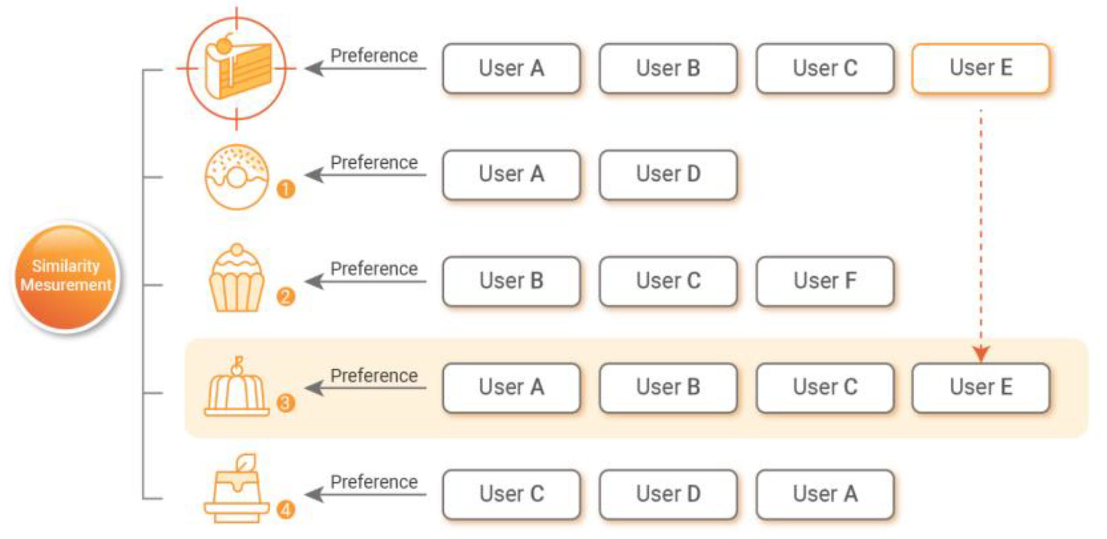
The basic concept is shown in Figure 2. The item with the highest similarity is chosen among the recommendation items. The selected “Item 3” is presented as the recommended item to “User E”, who has not yet purchased the recommended item.

The model-based algorithm employs the base process of a memory-based collaborating filtering method and uses machine learning or data mining techniques in the clustering, classification, and prediction processes [11]. Matrix factorization and clustering models are techniques that predict ratings on the unrated items by modeling users based on past user ratings. The matrix factorization method is a rating prediction method that uses latent factors, instead of a direct relationship between a user and an item. The most widely used algorithms are the singular value decomposition (SVD) and SVD++ algorithms. The clustering model enables individuals with similar characteristics to be grouped together using similarity measures between individuals [12]. The most widely used algorithms include the k-means and DBSCAN algorithms.

2.2. Recommendation System Reflecting User Reviews

As an example related to the recommendation system reflecting user reviews, one study developed a model that estimates the trend and intensity of positive or negative sentiment found in user reviews. Based on this model, sentiment analysis was conducted using a collaborative filtering recommendation system to classify whether the user is an optimist or pessimist [13,14]. Moreover, collaborated filtering was carried out for each group to set the user reviews as a criterion for group classification. One study extracted words that have a high relevance to the ratings and conducted multi-category classification featuring a neutral category, in addition to positive and negative categories, based on the frequency of the extracted words [15]. Thus, many studies have been conducted to include the classification of multiple sentiments, such as neutral, in addition to classifying sentiments into only a positive and negative dichotomy. Further, various attempts have been consistently made to predict ratings by constructing sentiment dictionaries by creating a group of sentiment sentences related to opinions and assessments in reviews and then applying these sentences to movie reviews to infer ratings from 1 to 10, according to polarity [16]. However, these studies have the limitations of information loss as they do not directly reflect the review data in the algorithms. In recent studies related to sentiment analysis, sentiment scores have been investigated to measure the degree of sentiment rather than the classification. Hence, numerous studies that comprehend the degree of sentiment are also actively being conducted.

2.3. Recommendation System Using Sentiment Analysis

As social media and social network services (SNS) have become popular, the public has become the source of information as well as being the information consumer. The public generally expresses their feelings or opinions by posting comments and thoughts on various websites and SNS platforms. Consequently, with the increase in review data flow, interests in sentiment analysis also increased.

Sentiment analysis is a method that extracts subjective attitudes or sentiments of people based on text mining, which is one of the important areas of big data. Among previous studies and recommendation systems that use sentiment analysis, one study proposed a movie recommendation system by extracting emotion-related words from user reviews and comments to recommend personalized movies to individuals. In another study, the possibility of recommending appropriate movies to users was demonstrated through analysis of the sentiments of emotion-related words extracted from the sentiment lexicon, SentiWordNet [17]. Another study defined a review ontology, which is an emotion word dictionary for movies, to evaluate the sentiments of ratings and reviews [18]. Based on this, the study recommended customized movies to users by using a collaborated filtering method and context-based technique to analyze the sentiment level of emotion-related words of movie reviews. In addition, there is a study that used feedback given by restaurant customers to build a recommendation system based on user attributes and characteristics, by classifying positive and negative emotions and calculating sentiment scores through SentiWordNet [19]. In addition to the mentioned examples, there is also a study that showed a recommendation performance improvement by reflecting user review mining in the traditional recommendation algorithm, which was based on ratings [20].

Previous studies on recommendation systems using sentiment analysis mainly consist of using sentiment lexicons, such as SentiWordNet. Various studies on sentiment analysis in English have been actively conducted using lexicons such as AFFIN, SentiWordNet, and EmoLex. However, studies on sentiment analysis in the Korean language are relatively insufficient compared with English. This may be due to the linguistic characteristics of the Korean language. To conduct sentiment analysis, part-of-speech tagging should be performed first on nouns, verbs, and adjectives, in the process of natural language processing. In the case of English, part-of-speech tagging can be easily performed using the space between the words, as English is an inflected language with the tendency to have part-of-speech breaks with spaces. Contrary to this, the Korean language is an agglutinating language. Hence, there are many cases where the part-of-speech cannot be distinguished by spaces between words. Owing to this reason, studies on sentiment analysis using Korean texts have not been actively conducted.

2.4. Dictionary Construction-Based Sentiment Analysis

Dictionary-based sentiment analysis is the methodology of quantifying user reviews by matching the collected review data, which have been pre-processed, with a pre-constructed sentiment dictionary. Although the degree of sentiment is easy to understand when a dictionary is used, if the sentiment analysis is conducted using a general sentiment dictionary, the same words could have completely opposite sentiments in some cases, depending on the domain, which consequently could return a poor accuracy. Therefore, to correctly conduct sentiment analysis, specialized dictionaries using the domain characteristics for each application field should be constructed. Furthermore, because the same vocabulary can be used with different meanings, depending on the characteristics of the topic to be analyzed, constructing different sentiment dictionaries according to the characteristics of each domain is suggested for higher performance, rather than using a general sentiment dictionary [21].

To conduct sentiment analysis, numerous studies have been conducted on constructing appropriate sentiment dictionaries for given domains. One study improved the classification prediction accuracy by constructing a sentiment dictionary by extracting hospital-specific sentiment vocabulary and polarity values using 4300 “voice of customer” data, collected from a medical institution webpage. Another study constructed a sentiment dictionary specialized for the stock market domain from economic news data to improve the prediction accuracy of the stock market index [22]. In addition, one study verified that conducting sentiment analysis using a sentiment dictionary constructed for a specific topic significantly improves the prediction accuracy, compared to using a general sentiment dictionary [23].

The basic summary of the abovementioned previous studies is as follows: Typically, quantitative data, such as ratings, purchase history, and number of visits, have been utilized to conduct the most widely used collaborative filtering. In recent years, commonly used rating data have been found to be one of the major causes of the low accuracy of recommendation systems. Based on this finding, various methods have been proposed to improve the recommendation system accuracy. A popular method that uses user reviews in the recommendation system was proposed. However, it was limited to classifying the reviews only into positive, neutral, and negative sentiments and, thus, cannot reflect the detailed user satisfaction found in the reviews. As the number of studies on analyzing the degree of sentiment increased, studies that apply the results of these analyses to the recommendation systems have been actively conducted. However, in the case of Korean language, the number of publicly available sentiment dictionaries is very limited, and the existing dictionaries are only general dictionaries, instead of domain-specific dictionaries, hence limiting the recommendation accuracy.

3. Proposed Method

This study proposes a model that aims to improve the accuracy of the recommendation system by calculating review sentiment scores and integrating them with user ratings. In more detail, a domain-specific sentiment dictionary is constructed to derive the sentiment scores of user reviews. Then, based on the dictionary, the sentiment scores of the user review data are calculated and reflected in the recommendation system.

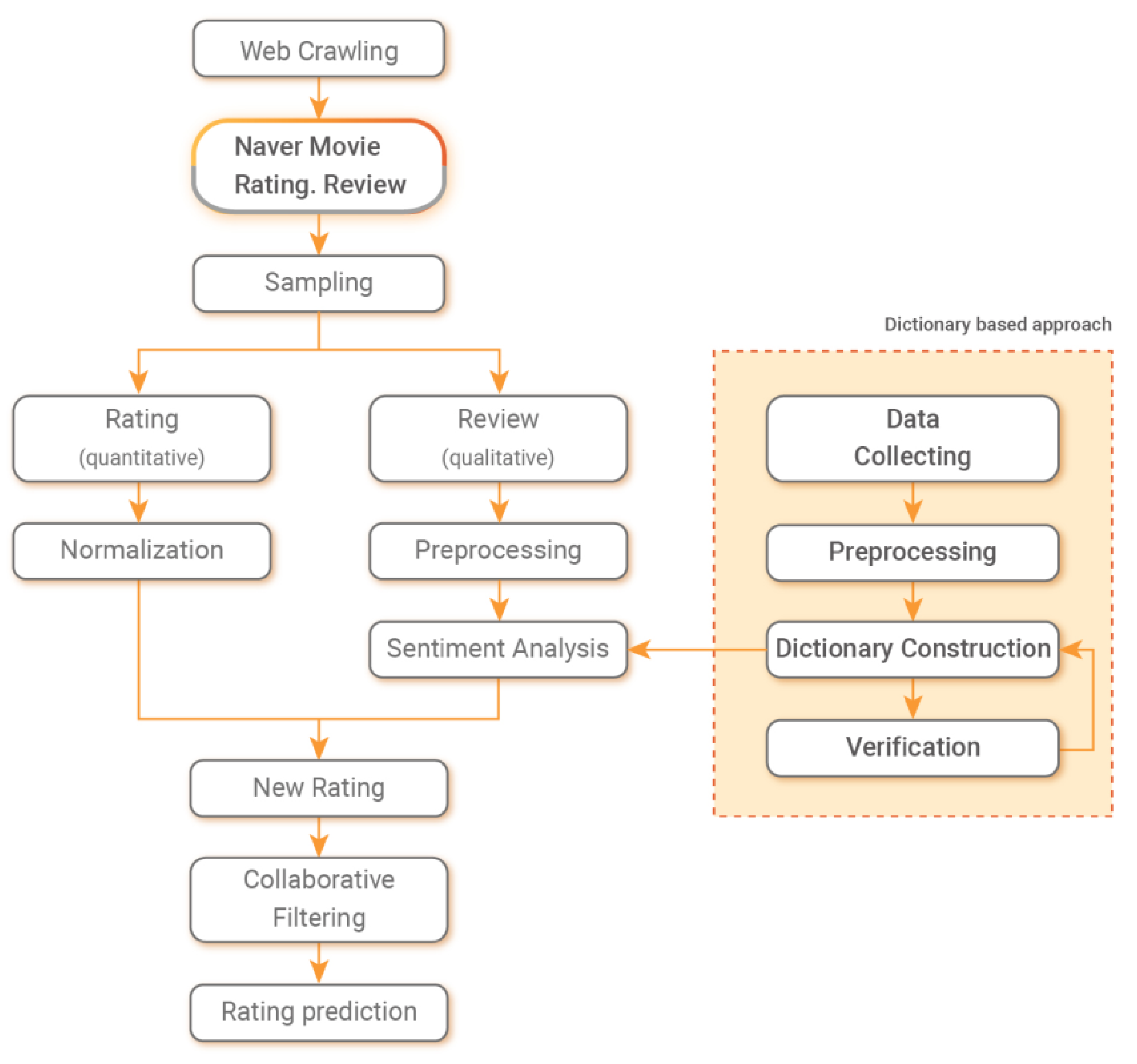
Figure 3 shows the proposed algorithm.

3.1. Step 1, Data Collection (Web Crawling)

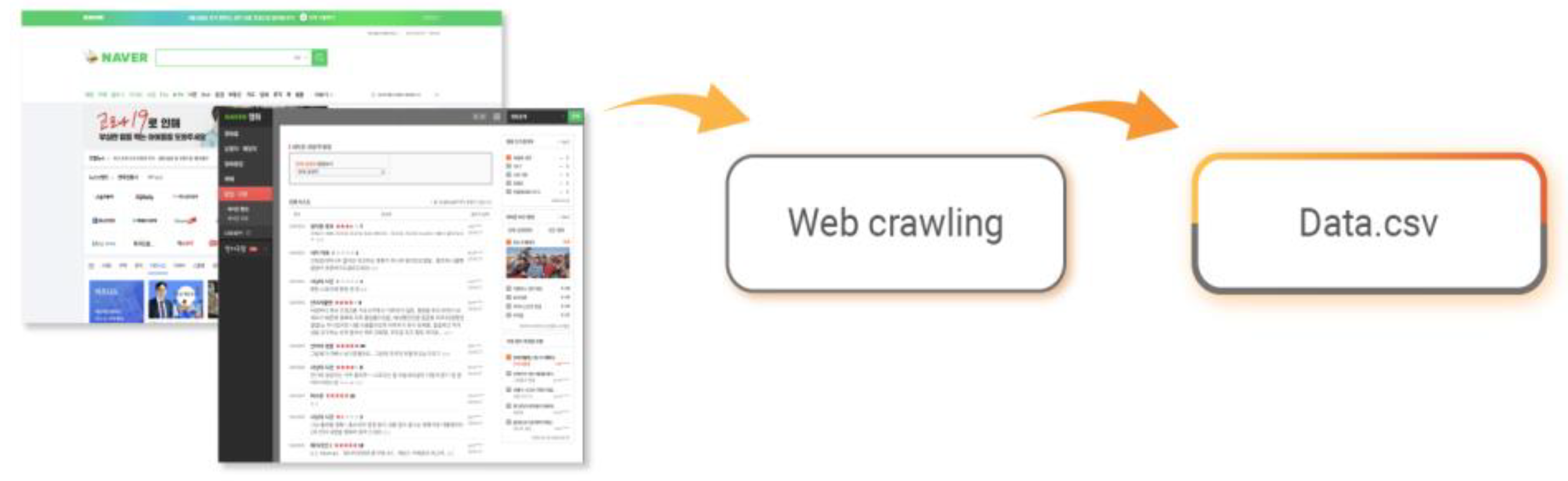
Within the texts, emotions, assessments, attitudes, facts, etc., are expressed. Among many types of texts, movie reviews were used for the analysis as they efficiently express user sentiments in short sentences of no longer than 140 characters [24]. The data were collected from NAVER Movies (movie.naver.com), which is operated by NAVER, the largest online platform in Korea. Further, a web crawling process was used to access the users and collect movie ratings and reviews left by the users.

The procedure of collecting review and rating data is shown in Figure 4. The original intent was to use the NAVER Movie API in collecting the data; however, the desired information for the study could not be collected through the API. Thus, the data were collected using a Python-based web crawler to automatically accumulate various information by visiting the website. After accessing the users through the web crawler, movie titles, ratings, and reviews left by the users were collected. The collected data consisted of 3856 users, 32,486 individual movie titles, and 100,230 movie ratings and reviews. Moreover, the rating data were in the scale of 1 to 10 points, without decimal points.

3.2. Step 2, Sampling the Data

Within the collected data, a data scarcity issue was found because the number of movies that had not been rated was greater than the number of movies that had been rated, among the entire collection of movies for which the users had left ratings and reviews. If the number of rated movies is small, incorrect similarity could be returned when finding similar users or items during the recommendation process. To reduce this data scarcity, only the users who left both ratings and reviews on at least 10 or more movies were selected for the experiment in this study. For this study, a total of 537 users and 4211 movie titles were selected from the collected data.

3.3. Step 3, Rating-Normalization

The user rating data are generally unequally distributed according to the user preferences. Owing to different criteria for rating items, there are users who generally tend to provide higher ratings, whereas other users tend to provide lower ratings. In the former case, a rating of 5 points would indicate a non-interesting movie, whereas this rating could indicate an interesting movie in the latter case. Hence, viewing the same rating scores of two different people in the same perspective cannot reflect the different rating tendencies and criteria of each person, as it could lead to a poor prediction accuracy. To reduce any bias caused from external factors, the data were normalized based on the personal evaluation tendencies of the users given that normalization can provide more accurate user similarities and user movie preferences.

In this study, we attempted to normalize user ratings by reflecting the rating tendency of users based on the differences in their preference for various items.

3.3.1. Movie Recommendation Approach Applying Differences in User Preferences or Partiality for Items

Based on user rating information, the difference or variances average rating score between items is calculated and then using it, the target user’s rating of a new item is predicted.

To calculate the differences in the preference for items, the average rating differences among the items are derived based on the item rating scores given by the users. The average user’s preference difference $d_{i,j}$ between two items i and j can be derived by using Equation (1).

$$d_{i,j}=\frac{{\sum }_{a\in U_i\cap U_j}\left(r_{a,i}-r_{a,j}\right)}{\left|U_i\cap U_j\right|}$$

(1)

In Equation (1), the terms the rating difference of two items based on the users’ evaluations are expressed as $U_i, U_j$, as $r_{a,i}-r_{a,j}$.

The preference prediction can be derived from Equation (2), which uses the average rating difference obtained from Equation (1) to derive the rating ${\widehat{r}}_{u,i}$ given by user u for the new item i.

$${\widehat{r}}_{u,i}=\frac{{\sum }_{j\in I_u}\left(r_{u,j}+d_{i,j}\right)}{\left|I_u\right|}$$

(2)

Using Equation (2), the rating that will be given by user u for the new item i is predicted based on the rating for item j. This can be achieved by adding the average preference difference $d_{i,j}$ between items i and j to user u’s rating preference $r_{u,j}$ for the rated item j. Subsequently, the predicted values obtained using item j are averaged to obtain ${\widehat{r}}_{u,i}$. This corresponds to the case where the importance for each predicted value is considered as a constant value of 1.

$${\widehat{r}}_{u,i}=\frac{{\sum }_{j\in I_u}\left\{\left(r_{u,j}+d_{i,j}\right)·\left|U_i\cap U_j\right|\right\}}{\left|I_u\right|}$$

(3)

The number of users that evaluated both items i and j, $\left|U_i\cap U_j\right|$, can be considered as the weight of item j, which can then be multiplied with Equation (2) to derive the relative importance of each item j. Equation (3) denotes the equation corresponding to the application of a weighted average.

3.3.2. Recommendation Method Applying User Rating Tendency

The accuracy of rating prediction is improved by reflecting user tendencies for determinations when rating with the recommendation method and applying the user preference differences to items.

The manner in which users decide the rating for a given item varies depending on the personal preference of each user. For example, in the case of movie ratings, when there are two users u1 and u2 who judge the rating based on the five different criteria of storyline, characters, story development, entertainment value, and cinematography, user u1 may rate a movie as 10 out of 10 as long as the movie satisfies the entertainment value criterion, regardless of other criteria. In contrast, user u2 may rate the movie as 6 out of 10 if any one of the five criteria are not satisfied. As such, the rating tendencies differ for each user depending on the user’s preference; therefore, a process for converting subjective data into more objective data is required to apply the rating data obtained from various users to predict a different user’s rating for a new item. Accordingly, if the collected rating data can be appropriately normalized based on users’ rating tendencies, a more accurate recommendation can be provided to a new user, u3. User rating normalization is the process of adjusting the data distribution of user ratings such that the entire sample data has the same median, and it is performed as follows.

1. Normalization based on a median of 5.5

Since the median rating score is 5.5 when the users can rate items on a scale of 1 to 10, the normalization is conducted based on the median value of 5.5 in order to adjust each user rating dataset distribution to have a minimum rating score of 1 and a maximum rating score of 10. For example, in the case where the maximum rating score given by user u1 is 8.0 out of 10, the process of normalizing a rating score of 7.0 given by user u1 is as follows. Since the score of 7.0 is greater than the median value of 5.5, the score is normalized by employing $5.5+\left\{\left(7-5.5\right)\times \frac{10-5.5}{8-5.5}\right\}$ to adjust the score such that it lies within the common scale of 1 to 10. The normalization of the user’s rating score considering the minimum rating score is conducted similarly. For example, when the minimum rating score given by a user is 2.0, the user’s rating score of 3.0 can be normalized by adjusting the score to the common scale using $5.5-\left\{5.5-3\times \frac{5.5-1}{5.5-2}\right\}$.

2. Normalization of Data Between Median and Minimum in the Rating Value Range

When the range of a user’s rating data is within the range constituted by the minimum value and median value of the common scale only, the maximum value of the user rating is set as the median value of the common rating scale, 5.5. Additionally, the minimum value of the user rating is set as the minimum value of the common rating scale, 1. Subsequently, normalization is conducted based on the median value of this user rating range, which is 3.25.

3. Normalization of Data Between Median and Maximum Rating Value Range

Similar to the case described in 2, when the range of a user’s rating data is localized such that it lies between the maximum and median rating values of the common scale only, the maximum value of the user rating is set as the maximum value of the common rating scale. Additionally, the minimum value of the user rating is set as the median value of the common rating scale, and normalization is performed based on the median value of this user rating range, which is 7.75.

Based on the recommendation method that uses the user preference differences among various items, user rating normalization is applied according to the rating decision tendencies of users. The normalized rating data are applied to Equation (1). Through Equation (1), by using the rating data of users who rated both items i and j, the user rating differences for items i and j are aggregated. During this process, the rating data that have been normalized according to the individual user rating tendency for items i and j can serve as a more objective index in predicting the target user’s rating.

After normalizing the selected user rating data, the extracted normalized rating data from the users were transformed into a user x item rating matrix, with user, item, and rating relations, as shown in

Table 1. Example of user-item rating matrix.

	Item1	Item2	Item3	…	Item M
User 1	2	?	4		1
User 2	?	8	6		?
User 3	2	?	?		7
…
User N	1	5	4		2

[25].

3.4. Step 4, Review-Preprocessing

Before conducting morphological analysis, which allows a more accurate review data analysis, words that do not have meanings, special characters, punctuation marks, English words, numbers, etc., were removed. Subsequently, morphological analysis was conducted to extract the necessary parts of speech of the reviews. Among various morphological analyzers, the RHINO library, which is a Korean morphological analyzer, was used to select and extract only the nouns, verbs, and adjectives that are most frequently used in sentiment analysis.

3.5. Step 5, Review-Sentiment Analysis

3.5.1. Step 5-1, Review Data Collecting

In constructing the sentiment dictionary, data from NAVER Lab were used as additional data. A total of 200,000 review data were obtained, which had rating integer values between 1 and 10. If the rating score was from 1 to 3, a label of 0 (negative) was assigned to the review, and if the rating score was from 9 to 10, a label of 1 (positive) was assigned. Among the data, 100,000 reviews were extracted with an equal polarity ratio of negative and positive labels. Subsequently, 75,000 movie reviews were used to construct the dictionary and 25,000 movie reviews were used as test data to verify the accuracy of the dictionary.

3.5.2. Step 5-2, Review Data Preprocessing

Morphological analysis was carried out using the same four-step pre-processing procedure. After the morphological analysis, the RHINO library was used to select and extract only the nouns, verbs, and adjectives of the parts of speech from the review data.

To construct a sentiment dictionary, words and phrases were extracted from the training data. In this study, the adjective, noun, and verb parts of speech tags that directly describe and express sentiments, were extracted from the training data to construct word and classification graphs. Among these, the ones that clearly express emotions were defined as sentiment words and sentiment phrases.

Table 2. The number of extracted words and phrases.

Words				Phrases
Noun (NNG)	Verb (VV)	Adjective (VA)	Total	2430
1017	296	81	1394

shows the number of words and phrases extracted to construct the word and phrase graphs, and

Table 3. The examples of pre-defined sentiment words.

Sentiment (Count)	Sentiment Words
Positive (14)	good/VA, fun/VA, fine/VA, sad/VA, like/VV, funny/VA, pretty/VA, stand out/VV, sad/VA, amaze/VV, appeal/NNG, awesome/VA, heartbreaking/VA, strong recommendation/NNG
Negative (14)	awkward/VA, fall for/VV, tedious/VA, worst/NNG, annoy/VV, irritating/NNG, rowdy/VA, obvious/VA, disturb/VV, be criticized/VV, bad/VA, embarrassing/VV, boring/VA, unpleasant/VA

;

Table 4. The examples of pre-defined sentiment phrase.

Sentiment (Count)	Sentiment Phrases
Positive (30)	(expectation/NNG, high/VA), (scene/NNG, sad/VA), (movie/NNG, heartbreaking/VA), (impress/NNG, be/VV), (storyline/NNG, decent/VA), (tears/NNG, fall/VV)
	(thriller/NNG, is/VV), (portrayal/NNG, stand out/VV), (goosebumps/NNG, rise/VV), (love/NNG, overflow/VV), (perfect score/NNG, give/VV), (stress/NNG, relieve/VV), (inspiration/NNG, deep/VA)
Negative (30)	(expectation/NNG, different from/VA), (movie/NNG, exaggerate/VV), (money/NNG, waste/VA), (constraint/NNG, overdo/VV), (impression/NNG, weak/VA), (time/NNG, waste/VA), …
	(hands and feet/NNG, cringe/VV), (feeling/NNG, crap/VA), (suspense/NNG, lack/VA), (unreality/NNG, excessive/VA), (immersion/NNG, difficult/VA), (imagination/NNG, no/VA), (limit/NNG, feel/VV)

each display the defined words and phrases.

3.5.3. Step 5-3, Dictionary Construction

The pre-processed review data were transformed into a document-term matrix. During this process, the Term frequency inverse document frequency (TF-IDF) weight method, which indicates the importance and frequency of the word in a document, was used to vectorize the texts.

Figure 5 displays the sentiment dictionary construction flow chart.

The independent variables are the TF-IDF value matrix of review words and the dependent variables are the label values of 0 and 1 of each review. Regression analyses were used to construct the dictionary. After acquiring regression coefficients of each word, the sentiment dictionary was constructed by placing the words into the positive dictionary if the coefficient was greater than 0 and into the negative dictionary if less than 0. However, as the text data lacked structures and had a large number of dimensions, the process of selecting and extracting variables when conducting regression analysis is important to improve the analysis performance. Thus, Ridge, Lasso, and ElasticNet regressions were used among the regression methods [26].

Ridge regression is a method of shrinking the regression coefficient by penalizing the regression model with a penalty [27]. Ridge regression is a linear regression that has $L_2$- constraints. The ridge estimates are obtained using Equation (4).

$${\widehat{\beta }}_{ridge}=agrmin\left\{{\displaystyle \sum }_{i=1}^N{(y_i-{\beta }_0-{\displaystyle \sum }_{j=1}^P{x}_{ij{\beta }_j})}^2+\lambda {\displaystyle \sum }_{j=1}^P{\beta }_j^2\right\}$$

(4)

From the equation, $\mathsf{\lambda }\left(\mathsf{\lambda }\ge 0\right)$ determines the amount of shrinkage of the regression coefficient. As the $\mathsf{\lambda }$ value increases, the shrinkage amount also increases, and the regression coefficient value tends to zero.

Lasso regression analysis is a method of shrinking the regression coefficient by penalizing the regression model with a penalty, similar to ridge regression analysis [28]. This estimation method enables variable selection by making regression coefficient values of insignificant variables, as the lasso estimates are obtained using Equation (5).

$${\widehat{\beta }}_{lasso}=argmin\left\{{\displaystyle \sum }_{i=1}^N{(y_i-{\beta }_0-{\displaystyle \sum }_{j=1}^P{x}_{ij}{\beta }_j)}^2+\lambda {\displaystyle \sum }_{j=1}^P\left|{\beta }_j\right|\right\}$$

(5)

As the value of $\mathsf{\lambda }\left(\mathsf{\lambda }\ge 0\right)$ in Equation (2) increases, the value of the regression coefficient tends to zero.

The main difference between the two models of the ridge regression and lasso regression is that the ridge model uses the square of the coefficients; however, the lasso model uses the absolute value. Because the coefficients of each independent variable are close to zero, but not actually zero, the ridge model employs all the independent variables, even if the penalty value is large. However, because some variables become zero if the penalty value is large, the lasso model employs only the selected variables that are not zero.

ElasticNet is an algorithm that combines both ridge and lasso regressions. The ElasticNet estimates are obtained by Equation (6).

$${\widehat{\beta }}_{ElasticNet}=argmin\left\{{\displaystyle \sum }_{i=}^N{(y_i-{\beta }_0-{\displaystyle \sum }_{j=1}^P{x}_{ij}{\beta }_j)}^2+\lambda \left[\alpha {\displaystyle \sum }_{j=}^P\left|{\beta }_j\right|+\left(1-\alpha \right){\displaystyle \sum }_{j=1}^P{\beta }_j^2\right]\right\}$$

(6)

The ElasticNet linearly adds penalties of the ridge and lasso methods and adjusts $\mathsf{\lambda }$ to derive an optimized model. Additionally, it adds an extra parameter of α to differentiate the relationship between the two. In contrast to the ridge and lasso methods, which are adjusted with $\mathsf{\lambda }$, parameter α is employed, and the lasso effect increases with an increase in the value of α, whereas the ridge effect increases with the decrease in the value of α.

When using the ridge, lasso, and ElasticNet regression methods, a cross-validation method was used to estimate the shrinkage parameter $\mathsf{\lambda }$. After obtaining the optimal $\mathsf{\lambda }$ value that returns the smallest error through fivefold cross validation, the word that has a regression coefficient value greater than 0 for the given $\mathsf{\lambda }$ value was classified into the positive dictionary, and the word with a value less than 0 was classified into the negative dictionary, thereby constructing a positive and a negative dictionary.

The words of each constructed dictionary were manually checked and any unnecessary words were removed. For example, if the dictionary contained nouns that were not related to sentiments, such as actor’s names, location names, etc., the corresponding words were removed.

3.5.4. Step 5-4, Dictionary Accuracy Verification

In verifying the accuracy of the dictionary, a test dataset of 25,000 review data was used. Based on the dictionary, sentiment scores of reviews were calculated and classified as positive if the sentiment score was greater than 0, and as negative if less than 0. The sentiment scores are obtained through Equation (7).

$$\mathrm{Sentiment} \mathrm{Score}=\frac{Posword-Negword}{Posword+Negword}$$

(7)

To examine the accuracy of the sentiment dictionary, sentiment scores are calculated based on the frequency of the positive and negative words. The sentiment score can range from negative 1.0 to positive 1.0. The words that fall in the score range of +0.1 to +1.0 are identified as positive words, while the words that fall in the range of -1.0 to -0.1 are identified as negative words. Subsequently, the sentiment scores obtained through sentiment analysis are applied to the rating data and new ratings are generated.

As a measure to evaluate the positive and negative prediction results, misclassification ratio was used, and by measuring the accuracy of the confusion matrix of

Table 5. 2 × 2 Confusion matrix.

	Actual Positive	Actual Negative
Predicted Positive	TF(True Positive)	FP(False Positive)
Predicted Negative	FN(False Negative)	TN(True Negative)

, dictionaries with high performance were selected for the analysis [29].

In this matrix, the values of TP(True Positive), FP(False Positive), TN(True Negative), and FN(False Negative) represent the result values.

TP indicates that the classifier accurately predicted by classifying the positive case as a positive. Conversely, FP indicates that the classifier incorrectly classified the negative case as positive. Similarly, TN denotes that the classifier accurately predicted by classifying the negative case as a negative, while FN denotes that the classifier incorrectly classified the positive case as a negative. Based on the results derived from the confusion matrix, accuracy, precision, and recall can be derived. Equations (8)–(11) respectively express the equations for calculating the accuracy, recall, precision, and F-measures.

$$\mathrm{Accuracy}=\frac{TP+TN}{TP+FP+TN+FN}$$

(8)

$$\mathrm{Precision}=\frac{TP}{TP+FP}$$

(9)

$$\mathrm{Recall}=\frac{TP}{TP+FN}$$

(10)

$$\mathrm{F}-\mathrm{measure}=\frac{2\times \left(Precision\times Recall\right)}{\left(Precision+Recall\right)}$$

(11)

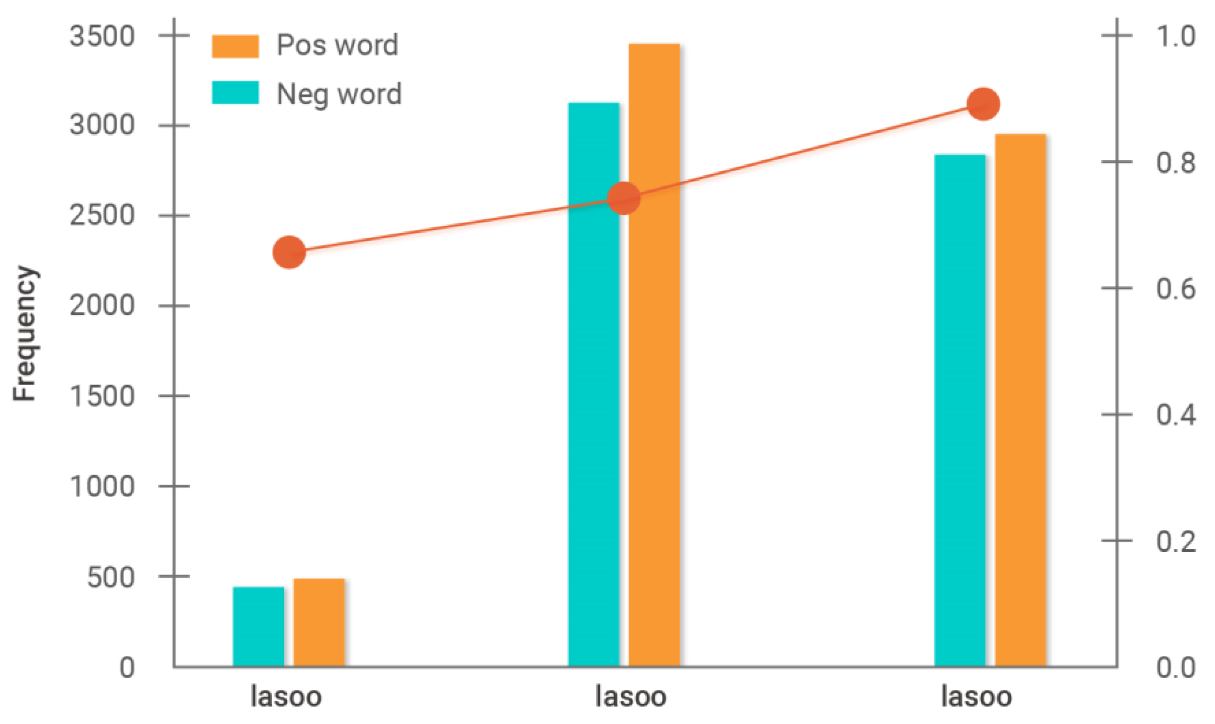
Figure 6 displays the results of calculating the accuracy based on the positive and negative vocabulary frequency of each dictionary and on Equations (7) and (8). Based on the results of the number of words used in the dictionary, the words were more diverse in the way of expressing negative vocabulary than expressing positive vocabulary.

The lasso-based dictionary featured 398 positive sentiment vocabulary and 421 negative sentiment vocabulary, with 70% accuracy. The ridge-based dictionary featured 3164 positive sentiment vocabulary and 3425 negative sentiment vocabulary, with 79% accuracy. When constructing the ElasticNet-based dictionary, α of 0.3 was chosen as it returned the highest accuracy. A total of 2875 positive and 2954 negative vocabulary was extracted with 83% accuracy. As a result, this study used an ElasticNet-based positive and negative dictionary, which had the highest accuracy, for calculating the sentiment scores of user reviews.

Furthermore, this study used the SVM (support vector machine), RF (random forest), and NNet (neural network) algorithms, which are popular methods for recognizing and classifying sentiments. The training and test data were labeled according to the collected sentiment words in the sentiment dictionary. Furthermore, the classifier models were trained using the training data and the trained models were used to classify the sentiments of the test data. The SVM model used a traditional kernel function RBF (radial basis function); the RF model used a total of 500 trees with 10 variables; the NNet used a total of 10 hidden layers. Then, similarly to the earlier regression analysis method of this paper, the 5-fold cross-validation method was used for the classification performance test. For performance measurement, recall, precision, and F-measures were selected to test the accuracy of the model

Table 6. The results of sentiment analysis for movie reviews using the proposed sentiment dictionary.

Classifier	Evaluation Measures	Classification Performance (%)
		General Dictionary	Proposed Dictionary
RF	Recall	86.76	71.95
	Precision	57.28	85.51
	F-measure	69.01	78.15
SVM	Recall	86.76	62.2
	Precision	55.66	93.1
	F-measure	67.82	74.57
Nnet	Recall	66.18	85.37
	Precision	54.88	78.65
	F-measure	60	81.87

displays the classification performance of each classifier on the sentiment dictionary.

The results of using the general sentiment dictionary and the domain-specific dictionary constructed for analysis identified the following distinctions. Except for the analysis results of the NNet model, the recall values were generally higher than the precision values when using the general dictionary, while the precision values were higher than the recall values when using the sentiment dictionary. Additionally, the dictionary returned a higher F-measure due to the smaller difference between the recall and precision than did the general sentiment dictionary. These results suggest that the constructed dictionary yielded a more stable and accurate sentiment analysis result.

3.6. Step 6, New Rating Peflecting Sentiment Digitization

The sentiment scores of the entire text data were numerically expressed based on the positive and negative words featured in the constructed sentiment dictionary. The sentiment scores are derived using Equation (7). The sentiment scores obtained through the sentiment analysis are reflected in the rating data to generate a new rating data. An example of the generated rating is shown on the right side of

Table 7. Original ratings and proposed new ratings.

	Item 1	Item 2	Item 3	…	Item M		Item 1	Item 2	Item 3	…	Item M
User 1	2	?	5		9	User 1	2.24	?	4.48		9.45
User 2	?	7	6		?	User 2	?	7.75	6.21		?
User 3	5	?	?		3	User 3	4.48	?	?		2.98
…						…
User N	?	5	?		4	User N	?	5.12	?		4.34

. Although previous user ratings used integer values, from 1 to 10, the newly generated ratings of the proposed method use real numbers.

3.7. Step 7, Rating Prediction

In predicting user ratings, user-based and item-based filtering of model-based collaborative filtering and SVD and SVD++ algorithms, which are popular algorithms of model-based matrix factorization, were used.

After selecting neighboring users who have similar preferences as the target user, based on the rating information entered by the user, user-based collaborative filtering is a method of providing recommendations to a user with items that are commonly preferred by neighboring users. The most important step in predicting ratings through user-based collaborative filtering is calculating the user similarities. The similarity between the two users a and b, $Similarit{y}_{\left(a,b\right)}$, is obtained by Equation (12).

$$Similarit{y}_{a,b}=\frac{{\sum }_{i\in I}\left(r_{a,i}-{\overline{r}}_a\right)\left(r_{b,i}-{\overline{r}}_b\right)}{\sqrt{{\sum }_{i\in I}{\left(r_{a,i}-{\overline{r}}_a\right)}^2}\sqrt{{\sum }_{i\in I}{\left(r_{b,i}-{\overline{r}}_b\right)}^2}}$$

(12)

Here, I denotes the entire set of items, $r_{a,i}$ denotes the rating score given by user a on item $\mathrm{i}$, and ${\overline{r}}_a$ indicates the average rating score of all items that user a has rated. Once the users with similar preferences are selected through the similarity measure, the user rating is predicted based on their purchase history, using the weighted sum method.

The predicted rating that user $\mathrm{a}$ would provide on the item i is obtained through Equation (13).

$${\widehat{r}}_{a,i}={\overline{r}}_a+\frac{{\sum }_{u\in U}\left(r_{u,i}-{\overline{r}}_u\right)\times W_{a,u}}{{\sum }_{u\in U}\left|W_{a,u}\right|}$$

(13)

Further, ${\overline{r}}_a$ indicates the average score of all items given by the recommendation target user, ${\overline{r}}_u$ denotes the average score of all items given by the other user, and $W_{a,u}$ represents the weight of the similarity between the user u and recommendation target user a, where a higher similarity returns a larger weight.

In the item-based collaborative filtering, a specific item is selected as a standard, and then a neighboring item with similar user rating scores is selected. Consequently, based on the neighboring item rating score, a rating that the target user might have for the specific item is predicted. The similarity between the two items $\mathrm{i}$ and $\mathrm{j}$, $Similarit{y}_{\left(i,j\right)}$ is obtained by Equation (14).

$$Similarit{y}_{i,j}=\frac{{\sum }_{u\in U}\left(r_{u,i}-{\overline{r}}_i\right)\left(r_{u,j}-{\overline{r}}_j\right)}{\sqrt{{\sum }_{u\in U}{\left(r_{u,i}-{\overline{r}}_i\right)}^2}\sqrt{{\sum }_{u\in U}{\left(r_{u,j}-{\overline{r}}_j\right)}^2}}$$

(14)

Here, U indicates the set of all users who rated both items $\mathrm{i}$ and $\mathrm{j}$, $r_{u,i}$ represents the score on item $\mathrm{i}$ given by user u, and ${\overline{r}}_i$ represents the average score on item $\mathrm{i}$ given by all users.

The item-based collaborative filtering predicts rating scores through a simple weighted average method, as shown by Equation (15).

$${\widehat{r}}_{u,i}=\frac{{\sum }_{n\in N}\left(r_{a,n}\times W_{i,n}\right)}{{\sum }_{n\in N}\left|W_{i,n}\right|}$$

(15)

Here, ${\overline{r}}_a$ and ${\overline{r}}_u$ denote the average score of all items given by the recommendation target user and the other user, respectively. Further, $W_{i,n}$ uses the weighted similarity between the item to be predicted and the other item to calculate the prediction value by reflecting the rating of the similar item to the item to be predicted.

Among the model-based matrix factorization methods, SVD and SVD++ are the most widely used methods in collaborative filtering. SVD is a method of decomposing a matrix into a product of any matrices. A singular value decomposition on matrix M, $\mathrm{m}\times \mathrm{n}$, of all users and items can be expressed as the product of three matrices, as shown by Equation (16).

$$\mathrm{M}=\mathrm{U}\sum V^T$$

(16)

In the equation, $U_{m\times n}$ denotes a user matrix, $\sum m\times n$ denotes the diagonal matrix entries with singular values in diagonal terms, and $V_{n\times n}^T$ represents a movie matrix.

However, as the matrix M is a sparse matrix, there is a probability that SVD may not be defined, owing to many empty values (missing values) that are not provided by the user. To address this problem, a normalized model, Equation (11), is used to predict the rating by deriving a factor vector that minimizes the error function, based on the ratings given by the user.

$$\min {\sum }_{\left(u,i\right)\in M}{\left(r_{ui}-{\widehat{r}}_{ui}\right)}^2+\lambda \left(\Vert q_i\Vert {}^2+\Vert p_u\Vert {}^2\right)$$

(17)

For the method of minimization, SGD is used to calculate the prediction error, and by adjusting the parameters, ${\widehat{r}}_{ui}$ can be predicted through Equations (18) and (19).

$$q_i\leftarrow q_i+\lambda \left(\left(r_{ui}-q_i^T\right)p_u-\lambda q_i\right)$$

(18)

$$p_u\leftarrow p_u+\lambda \left(\left(r_{ui}-q_i^T\right)q_i-\lambda p_u\right)$$

(19)

In contrast to SVD, which considers explicit feedback information only, the SVD++ method considers both implicit and explicit feedback information.

Based on the SVD method, the characteristics of all the items are reflected in SVD++, regardless of having user rating scores or not. The rating prediction using the SVD++ method is obtained using Equation (20).

$${\widehat{p}}_{ui}=\mu +b_u+b_i+q_i^T\left(p_u+{\left|R\left(u\right)\right|}^{-\frac{1}{2}}\sum _{j\in R\left(u\right)}{y}_j\right)$$

(20)

The rating prediction value ${\widehat{r}}_{ui}$ can be derived by the sum of $\mathsf{\mu }$ and $b_u$, $b_i$, which is the average rating of all data and individual bias values on users and items, respectively. To include the additional association between the user and the item, the explicit rating data matrix and the implicit rating data matrix were decomposed based on SVD. Subsequently, by searching for a low-dimensional hidden space that collectively expresses both the user and item, d-dimensional latent vectors $q_i$ for the item and $p_u$ for the user, were obtained. $\mathrm{R}\left(u\right)$ is characterized by the user, with preference on the item, as a vector. $y_j$ is an attribute that describes the user u.

4. Performance Evaluation Method and Experiment Results

4.1. Performance Evaluation Method

To examine the difference between the recommendation system method reflecting only the rating data and the method integrating the rating data with sentiment scores, the mean absolute error (MAE) and root-mean-square error (RMSE) are used for the evaluation method. The two measures, which help show the difference between the predicted user rating and the actual user rating, are the most frequently used measures in the recommendation systems using collaborative filtering [30,31].

MAE is defined as shown in Equation (21).

$$\mathrm{MAE}=\frac{{\sum }_{ij}\left|R_{ij}-{\widehat{R}}_{ij}\right|}{N}$$

(21)

RMSE is defined as shown in Equation (22).

$$\mathrm{RMSE}=\sqrt{\frac{{\sum }_{ij}{\left(R_{ij}-{\widehat{R}}_{ij}\right)}^2}{N}}$$

(22)

Here, N indicates the number of data points; $R_{ij}$ denotes the actual rating on item j, given by the user $\mathrm{i}$; and ${\widehat{R}}_{ij}$ denotes the rating prediction that the user might provide. MAE is a mean absolute error measure that is calculated by adding all the absolute values of the errors between the measured value and the predicted value and dividing it by the number of predicted values. Meanwhile, RMSE is as RMSE measure calculated by first obtaining the sum of the squared differences between the actual and predicted values and then dividing the sum result by the number of predictions, followed by the square root. In both these measures, smaller error values indicate a better prediction accuracy of the recommendation system.

4.2. Experiment Results

Using the described MAE and RMSE, the performances of the existing method using only ratings for prediction and the prediction method proposed in this paper were compared. For the data, 80% was used as training data, and 20% as test data. Further, cross-validation was conducted to evaluate the rating prediction performances. The experimental results of fivefold cross-validation, using the user-based collaborative filtering algorithm, are shown in

Table 8. User-based collaborative filtering mean absolute error (MAE)/root-mean-square error (RMSE).

Title 1	Original Rating		Proposed New Rating
Test #	MAE	RMSE	MAE	RMSE
1	2.3051	3.0656	2.2817	3.1120
2	2.2964	3.1229	2.2273	3.0731
3	2.3310	3.0303	2.2178	3.0231
4	2.2743	3.1152	2.2923	2.9964
5	2.3185	3.0675	2.2021	2.9667
Avg.	2.3056	3.0803	2.2442	3.0342

.

The “Original Rating” represents the basic performance of the system, reflecting only the rating, whereas the “Proposed Rating” represents the performance of the proposed method, which reflects the sentiment scores in predicting the user rating.

The user-based collaborative filtering returned a MAE value of 2.3056 and RMSE value of 3.0803 for the Original Rating and a MAE value of 2.2442 and RMSE value of 3.0342 for the Proposed Rating. The MAE improved by 0.0614 and RMSE by 0.0461 in the proposed method.

The results of the item-based collaborative filtering are shown in

Table 9. Item-based collaborative filtering MAE/RMSE.

Title 1	Original Rating		Proposed New Rating
Test #	MAE	RMSE	MAE	RMSE
1	2.1514	2.8701	2.045	2.8025
2	2.1333	2.8812	2.0211	2.8062
3	2.0954	2.9122	2.012	2.781
4	2.103	2.858	2.0451	2.8175
5	2.1173	2.9009	2.0608	2.8003
Avg.	2.1201	2.8845	2.0368	2.8015

, where the MAE improved by 0.0833 and the RMSE by 0.083, compared to the existing method of reflecting only the rating data.

Table 10. Singular value decomposition (SVD) MAE/RMSE.

Title 1	Original Rating		Proposed New Rating
Test #	MAE	RMSE	MAE	RMSE
1	1.9898	2.6216	1.8727	2.4924
2	1.9778	2.6147	1.8984	2.5038
3	1.9356	2.6021	1.8755	2.4563
4	1.9736	2.6174	1.8683	2.5134
5	1.9801	2.6122	1.8536	2.4976
Avg.	1.9714	2.6136	1.8723	2.4928

displays the MAE and RMSE results of the SVD algorithm. In this study, to confirm that the optimized prediction by combining sentiment scores with rating data yields a higher accuracy than the method reflecting only the rating data, the prediction accuracies were measured under the same conditions. The result indicates that the MAE value improved by 0.0991 and the RMSE improved by 0.1208.

Table 11. SVD++ MAE/RMSE.

Title 1	Original Rating		Proposed New Rating
Test #	MAE	RMSE	MAE	RMSE
1	1.9514	2.6302	1.7802	2.4964
2	1.8772	2.6473	1.7432	2.5213
3	2.0354	2.6524	1.7556	2.4628
4	1.9559	2.6319	1.8250	2.4499
5	1.9989	2.6482	1.7168	2.3213
Avg.	1.9638	2.6419	1.7602	2.4503

displays the MAE and RMSE results of using the SVD++ algorithm. The proposed method of combining sentiment scores showed a MAE improvement of 0.2036 and RMSE improvement of 0.1916.

Table 12. Experiment results of proposed model with test data.

		MAE		REMS
		Original	Proposed	Original	Proposed
Memory-based CF	UBCF	2.3013	2.2417	3.0867	3.0426
	IBCF	2.0984	2.0122	2.8946	2.8064
Model-based CF	SVD	1.9754	1.8742	2.6146	2.5043
	SVD++	1.9625	1.7745	2.6228	2.4532

shows the performance results of the proposed method using the test data.

For the MAE measures of the test data evaluation, the user-based and item-based collaborative filtering methods obtained MAE improvements of 0.059 and 0.0862, respectively, while the SVD and SVD++ algorithms showed improvements of 0.1012 and 0.188, respectively. For the RMSE measures, the user-based and item-based collaborative filtering methods showed improvements of 0.0431 and 0.0882, respectively, and the SVD and SVD++ algorithms showed improvements of 0.1103 and 0.1756, respectively. The analysis results suggested that the proposed method of reflecting the sentiment scores in the rating prediction yields significantly better overall prediction performance than the existing method of reflecting only the rating data.

The model that showed the highest performance improvement among the existing method of reflecting only the rating data was SVD++. The proposed method of reflecting sentiment scores obtained better rating prediction accuracies in all methods. In particular, as shown in Table 8, the model-based collaborative filtering performed better than the memory-based collaborative filtering method. This may be due to the use of a sparse matrix, an environment in which the model-based algorithms would return more accurate user ratings. There are two main drawbacks in using data of sparse matrices: The first issue is the cold start problem. This issue occurs when the rating cannot be predicted, owing to the lack of data to measure the similarity, from users who have not entered a single user rating. The second issue is the first rater problem. This issue occurs when there is an item that no one has purchased before, resulting in no recommendation made until some user provides a rating on the item.

In this study, the cold start problem was avoided by limiting the data to users who have rated and wrote reviews on at least 10 movies. Furthermore, the first rater problem was eliminated by collecting the movie title, rating, and review data on a user basis. Thus, all the movies had at least one or more ratings. Nonetheless, data were insufficient because the number of movies that the users have rated was less than the total number of movie titles. Hence, the probability of locating users with similar preferences in the items to the target user was low, resulting in a relatively low performance of the memory-based recommendation system compared with the model-based system. However, the model-based collaborative filtering method deviates from simply comparing the similarity between the users or items. Instead, it uses the patterns and attributes that are implied in the data. Hence, the user rating on a specific item can be predicted, even without the rating information. It is assumed that the SVD method acquired better performance in the user rating prediction by reducing the dimensions of the matrix by directly removing insignificant users or items from the matrix. Thus, data scarcity issue and noise were reduced.

4.3. Evaluation Method Using Feature Selection Approach

In this study, feature selection was not applied to the TF-IDF generated at the preprocessing stage; rather, the feature selection method was used to improve prediction performance. Feature selection is often used in data mining to increase prediction performance and efficiency by reducing the data dimension and the required time and cost. Feature selection is advantageous for reducing the complexity of the model with minimal information loss and performance accuracy being maintained at the requisite level. The feature selection process performed for the model construction is capable of impacting the model accuracy, where, if the features are incorrectly selected, the prediction accuracy of the model may drastically decrease. This also suggests that removing unnecessary features is beneficial as they can be the factors of hindering both effectiveness and efficiency in the sentiment classification.

In this study, ElasticNet, SVM, and Naïve Bayes models were constructed without conducting feature selection on the TF-IDF generated at the preprocessing stage. The feature selection models that use weighting techniques were constructed by selecting the relevant sub-features based on the feature weights. This technique allows the use of different weights to select the sub-features. Additionally, several weight thresholds were tested to find the optimal one. The feature weighting process was conducted using various weighting methods such as SVM, Information Gain, Information Gain Ratio, principal component analysis (PCA), and chi-squared statistical weighting. In addition, by gradually changing the weighting from 0 to 0.9 at 0.1 intervals, the results of each method were compared for different weight configurations.

4.3.1. Results of Simple Modeling Techniques

Table 13. Basic model classification performance.

	ElasticNet	SVM	Naïve Bayes
Accuracy	79	80	75
AUC	85	88	63
Precision	66	55	90
Recall	76	89	63
F-measure	71	68	74

shows the performance of the models generated with ElasticNet, SVM, and Naïve Bayes algorithms without conducting feature selection on the dataset. The SVM model performed better than did the other algorithms in terms of accuracy, AUC (Area Under Curve), and precision, whereas the Naïve Bayes model performed better than the other algorithms in terms of recall. Furthermore, compared to the other algorithms, the Naïve Bayes model showed significantly poorer performance in AUC and precision.

4.3.2. Sentiment Classification Results of the Feature Selection Models Using Weighting Techniques

1. Distribution of Terms Based on Feature Weighting

Table 14. Weight by variable.

SVM	Wgt	Info Gain	Wgt	Gain Ratio	Wgt	PCA	Wgt	Chi	Wgt
Waste	1.00	Worst	1.00	Worst	1.00	Really	1.00	Waste	1.00
Worst	0.99	Waste	0.97	Worst Movie	0.84	Too	0.76	Worst	0.91
Fun	0.98	Rating	0.76	No fun	0.82	Fun	0.13	Rating	0.84
Rating	0.89	Love	0.50	Garbage Movie	0.77	Impression	0.09	Impression	0.45
Director	0.78	Impression	0.44	Nuclear no run	0.75	Waste	0.07	Probability	0.44
Boring	0.77	Probability	0.43	Waste	0.75	Movie Rally	0.06	Love	0.42
Disappointment	0.74	Garbage	0.37	Movie Worst	0.74	Rating	0.06	Just	0.42
No fun	0.66	Worst Movie	0.36	Childish	0.74	Love	0.06	Director	0.39
No	0.64	Just	0.35	Actor Waste	0.74	Time	0.06	Garbage	0.38
Just	0.60	Best	0.32	Comment	0.73	Worst	0.04	Story	0.33

shows the top term-lists based on the normalized weight assigned to each word or phrase term using the feature weighting technique. As shown in the table, although the terms like ‘waste’ and ‘worst’ appear in all lists, a difference in the top terms is observed depending on which weighting technique is applied. When examining the degree of change in weight, the PCA method tends to have a rapid drop in the normalized feature weights while the SVM and gain ratio methods tend to have lesser drops in the normalized feature weights.

Depending on the weighting method applied, the experimental results showed significant differences in the distribution of the weighted terms. In the case of the Gain Ratio weighting, the distribution was similar to the normal distribution, whereas the PCA weighting had most terms located between the 0 and 0.1 weights, and other weighting methods also exhibited higher term appearances in the lower weights. These distribution results suggest that the sentiment classification results will vary depending on the weighting method used.

2. Sentiment Classification Performance of Feature Weighting Models

The following displays the sentiment classification accuracy, AUC, precision, recall, and F-measure obtained with the ElasticNet, SVM, and Naïve Bayes feature selection models using various weighting methods. Each row denotes a different weight threshold value configuration and based on the modeling, the results were derived using the terms with normalized weights greater than or equal to the weight threshold configuration.

In the ElasticNet feature selection model with SVM weighting, high performance was observed in most performance indices when the weight threshold was greater than or equal to 0.2 (>=0.2). Conversely, in the SVM feature selection model, high performance was observed in most performance indices when the weight threshold was greater than or equal to 0.1 (>=0.1). Lastly, in the Naïve Bayes feature selection model, the weight threshold value for the highest performance for each performance index was not consistent. When comparing the three feature selection algorithms, the best overall performance was observed when the SVM weight threshold was set to 0.2 or greater, in the ElasticNet algorithm.

Table 15. ElasticNet classification performance (support vector machine (SVM) weight).

Weight	0	0.1	0.2	0.3	0.4	0.5	0.6	0.7	0.8	0.9
Accuracy	79	83	84	80	77	73	70	69	67	66
AUC	85	89	90	83	75	72	65	63	60	58
Precision	66	71	69	61	50	43	32	29	21	15
Recall	76	82	88	82	83	79	80	77	79	83
F-measure	71	76	77	70	63	56	45	42	34	26

,

Table 16. SVM classification performance (SVM weight).

Weight	0	0.1	0.2	0.3	0.4	0.5	0.6	0.7	0.8	0.9
Accuracy	80	80	80	78	74	73	69	69	68	65
AUC	88	89	87	83	75	71	64	64	61	57
Precision	55	58	53	48	39	35	26	26	22	15
Recall	89	88	91	92	90	88	88	85	85	81
F-measure	68	70	67	63	54	50	40	40	35	25

and

Table 17. Naïve Bayes classification performance (SVM weight).

Weight	0	0.1	0.2	0.3	0.4	0.5	0.6	0.7	0.8	0.9
Accuracy	75	81	80	77	77	73	69	69	67	66
AUC	63	82	85	81	77	71	64	63	61	58
Precision	90	74	57	49	46	38	28	30	21	16
Recall	63	77	87	86	89	85	81	77	83	84
F-measure	74	75	69	62	61	52	42	43	34	27

show the classification performance results for each weight of the feature selection method using SVM weighting.

In the case of applying information gain weighting, overall high performance was observed when the weight was greater than 0, in other words when the modeling was conducted using all the terms. This result suggests that the information gain weighting method does not serve an important function in the document sentiment classification using feature selection.

Table 18. ElasticNet classification performance (Information Gain).

Weight	0	0.1	0.2	0.3	0.4	0.5	0.6	0.7	0.8	0.9
Accuracy	79	79	75	70	68	67	67	67	65	65
AUC	85	85	78	68	64	59	59	59	55	56
Precision	66	56	44	28	22	19	18	19	11	12
Recall	76	85	84	86	88	87	90	89	95	91
F-measure	71	67	58	42	35	31	30	31	20	21

,

Table 19. SVM classification performance (Information Gain).

Weight	0	0.1	0.2	0.3	0.4	0.5	0.6	0.7	0.8	0.9
Accuracy	80	76	72	70	68	67	67	67	65	65
AUC	88	82	76	59	64	58	59	59	56	56
Precision	55	44	33	25	20	18	19	18	12	12
Recall	89	90	89	92	91	87	91	88	96	92
F-measure	68	59	48	39	33	30	31	30	21	22

and

Table 20. Naïve Bayes classification performance (Inforamtion weight).

Weight	0	0.1	0.2	0.3	0.4	0.5	0.6	0.7	0.8	0.9
Accuracy	75	77	72	69	69	68	67	67	65	65
AUC	63	82	75	67	65	59	58	59	55	56
Precision	90	51	40	25	23	20	18	19	10	12
Recall	63	83	79	86	92	89	88	87	96	93
F-measure	74	63	53	39	37	33	30	31	19	21

display the classification performance results of the feature selection models with information gain weighting.

In the case of applying gain ratio weighting, the ElasticNet feature selection algorithm exhibited the best overall performance when the weight threshold was configured to 0.3 or higher. Contrarily, the other algorithms did not necessarily have a specific weight threshold value that increased the overall performance.

Table 21. ElasticNet classification performance (Gain Ratio).

Weight	0	0.1	0.2	0.3	0.4	0.5	0.6	0.7	0.8	0.9
Accuracy	79	80	81	81	79	78	76	68	64	63
AUC	85	86	87	88	81	75	70	60	54	53
Precision	66	67	67	65	61	55	41	20	8	6
Recall	76	78	81	82	81	83	94	93	98	99
F-measure	71	72	74	72	70	66	57	33	15	12

,

Table 22. SVM classification performance (Gain Ratio).

Weight	0	0.1	0.2	0.3	0.4	0.5	0.6	0.7	0.8	0.9
Accuracy	80	79	78	80	78	77	75	69	64	62
AUC	88	88	88	88	81	76	69	60	54	52
Precision	55	56	51	53	49	46	37	21	7	4
Recall	89	87	90	92	89	90	95	96	99	98
F-measure	68	68	65	67	63	60	53	34	13	8

and

Table 23. Naïve Bayes classification performance (Gain Ratio).

Weight	0	0.1	0.2	0.3	0.4	0.5	0.6	0.7	0.8	0.9
Accuracy	75	75	75	74	78	78	74	68	63	63
AUC	63	64	64	60	79	74	69	60	50	50
Precision	90	89	90	94	56	53	37	20	7	5
Recall	63	63	63	61	82	84	95	93	100	100
F-measure	74	74	74	74	66	65	53	33	13	9

display the classification performance results of the feature selection models with Gain Ratio weighting.

The PCA weighting method focuses on a section where the normalized weights of most terms are less than 0.1. Therefore, it was expected that it would be meaningless to select the variable by adjusting the weighting threshold. As a result, the model without variable selection in all three algorithms showed the best performance.

Table 24. ElasticNet classification performance (principal component analysis (PCA)).

Weight	0	0.1	0.2	0.3	0.4	0.5	0.6	0.7	0.8	0.9
Accuracy	79	62	61	61	61	61	61	61	61	61
AUC	85	54	52	53	52	53	52	51	51	52
Precision	66	7	2	3	3	2	3	4	3	3
Recall	76	60	59	59	67	63	60	62	60	54
F-measure	71	12	4	5	6	5	5	7	5	6

,

Table 25. SVM classification performance (PCA).

Weight	0	0.1	0.2	0.3	0.4	0.5	0.6	0.7	0.8	0.9
Accuracy	80	61	61	61	61	61	61	61	61	61
AUC	88	53	51	50	51	53	51	51	52	52
Precision	55	5	0	1	1	0	2	1	1	1
Recall	89	50	NaN	70	59	NaN	50	59	63	68
F-measure	68	9	NaN	2	2	NaN	5	2	3	3

and

Table 26. Naïve Bayes classification performance (PCA).

Weight	0	0.1	0.2	0.3	0.4	0.5	0.6	0.7	0.8	0.9
Accuracy	75	62	61	61	61	61	60	61	61	61
AUC	63	54	53	52	53	53	51	53	51	52
Precision	90	12	8	9	9	8	8	9	7	7
Recall	63	55	50	51	50	53	47	51	50	50
F-measure	74	20	14	15	15	14	13	16	12	13

display the classification performance results of the feature selection models with PCA weighting.

In the case of applying chi-squared statistical weighting, similar to the information gain and PCA weighting methods, effective performance could not be obtained in feature selection as the chi-squared statistical weighting does not allow for adjustment of the weight threshold for feature selection.

Table 27. ElasticNet classification performance (Chi Squared Statistics).

Weight	0	0.1	0.2	0.3	0.4	0.5	0.6	0.7	0.8	0.9
Accuracy	79	78	75	70	69	67	67	67	67	65
AUC	85	84	77	69	65	59	59	59	59	56
Precision	66	57	45	34	26	19	18	19	19	13
Recall	76	83	82	77	83	87	90	89	90	92
F-measure	71	67	58	47	39	31	30	31	31	22

,

Table 28. SVM classification performance (Chi Squared Statistics).

Weight	0	0.1	0.2	0.3	0.4	0.5	0.6	0.7	0.8	0.9
Accuracy	80	76	72	70	68	67	67	67	67	64
AUC	88	82	74	69	65	58	59	59	58	55
Precision	55	45	33	28	22	18	19	18	17	10
Recall	89	90	87	85	88	87	91	88	88	91
F-measure	68	60	48	42	36	30	31	30	29	18

and

Table 29. Naïve Bayes classification performance (Chi Squared Statistics).

Weight	0	0.1	0.2	0.3	0.4	0.5	0.6	0.7	0.8	0.9
Accuracy	75	77	72	70	69	68	67	67	67	65
AUC	63	81	73	68	66	59	58	59	58	56
Precision	90	49	37	29	26	20	18	19	17	12
Recall	63	86	82	82	88	89	88	87	89	93
F-measure	74	62	51	43	40	33	30	31	28	22

display the classification performance results of the feature selection models using chi-squared statistical weighting.

As shown from the above analysis results, the SVM weighting method exhibited the highest overall performance compared to the other weighting methods. The SVM weighting method was found to produce the most stable performance improvement when it was applied to the ElasticNet algorithm with threshold values equal to, or greater than, 0.2.

3. Sentiment Classification Performance Results of Various Feature Selection Models

Among the feature selection models using the feature weighting technique from the earlier experiment, the ElasticNet feature selection model using SVM weighting obtained the highest performance.

Table 30. ElasticNet classification performance (based on model fitness).

ElasticNet	Not Selected	SVM Weighting (>=0.2)	Forward Selection Method	Backward Elimination Method
Accuracy	79	84	67	79
AUC	85	90	59	86
Precision	66	69	20	68
Recall	76	88	84	76
F-measure	71	77	33	72

,

Table 31. SVM classification performance (based on model fitness).

SVM	Not Selected	SVM Weighting (>=0.2)	Forward Selection Method	Backward Elimination Method
Accuracy	80	80	66	80
AUC	88	87	59	88
Precision	55	53	17	59
Recall	89	91	83	86
F-measure	68	67	28	70

and

Table 32. Naïve Bayes classification performance (based on model fitness).

Naïve Bayes	Not Selected	SVM Weighting (>=0.2)	Forward Selection Method	Backward Elimination Method
Accuracy	75	80	67	74
AUC	63	85	59	63
Precision	90	57	20	89
Recall	63	87	85	62
F-measure	74	69	33	73

show the results of comparing the sentiment classification performances of the simple method without feature selection, feature selection method with SVM weighting (with a weight threshold value greater than 0.2), forward selection method, and backward elimination method. As shown from the results, in the case of the ElasticNet algorithm, the feature selection with SVM weighting was found to be the most effective. In all five measuring indexes, this model attained the highest performance level. In the classification using the SVM algorithm, different best-performing feature selection methods were observed in each index but feature selection with SVM weighting and backward elimination produced the best overall performance. Similarly, the Naïve Bayes algorithm using feature selection with SVM weighting obtained high performance in three out of five indexes.

5. Conclusions

To improve the accuracy of the existing collaborative filtering method that generates recommendation results using only qualitative data, this study proposed a new recommendation algorithm that improves the collaborative filtering performance by reflecting the qualitative data, i.e., user reviews. In addition, a domain-specific dictionary was constructed. Based on the dictionary, sentiment scores of the reviews were quantified and integrated with the rating data to generate new rating data, reflecting the sentiment scores. Subsequently, the rating predictions were conducted using the method that uses newly generated ratings reflecting sentiment scores and the existing method reflecting only the ratings. As a result, the user-based and item-based collaborative filtering methods obtained MAE improvements of 0.059 and 0.0862, respectively, while the SVD and SVD++ methods showed improvements of 0.1012 and 0.188, respectively. For the RMSE measures, the user-based collaborative filtering and item-based collaborative filtering methods showed improvements of 0.0431 and 0.0882, respectively, and the SVD and SVD++ methods showed improvements of 0.1103 and 0.1756, respectively. Based on the results, the proposed method in this study was verified to improve the rating prediction accuracy, regardless of the algorithm type in the SVD and SVD++ methods, in addition to the user-based and item-based collaborative filtering methods.

In addition, due to the higher difference between precision and recall, when the sentiment analysis performances of the machine learning classifiers SVM, RF, and NNet were compared using the general sentiment dictionary and the constructed domain-specific sentiment dictionary, the models using the general sentiment dictionary generally exhibited higher recall values than the precision values but obtained lower F-measure values than when the constructed sentiment dictionary was used. These results suggest that using the sentiment dictionary constructed from this study yields more stable and accurate sentiment analysis results. Furthermore, in sentiment classification when using the feature selection method, the SVM algorithm showed the best overall performance. Subsequently, when the results between the simple modeling techniques and the feature selection modeling techniques using SVM, information gain, gain ratio, PCA, and chi-squared statistical weighting methods were compared, the models including the feature weighting technique generally yielded better results than the simple models. Overall, among the feature weighting techniques, the ElasticNet algorithm applied with SVM weighting with a threshold value of 0.2 produced the most stable and effective performance improvement.

The recommendation system algorithm proposed in this study is expected to accurately reflect the user preferences in recommendation systems. The method used herein can quantify user review data while resolving the limitations of previous studies that determined the user preferences based only on the rating data.

In the future, studies on developing a variety of sentiment-based recommendation systems should be conducted using the proposed recommendation system algorithm. Moreover, studies on constructing dictionaries that include adverbs should be conducted to further improve the performance of the recommendation system algorithm. In this study, only nouns, verbs, and adjectives were used in constructing the dictionary, whereas adverbs, which are useful in expressing sentiment expressions and meanings, have not been reflected. To express the degree of sentiment in detail, adverbs should be included in constructing the sentiment dictionaries, and this is expected to further refine the sentiment scores and improve the accuracy of the recommendation system.

References

- Jo, H.J.; Rhee, P.K. Distributed Recommendation System Using Clustering-based Collaborative Filtering Algorithm. J. Inst. Internet Broadcasting Commun. 2014, 14, 101–107. [Google Scholar] [CrossRef]
- Kim, T.Y.; Ko, H.; Kim, S.H. Data Analysis for Emotion Classification Based on Bio-Information in Self-Driving Vehicles. J. Adv. Transp. 2020, 2020, 8167295. [Google Scholar] [CrossRef]
- Jeon, B.; Ahn, H. A collaborative filtering system combined with users’ review mining: Application to the recommendation of smartphone apps. J. Intell. Inf. Syst. 2015, 21, 1–18. [Google Scholar] [CrossRef] [Green Version]
- Kim, T.Y.; Lee, K.S.; An, Y.E. A Study on the Recommendation of Contents using Speech Emotion Information and Emotion Collaborative Filtering. J. Digit. Contents Soc. 2018, 19, 2247–2256. [Google Scholar] [CrossRef]
- Oramas, B.R.; Zatarain, C.R.; Barrón, E.M.L.; Hernández, P.Y. Opinion mining and emotion recognition in an intelligent learning environment. Comput. Appl. Eng. Educ. 2019, 27, 90–101. [Google Scholar] [CrossRef] [Green Version]
- Cao, R.; Zhang, X.; Wang, H. A Review Semantics Based Model for Rating Prediction. IEEE Access 2020, 8, 4714–4723. [Google Scholar] [CrossRef]
- Nassar, N.; Jafar, A.; Rahhal, Y. A novel deep multi-criteria collaborative filtering model for recommendation system. Knowl. -Based Syst. 2020, 187. [Google Scholar] [CrossRef]
- Gazdar, A.; Hidri, L. A new similarity measure for collaborative filtering based recommender systems. Knowl. -Based Syst. 2020, 188. [Google Scholar] [CrossRef]
- Shi, Y.; Larson, M.; Hanjalic, A. Collaborative filtering beyond the user-item matrix: A survey of the state of the art and future challenges. ACM Comput. Surv. (CSUR) 2014, 47, 1–45. [Google Scholar] [CrossRef]
- Zhang, J.; Peng, Q.; Sun, S.; Liu, C. Collaborative filtering recommendation algorithm based on user preference derived from item domain features. Phys. A Stat. Mech. Appl. 2014, 396, 66–76. [Google Scholar] [CrossRef]
- Son, J.E.; Kim, S.B.; Kim, H.J.; Cho, S.Z. Review and analysis of recommender systems. J. Korean Inst. Ind. Eng. 2015, 41, 185–208. [Google Scholar] [CrossRef] [Green Version]
- Jiao, J.; Zhang, X.; Li, F.; Wang, Y. A Novel Learning Rate Function and Its Application on the SVD++ Recommendation Algorithm. IEEE Access 2019, 8, 14112–14122. [Google Scholar] [CrossRef]
- Leung, C.W.; Chan, S.C.; Chung, F.L. Integrating collaborative filtering and sentiment analysis: A rating inference approach. In Proceedings of the ECAI 2006 Workshop on Recommender Systems, Riva del Garda, Italy, 28–29 August 2006; pp. 62–66. [Google Scholar]
- García-Cumbreras, M.Á.; Montejo-Ráez, A.; Díaz-Galiano, M.C. Pessimists and optimists: Improving collaborative filtering through sentiment analysis. Expert Syst. Appl. 2013, 40, 6758–6765. [Google Scholar] [CrossRef]
- Liu, S.M.; Chen, J.H. A multi-label classification based approach for sentiment classification. Expert Syst. Appl. 2015, 42, 1083–1093. [Google Scholar] [CrossRef]
- Lee, J.S.; Kim, J.Y.; Kang, B.W. A Study on Improvement of Collaborative Filtering Based on Implicit User Feedback Using RFM Multidimensional Analysis. J. Intell. Inf. Syst. 2019, 25, 139–161. [Google Scholar] [CrossRef]
- Park, J.Y.; Chon, B.S. A structural Analysis of the Movie Reviews. J. Korea Contents Assoc. 2014, 14, 85–94. [Google Scholar] [CrossRef] [Green Version]
- Kim, D.H.; Cho, T.M.; Lee, J.H. A domain adaptive sentiment dictionary construction method for domain sentiment analysis. In Proceedings of the Korean Society of Computer Information Conference on Korean Society of Computer Information (KSCI), Cheongju, Korea, 22–24 January 2015; pp. 15–18. [Google Scholar]
- Bhojne, N.; Deore, S.; Jagtap, R.; Jain, G.; Kalal, C. Collaborative Approach based Restaurant Recommender System using Naive Bayes. Int. J. Adv. Res. Comput. Commun. Eng. 2017, 6. [Google Scholar] [CrossRef]
- Yang, C.; Yu, X.; Liu, Y.; Nie, Y.; Wang, Y. Collaborative filtering with weighted opinion aspects. Neurocomputing 2016, 210, 185–196. [Google Scholar] [CrossRef]
- Afzaal, M.; Usman, M.; Fong, A.C.; Fong, S. Multiaspect-based opinion classification model for tourist reviews. Expert Syst. 2019, 36. [Google Scholar] [CrossRef]
- Yu, E.J.; Kim, Y.S.; Kim, N.G.; Jeong, S.R. Predicting the direction of the stock index by using a domain-specific sentiment dictionary. J. Intell. Inf. Syst. 2013, 19, 95–110. [Google Scholar] [CrossRef]
- Song, J.S.; Baik, J.B.; Lee, S.W. Automatic Construction of Positive/Negative Dictionary to Improve Performance of Product Review Classification. In Proceedings of the Korean Information Science Society Conference on Korean Institute of Information Scientists and Engineers (KIISE), Jeju Island, Korea, 27–29 June 2010; pp. 136–137. [Google Scholar]
- Liu, J.; Jiang, L.; Wu, Z.; Zheng, Q. Deep Web adaptive crawling based on minimum executable pattern. J. Intell. Inf. Syst. 2010, 36, 197–215. [Google Scholar] [CrossRef]
- Wang, B.; Huang, Y.; Li, X. Combining review text content and reviewer-item rating matrix to predict review rating. Comput. Intell. Neurosci. 2016, 2016, 1–11. [Google Scholar] [CrossRef] [PubMed] [Green Version]
- Azghani, M.; Karimi, M.; Marvasti, F. Multihypothesis compressed video sensing technique. IEEE Trans. Circuits Syst. Video Technol. 2015, 26, 627–635. [Google Scholar] [CrossRef] [Green Version]
- Elkhalil, K.; Kammoun, A.; Zhang, X.; Alouini, M.S.; Al-Naffouri, T. Risk Convergence of Centered Kernel Ridge Regression with Large Dimensional Data. IEEE Trans. Signal Process. 2020, 68, 1574–1588. [Google Scholar] [CrossRef]
- Oszust, M. Image quality assessment with lasso regression and pairwise score differences. Multimed. Tools Appl. 2017, 76, 13255–13270. [Google Scholar] [CrossRef] [Green Version]
- Poudel, S.; Lee, S.W. A Novel Integrated Convolutional Neural Network via Deep Transfer Learning in Colorectal Images. J. Inf. Technol. Appl. Eng. 2019, 19, 9–22. [Google Scholar] [CrossRef]
- Ebtehaj, I.; Bonakdari, H.; Shamshirband, S.; Mohammadi, K. A combined support vector machine-wavelet transform model for prediction of sediment transport in sewer. Flow Meas. Instrum. 2016, 47, 19–27. [Google Scholar] [CrossRef]
- Venkatesan, S.K.; Lee, M.B.; Park, J.W.; Shin, C.S.; Cho, Y.Y. A Comparative Study based on Random Forest and Support Vector Machine for Strawberry Production Forecasting. J. Inf. Technol. Appl. Eng. 2019, 19, 45–52. [Google Scholar]
Figure 1.
User-based collaborative filtering.
Figure 2.
Item-based collaborative filtering.
Figure 3.
The proposed algorithm configuration.
Figure 4.
Data crawling process.
Figure 5.
The sentiment dictionary construction flow chart.
Figure 6.
Dictionary accuracy and Pos/Neg word frequency.