Article

Hybrid Deep Learning Algorithm with Open Innovation Perspective: A Prediction Model of Asthmatic Occurrence

1
Department of Computer and Telecommunications Engineering, College of Science and Technology, Yonsei University, Wonju 26493, Korea
2
Graduate School of Computer Science, College of Science and Technology, Yonsei University, Wonju 26493, Korea
*
Author to whom correspondence should be addressed.
Sustainability 2020, 12(15), 6143; https://0-doi-org.brum.beds.ac.uk/10.3390/su12156143
Submission received: 26 June 2020 / Revised: 29 July 2020 / Accepted: 29 July 2020 / Published: 30 July 2020
(This article belongs to the Special Issue Ambidextrous Open Innovation for Sustainability)

Abstract

:
Due to recent advancements in industrialization, climate change and overpopulation, air pollution has become an issue of global concern and air quality is being highlighted as a social issue. Public interest and concern over respiratory health are increasing in terms of a high reliability of a healthy life or the social sustainability of human beings. Air pollution can have various adverse or deleterious effects on human health. Respiratory diseases such as asthma, the subject of this study, are especially regarded as ‘directly affected’ by air pollution. Since such pollution is derived from the combined effects of atmospheric pollutants and meteorological environmental factors, and it is not easy to estimate its influence on feasible respiratory diseases in various atmospheric environments. Previous studies have used clinical and cohort data based on relatively a small number of samples to determine how atmospheric pollutants affect diseases such as asthma. This has significant limitations in that each sample of the collections is likely to produce inconsistent results and it is difficult to attempt the experiments and studies other than by those in the medical profession. This study mainly focuses on predicting the actual asthmatic occurrence while utilizing and analyzing the data on both the atmospheric and meteorological environment officially released by the government. We used one of the advanced analytic models, often referred to as the vector autoregressive model (VAR), which traditionally has an advantage in multivariate time-series analysis to verify that each variable has a significant causal effect on the asthmatic occurrence. Next, the VAR model was applied to a deep learning algorithm to find a prediction model optimized for the prediction of asthmatic occurrence. The average error rate of the hybrid deep neural network (DNN) model was numerically verified to be about 8.17%, indicating better performance than other time-series algorithms. The proposed model can help streamline the national health and medical insurance system and health budget management in South Korea much more effectively. It can also provide efficiency in the deployment and management of the supply and demand of medical personnel in hospitals. In addition, it can contribute to the promotion of national health, enabling advance alerts of the risk of outbreaks by the atmospheric environment for chronic asthma patients. Furthermore, the theoretical methodologies, experimental results and implications of this study will be able to contribute to our current issues of global change and development in that the meteorological and environmental data-driven, deep-learning prediction model proposed hereby would put forward a macroscopic directionality which leads to sustainable public health and sustainability science.

1. Introduction

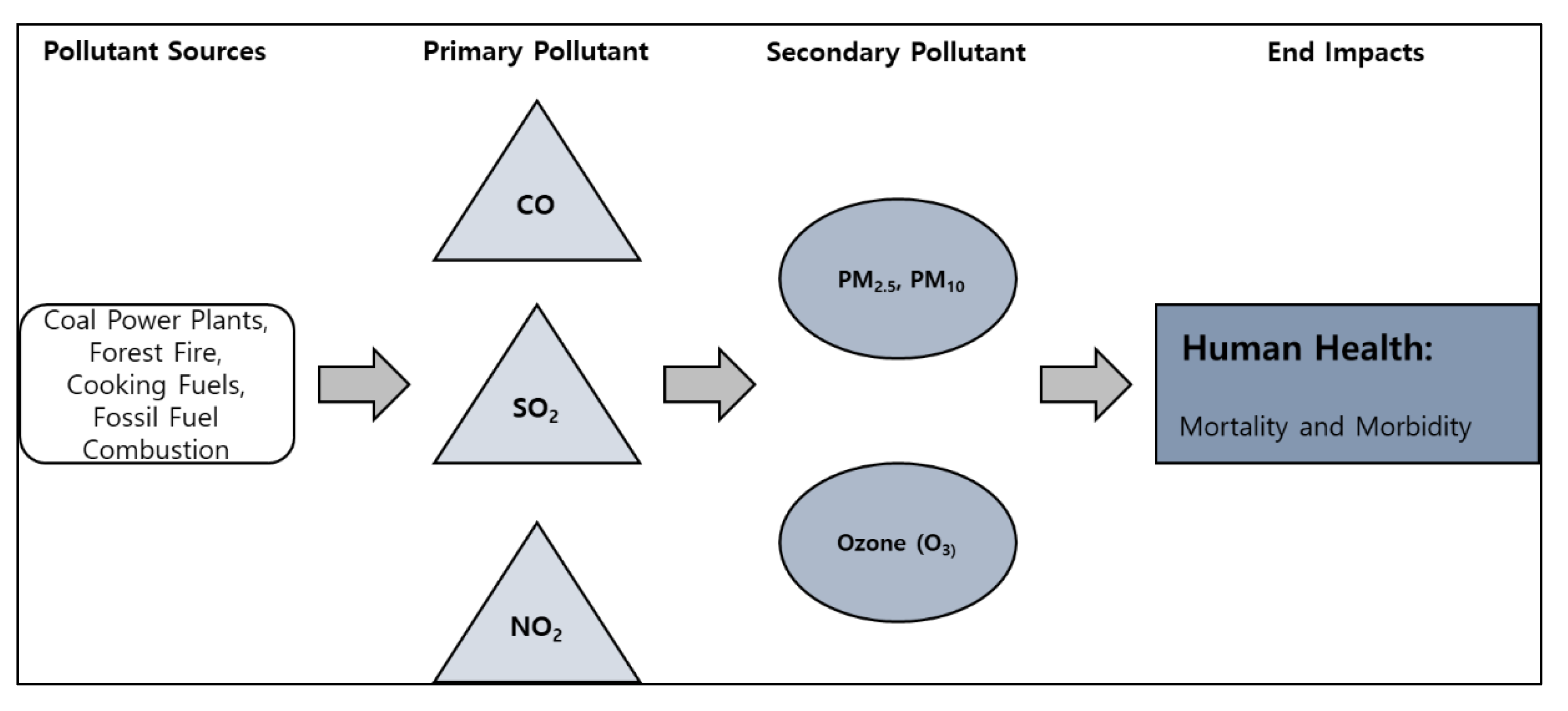
Increase in Air Pollutants and Asthma

Advancements in industry, urbanization, increased human activity due to population growth and the increased consumption of resources have led to the increase in air pollutants and consequent threats to human health. Air quality is being highlighted as a social issue and public interest and concern over respiratory health are increasing. Air pollutants can have chronic effects on the human body and pose a great risk because their effects are expressed in large population groups [1]. For example, London’s smog phenomenon in 1952 resulted in a total of 12,000 deaths due to atmospheric congestion and the surge in air pollutant concentrations, which raised public interest in the health hazards of air pollutants [2,3]. Air pollutants can generally cause the generation of pollutants in stages, as shown in Figure 1, due to the feedback action of various pollutants, resulting in complex reactions with the human body, which can lead to a variety of diseases compared to a single substance. Among them, the prevalence of respiratory diseases is assessed to be directly related to the effects of air pollutants [4,5,6,7,8,9]. Asthma, a representative respiratory disease that causes an increase in prevalence and socioeconomic burden worldwide, is thought to be associated with such an increase in air pollutants [10]. In addition to air pollutants, asthma deterioration can also be caused by allergens and occupational exposure, drugs, exercise, etc. Asthma is specifically known to be affected by particulate matter (PM), ozone (O3), nitrogen dioxide (NO2) and sulfur dioxide (SO2) among air pollutants [11,12,13,14].
The goal of this study is to predict asthmatic occurrence due to air pollution which could have a serious adverse effect on the human body, utilizing open big data released by the government. First, we verified variables that had been identified as significant to actual asthma according to related research. Second, we verified the causality and influence of the variables using the vector autoregressive model (VAR), which is primarily used for multivariate time-series analysis. Next, the constructed VAR model was mixed with a deep learning algorithm, which has emerged notably in recent years with the advent of the big data era, to construct a hybrid DNN optimized for the prediction of asthmatic occurrence. Finally, we verified the performance of the hybrid DNN algorithm and compared it with other time-series algorithms.

2. Related Research

2.1. Effects of Air Pollutants on Asthma

In general, air pollutants that can have a significant impact on the human body can be classified into gas-like substances, such as NO2, SO2, CO and O3, and particulate matter, such as PM10 and PM2.5. Gas-like substances affect changes in the composition of the atmosphere and are usually byproducts of human economic activities, such as the burning of fossil fuels. NO2, formed by nitrogen oxides, is considered one of the main sources of material that can cause air pollution. NO2 generated by burning fossil fuels is mainly generated from automobile exhaust, which tends to be present in high concentrations in urbanized and industrialized areas [15,16]. An increase in exposure to NO2 can increase respiratory tract hypersensitivity and it has become clear that it is a substance directly related to asthma prevalence, reducing the lung function of asthmatic patients [17,18,19,20]. SO2 is a substance caused mainly by the oxidation of sulfur contained in crude oil when refining or burning oil. Previous studies have shown that exposure to large amounts of SO2 can cause airway contraction and increase the prevalence of asthma through interaction with other air pollutants such as NO2 [21,22,23]. CO is a colorless and odorless gas generated by incomplete combustion of hydrocarbons. Automobile exhausts and combustion devices such as boilers and heaters are the main generators of CO. CO binds with hemoglobin in the blood inside the lungs and forms carboxy-hemoglobin (CoHb) which reduces oxygen-carrying capacity. Therefore, it can interfere with respiratory metabolism and have harmful effects on health [24,25,26,27]. O3 is produced by the photochemical oxidation of the sun’s rays between nitrogen oxides and hydrocarbons from automobile exhaust. O3 has the characteristic of increasing in concentration as temperature increases, which means its influence is stronger in summer [28]. High O3 concentration in the atmosphere can induce a decrease in lung function and an increase in airway hyper-sensitivity [29,30], and exposure in a high temperature environment in a short period of time, in particular, can induce worsening symptoms in asthmatic patients [31]. The problem of O3 outbreaks is expected to intensify in today’s society, where many abnormal temperatures occur, sometimes due to global warming. Lastly, particulate matter (PM), the worst by-product of industrialization which has been designated as a first-class carcinogen by the World Health Organization (WHO), is a substance composed by a mixture of solid and liquid particles. Particulate matter is called PM10 if the diameter of particle is less than 10µm and PM2.5 if the diameter is less than 2.5 µm. Particulate matter is mainly produced through combustion in industrial processes and chemical reactions with the primary pollutants generated by automobile exhaust. PM10 tends to be deposited in the upper airway or bronchus, and PM2.5 can have adverse effects on respiratory diseases such as in the small airway or alveoli, depending on the relative size of particles [32,33]. According to previous studies, exposure to high concentrations of particulate matter in a short period of time can worsen symptoms of asthma patients [34,35], and differences in the influence of particulate matter among age groups have been identified. Robert et al. analyzed the effect of PM2.5 on asthma for four groups (under 6, 6 to 18, 19 to 49, and over 50 years old); they confirmed that children and youth groups aged 6–18 are at the highest risk from particulate matter [30]. Ko et al. confirmed that the influence of particulate matter on asthma varies by age group, with the greatest impact between particulate matter and asthma in age groups under 14 years and the highest impact on acute deterioration in age groups 65 or older [36]. Overall, the influence of particulate matter on asthma is higher for the elderly and children than for adults.

2.2. Effects of Meteorological Changes on Asthma

Changes in temperature, humidity and air pressure can change the distribution of air pollutants and affect the concentration of allergens, such as pollen and mold spores in the atmosphere, leading to worsening symptoms in asthma patients. A study by Sutyajeet et al. confirmed the significance of asthma outbreaks for high temperatures and precipitation [37], and Renato et al. confirmed that climate change in certain areas can change the amount of pollen in the atmosphere, affecting allergic diseases such as asthma [38]. Antonio et al. analyzed the influence of climate on asthma and verified that a decrease in maximum air pressure and increase in humidity could have a significant impact on asthma [39]. Overall, meteorological change including climate change is a factor that interacts with the distribution of air pollutants and can have complex effects on asthma.

2.3. Prediction of the Asthmatic Occurrence

Asthma caused by the combined interaction of air quality and the meteorological environment, as described above, has increased in prevalence worldwide. This has caused a variety of socioeconomic problems. Katayoun et al. noted that the onset of asthma causes a burden on individuals and a decrease in productivity at the national level [40]. Patrick et al. proved that the frequency of hospitalization of asthmatic patients is 6.4 times higher than that of ordinary people, and emergency room visits are up to 1.8 times higher, which results in higher medical expenses and reduced productivity, which in turn increases the risk of unemployment [41]. Despite the increasing prevalence of asthma, which results in various social costs for the nation and individuals, most national disease management systems do not prioritize and manage asthma [42,43]. Therefore, most asthmatic patients visit emergency rooms or hospitals only if they have symptoms, due to cost problems and the absence of a national monitoring system. At a time when urbanization and industrialization are accelerating, the limitation is clear: most previous studies have focused on environmental policy suggestions about clinical case-based asthma, including factors which are not highly feasible at the moment.
We determined that greater efficiency can be achieved in the development of health policies and budget distribution at the national level and the training and deployment efficiency of emergency medical personnel in hospitals with the open innovation perspective if a clear number of patients could be predicted for the actual atmospheric environment [44,45]. The preceding studies confirmed that the impact of government policies can be interpreted through the VAR model used for multivariate time series data analysis [46,47], and in other studies there exist the cases which applied DNN models to predict the effectiveness of public health polices [48]. Based on these results, unlike previous studies that utilized clinical cases and cohort data, the focus of this study is on building a model that predicts the number of asthma patients in the future after deriving key factors that could cause asthma, based on long-term time series data in the atmospheric environment.

3. Materials and Methods

3.1. Datasets

This study utilized a total of 10 endogenous variables, including a total of 6 atmospheric data, 3 meteorological data and asthmatic occurrence data from Seoul, South Korea; the data from 2015 to 2017 were constructed as the train set and the data from 2018 were used as the test set to verify the performance of the prediction model.

3.1.1. Asthmatic Occurrence

The data, which were used as a prediction target in this study, included the number of asthma cases. They were extracted from the public portal [49] which provides open data based on the past cases managed by the Korean National Health Insurance Service. We used only the number of cases that occurred in Seoul, South Korea, from 2 January 2015 to 31 December 2018. In the case of weekends and holidays, the analysis was excluded to ensure the reliability of our analysis, as it is highly likely to be underestimated compared to the actual number of asthma patients due to hospitals being closed, etc. Information on the final data we utilized is shown in Table 1 and Figure 2.

3.1.2. Atmospheric Environments

The atmospheric data used in this study were extracted from Air Korea web sites [50], which is managed by the Korean Ministry of Environment. The data were daily-based and averaged across all monitoring stations located in Seoul, South Korea, from 2 January 2015 to 31 December 2018. Air Korea accumulates concentrations of air pollutants collected through 398 measurement networks in 112 cities and counties nationwide into the National Ambient Air Quality Monitoring Information System (NAMIS), and discloses most of the data to the public, so the reliability of the data for analysis is regarded as officially guaranteed. We excluded the data measured over weekends and holidays to enhance consistency with asthmatic occurrence data, and the collected data include SO2, CO, O3, NO2, PM10 and PM2.5. The data we finally used are shown in Table 2 and Figure 3.
As shown in Figure 3, there appears to be a major spike of PM10 in February 2015. This results from the combined effect of both yellow dust and air pressure in southern Mongolia and northern China at that time, and the previous study confirmed this to be suitable for actual observed data [51].

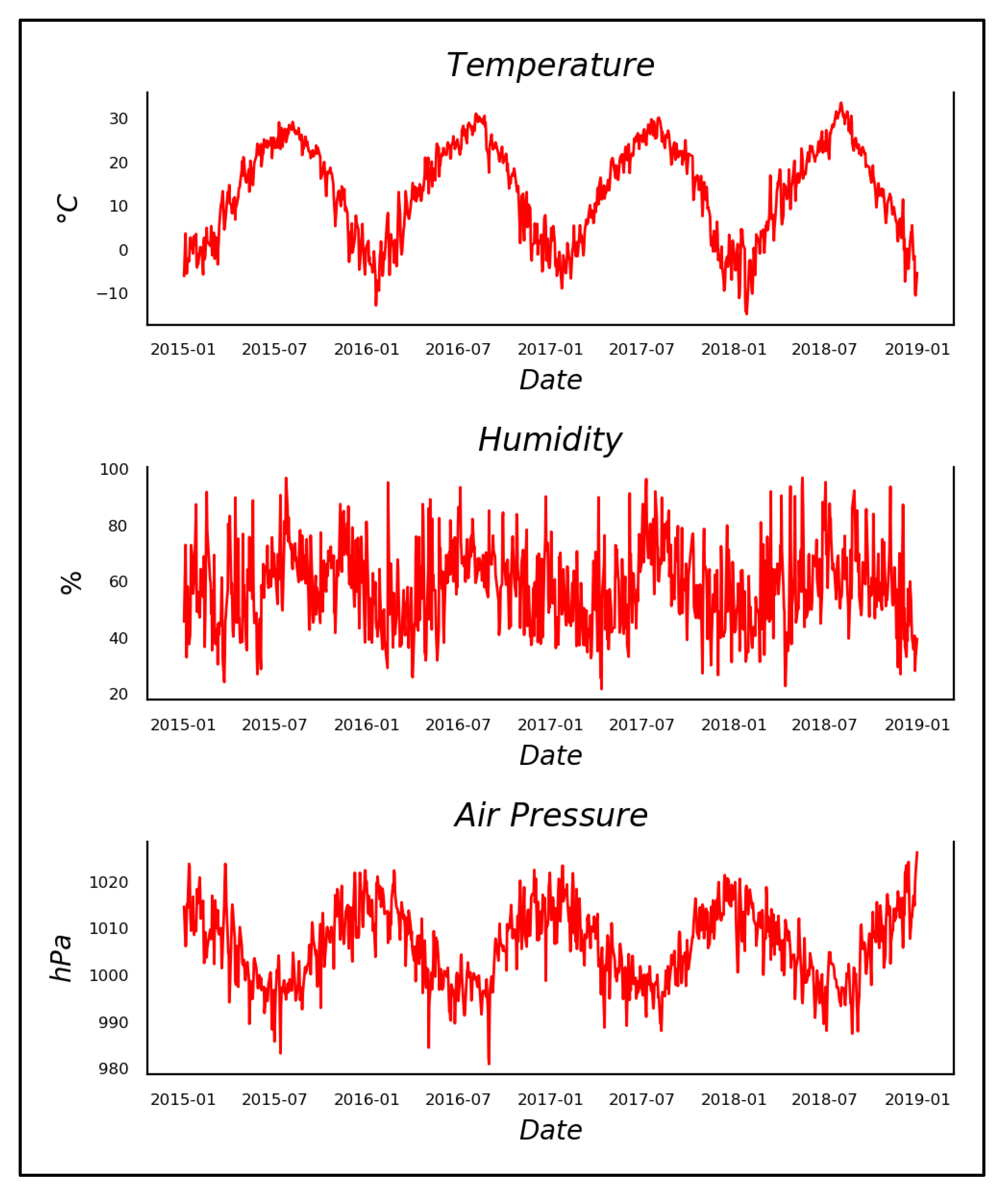
3.1.3. Meteorological Environments

The meteorological data used in this study were extracted from the Korea Meteorological Agency (KMA) web sites [52] based on the daily average at a monitoring station located in Seoul, South Korea, from 2 January 2015 to 31 December 2018. The KMA provides meteorological environment data obtained through the Automatic Synoptic Observation System (ASOS) as a public service, and the types and time differences of collectable data are also diverse, which is highly useful for analysis. Data from weekends and holidays were excluded to enhance consistency with the asthmatic occurrence data, and the finally utilized data are shown in Table 3 and Figure 4.

3.2. Methodology

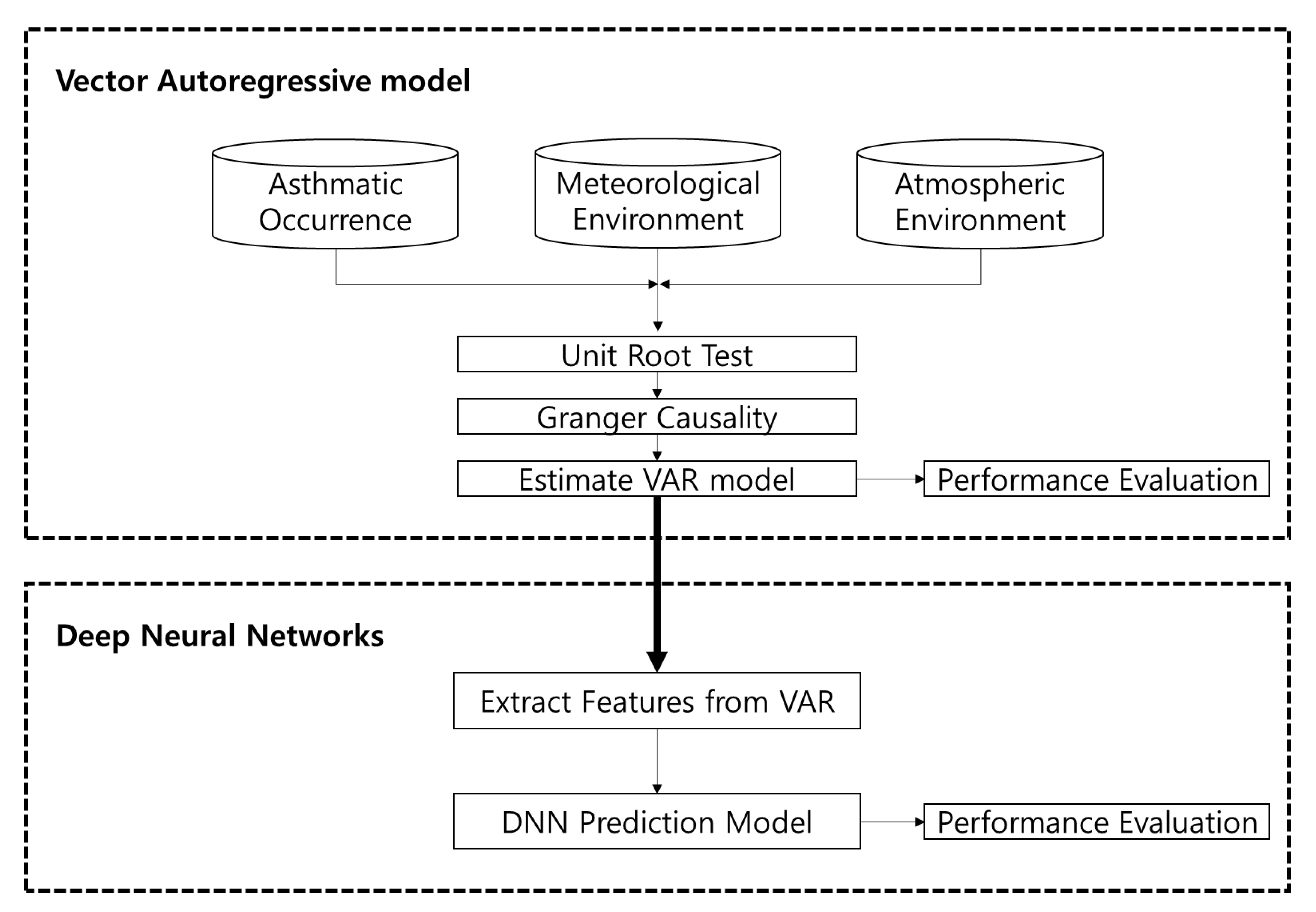
3.2.1. Vector Autoregressive Model

The vector autoregressive model (VAR), proposed by Sims [53], is represented in the form of a dynamic simultaneous equation in which the values for the past order of N variables with causality are used as endogenous variables to influence each other [54]. VAR (p) consists of an autoregressive process in which Xt = (X1t, X2t, X3t, ···, XNt) composed of N multivariate stationary time series is p time lags.
VAR (p) formula is as follows:
X t = C + θ 1 X t 1 + θ 2 X t 2 + + θ p X t p + ε t
X t = C + i = 1 p θ i X t i + ε t
( X 1 ,   t X 2 ,   t X 3 ,   t X N ,   t ) = ( C 1 C 2 C 3 C N ) + i = 1 P ( θ 11 θ 1 N θ N 1 θ N N ) i ( X 1 ,   t i X 2 ,   t i X 3 ,   t i X N ,   t i ) + ( ε 1 ,   t ε 2 ,   t ε 3 ,   t ε N ,   t )
where C means (N × 1) constant vector, θi means (N × N) matrix of the time difference regression coefficient between the current variable and the time difference variable, and εt means the white noise of (N × 1). In other words, X1,t is explained as its own past value and the past value of the other endogenous variable Xt, and the remainder that cannot be explained by the variable is explained by the white noise εt. Therefore, the multivariate stationary time series are compositely influenced by historical values from each other to interpret the current values [53].
The VAR model is applicable to stationary time series data. When non-stationary time series are used in the VAR model, the mean and covariance of the time series change over time and the exact model cannot be estimated. Therefore, before estimating the VAR model, it is necessary to conduct a unit root test to determine the stability of the time series. In this study, we applied the widely known augmented Dickey–Fuller (ADF) test to determine the stationary characteristics of each variable [55], and non-stationary time series data were converted to stationary time series through differences and then used to estimate the model.
The ADF formula is as follows:
Δ Y t = α + δ t + ρ t 1 + i = 1 p 1 γ i Δ Y t 1 + ε t
In general, the VAR model aims to reflect the composite influence between endogenous variables in the model. Therefore, the composition of the variables can be said to be significant in model estimation, among which the order of the variables is a meaningful symbolic factor in that the results in the impulse response function can be differently derived [56,57]. In this study, the Granger causality test, a type of VAR model, was used to construct the order of variables based on the precedence of variables.
The Granger causality formula is as follows:
X t = C + θ 1 X t 1 + θ 2 X t 2 + + θ p X t p + ε t
X t = C + θ 1 X t 1 + θ 2 X t 2 + + θ p X t p + ( θ 1 Y t 1 + θ 2 Y t 2 + + θ p Y t p ) + ε t
When the Granger causality test estimates the values of the stationary time series Xt, if it increases the significance of the model by using the value of the time lag p for Yt of Equation (6) in addition to the value of the time lag p for Xt of Equation (5), it is in general defined that Yt Granger cause Xt [56,57,58,59]. Thus, based on the results of Granger causality by endogenous variables, the order of the variables in VAR model can be determined by taking into account the order of the impact of each variable to the prediction target.
For the VAR model, unlike the utilization of the partial autocorrelation function (PACF) in the AR model, while we make use of the covariance matrix ∑p for the residuals of VAR model, the value p with minimal statistics for the following equations can be used as the time lag of the model. In this study, the equation for minimizing p is used as a model time lag determination criterion, considering the limitations of VAR models whose predictive performance decreases as the number of the variables to be estimated increases [60].
The criteria formula is as follows:
AIC ( Akaike   Information   Criteria ) :   ln | ^ p | + 2 k T p
BIC ( Bayesian   Information   Criteria ) :   ln | ^ p | + k ln ( T p ) T p
HQIC ( Hannan Qiunn   Information   Criteria ) :   ln | ^ p | + 2 k ln ( ln ( T p ) ) T p

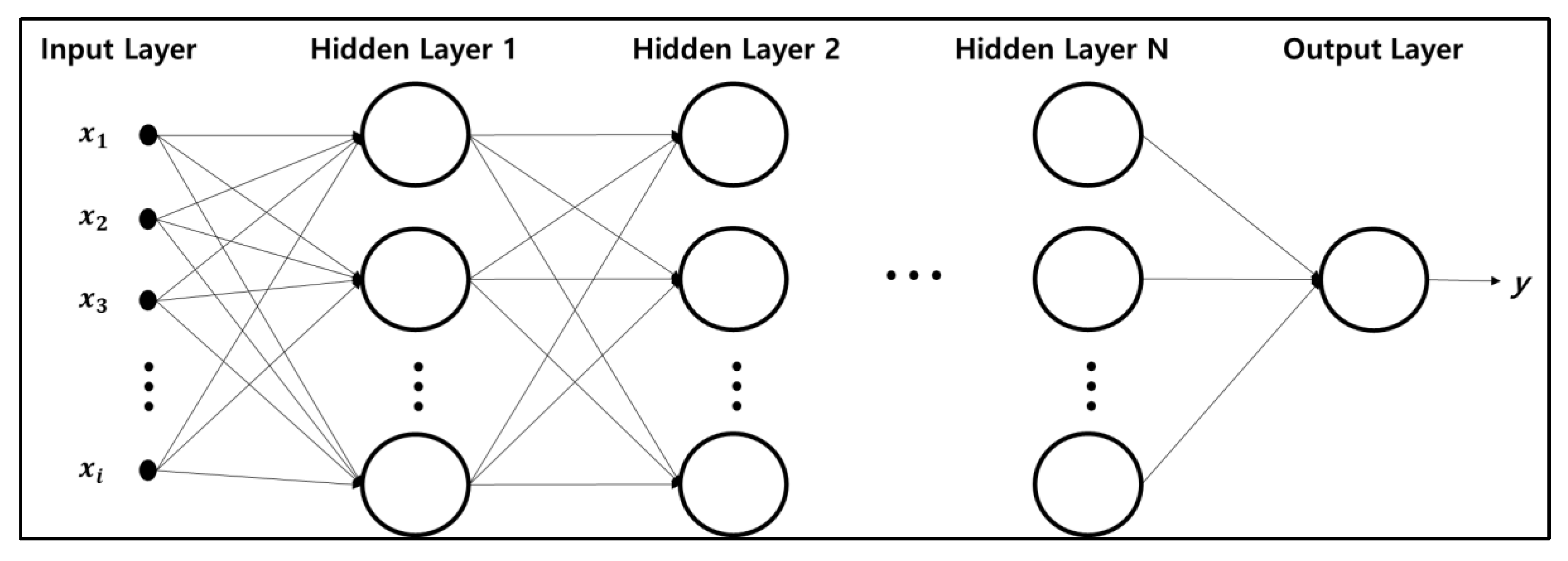
3.2.2. Hybrid Deep-Learning Model Based VAR & DNN

Deep neural networks (DNN) are one of the cutting-edge algorithms in this era of digital transformation. The usage and popularity of DNN have been rapidly increasing in recent years due to improvements in computing power and the ease of securing big data, and DNN has been regarded as a core player in future industries [61,62]. Unlike common linear models such as the linear regression (LR) model, DNN is evaluated as a model that takes into account nonlinearity, similar to real-world problems. DNN consists of an input layer to receive data input, multiple hidden layers and nodes, and an output layer to produce the final result (Figure 5). The nodes in each hidden layer are linked step by step to the output layer, and each node is filled with an intermediate calculation value from the input value to the output value. In this process, weight is assigned for each link, and each weighted sum (WS) is calculated for the associated node that it is applied to. The above process is for performing back-propagation to find the update value for the weight between each layer through gradient descent based on the error measured in the final output layer, and via a large number of iterations, ultimately to optimize the weight.
Since the weighted sum (WS) of each node is determined by sequential influence based on the x i utilized in the input layer for learning in DNN, the selection of variables to be used for learning has a strong influence on model performance [63].
The formula for the weighted sum is as follows:
W S = i = 1 n w i x i + ε
At a glance, the above formula seems similar to linear regression. Therefore, in this study, if the variable configuration of the estimated VAR model is structured by the DNN, the formula of the weighted sum of Equation (10) will be changed to the same form as the Equation (11) of the VAR, which will have a significant effect on improving the DNN prediction performance in a multivariate time series that includes the autoregressive (AR). In other words, the DNN model’s predictive performance can be enhanced by utilizing input variables with lag (p) estimated through the VAR model.
The weighted sum of the hybrid DNN formula is as follows:
W S o H = i = 0 n j = 1 p w i , t j x i , t j + ε ,         i f   x 0 = y
As a result, we propose to establish a hybrid deep learning model, with an open innovation perspective, comprehensively considering linearity and nonlinearity in multivariate time series using VAR and DNN in serial connection [64]. The model structure of the hybrid DNN model is shown in Figure 6.

4. Results

4.1. Vector Autoregressive Model

4.1.1. Unit Root Test

It is necessary to ensure that each endogenous variable consists of a stationary time series to establish assumptions for the correct estimation of the VAR model. Thus, in this study, the unit root test of the data was performed through the ADF test, and the first difference was performed to ensure that the time series data were stationary if the null hypothesis was not rejected at the 5% significance level. The results are shown in Table 4.
As a result of the ADF test, it was confirmed that O3 (atmospheric parameter), temperature and air pressure (meteorological parameter) were non-stationary time series at a 5% significance level. Those variables can also be observed as being non-stationary in Figure 3 and Figure 4, and to mitigate the non-stationary characteristics and to convert them into stationary time series, we utilized the first difference under the ADF test. From the results of the first difference, as shown in Table 4, we confirmed that all variables are stationary data. Finally, we were able to use stationary time series data to construct the model.

4.1.2. Granger Causality

The estimation of the VAR model can be aimed at reflecting the composite influence between variables in the model, so it is necessary to ensure that each variable has a sequential influence on the asthmatic occurrence and determine whether it is a variable that can have causality in the actual asthmatic occurrence. In this study, through the aforementioned Granger causality test, we tried to derive the logical order of variables to be used in the model. Table 5 shows the results of the Granger causality test for endogenous variables in this model.
The results of the Granger causality test indicate that Granger causality exists in the asthmatic occurrence for all variables except O3. In the case of O3, there is no direct Granger causality for asthmatic occurrence, but it was confirmed that Granger causality exists for endogenous variables such as SO2 and CO that affect asthmatic occurrence. Therefore, it is appropriate to include O3 as an endogenous variable in the model, as it is judged to affect asthmatic occurrence through sequential interaction with other variables. Based on the results of the test, we identified a number of variables that constitute feedback or bilateral causality, which may be interpreted as indicating the possibility that other exogenous variables were involved in the causality between the two variables. This means that it is necessary to utilize some additional exogenous variables in addition to the constructed variables. Finally, the order of variable composition of the VAR model estimated based on the causal results and degree of erogeneity of the Granger causality test was AiPr, O3, Temp, PM2.5, CO, PM10, Hum, NO2, SO2 and AsO. In addition, the dummy variable (Hol) immediately before and after the expected date of a holiday or weekend and seasonal dummy variables (Su, Au, Wi) were added to take into account the seasonality and yearly trend of the endogenous variables to be used in estimating the VAR model [65,66].

4.1.3. Estimation of VAR Model

The results of AIC, BIC and HQIC were used to select the optimal time-lag p of the VAR model by utilizing 10 endogenous variables and 4 dummy variables, as shown in Table 6.
There were differences in the results: BIC derived 1 from the model’s optimal time-lag, but AIC judged the model’s optimal time-lag as 6 and HQIC as 3. Because including too many variables in the model could cause problems in estimating the model due to the reduction in the degree of freedom, this study estimated VAR (1) for asthmatic occurrence based on the BIC.
The formula of VAR (1) for asthmatic occurrence is as follows:
X A s O , t = C + δ 1 H o l + δ 2 S u + δ 3 A u + δ 4 W i + θ 1 X A i P r , t 1 + θ 2 X O 3 , t 1 + θ 3 X T e m p , t 1   + θ 4 X P M 2.5 , t 1 + θ 5 X C O , t 1 + θ 6 X P M 10 , t 1 + θ 7 X H u m , t 1 + θ 8 X N O 2 , t 1   + θ 9 X S O 2 , t 1 + θ 10 X A s O , t 1 + ε t
Table 7 shows the estimated VAR (1) results for the asthmatic occurrence to be used in this study among the estimated VAR (1) models.
As a result of the p-value in VAR (1), the occurrence of asthma can be interpreted as being significantly affected by the asthmatic occurrence of the day before, holiday, temperature, NO2 and SO2. In addition, throughout the results of the variance inflation factor (VIF), which are typically used to check for the multi-collinearity of the variables, we confirmed that all variables in the model do not have multi-collinearity because their values are below the value of 10 [67,68,69].
Figure 7 is the result of the impulse response of endogenous variables to asthmatic occurrence. First, when 1hPa impulse was applied to the air pressure, the asthmatic occurrence showed an increase of about 9.25 after 1 day, and it was confirmed that the influence converges to zero after 5 days. O3 causes an increase of about 2575.59 a day after the impulse of 1ppm and 3423.64 two days later, with its influence rapidly decreasing thereafter. Temperature can cause a decrease in asthmatic occurrence of about 54.15 when an impulse of 1 °C is applied, and its influence has been confirmed to converge at zero after about 7 days. This result is slightly different from the findings of the preceding study [37], and as shown in Figure 2 and Figure 4, the actual asthmatic occurrence can be interpreted as having relatively little influence on the frequency of visits due to the concentration of allergens at high temperatures. PM2.5 shows that an impulse of 1 µg/m3 can cause a decrease of 54.15 in asthmatic occurrence after one day, and it has been confirmed that the influence converges at zero after about seven days, which does not appear to be highly credible when checking the p-value and confidence interval of Figure 7 in the model. It was confirmed that CO could cause an increase of about 292.69 in asthmatic occurrence a day later when 1 ppm of impulse was applied, and its influence could last for a relatively long period. PM10 causes a decrease of approximately 0.99 in asthmatic occurrence after one day when an impulse of 1 µg/m3 is applied, and its influence immediately converges to zero. In addition to PM2.5, the confidence interval and p-value are considered unreliable. Humidity increases the asthmatic occurrence by about 3.47 after one day if an impulse of 1% is applied, and the influence converges to zero after about three days, reaffirming that the influence of the allergen concentration on asthmatic occurrence is not significant, as in the case of temperature. It was confirmed that the impulse of NO2 1 ppm could increase the asthmatic occurrence by about 12,622.22, and that its influence could continue after two weeks. Finally, in the case of SO2, it was confirmed that when an impulse of 1 ppm was applied, the asthmatic occurrence could increase by about 95,442.85 after one day, and its influence could continue for a rather long period of time, just as in the case of SO2.
To sum up the results, some variables did not have high significance in p-value, resulting in a mixture of positive (+) and negative (−) in the confidence interval for the impulse response. It is believed that logical interpretation will be possible based on empirical judgment and previous research. In addition, the fact that these interpretations of the meteorological environment are somewhat different from previous studies seems to reflect the discriminatory characteristics of this study using large, generalized data, unlike small clinical data, and this is considered to be noteworthy. Given that the effects of the impulse response are longer along the order of the variables, it is confirmed that the correct variable configuration was successful, taking advantage of the results of Granger causality.
Finally, Figure 8 shows the result of verifying the predicted performance of the finally estimated VAR (1) for asthmatic occurrence using the test set as the goal of this study.
The estimated model seems to reflect the flow and pattern of increases and decreases in general, but due to the limitations of the OLS-based linear model, it was confirmed that some predictions were limited, such as the surge in patients in abnormal situations that reflected nonlinear patterns.

4.2. Hybrid Deep Neural Networks

4.2.1. Extract Features from VAR Model

The type of variable used in the estimation of previous VAR (1) is composed of yt-1 and xt-1 for the predicted value yt (XAsO, t) and the dummy variables as in Equation (12). In the hybrid DNN model utilized in this study, the above variables were used as the input variable in the same form, and the ultimate form of the model is shown in Figure 9.
The designed model was made to reflect the complicated pattern of variables by including 128 nodes for each of the three hidden layers and set the hyper-parameter to have a 0.001 learning rate and 300 epochs. At this time, in order to prevent the over-fitting of the model for the train set, drop out was specified to exclude some nodes for each hidden layer during learning, and judging that the raw data’s time series characteristics were reflected in a single line, the learning was conducted through random sampling, which excludes consideration of the time series by line. In addition, the model’s optimization was performed using the Adam optimizer. Mean absolute error (MAE) was used for the loss function.

4.2.2. Performance Evaluation of Hybrid DNN

The results of verification using the test set for the proposed hybrid DNN model are shown in Figure 10 and Figure 11.
The model confirmed that the loss graph was reduced due to smooth learning, and the predictive performance of the random sampling test set was also significant. The mean absolute error (MAE) for the model’s asthmatic occurrence is approximately 479, indicating an error of about 8.17% compared to the daily average of about 5860.
To validate the performance of this hybrid DNN, its predictive performance was compared with those of other algorithms by utilizing the same data. Table 8 shows the results of performance measurements and comparisons of general DNN, VAR models and long short-term memory (LSTM), which are known to have high predictive performance for existing time series data.
The results for each performance evaluation confirm that hybrid DNN demonstrated the best performance, deduced to be the result of the combination of linearity of VAR and nonlinearity of DNN.

5. Conclusions

Air quality and favorable surrounding environment in daily life are so crucial for human beings’ sustainable life. Nevertheless, the problems of air pollution continue to intensify, due to increased human activity directly relevant to the advancement of industry. Although respiratory diseases such as asthma are high-risk candidates that can be immediately affected by these problems, most countries do not place priority on the disease management of asthma. This study proposes a prediction model to predict asthmatic occurrence by utilizing the deep neural network algorithm, which enhanced usability in model analysis for existing problem resolving, utilizing the advancement of computing power and the potentials of big-data collection. The proposed hybrid model of VAR and DNN, referred to as the hybrid DNN model, has the advantage of being able to simultaneously reflect both linear and nonlinear patterns for data in the stage of learning the model. In addition, the proposed model is also meaningful in that VAR can help overcome some of the DNN’s limitations which made it impossible to interpret that the effects of variables in the existing model. The influence on asthmatic occurrence was confirmed by the impulse response of VAR, confirming that seasonality, temperature and SO2 influences in the model were the greatest. Variables that were considered to have a significant impact on asthma, such as particulate matter, based on previous clinical case-based studies, were found not to have significance for asthmatic occurrence. In addition, the finding of this study that lower temperature, as in winter, could adversely affect asthma is incompatible with previous studies. This is the evidence that the pattern in the data, showing that the number of asthma patients increases in winter, as shown in Figure 2, has been appropriately reflected in the model. Unlike previous studies, this approach is meaningful in that it can identify asthmatic occurrence patterns in relation to the atmospheric and meteorological environment and also identify the general impact of each variable on disease using the result of impulse response in VAR. In fact, atmospheric and meteorological factors in the real world have interrelations and can be viewed as an interaction variable that functions like an integrated single variable. Therefore, we utilized the VAR model and ADF test that could identify the optimal time lag, which is determined from either the minimum value of Akaike information criterion (AIC) or Schwartz information criterion (SIC), where each variable has a concurrent effect on asthmatic occurrence in order to enhance the possibility of interrelations among variables in the real world and the predicted performance of the hybrid model. Finally, the performance of the proposed model has been compared with other time series forecasting models, confirming that the mean absolute error (MAE) demonstrated the best performance at about 8.17%, underscoring that this model was highly applicable.
Unlike preceding studies conducted in limited samples such as clinical and cohort data for conventional asthma patients, this study presented a new directionality for atmospheric and meteorological data-driven disease research in that constantly updated, large-scale open data for the prediction modeling and analysis are credibly collected at the national level. In addition, it could also be also extensively applied by appropriately changing the parameters of the model suitable for any specific countries in which the data could be obtained. The features of this hybrid deep learning algorithm can provide the possibility of sustainable research expansion from the perspective of creative open innovation [70].
In summary, it is believed that predictions of future asthmatic occurrence through our proposed hybrid deep-learning model with open innovation perspective will improve efficiency in the management and resource allocation of national health insurance and budgets, and also guarantee efficiency in the deployment of medical personnel in hospitals [70]. In addition, through the selection of criteria for the number of predicted patients and the development of asthma risk indexes, early notification systems based on the atmospheric environment for chronic patients will contribute to the increase in national health and socioeconomic productivity. It is also expected that the proposed model will be highly applicable to all engaged in disease analysis in general, as it can be used to predict the number of patients with other diseases, and the prediction range can be expanded to all disease groups such that the data-and-model-based alarming could provide a good solution toward coping with current sustainability and open innovation perspective [71].

Author Contributions

Conceptualization, M.-S.K. and T.-E.S.; Data curation, J.-H.L.; Formal analysis, J.-H.L., Y.-J.J., C.-H.L. and J.-H.C.; Methodology, M.-S.K. and Y.-J.J.; Writing–original draft, M.-S.K. and J.-H.L.; Writing–review & editing, T.-E.S. All authors have read and agreed to the published version of the manuscript.

Funding

This research received no external funding.

Acknowledgments

The authors would like to thank the Editor and the anonymous reviewers for their thoughtful and constructive comments that have greatly improved this manuscript.

Conflicts of Interest

The authors declare no conflict of interest.

References

  1. Kwon, H.J.; Cho, S.H.; Kim, M.S.; Ha, M.N.; Han, S.W. Cross-sectional Study on Respiratory Symptoms due to Air Pollution Using a Questionnaire. Korea J. Prev. Med. 1994, 27, 313–325. [Google Scholar]
  2. Lee, H.J.; Kim, Y.W.; Lee, H.S.; Jang, Y.J. A Cluster Analysis on the Risk of Particulate Matter Focusing on Differences of Risk-Related Behaviors based on Public Segmentation. J. Public Relat. Res. 2016, 20, 201–235. [Google Scholar]
  3. Bert, B.; Stephen, T.H. Air Pollution and Health. The Lancet 2002, 360, 1233–1242. [Google Scholar]
  4. Nino, K.; Ira, B.T. Air Pollution: From Lung to Heart. Swiss Med. Wkly. 2005, 135, 697–702. [Google Scholar]
  5. Pope, C.A., III; Richard, T.B.; Michael, J.B.; Eugenia, E.C.; Daniel, K.; Kazuhiko, I.; George, D.T. Lung Cancer, Cardiopulmonary Mortality, and Long-term Exposure to Fine Particulate Air Pollution. J. Am. Med. Assoc. 2002, 287, 1132–1141. [Google Scholar]
  6. Andrew, J.G.; Robert, B.D. Inflammatory Lung Injury after Bronchial Instillation of Air Pollution Particles. Am. J. of Respir. Crit. Care Med. 2001, 164, 704–708. [Google Scholar]
  7. Boris, Z.S.; Michael, T.K.; Robert, A.K. Air Pollution and Cardiovascular Injury. J. Am. Coll. Cardiol. 2008, 52, 719–726. [Google Scholar]
  8. Fredrik, N.; Per, G.; Lars, J.; Tom, B.; Niklas, B.; Robert, J.; Goran, P. Urban Air Pollution and Lung Cancer in Stockholm. Epidemiology 2000, 11, 487–495. [Google Scholar] [CrossRef]
  9. Laura, P.; Christophe, D.; Carmen, I.; Inmaculada, A.; Chiara, B.; Ferran, B.; Catherine, B.; Olivier, C.; Francisco, B.C.; Francesco, F.; et al. Chronic Burden of Near-roadway Traffic Pollution in 10 European Cities (APHEKOM network). Eur. Respir. J. 2013, 42, 594–605. [Google Scholar]
  10. Park, D.W.; Kim, S.H.; Yoon, H.J. The Impact of Indoor Air Pollution on Asthma. Allergy Asthma Respir. Dis. 2017, 5, 312–319. [Google Scholar] [CrossRef] [Green Version]
  11. Choi, K.U.; Paek, D.M. Asthma and Air Pollution in Korea. Korean J. Epidemiol. 1995, 17, 64–75. [Google Scholar]
  12. Kim, S.H.; Son, J.Y.; Lee, J.T.; Kim, T.B.; Park, H.W.; Lee, J.H.; Kim, T.H.; Son, J.W.; Shin, D.H.; Park, S.S.; et al. Effect of Air Pollution on Acute Exacerbation of Adult Asthma in Seoul, Korea: A Case-crossover Study. Korean J. Med. 2010, 78, 450–456. [Google Scholar]
  13. Michael, G.; John, R.B. Outdoor Air Pollution and Asthma. Lancet 2014, 383, 1587–1592. [Google Scholar]
  14. Piotr, O.C.; Piotr, D.; Aneta, O.J.; Michalina, B.; Ernest, C.; Tomasz, O.; Patrycja, R.K.; Artur, B. A Preliminary Attempt at the Identification and Financial Estimation of the Native Health Effects of Urban and Industrial Air Pollution Based on the Agglomeration of Gdaǹsk. Sustainability 2020, 12, 42. [Google Scholar]
  15. Esther, R.; Nicole, A.H.J.; Patricia, H.N.V.; Bert, B. Personal and Outdoor Nitrogen Dioxide Concentration in Relation to Degree of Urbanization and Traffic Density. J. Am. Coll. Cardiol. 2008, 52, 719–726. [Google Scholar]
  16. Andreas, R.; John, P.B.; Hendrik, N.; Claire, G.; Ulrike, N. Increase in Tropospheric Nitrogen Dioxide over China Observed from Space. Nature 2005, 437, 129–132. [Google Scholar]
  17. Hong, S.J.; Seo, J.H. Climate Change and Human Health. J. Korean Med. Assoc. 2011, 54, 149–155. [Google Scholar] [CrossRef]
  18. KIM, M.K. The Survey of Nitrogen Dioxide in Indoor Environment. J. Korean Soc. Environ. Anal. 2010, 13, 161–165. [Google Scholar]
  19. Jane, Q.K. Air Pollution and Asthma. J. Allergy Clin. Immunol. 1999, 104, 717–722. [Google Scholar]
  20. Yutong, C.; Wilma, L.Z.; Dany, D.; Marta, B.; Paul, R.B.; Isabel, F.; Amadou, G.; Kees, D.H.; Kristian, H.; Stephane, M.; et al. Ambient Air Pollution, Traffic Noise and Adult Asthma Prevalence: A BioSHaRE Approach. European Respir. J. 2017, 49, 1502127. [Google Scholar]
  21. Jang, A.S. Climate Change and Air Pollution. J. Korean Med. Assoc. 2011, 54, 175–180. [Google Scholar] [CrossRef]
  22. Chin, Y.J.; Park, N.G.; Lee, H.S.; Kim, D.S.; Eom, J.H.; Cho, M.C.; Yoon, S.J.; Jeong, H.S.; Song, H.G.; Sung, R.H.; et al. The Inflammatory Response in Mouse Lung after Acute Sulfur Dioxide Exposure. Tuberc. Respir. Dis. 1994, 41, 328–338. [Google Scholar]
  23. Henry, G., Jr.; William, S.L.; Sheryl, L.T.; Karen, R.A.; Kenneth, W.C. Anti-inflammatory and Lung Function Effects of Montelukast in Asthmatic Volunteers Exposed to Sulfur Dioxide. CHEST 2001, 119, 402–408. [Google Scholar]
  24. Harrison, R.M.; Thornton, C.A.; Lawrence, R.G.; Mark, D.; Kinnersley, R.P.; Ayres, J.R. Personal Exposure Monitoring of Particulate Matter, Nitrogen Dioxide and Carbon Monoxide, Including Susceptible Groups. Occupat. Environ. Med. 2002, 59, 671–679. [Google Scholar] [CrossRef] [PubMed]
  25. Kristin, A.E.; Jill, S.H.; Philip, K.H.; Maria, F.; David, Q.R. Increased Ultrafine Particles and Carbon Monoxide Concentrations are Associated with Asthma Exacerbation among Urban Children. Environ. Res. 2014, 129, 11–19. [Google Scholar]
  26. Im, H.J.; LEE, S.Y.; Yun, K.J.; Ju, Y.S.; Kang, D.H.; Cho, S.H. A Case-crossover Study between Air Pollution and Hospital Emergency Room Visits by Asthma Attack. Korean J. Occupat. Environ. Med. 2000, 12, 249–257. [Google Scholar] [CrossRef]
  27. Yasuda, H.; Yamaya, M.; Yanai, M.; Ohrui, T.; Sasaki, H. Increased Blood Carboxyhaemoglobin Concentrations in Inflammatory Pulmonary Diseases. Thorax 2002, 57, 779–783. [Google Scholar] [CrossRef] [Green Version]
  28. Bryan, J.B.; Jeffrey, W.S.; Charles, A.P.; Ross, J.S.; Russell, R.D. Observed Relationships of Ozone Air Pollution with Temperature and Emissions. Geophys. Res. Lett. 2009, 36, L09803. [Google Scholar]
  29. Matthew, J.S.; Lyndsey, A.D.; Mitchel, K.; Dana, W.F.; Jeremy, A.S.; Lance, A.W.; Stefanie, E.S.; James, A.M.; Paige, E.T. Short-term Associations between Ambient Air Pollutants and Pediatric Asthma Emergency Department Visits. Am. J. Respir. Crit. Care Med. 2010, 182, 307–316. [Google Scholar]
  30. Robert, A.S.; Kazuhiko, I. Age-related Association of Fine Particles and Ozone with Severe Acute Asthma in New York City. J. Allergy Clin. Immunol. 2010, 125, 367–373. [Google Scholar]
  31. Ke, Z.; Xiaobin, L.; Liuhua, S.; Ge, T.; Cristine, T.L.; Sabine, L.; Julie, E.G. Concentration-response of Short-term Ozone Exposure and Hospital Admissions for Asthma in Texas. Environ. Int. 2017, 104, 139–145. [Google Scholar]
  32. Gehui, W.; Liming, H.; Shixiang, G.; Songting, G.; Liansheng, W. Measurements of PM10 and PM2.5 in Urban Area of Nanjing, China and the Assessment of Pulmonary Deposition of Particle Mass. Chemosphere 2002, 48, 689–695. [Google Scholar]
  33. Hao, Y.; Linyu, X. Comparative Study of PM10/PM2.5—Bound PAHs in Downtown Beijing, China: Concentrations, Sources and Health Risk. J. Clean. Product. 2018, 177, 674–683. [Google Scholar]
  34. Christian, S.; Nino, K.; Jean, P.B.; Philippe, L.; Werner, K.; Regula, R.; Christian, M.; Ursula, A.L. Short-Term Variation in Air Pollution and in Average Lung-Function Among Never-Smokers. Am. J. Respir. Crit. Care Med. 1999, 163, 356–361. [Google Scholar]
  35. Jennifer, K.M.; John, R.B.; Tim, A.B.; Kathleen, M.M.; Helene, G.M.; Boriana, P.; Katharine, H.; Frederick, W.L.; Ira, B.T. Short-Term Effects of Air Pollution on Wheeze in Asthmatic Children in Fresno, California. Environ. Health Perspect. 2010, 118, 1497–1502. [Google Scholar]
  36. Ko, F.W.S.; Tam, W.; Wong, T.W.; Lai, C.K.W.; Wong, G.W.K.; Leung, T.F.; Ng, S.S.S.; Hui, D.S.C. Effects of Air Pollution on Asthma Hospitalization Rates in Different =Age Groups in Hong Kong. Clin. Exp. Allergy 2007, 37, 1312–1319. [Google Scholar] [CrossRef] [PubMed]
  37. Sutyajeet, S.; Chengsheng, J.; Jared, F.; Crystal, R.U.; Clifford, M.; Amir, S. Exposure to Extreme Heat and Precipitation Events Associated with Increased Risk of Hospitalization for Asthma in Maryland, USA. Environ. Health 2016, 15. [Google Scholar] [CrossRef] [Green Version]
  38. Renato, A.; Giorgio, W.C.; Giovanni, P. Possible Role of Climate Changes in Variations in Pollen Seasons and Allergic Sensitizations during 27 Years. Ann. Allergy Asthma Immunol. 2010, 104, 215–222. [Google Scholar]
  39. Antonio, C.; Jane, F.; Emil, K.; Rory, J.S. Thunderstorm Associated Asthma: A Detailed Analysis of Environmental Factors. Br. Med. J. 1996, 312, 604–607. [Google Scholar]
  40. Katayoun, B.; Mary, M.D.W.; Carlo, M.; Larry, L.; Kadria, A.; John, S.; Mark, F. Economic Burden of Asthma: A Systematic Review. BMC Pulm. Med. 2009, 9, 24. [Google Scholar]
  41. Patrick, W.S.; Julia, F.S.; Vahram, H.G.; Brandon, S.; Denise, R.G.; Lin, S.L.; Gary, G. The Relationship between Asthma, Asthma Control and Economic Outcomes in the United States. J. Asthma 2014, 51, 769–778. [Google Scholar]
  42. Bousquet, J.; Dahl, R.; Khaltaev, N. Global Alliance against Chronic Respiratory Diseases. Eur. Respir. Soc. 2007, 29, 233–239. [Google Scholar] [CrossRef] [PubMed]
  43. Matthew, M.; Denise, F.; Shaun, H.; Richard, B. The Global Burden of Asthma: Executive Summary of GINA Dissemination Committee Report. Allergy 2004, 59, 469–478. [Google Scholar]
  44. Biancone, P.; Secinaro, S.; Brescia, V.; Calandra, D. Management of Open Innovation in Healthcare for Cost Accounting Using EHR. J. Open Innov. Technol. Mark. Complex. 2019, 5, 99. [Google Scholar] [CrossRef] [Green Version]
  45. Yun, J.J.; Zhao, X.; Jung, K.; Yigitcanlar, T. The Culture for Open Innovation Dynamics. Sustainability 2020, 12, 5076. [Google Scholar] [CrossRef]
  46. Carlos, V.S. Monetary Policy and the US Housing Market: A VAR Analysis Imposing Sign Restrictions. J. Macroecon. 2008, 30, 977–990. [Google Scholar]
  47. Horng, M.S.; Chang, Y.W.; Wu, T.Y. Does Insurance Demand or Financial Development Pomote Economic Growth? Evidence from Taiwan. Appl. Econ. Lett. 2012, 19, 105–111. [Google Scholar] [CrossRef]
  48. Xing, H.L.; Hiroshi, M.; Joseph, V.; Yu, M.; David, L.B. Guiding Public Health Policy by Using Grocery Transaction Data to Predict Demand for Unhealthy Beverage. Stud. Comput. Intell. 2020, 843, 169–176. [Google Scholar]
  49. Public Data Portal. Available online: https://www.data.go.kr/data/15028050/fileData.do (accessed on 1 April 2020).
  50. Air Korea. Available online: http://www.airkorea.or.kr (accessed on 1 April 2020).
  51. Park, M.E.; Cho, J.H.; Kim, S.; Lee, S.S.; Kim, J.J.; Lee, H.C.; Cha, J.W.; Ryoo, S.B. Case Study of the Heavy Asian Dust Observed in Late February 2015. Atmosphere 2016, 26, 257–275. [Google Scholar] [CrossRef] [Green Version]
  52. Korea Meteorological Agency. Available online: http://data.kma.go.kr (accessed on 1 April 2020).
  53. Sims, C.A. Macroeconomics and Reality. Econometrica 1980, 48, 1–48. [Google Scholar] [CrossRef] [Green Version]
  54. Yoon, J.S.; Huh, N.K.; Kim, S.; Hur, H.Y. A Study on International Passenger and Freight Forecasting Using the Seasonal Multivariate Time Series Models. Commun. Appl. Methods 2010, 17, 473–481. [Google Scholar] [CrossRef]
  55. Sutthichaimethee, P.; Chatchorfa, A.; Suyaprom, S. A Forecasting Model for Economic Growth and CO2 Emission Based on Industry 4.0 Political Policy under the Government Power: Adapting a Second-Order Autoregressive-SEM. J. Open Innov. Technol. Mark. Complex. 2019, 5, 69. [Google Scholar] [CrossRef] [Green Version]
  56. Chun, H.J. An Empirical Analysis on the Relationship between Economic Growth and Income Inequality. Seoul Stud. 2014, 15, 95–111. [Google Scholar]
  57. Kim, C.H.; Nam, J.O. A Causality Analysis of the Hairtail Price by Distribution Channel Using a Vertor Autoregressive Model. J. Fish. Bus. Adm. 2015, 46, 93–107. [Google Scholar]
  58. Lee, Y.H.; Kim, H.K. Financial Support and University Performance in Korean Universities: A Panel Data Approach. Sustainability 2019, 11, 5871. [Google Scholar] [CrossRef] [Green Version]
  59. Li, H.; Li, B.; Lu, H. Carbon Dioxide Emissions, Economic Growth, and Selected Types of Fossil Energy Consumption in China: Empirical Evidence from 1965 to 2015. Sustainability 2017, 9, 697. [Google Scholar]
  60. Park, H.J.; Park, C. A Study on the Prospective in Korean Land Market Using Vector Auto-Regressive Model. Korean Spat. Plan. Rev. 2001, 31, 1–13. [Google Scholar]
  61. Méndez-Suárez, M.; García-Fernández, F.; Gallardo, F. Artificial Intelligence Modelling Framework for Financial Automated Advising in the Copper Market. J. Open Innov. Technol. Mark. Complex. 2019, 5, 81. [Google Scholar] [CrossRef] [Green Version]
  62. Lee, J.; Suh, T.; Roy, D.; Baucus, M. Emerging Technology and Business Model Innovation: The Case of Artificial Intelligence. J. Open Innov. Technol. Mark. Complex. 2019, 5, 44. [Google Scholar] [CrossRef] [Green Version]
  63. Tereq, H.; Siby, J.P.; Radha, K.A.; Prakash, R.; Hossein, S. Short-term Load Forecasting Using Deep Neural Networks(DNN). In Proceedings of the IEEE 2017 North American Power Symposium, Morgantown, WV, USA, 17–19 September 2017; pp. 1–6. [Google Scholar]
  64. Yun, J.J.; Kim, D.; Yan, M.-R. Open Innovation Engineering-Preliminary Study on New Entrance of Technology to Market. Electronics 2020, 9, 791. [Google Scholar] [CrossRef]
  65. Mo, S.J. Demand Pattern of the Global Passengers: Sea and Air Transport. J. Korea Port Econ. Assoc. 2011, 27, 1–11. [Google Scholar]
  66. Karoliina, P.S.; Piia, A.; Markku, O.; Heikki, T. Climate Change and Electricity Consumption-witnessing Increasing or Decreasing Use and Costs? Energy Policy 2010, 38, 2409–2419. [Google Scholar]
  67. José, D.C.; José, C.P. The Corrected VIF (CVIF). J. Appl. Stat. 2011, 38, 1499–1507. [Google Scholar]
  68. Wujung, V.A.; Mbella, M.E. Entrepreneurship and Poverty Reduction in Cameroon: A Vector Autoregressive Approach. Arch. Bus. Res. 2014, 2, 1–11. [Google Scholar] [CrossRef]
  69. Alibuhtto, M.C. Modelling Colombo Consumer Price Index: A Vector Autoregressive Approach. J. Manag. 2014, 11, 74–81. [Google Scholar]
  70. Yun, J.J.; Lee, D.; Ahn, H.; Park, K.; Yigitcanlar, T. Not Deep Learning but Autonomous Learning of Open Innovation for Sustainable Artificial Intelligence. Sustainability 2016, 8, 797. [Google Scholar] [CrossRef] [Green Version]
  71. Krajcsák, Z. Implementing Open Innovation Using Quality Management System: The Role of Organizational Commitment and Customer Loyalty. J. Open Innov. Technol. Mark. Complex. 2019, 5, 90. [Google Scholar] [CrossRef] [Green Version]
Figure 1. Summary of pollutant steps.
Sustainability 12 06143 g001
Figure 2. Daily asthmatic occurrence data.
Sustainability 12 06143 g002
Figure 3. Daily atmospheric data.
Sustainability 12 06143 g003
Figure 4. Daily meteorological data.
Sustainability 12 06143 g004
Figure 5. Structure of the deep neural networks.
Sustainability 12 06143 g005
Figure 6. Structure of the proposed hybrid deep learning model.
Sustainability 12 06143 g006
Figure 7. Result of impulse responses in VAR (1).
Sustainability 12 06143 g007
Figure 8. Result of forecasting asthmatic occurrence using VAR (1).
Sustainability 12 06143 g008
Figure 9. Final structure of the hybrid deep neural network (DNN).
Sustainability 12 06143 g009
Figure 10. Loss graph of the hybrid DNN.
Sustainability 12 06143 g010
Figure 11. Result of forecasting asthmatic occurrence using the hybrid DNN.
Sustainability 12 06143 g011
Table 1. Summary statistics for asthmatic occurrence data.
VariablesMeanMedianKurtosisSkewnessPercentiles
Min25th75thMax
Occurrence5859.595737.000.170.562699.004728.006724.0011,881.00
Table 2. Summary statistics for atmospheric data.
VariablesMeanMedianKurtosisSkewnessPercentiles
Min25th75thMax
SO2 (ppm)0.0050.0053.3211.2160.0030.0040.0060.013
CO (ppm)0.5640.5201.3881.2170.2800.4430.6361.251
O3 (ppm)0.0200.020−0.3770.3740.0030.0120.0270.053
NO2 (ppm)0.0370.0360.0840.5470.0140.0280.0450.082
PM10 (1 µg/m3)46.76343.393122.8457.1507.97531.76857.227555.692
PM2.5 (1 µg/m3)24.34822.1542.2491.2293.27515.37330.37887.821
Table 3. Summary statistics for meteorological data.
VariablesMeanMedianKurtosisSkewnessPercentiles
Min25th75thMax
Temperature (°C)13.2814.40−1.06−0.2714.803.5023.1033.70
Humidity (%)58.5458.60−0.360.1521.8047.6068.1097.00
Air Pressure (hPa)1006.091006.70−0.66−0.07981.0999.601012.501026.20
Table 4. t-statistics of augmented Dickey–Fuller (ADF) unit root test.
VariablesAt the LevelFirst Difference
t-Statisticsp-Valuet-Statisticsp-Value
Asthmatic OccurrenceAsO−2.89650.0457 **−2.89650.0457 **
Atmospheric EnvironmentSO2−4.54970.0001 ***−4.54970.0001 ***
CO−4.00740.0013 **−4.00740.0013 **
O3−2.74080.0672 *−11.6995<0.0001 ***
NO2−8.5039<0.0001 ***−8.5039<0.0001 ***
PM10−5.4865<0.0001 ***−5.4865<0.0001 ***
PM2.5−8.7544<0.0001 ***−8.7544<0.0001 ***
Meteorological EnvironmentTemp−2.29990.1719−4.34130.0003 ***
Hum−4.24810.0005 ***−4.24810.0005 ***
AiPr−2.09030.2484−12.9901<0.0001 ***
1 AsO interpreted as asthmatic occurrence, Temp interpreted as temperature, Hum interpreted as humidity and AiPr interpreted as air pressure.; 2 *, ** and *** stand for 10%, 5% and 1% levels of significance, respectively.
Table 5. p-value of the Granger causality test.
Dependent VariablesAsOSO2COO3NO2PM10PM2.5TempHumAiPr
AsO1.00 <0.01 ***<0.01 ***0.21<0.01 ***0.03 **<0.01 ***<0.01 ***<0.01 ***0.05 **
SO2<0.01 ***1.00<0.01 ***0.08 *<0.01 ***0.14<0.01 ***<0.01 ***<0.01 ***<0.01 ***
CO<0.01 ***0.231.000.05 **<0.01 ***0.10 *<0.01 ***<0.01 ***<0.01 ***<0.01 ***
O30.350.07 *<0.01 ***1.00<0.01 ***0.720.15<0.01 ***<0.01 ***<0.01 ***
NO2<0.01 ***<0.01 ***0.06 *<0.01 ***1.000.07 *0.19<0.01 ***<0.01 ***<0.01 ***
PM10<0.01 ***<0.01 ***<0.01 ***0.40<0.01 ***1.00<0.01 ***<0.01 ***<0.01 ***0.36
PM2.50.01 ***<0.01 ***<0.01 ***0.03 **<0.01 ***0.04 **1.00<0.01 ***<0.01 ***<0.01 ***
Temp0.06 *<0.01 **<0.01 ***<0.01 ***<0.01 ***0.17<0.01 ***1.000.03 **<0.01 ***
Hum<0.01 ***<0.01 ***<0.01 ***<0.01 ***<0.01 ***<0.01 ***<0.01 ***<0.01 ***1.00<0.01 ***
AiPr0.40<0.01 ***<0.01 ***<0.01 ***<0.01 **0.04 **0.02 **<0.01 ***<0.01 ***1.00
1 *, ** and *** stand for 10%, 5% and 1% levels of significance, respectively; 2 maximum lag of model is limited to two weeks.
Table 6. Results of Information Criteria.
LagAICBICHQIC
0−5.454−5.140−5.333
1−8.327−7.386 *−7.964
2−8.582−7.014−7.977 *
3−8.726−6.531−7.879
4−8.828−6.006−7.740
5−9.136−5.686−7.805
6−9.219 *−5.142−7.646
7−9.137−4.434−7.323
8−9.026−3.695−6.970
9−8.952−2.994−6.654
10−8.869−2.284−6.329
1 * stand for minimum value of each information criterion; 2 maximum lag of the model is limited to two weeks.
Table 7. Result of vector autoregressive model (VAR) (1) for asthmatic occurrence.
VariablesCoefficientt-Statisticsp-ValueVIF
C 2138.3436.425<0.001 ***
H o l −1717.08826.210<0.001 ***1.190
S u −1359.116−11.449<0.001 ***2.528
A u −275.489−2.5710.010 **1.980
W i 174.5051.4490.1472.560
X A i P r , t 1 9.2451.2040.2291.153
X O 3 ,   t 1 2575.5870.5580.5771.171
X T e m p , t 1 −54.148−4.059<0.001 ***1.317
X P M 2.5 ,   t 1 −4.435−0.8490.3964.271
X C O , t 1 292.6890.5510.5817.890
X P M 10 ,   t 1 −0.995−0.5680.5702.645
X H u m ,   t 1 3.4721.1910.2341.666
X N O 2 ,   t 1 12,668.2251.8650.062 *5.915
X S O 2 ,   t 1 95,442.8512.0620.039 **2.670
X A s O ,   t 1 0.38314.864<0.001 ***2.090
1 *, ** and *** stand for 10%, 5% and 1% levels of significance, respectively.
Table 8. Performance evaluation of the models.
ModelLearning RateEpochPerformance Evaluation
MAEMSERMSEMAPE
Hybrid DNN0.001300479.31473,295.40687.968.20
VAR668.5071,750.20847.2013.17
DNN0.001300691.22818,571.94904.7511.87
LSTM0.001100821.721140,624.001068.0015.01

