A Multi-Objective Model for Sustainable Perishable Food Distribution Considering the Impact of Temperature on Vehicle Emissions and Product Shelf Life

Abstract

The food distribution process is responsible for significant quality loss in perishable products. However, preserving quality is costly and consumes a tremendous amount of energy. To tackle the challenge of minimizing transportation costs and CO₂ emissions while also maximizing product freshness, a novel multi-objective model is proposed. The model integrates a vehicle routing problem with temperature, shelf life, and energy consumption prediction models, thereby enhancing its accuracy. Non-dominated sorting genetic algorithm II is adapted to solve the proposed model for the set of Solomon test data. The conflicting nature of these objectives and the sensitivity of the model to shelf life and shipping container temperature settings are analyzed. The results show that optimizing freshness objective degrade the cost and the emission objectives, and the distribution of perishable foods are sensible to the shelf life of the perishable foods and temperature settings inside the container.

1. Introduction

Improving the sustainability of a distribution network involves tradeoffs between multiple conflicting objectives, including minimizing transportation costs (e.g., fuel and vehicle maintenance costs, driver salaries), fulfilling customer requirements (e.g., on-time deliveries, short lead times), and limiting environmental impact (e.g., vehicle emissions). However, optimizing sustainability in perishable food distribution is particularly challenging, primarily because of temperature control requirements [1]. Temperature is a major determinant of the shelf life of a perishable product [2,3,4]. Even small or infrequent deviations from recommended temperature settings can significantly reduce product shelf life [5,6,7] because increased temperature accelerates the growth rate of the microorganisms that are responsible for quality degradation in perishable foods [5,8]. Although refrigerated vehicles’ cargo is well-isolated, it can experience frequent exposure to increased temperature when the vehicle stops to make deliveries to other customers [2,9]. As a result, an estimated 8–23% loss in perishable food quality occurs during the distribution process [10].

This loss in quality increases the likelihood that the food is wasted [11]. According to the United States Department of Agriculture, 30–40% of food in the U.S. is wasted [12], with 40% of these losses occurring post-harvest [13]. As a result, much of the resources consumed by the production and distribution of perishable food, as well as their associated environmental impacts, are in vain [13]. It is estimated that food waste costs the U.S. economy $218 billion each year [14]. Moreover, as described by Mercier et al. [11], quality loss due to inadequate temperature control increases food safety risk. In the U.S., the annual societal costs of foodborne illness are estimated to be $50 billion [15], with more than 120,000 hospitalizations and 3000 fatalities annually [16]. Therefore, it is crucial to maintain the predefined temperature range for perishable food products during distribution to ensure their quality and safety [17,18,19,20].

A distribution plan that emphasizes short transit times and few stops can preserve product quality and reduce waste. However, the energy required to transport and refrigerate perishable products during distribution is supplied by burning fossil fuels, which releases greenhouse gases into the environment [17]. In fact, food refrigeration during transportation accounts for 15% of global fossil fuel consumption and 40% of the global greenhouse effect [18], with up to 40% of refrigerated vehicles’ emissions generated by a conventional diesel engine vapor compression refrigeration system [21]. In terms of cost and energy, delivering multiple orders using a single full truck is more efficient than delivering each individual order on its own dedicated route. However, a full truckload increases order transit times, as well as the frequency of temperature abuses during unloading, thereby reducing product quality and increasing food waste.

Consolidated logistics and distribution is a suitable solution for integrated food supply chain networks where preserving the quality of perishable products and reducing distribution costs and CO₂ emissions are common sustainable goals for upstream food supply chain actors, such as farmers, food manufacturers, and distribution centers, food distributors, such as third party logistics companies, and downstream supply chain actors, such as supermarkets, restaurants, and grocery stores. As an example, a group of supermarkets can consolidate their orders from one supplier in a horizontally integrated supply chain where food suppliers, food distributors, and supermarkets benefit from preserving the quality of perishable items and lowering distribution costs and CO₂ emissions in the distribution process. Thus, attempts to simultaneously maximize product freshness while minimizing vehicle emissions and transportation costs in a perishable food distribution network involve tradeoffs. These tradeoffs indicate the necessity of incorporating multiple objectives when studying the problem of perishable food distribution. For example, some studies consider both product perishability and distribution costs (e.g., Wang et al. [22] and Rahbari et al. [23]). The tradeoff between emissions and distribution costs has also been analyzed (see e.g., Xiao et al. [24]). However, few studies integrate distribution costs, freshness, and CO₂ emissions simultaneously, and the precision of existing studies has been limited by simplifying assumptions (e.g., Musavi & Bozorgi-Amiri [25]). The integrated approaches can assess and optimize the effect of routing decisions on the sustainability goals of food supply chain actors.

The research presented in this paper introduces a novel extension of the multi-objective vehicle routing problem for the sustainable distribution of perishable food products. In this multi-objective sustainable vehicle routing problem (MO-SVRP), products are dispatched from a depot and are delivered to a set of customers having deterministic demand. Temperature is the primary controllable element in preserving the quality of perishable food products. To capture this, the MO-SVRP model is extended by integrating a method for predicting heat exchange and temperature inside the shipping container, thereby allowing product freshness and vehicle energy consumption to be accurately estimated. This integrated model considers three objectives: maximization of average product freshness, minimization of total CO₂ emissions, and minimization of total distribution costs. The MO-SVRP is solved using a non-dominated sorting genetic algorithm (NSGA-II), which provides schedules and routes for the efficient distribution of perishable products using refrigerated vehicles.

The paper is organized as follows: Section 2 presents a review of the related literature. Section 3 provides the problem statement and model formulation. Section 4 shows the solution procedure. In Section 5, computational results and a discussion of the findings are presented. Finally, the conclusion of this research and recommendations for future research are provided in Section 6.

2. Literature Review

There is a rich literature related to the distribution of perishable food. The review presented in this paper focuses on literature that uses mathematical modeling to optimize food distribution systems.

Transit time and temperature are the two most influential factors on the quality of delivered perishable food products. Integrating product transit time is straightforward for mathematical models that are already tracking delivery times for other purposes, such as time window constraints. Therefore, many studies that take perishability into account consider the reduction of transit time directly or indirectly in their models [10,26,27,28,29,30,31]. These models assume that the rate of product deterioration is constant over time, such that minimizing product time in transit is linearly equivalent to an increase in the quality of the delivered products [32]. Hence, transit time is used as a proxy for product quality loss, either as part of cost minimization or revenue maximization objective.

However, the inherent tradeoffs between delivering high-quality products and minimizing distribution costs have inspired researchers to consider them as separate objectives. The multi-objective model developed by Bortolini et al. [32] minimizes delivery time as a separate objective to represent the freshness of delivered foods. Similarly, Amorim and Almada-Lobo [33] Musavi and Bozorgi-Amiri [25], and Rahbari et al. [23] used a multi-objective approach to study product freshness maximization, where freshness was linearly estimated. Amorim, Günther, & Almada-Lobo [34] and Hsu, Chen, and Wu [35] integrated the effect of temperature into the rate of quality degradation, such that the rate of quality degradation increases with increasing storage temperature. Since the growth rate of microorganisms that spoil food is exponential, the impact of temperature variations on product shelf life can be estimated using exponential functions, which can then be maximized [22,36,37,38].

Temperature-controlled transportation is energy-intensive and consequently releases a large volume of CO₂ emissions into the environment. The energy required to carry a load between two locations is evaluated in Bektaş & Laporte’s [39] study with respect to traveled distance, vehicle acceleration speed, the slope of the road, the weight of the load, the density of air, and the frontal surface of the vehicle. Stellingwerf et al. [17] adapted this methodology to evaluate CO₂ emissions for both transportation and refrigeration, based on the assumption of constant energy losses during unloading and through the walls of the vehicle. Wang et al. [38] transformed CO₂ emissions and the energy required for transportation and refrigeration into costs, which were minimized. Accorsi, Gallo, & Manzini [40] calculated the energy consumption of distribution activities, which were then minimized in the objective function. Hsu et al. [31] integrated the effects of energy required for refrigeration of perishable products as a part of a cost minimization objective, where the cost of energy is a function of the constant and predetermined temperature inside the container, ambient temperature, volume of the container, duration of each stop, and frequency of opening the container. Hsu et al. [35] optimized the delivery of perishable products having different temperature requirements, accounting for refrigeration costs as a component of distribution costs. Some studies include CO₂ emissions in a separate objective of a multi-objective model (see e.g., Bortolini et al. [32], Govindan, Jafarian, Khodaverdi, & Devika [41], Molina, Eguia, Racero, & Guerrero [42], Musavi & Bozorgi-Amiri [25], and Wang et al. [43]), allowing decision-makers to assess the impact of reducing CO₂ emissions on other food distribution system objectives, as well as the marginal cost of reducing environmental effects.

Most models in the literature seek to maximize product quality throughout the distribution process. By contrast, Devapriya et al. [44], Khalili-Damghani et al. [45] and Nakandala, Lau, & Zhang [46] added a set of constraints to their model to ensure that the quality of the delivered products meets customers’ expectations. Hsu et al. [31] calculated the volume of spoiled products based on the duration and ambient temperature of each delivery stop. Novaes et al. [9] used commercial software to predict the temperature inside the shipping container, using time-temperature data to evaluate the quality of products at each delivery location via a statistical indicator in a traveling salesman problem.

The impact of sustainability goals was reflected in multi-objective models. Several studies addressed the environmental and economic effects of the food supply chain in bi-objective models (see e.g., Govindan et al. [41], Soysal et al. [47], and Validi et al. [48]). The quality and safety of perishable products are affected by storage and distribution process time and temperature. Hence, Accorsi, Baruffaldi, and Manzini [49] evaluated the impact of temperature on operation efficiency and the safety of perishable products in a bi-objective study. Bortolini et al. [32] added the delivery time minimization as the third objective to the environmental and economic objectives to reduce the effect of traveling time on losing the quality of perishable products.

A diverse set of solution strategies have been used to solve the perishable food distribution problem. Ghezavati et al. [27] adapted a Benders decomposition model to solve a mixed-integer linear program. Chen et al. [26] and Farahani et al. [30] adapted a heuristic algorithm to solve the distribution planning problem as part of their production and distribution model. Metaheuristic approaches have also been widely used to find good-quality solutions in a reasonable amount of time. These approaches are also useful for finding a Pareto optimal frontier in multi-objective problems. Musavi and Bozorgi-Amiri [25] applied NSGA-II on a multi-objective hub location scheduling problem, in which total transportation costs and carbon emissions were minimized and food freshness was maximized. Amorim and Almada-Lobo [33] applied $\epsilon$-constraint method to a small-scale problem and NSGA-II to a large-scale multi-objective problem that aimed to minimize total routing costs and maximize average freshness in a food distribution problem. Khalili-Damghani et al. [45] solved a bi-objective location-routing problem for the distribution of perishable products using the $\epsilon$-constraint and NSGA-II algorithm. Their result showed that the NSGA-II solutions were as good as the $\epsilon$-constraint solutions, but the metaheuristic algorithm outperformed the exact method in terms of solving time, especially for larger-scale problems. Govindan et al. [41] used a hybrid approach that integrated an adapted multi-objective particle swarm optimization (MOPSO) and an adapted multi-objective variable neighborhood search (AMOVNS) to solve a bi-objective location routing problem for perishable products with economic and environmental minimization objectives.

A summary of the important features of the related literature is given in

Table 1. A comparison of the important features of the related literature.

Literature	Quality Degradation Changes				Method of Addressing Perishability	Objectives			Temperature Effect on Quality	Emission		Temperature Effect on Emissions	Temperature Prediction	Solution Method
	Linear over Time	Linear over Temperature	Nonlinear over Time	Nonlinear over Temperature		Economic	Perishability	Emissions		Transportation	Refrigeration			Exact	Heuristic	Metaheuristic
Hsu et al. [31]	x				The predicted amount of spoiled products are added to the shipment to ensure orders are filled	x			x		x	x			x
Osvald & Stirn [10]	x				Minimize delivery time	x									x
Chen et al. [26]	x				Minimize product deterioration, assuming a constant rate	x									x
Wang et al. [43]					Does not address perishability	x		x		x				x
Ahumada & Villalobos [29]	x				Minimize product decay	x								x
Farahani et al. [30]	x				Minimize time between production and delivery	x									x
Amorim et al. [34]	x	x			Maximize fractional remaining shelf life	x	x							x
Hsu et al. [35]					Does not address perishability	x					x					x
Govindan et al. [41]					Does not address perishability	x		x		x						x
Molina et al. [42]					Does not address perishability	x		x		x					x
Amorim & Almada-Lobo [33]	x				Maximize average freshness	x	x							x		x
Khalili-Damghani et al. [45]	x				Constrain delivery of products to occur before they expire	x								x		x
Bortolini et al. [32]	x				Minimize delivery time	x	x	x		x				x
Wang et al. [22]			x	x	Maximize freshness	x	x								x
Ghezavati et al. [27]	x				Minimize quality degradation and disposal costs	x								x
Devapriya et al. [44]	x				Constrain delivery of products to occur before they expire	x									x
Hsiao et al. [36]			x	x	Minimize loss in shelf life as product-related costs	x										x
Gallo et al. [37]			x	x	Minimize energy consumed to cool down products spoiled in transportation			x		x	x			x
Musavi & Bozorgi-Amiri [25]	x				Maximize purchase probability	x	x	x		x						x
Albrecht & Steinrücke [28]	x				Maximize revenue from the grade of quality	x								x
Wang et al. [38]			x		Minimize product damage costs in the objective function	x				x	x					x
Stellingwerf et al. [17]					Does not address perishability	x		x		x	x			x
Rahbari et al. [23]	x				Maximize freshness	x	x							x
This research			x	x	Maximize average freshness	x	x	x	x	x	x	x	x			x

. The related literature is ordered from oldest to the newest, and “x” represents that the publication included the specific feature in their study. Most of these studies either focus on food product perishability or the environmental impacts of temperature-controlled distribution. Only two studies cover cost, freshness, and emissions, and only Hsu et al. [31] and Novaes et al. [9] have considered the effect of temperature on product quality and carbon emissions.

To the best of our knowledge, the multi-objective vehicle routing problem (VRP) model presented in this paper is the first to use an integrated temperature prediction method to estimate product quality and refrigeration energy consumption while accounting for cost, freshness, and emissions in a perishable food distribution system. Specifically, this paper extends the MO-SVRP by adding a heat exchange model to accurately estimate the temperature inside the refrigerated container. This allows for a more accurate prediction of product freshness (i.e., shelf life) upon delivery, as well as improving the estimation of total emissions generated by refrigerated trucks. This paper also utilizes a novel adaptation of the NSGA-II metaheuristics algorithm to solve the MO-SVRP model.

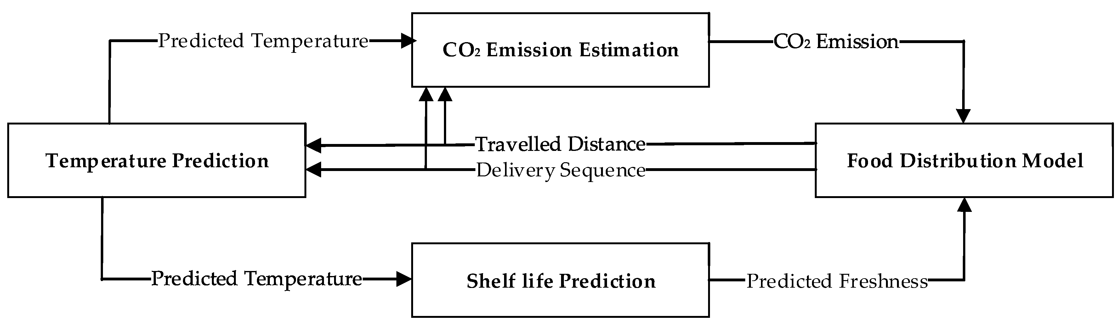
3. Problem Statement and Model Formulation

Distribution problems typically seek to consolidate the flow of goods from a depot to their demand destinations into fewer routes [50]. The vehicle routing problem (VRP) is often utilized to formulate this problem, such that an optimal (i.e., minimum distance) route is determined, subject to constraints such as route connectivity, vehicle capacity limits, and the number of available vehicles. The model described in this paper integrates a VRP with methods that accurately predict temperature, estimate CO₂ emissions, and predict product freshness.

The proposed MO-SVRP model consists of the interconnected perishable food distribution modules including distribution model, temperature prediction, CO₂ emission, and shelf life prediction. The distribution model provides vehicles’ delivery sequence and traveled distance which then are used to predict temperature inside the vehicle. The predicted temperatures are the key element of estimating the shelf life of the foods at their destination. The predicted temperature along with routing information enables the CO₂ estimation module to predict the environmental effect for the proposed routing plan. The predicted freshness of perishable products, CO₂ emission estimates, and distribution costs are the sustainability objectives of the MO-SVRP model. Figure 1 presents the integrated structure of the MO-SVRP model. In the remainder of this section, each of these methods and their mathematical relations are presented, and then the MO-SVRP assumptions, notations, and model are illustrated.

3.1. Temperature Prediction Based on Heat Transfer

The cooling unit in a refrigerated vehicle is constantly trying to preserve the temperature inside the container by blowing cold air. However, each time the vehicle makes a delivery stop and opens the container door for unloading, the heat exchange between the hot ambient air and cold container air raises the temperature inside the container. The capacity of the cooling equipment and the amount of heat exchange are the main factors that determine the temperature inside the container. In the MO-SVRP model, energy balance equations are applied to predict the temperature inside the container.

Since heat exchange when the vehicle is in transit differs from unloading, the container temperature in each of these stages is predicted using different methods. When the vehicle is moving, the cooling system runs until the temperature inside the container reaches the desired level (Td), and a thermostat turns the cooling system off. In most cases, the vehicle’s cooling system and engine are turned off during unloading to protect the engine and to avoid polluting the air around the delivery dock. Therefore, it is assumed that the cooling system is not running during unloading, and therefore the temperature inside the container can only increase.

3.1.1. Temperature Prediction during Unloading

According to the energy balance equation, the overall heat that enters the container is equal to the accumulated heat inside the container (Equations (1)–(2); Holdsworth et al. [51]). The heat entering and accumulating inside the container at customer location j are denoted by AE_j and AH_j, respectively.

$$A{E}_j=m_a.r_o.s_a.\left(T_j-T_0\right).t$$

(1)

$m_a$: Air mass (kg)

$r_a$: Air transfer ratio

$s_a$: Specific heat of the air (J kg⁻¹ K⁻¹)

$T_j$: The ambient temperature at location j (K)

$T_0$: Current temperature inside the container (K)

$t$: Portion of unloading time ($t\le u_j$)

$$A{H}_j=\left(m_j{s}_c+m_a{s}_a\right)\frac{dT}{dt}$$

(2)

$m_j$: Cargo mass at location j (kg)

$m_a$: Air mass (kg)

$s_c$: Specific heat of cargo (J kg⁻¹ K⁻¹)

$s_a$: Specific heat of the air (J kg⁻¹ K⁻¹)

$\frac{dT}{dt}$: Rate of change in temperature (K)

Following the energy balance equation, the temperature at customer j, given an unloading time t, can be estimated using Equation (3). Detailed derivation of Equation (3) is presented in Appendix A.

$$T_j=T_a-\left(T_a-T_0\right).e^{-\frac{m_a.r_o.s_a}{\left(m_j{s}_c+m_a{s}_a\right)}.t}$$

(3)

$m_j$: Cargo mass at location j (kg)

$m_a$: Air mass (kg)

$s_c$: Specific heat of cargo (J kg⁻¹ K⁻¹)

$s_a$: Specific heat of the air (J kg⁻¹ K⁻¹)

$\frac{dT}{dt}$: Rate of change in temperature (K)

3.1.2. Temperature Prediction during Transportation

When the engine is running, the cooling equipment begins to remove the heat absorbed during the unloading process until the container temperature reaches Td. The rate of heat removal is denoted by Q_c:

$$Q_C=\left(m_{ij}{s}_c+m_a{s}_a\right)\frac{dT}{dt}$$

(4)

$m_{ij}$: Cargo mass between location i and j (kg)

$m_a$: Air mass (kg)

$s_c$: Specific heat of cargo (J kg⁻¹ K⁻¹)

$s_a$: Specific heat of the air (J kg⁻¹ K⁻¹)

$\frac{dT}{dt}$: Rate of change in temperature (K H⁻¹)

Applying the energy balance enables the prediction of container temperature during transportation between locations i and j (T_ij) using Equation (5). Detailed derivation of Equation (5) is presented in Appendix A.

$$T_{ij}=\frac{Q_c}{\left(m_{ij}{s}_c+m_a{s}_a\right)}.t+T_0$$

(5)

$Q_c$: The capacity of cooling equipment (J H⁻¹)

$m_{ij}$: Cargo mass between location i and j (kg)

$m_a$: Air mass (kg)

$s_c$: Specific heat of cargo (J kg⁻¹ K⁻¹)

$s_a$: Specific heat of the air (J kg⁻¹ K⁻¹)

$t$: Time duration (h)

$T_0$: Current temperature inside the container (K)

Equation (5) shows that the cooling equipment reduces the temperature at a rate of $\frac{Q_c}{\left(m_{ij}{s}_c+m_a{s}_a\right)}$. However, since the cooling equipment stops blowing cold air when the temperature reaches Td, the actual temperature is as follows:

$$T_{ij}^{\ast }=Max\left\{T_{ij},T_d\right\}$$

(6)

3.2. CO₂ Emissions

The main source of CO₂ emissions in a perishable food distribution system is the fuel that is burned to provide energy for transport and refrigeration. The energy required for transportation, which is not specific to perishable products, depends primarily on the distance traveled, the weight of the vehicle and its cargo, the vehicle speed, and road/vehicle specifications. Bektaş & Laporte [39] developed a widely used method that integrates all these factors to predict road transportation energy consumption:

$$p_{ij}\approx {\alpha }_{ij}\left(w+f_{ij}\right)d_{ij}+\beta v_{ij}^2{d}_{ij}$$

(7)

$w$: Vehicle weight

$f_{ij}$: Weight of the load between node i to j

$v_{ij}$: Vehicle velocity

$d_{ij}$: Distance between nodes i and j

${\alpha }_{ij}$: Arc constant (i.e., road specification)

$\beta$: Vehicle constant

Bektaş & Laporte [39] calculated ${\alpha }_{ij}$ and $\beta$ as follows:

$${\alpha }_{ij}=a+gsin{\theta }_{ij}+g{C}_{r}cos{\theta }_{ij}$$

(8)

$a$: Vehicle acceleration

$g$: Gravitational constant

$C_r$: Rolling resistance

${\theta }_{ij}$: Slope of the road between locations i and j

$$\beta =0.5C_{d}A\rho$$

(9)

$C_d$: Drag coefficient

$A$: Vehicle frontal surface area

$\rho$: Air density

Stellingwerf et al. [17] added a method to calculate the energy consumed by refrigeration in temperature-controlled distribution. They illustrated that heat exchange between the air in the container and the ambient air during distribution is equal to the energy that the cooling system must remove to reduce the temperature inside the container. The MO-SVRP model presented in this paper extends their work by considering the air transfer ratio, air mass, unloading time, ambient air temperature, and predicted temperature inside the container (Section 3.1) to accurately estimate the heat exchange during unloading at location j using Equation (1). It is assumed that the heat exchange during transportation is negligible, since refrigerated containers are well-isolated. Considering both transportation and refrigeration energy consumption, the total energy consumption for a refrigerated vehicle v that is assigned to visit a set of locations L_v is:

$$T{E}_v={\sum }_{i,j\in L_v}^{}{p}_{ij}{x}_{ij}+{\sum }_{j\in L_v}^{}A{E}_j$$

(10)

$x_{ij}$: Equals 1 if location j is visited immediately after location i; 0 otherwise

Using the approach of Stellingwerf et al. [17], a refrigerated vehicle’s total energy consumption can be converted to CO₂ emissions as follows:

$$E_v=\frac{T{E}_v}{\mu .EC}.glb.e$$

(11)

E_v: Total CO₂ emissions of vehicle v (lb)

TE_v: Total energy consumption of vehicle v (kWh)

$\mu$: The efficiency of converting the chemical energy of the fuel to vehicle energy consumption (dimensionless)

$EC$: Energy content of a gallon of fuel (kWh g⁻¹)

$glb$: Conversion factor for fuel: gallons to pounds (lb g⁻¹)

$e$: Conversion factor: fuel to emissions (dimensionless)

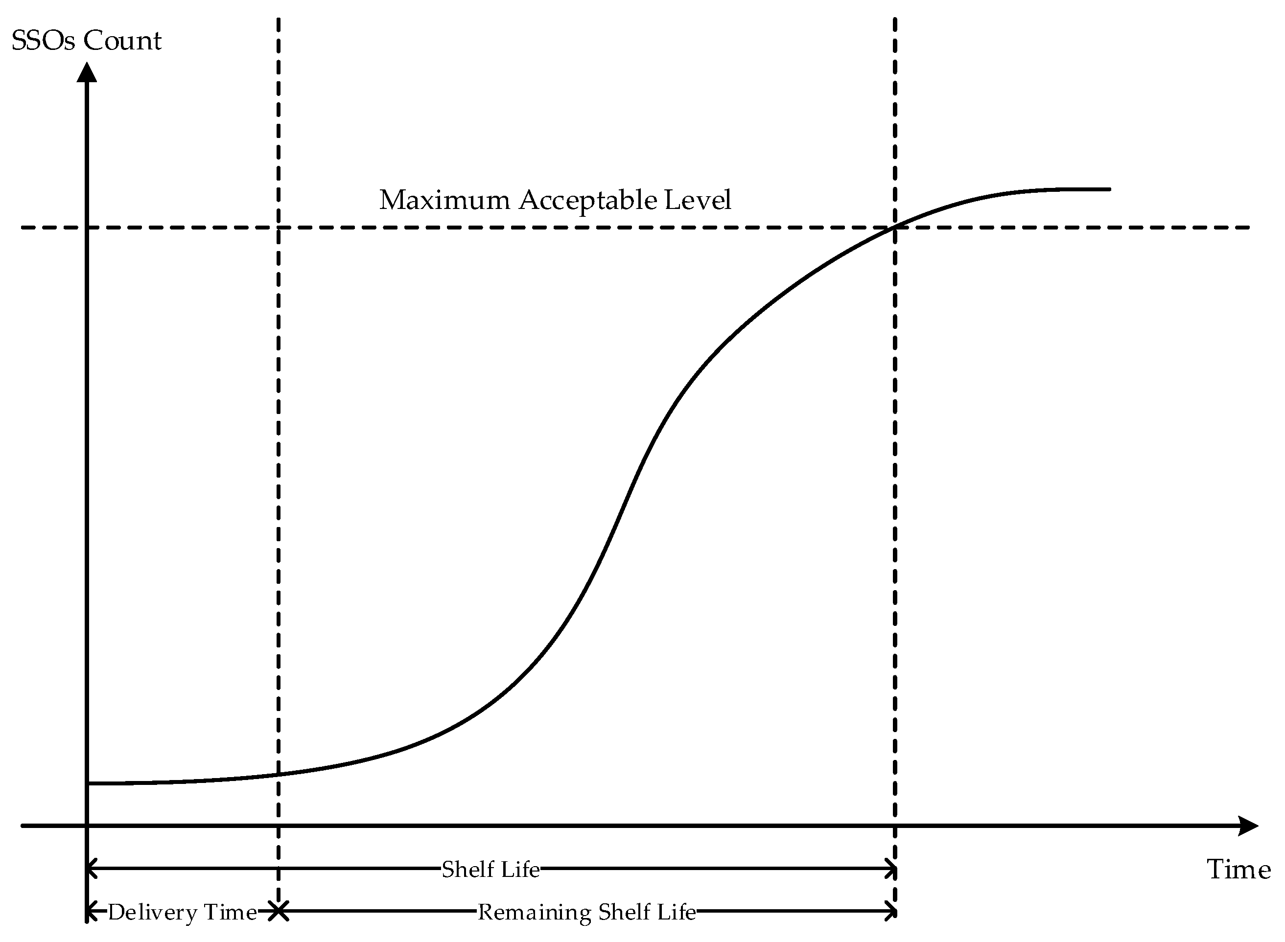
3.3. Food Product Freshness Based on Shelf Life Prediction

Increased temperature can elevate the growth rate of specific spoilage organisms (SSOs) in perishable food products [11]. Therefore, most shelf life prediction models require the temperature of the product over time, as well as product characteristics, to predict the remaining shelf life. Using the temperature prediction method explained in Section 3.1, an accurate estimate of product temperature from the time of vehicle departure from the depot until delivery is possible.

While most studies assume that the remaining shelf life of a product declines at a constant rate over time, the shelf life prediction model provided by Bruckner et al. [5] predicts a nonlinear increase in the number of SSOs in non-isothermal conditions. A product reaches the end of its shelf life when the number of SSOs reaches its maximum acceptable level. The product is not safe for consumption beyond this point and is considered spoiled. The remaining shelf life of food products can be estimated at any point in time, given the initial count of SSOs and characteristics of the food at presumed future storage temperature. Figure 2 shows the number of SSOs over time for a unit of product volume for constant temperature.

The Gompertz model [52] predicts the number of SSOs over time:

$$N\left(t\right)=A+C\ast e^{-e^{-B\left(t-M\right)}}$$

(12)

N (t): SSO count (log₁₀ cfu g⁻¹) at time t,

A: Initial SSO count of the food product at the time it is loaded into a refrigerated vehicle (log₁₀ cfu g⁻¹)

C: The difference between the maximum SSO population level (a constant defined for each type of food product) and the initial SSO count A (log₁₀ cfu g⁻¹)

M: Time at which the maximum growth rate is obtained (h)

B: Relative growth rate at time M (h⁻¹)

The relative growth rate (B) is a function of temperature and is predicted by the Arrhenius equation [53]:

$$ln\left(B\right)=\ln \left(F\right)-\frac{E_a}{R}.\left(\frac{1}{T}\right)$$

(13)

F: Pre-exponential factor describing the number of times two molecules collide

Ea: Activation energy for growth of SSOs (J mol⁻¹)

R: Gas constant (8.314 J mol⁻¹ K⁻¹)

T: Absolute temperature (K)

The freshness of the delivered products at location j (fr_j) can be evaluated using Equation (14) as the percentage of remaining shelf life before distribution to location j, given estimated time and temperature conditions. The remaining shelf life is the amount of time that it will take for the number of SSOs to climb from their current level to the maximum acceptable level.

$$f{r}_j=\frac{Remainingshelflif{e}_j}{shelflif{e}_j}\times 100=\left(1-\frac{deliverytim{e}_j}{shelflif{e}_j}\right)\times 100$$

(14)

3.4. Mathematical Model

The freshness prediction and CO₂ emission modules are integrated with a VRP model to create the MO-SVRP model. The perishable food distribution problem is defined as a directed graph in which a fleet of homogenous vehicles (V), each with a capacity of Q, deliver perishable food from a depot (node 0) to a set of customers (C) using a set of transportation paths (A) which connect the nodes. The order that fulfills the demand of customer i (d_i) must be delivered within the customer’s required time window ([a_i, b_i]). For ease of reference, all notations are given in

Table 2. Notations used in the MO-SVRP model.

Sets:

C = {1, …, n}: set of customers

V = {1, …, v}: set of vehicles

N = {0} ${{\displaystyle \cup }}^{\text{}}$ C: set of depot and customers

A = {(i, j): i, j $\in$ N, and i ≠ j}: set of paths from node i to node j

Parameters:

cij: cost of traveling from node i to node j

tij: travel time from node i to node j

F: fixed dispatching cost

Q: vehicle capacity

di: customer i demand

[ai, bi]: required time window for delivery to customer i

ut: average unloading time for one unit of product

ui: unloading time at customer i, where $u_i$ = $\frac{d_i}{ut}$ and ui ≤ bi − ai

Decision variables:

$y_{ik}$: time that vehicle k arrives at node i

$x_{ijk}$: equals 1 if vehicle k travels from node i to node j, 0 otherwise

$l_{ijk}$: units of product carried by vehicle k between nodes i and j

.

The MO-SVRP model is formulated as a multi-objective mixed-integer program, and the mathematical formulation is as follows:

$$Minimize{Z}_1={\sum }_{kϵV}{\sum }_{iϵN}{\sum }_{jϵN}{c}_{ij}{x}_{ijk}+{\sum }_{j\in C}{\sum }_{k\in V}F{x}_{0jk}$$

(15)

$$Maximize{Z}_2={\sum }_{iϵC}f{r}_i\frac{d_i}{{\sum }_{j\in C}{d}_j}$$

(16)

$$Minimize{Z}_3={\sum }_{kϵV}{E}_k$$

(17)

Subject to

$$\begin{array}{lll}{\sum }_{kϵV}{\sum }_{jϵN}{x}_{ijk}=1& & \forall i\in C,i\ne j\end{array}$$

(18)

$$\begin{array}{lll}{\sum }_{iϵC}{d}_i{\sum }_{jϵN}{x}_{ijk}\le Q& & \forall k\in V,i\ne j\end{array}$$

(19)

$$\begin{array}{lll}{\sum }_{j\in C}{x}_{0jk}\le 1& & \forall k\in V\end{array}$$

(20)

$$\begin{array}{lll}{\sum }_{iϵN}{x}_{ihk}-{\sum }_{jϵN}{x}_{hjk}=0& & \forall h\in N,k\in V\end{array}$$

(21)

$$\begin{array}{lll}{\sum }_{j\in N}{\sum }_{k\in V}{l}_{jik}-{\sum }_{j\in N}{\sum }_{k\in V}{l}_{ijk}=d_i& & \forall i\in C\end{array}$$

(22)

$$\begin{array}{lll}{y}_{ik}+u_i+t_{ij}-M\left(1-x_{ijk}\right)\le y_{jk}& & \forall i\in C,j\in N,k\in V\end{array}$$

(23)

$$\begin{array}{lll}{t}_{0j}\le y_{jk}+M\left(1-x_{0jk}\right)& & \forall j\in C,k\in V\end{array}$$

(24)

$$\begin{array}{lll}{a}_i\le y_{ik}\le b_i& & \forall i\in C\end{array}$$

(25)

$$\begin{array}{lll}{l}_{ijk}\le \left(Q-d_i\right)x_{ijk}& & \forall i\in N,j\in N,k\in V\end{array}$$

(26)

$$\begin{array}{lll}{d}_j{x}_{ijk}\le l_{ijk}& & \forall i\in N,j\in C,k\in V\end{array}$$

(27)

$$\begin{array}{lll}{y}_{ik}\ge 0& & \forall i\in C,k\in V\end{array}$$

(28)

$$\begin{array}{lll}{l}_{ijk}\ge 0& & \forall i\in N,j\in C,k\in V\end{array}$$

(29)

$$\begin{array}{lll}{x}_{ijk}ϵ\left\{0,1\right\}& & \forall i\in C,k\in V\end{array}$$

(30)

The first objective (Equation (15)) minimizes transportation costs, including the cost of traveling between customer locations as the first term and dispatching costs associated with the fixed costs of using a vehicle in the distribution plan as the second term. The second objective (Equation (16)) maximizes the total freshness of the delivered products at each customer location. The third objective (Equation (17)) minimizes total CO₂ emissions generated by refrigerated vehicles during transit and unloading. Equation (18) ensures that each customer location can be visited by only one vehicle. Equation (19) prevents the load carried between two locations from being greater than the capacity of the vehicle. A vehicle can only leave the depot once (Equation (20)), and if a vehicle arrives at a location, it must also leave that location (Equation (21)). The amount of cargo unloaded at a customer location must equal that customer’s demand (Equation (22)). Equation (23) ensures that a customer cannot be visited prior to the time that the previous customer is visited plus the unloading and travel times between these two customers. Similarly, Equation (24) prevents the first customer from being visited earlier than the time required to travel from the depot to that customer’s location. Deliveries must occur within customers’ required time windows (Equation (25)). A vehicle’s load after leaving a customer location must be less than or equal to the capacity of the vehicle minus the demand of the visited customer (Equation (26)), and Equation (27) ensures that the load carried between two customer locations is at least equal to the demand of the next customer. Equations (28) and (29) prevent the arrival time and the load carried by a vehicle from taking negative values, and Equation (30) defines a vehicle’s path as a binary variable.

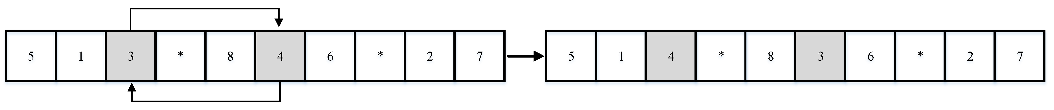
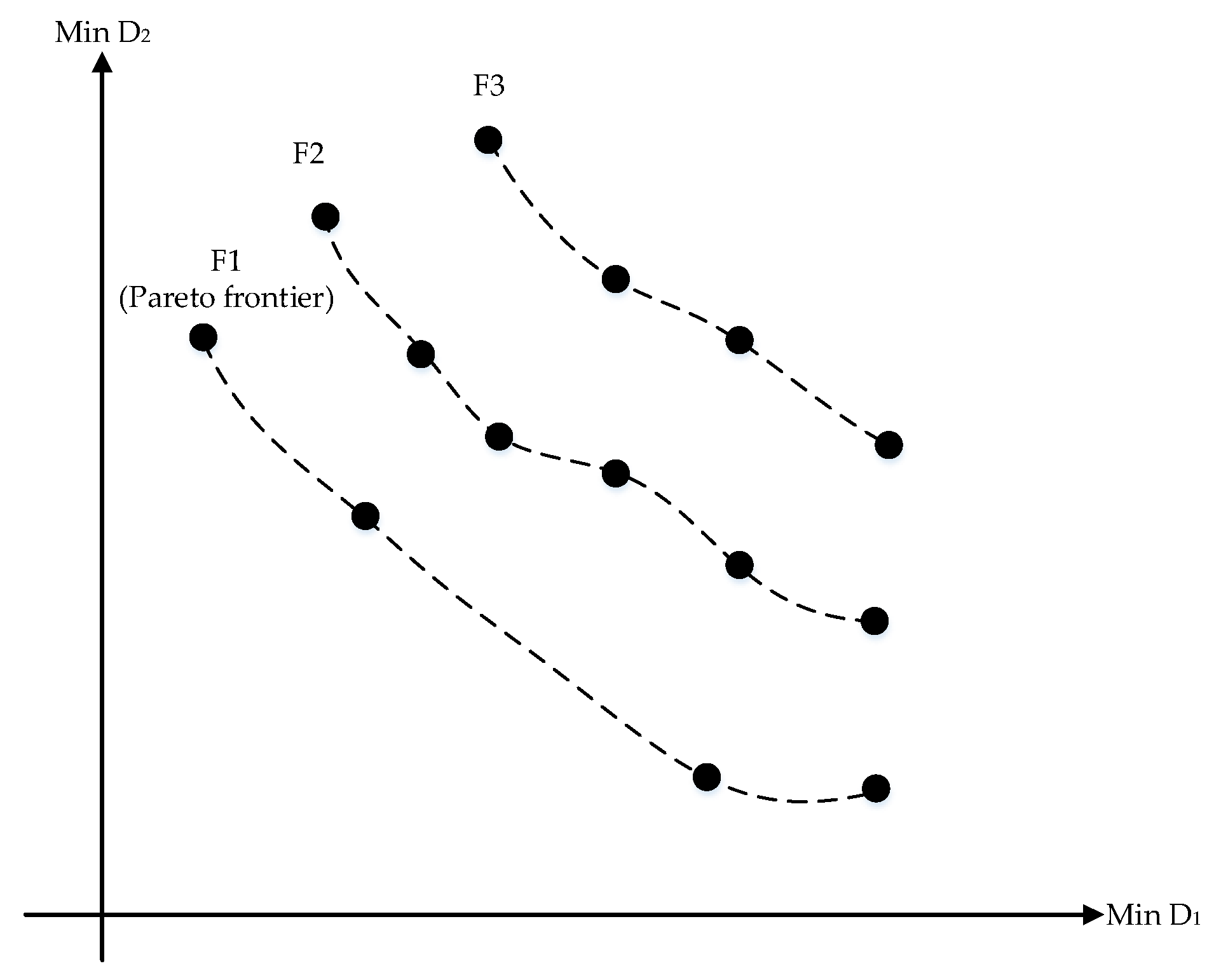
4. Solution Procedure

The MO-SVRP model presented in the previous section is difficult to solve. Even a VRP problem with a single objective and fewer parameters and variables is categorized as an NP-hard problem [24,54]. Consequently, a meta-heuristic approach was applied to solve the problem in a reasonable time. NSGA-II is an efficient and widely applied meta-heuristic approach introduced by Deb et al. [55] as a search technique for finding optimal solutions to multi-objective problems. This algorithm works based on iterative improvements in the pool of solutions’ quality. In each iteration, genetic algorithm operators create offspring from the existing pool of solutions, and the solutions in this new pool are sorted based on the non-dominated sorting algorithm and crowding distance index. The top solutions are then selected for the next iteration. This section describes how this approach has been applied to solve the MO-SVRP.

In the NSGA-II algorithm, a “chromosome” represents a solution that assigns a list of customers to each vehicle in a particular delivery sequence. Each chromosome is an array consisting of n + v − 1 elements, in which n represents the number of customers and v represents the number of vehicles. An example is given in Figure 3. There are v − 1 special characters in the array (“*” in Figure 3), which divide the array into v sections (i.e., one section for each vehicle). The n remaining elements of the array are integer values from 1 to n, each of which is assigned to a customer. Thus, the sections between two special characters are lists of customers assigned to each vehicle, and the order of these numbers represents the delivery sequence.

Initially, n customers and v − 1 special characters are randomly assigned to p chromosomes, where p is the size of the pool of solutions. Then, crossover and mutation operators are used to generate new solutions as the algorithm iterates.

The single point crossover operator is used to generate P_c chromosomes from the previous pool of solutions. Figure 4 provides an example, in which the first three elements the parent chromosomes are swapped to create two new offspring.

The crossover procedure is followed by a repair procedure [25], which is applied to fix chromosomes that have duplicated or missing customers or special characters. An example is shown in Figure 5.

P_m solutions are then randomly selected from the previous pool of solutions. The locations of two randomly selected elements from each chromosome are swapped, as shown in the example in Figure 6.

The solutions are then categorized based on the number of solutions that dominate them. The front i (F_i, i ϵ K, where K is the number of categories) includes the solutions with rank i dominated by i-1 other solutions. Solutions that cannot be dominated by any other solutions from their pool comprise the Pareto frontier. Figure 7 shows how the pool of solutions in domains D1 and D2 is categorized in three fronts.

Crowding distance is an estimate of the density of solutions around a particular solution in a front. The value of crowding distance for a particular solution is the summation of distances of the solutions with the neighboring solutions of the same front. Equations (31) and (32) show the mathematical equations by which crowding distance is calculated.

$$d_i^j=\left|f_j^{i+1}-f_j^{i-1}\right|$$

(31)

$d_i^j$: Distance of solution i from its neighbors in domain j

$f_j^i$: Value of function f for solution i in domain j

$$d_i={\sum }_{j\in D}{d}_i^j$$

(32)

$d_i$: Crowding distance of solution i

D: Set of the problem domains

In each iteration, binary tournament selection is applied to sort the solutions, first based on their ranks, and then based on their crowding distance.

The NSGA-II main loop consists of offspring generation and ranking and sorting modules. Algorithm 1 presents a pseudocode that illustrates an iteration of the NSGA-II algorithm. At the end of each iteration, solutions with rank 1 are stored as Pareto-frontier.

Algorithm 1 NSGA-II main loop pseudocode

p = population of randomly generated chromosomes with size pops for i = 1 to Max number of iterations do   for j =1 to (pc ÷ 2) do     c1 = 1st randomly chosen parent chromosome     c2 = 2nd randomly selected parent chromosome     popc = append crossover (c1, c2)   for k = 1 to pm do     m = a randomly chosen parent chromosome     popm = append mutate (m)   pop = merge (p, popc, popm)   function (non-dominated sorting (input: pop))     return: Rank of chromosomes   function (crowding distance (input: pop, rank))     return: crowding distance value for each chromosome   function (sort population (input: pop, rank, crowding distance))     return: sorted pop based on 1) rank, 2) crowding distance   pop = store only the top pop and truncate the others   function (non-dominated sorting (input: pop))     return: Rank of chromosomes   function (crowding distance (input: pop, rank))     return: crowding distance value for each chromosome   function (sort population (input: pop, rank, crowding distance))     return: sorted pop based on 1) rank, 2) crowding distance   Pareto_frontier = chromosomes with rank 1   Go to the next iteration if the stopping criteria are not met

5. Computational Results and Discussion

5.1. Performance of the Solution Method

First, the performance of the NGSA-II solution algorithm in solving the MO-SVRP was tested on Solomon’s datasets [56], which are widely applied to measure the quality of solutions for a VRP. The geographical distribution of the visiting location has a substantial impact on the performance of the VRP solution algorithm. So, these instances were provided in three categories: R, C, and RC, representing randomly generated, clustered, and mixed generated geographical data, respectively. Within these three categories, the MO-SVRP was solved for small instances (25 customers) and large instances (100 customers). However, the solutions should be compared with a competing algorithm to verify the efficiency and accuracy of the NGSA-II. Thus, weighted simulated annealing (w-SA) was used to solve the single objective weighted problem. According to the L1 metric method, the inverse of the optimum solution for each objective was used as the weight of the objectives in a single weighted objective function [23].

The NSGA-II and w-SA algorithms were coded in Python and run on a computer with 3.10 GHz Intel Core i9 CPU, 64 GB of RAM, and Windows 10 operating system. The parameter values that were used are given in

Table 3. Test problem and solution algorithm parameters.

w-SA Parameters	Value	NSGA-II Parameters	Value	Test Problem Parameters	Value
Initial temperature	20	Population size	30	Vehicle speed (km h−1)	15
Damping rate	0.99	Crossover rate	0.7	Product shelf life (h)	2880
		Mutation rate	0.4	Fixed cost per vehicle ($)	1000
				Transportation cost ($ km−1)	1.5
				Service time (minute)	10 * 90 **
				Vehicle capacity (kg)	200

* for R and RC test problems, ** for C test problems.

. The algorithms terminate when the solutions in the Pareto front (for NSGA-II) or the optimum solution (for w-SA) do not improve after a certain number of iterations, which depends on the size of the problem.

In

Table 4. Comparison of the performance of weighted simulated annealing (w-SA) and NSGA-II.

Test Problem	w-SA			NSGA-II			Gap
	Costs ($)	Freshness (%)	CO2 (lbs × 103)	Costs ($)	Freshness (%)	CO2 (lbs × 103)	Costs ($)	Freshness (%)	CO2 (lbs × 103)
R101 (25)	5233	89%	4164	4,886	95%	3848	6.6%	4.8%	17.5%
R101 (100)	13,450	90%	48,042	12,356	94%	45,026	8.1%	2.3%	6.3%
C101 (25)	3065	90%	2452	2761	96%	2305	9.9%	6.7%	6.0%
C101 (100)	10,655	92%	39,787	9452	94%	38,564	11.3%	2.2%	3.1%
RC101 (25)	3318	90%	3,075	3027	92%	2684	8.8%	4.6%	12.7%
RC101 (100)	11,569	91%	47,666	10,335	93%	42,597	10.7%	4.5%	2.4%

, the column “w-SA” provides the values of each of the three objective functions for the best solution to each test problem instance. The values of the objective functions in the “NSGA-II” column correspond to the best solution that was found among the Pareto front solutions for each objective. The gap shows the difference between the objective values divided by the best value generated by these algorithms.

The results in Table 4 show that, on average, NSGA-II provides solutions that are 9.2%, 4.2%, and 8.0% better than w-SA in terms of cost, freshness, and emission objectives, respectively. The advantage of NSGA-II over w-SA is more pronounced for the cost objective when the size of the problem increases, or when the customers are more geographically clustered (i.e., the gap is largest for the C instances).

5.2. Optimality Analysis

Balancing cost, freshness, and emission objectives is necessary to improve the sustainability of perishable food distribution networks. The results in

Table 5. Impact of choosing a non-dominated solution on the optimality of the transportation costs, freshness, and emissions for R101(25) instance.

Optimality	No. of Vehicles	Costs ($)	Freshness (%)	CO2 (lbs × 103)
Cost	7	4886 (*)	55% (42% gap)	3997 (4% gap)
Freshness	8	112,123 (95% gap)	95% (*)	66,413 (94% gap)
Emission	7	5723 (14% gap)	56% (41% gap)	3848 (*)
Final solution	7	10,213 (52% gap)	75% (21% gap)	8892 (57% gap)

* optimum.

demonstrate the conflicting nature of the three objectives: if the MO-SVRP problem is solved for a single objective, the values of the other two objective functions deviate significantly from optimality. Because the traveled distance is the primary driver of transportation cost and emissions, it is unsurprising that the emissions objective in the cost-optimal solution has only a 4% gap with the emission-optimal solution, and cost objective in the emission-optimal solution is only 14% higher than in the cost-optimal solution. However, keeping perishable products fresh requires faster delivery and fewer stops, which means that the vehicles may not be full. This increases the total traveled distance, which increases transportation cost and energy consumption, such that a solution that preserves 95% of the product’s freshness results in 95% and 94% optimality gaps for cost and emissions objectives, respectively. In contrast, when a solution is cost- or emissions-optimal, freshness is 42% and 41% less than optimal, respectively.

Most likely, there is more than one non-dominated solution in the Pareto frontier. So, a final solution that properly reflects the impact of all the objectives is chosen from the non-dominated set of solutions in the Pareto frontier. To choose a final solution, the approach developed by Bortolini et al. [32] was adapted. The presented method only ranks the solutions based on their distance to the optimum objective values, and other factors such as decision-maker priorities are not reflected in this method.

$$Min{\theta }_l$$

(33)

$${\theta }_l=\frac{{\alpha }_l}{{\alpha }_l^{\ast }}.\frac{{\beta }_1^{\ast }}{{\beta }_1}.\frac{{\gamma }_l}{{\gamma }_l^{\ast }}$$

(34)

${\theta }_l$: Represents a single calculated value for a solution l in Pareto frontier

${\alpha }_l$: Value of the first objective function for solution l

${\alpha }_l^{\ast }$: Optimum value of the first objective function for solution l

${\beta }_l$: Value of the second objective function for solution l

${\beta }_l^{\ast }$: Optimum value of the second objective function for solution l

${\gamma }_l$: Value of the third objective function for solution l

${\gamma }_l^{\ast }$: Optimum value of the third objective function for solution l

As shown in Table 5, the optimality gaps for each objective in the final solution are 52%, 57%, and 21% for cost, emissions, and freshness, respectively. When the only objective is to maximize freshness, the refrigerated vehicles are likely carrying loads that are far smaller than their capacity, rather than consolidating customer orders to ensure fast delivery and few delivery stops. In this scenario, the vehicles’ traveled distances are very high, and consequently, distribution costs and CO₂ emission are at their highest level. Consolidating orders and increasing vehicle capacity utilization provides a substantial improvement in the cost and emission objectives, and the gaps of these objectives associated with the final solution reflect this.

5.3. Sensitivity to Shelf Life

To generate the results presented in the previous sections, it was assumed that the products have similar characteristics and the same shelf life (i.e., 2880 h). In reality, perishable products’ shelf life can range from 168 h for highly perishable products, such as tomatoes, to 1440 h for moderately perishable products, such as oranges, and 2880 h for products with low perishability, such as apples. Therefore, the sensitivity of the MO-SVRP model to long, medium and short shelf life scenarios was analyzed. The final values of the three objectives for these shelf life scenarios are shown in

Table 6. Final solutions for transportation costs, freshness, and CO₂ emissions for products with different shelf life values (for R101(25) instance).

Shelf Life (h)	Costs ($)	Freshness (%)	CO2 (lbs × 103)
168	13,522	62%	12,916
1440	11,390	71%	10,662
2880	10,213	75%	8892

. The results emphasize the increase in cost and energy that is required to distribute more perishable items, as well as the loss of freshness for shorter shelf-life products. These results suggest that distributors should consider investing more money and time on improving container isolation and the efficiency of the diesel engine to reduce energy consumption and preserve quality when distributing products with a shorter shelf life. These results are compatible with the findings of Bortolini et al. [32] in which it was illustrated that products with lower shelf life have higher operating costs and produce a higher carbon footprint.

5.4. Sensitivity to Temperature Setting

Although there are recommended temperature ranges for perishable product storage, determining the specific temperature setting for a refrigerated shipping container can be challenging. Lower temperature settings preserve product quality, but this requires more energy. Therefore, the sensitivity of the MO-SVRP model to various temperature settings was assessed by solving the R101(25) instance at temperature settings between 263–269 degrees Kelvin (14–25 °F) in two-degree increments.

Table 7. Final solutions for transportation costs, freshness, and CO₂ emissions for different container temperature settings (for R101(25) instance).

Temperature (°K)	Costs ($)	Freshness (%)	CO2 (lbs × 103)
263	10,213	75%	8892
265	10,526	72%	8556
267	11,013	68%	8436
269	11,596	60%	8301

shows that the final solutions for the three sustainability objectives for different temperature settings inside the container. Increasing the temperature setting from 263 °K to 269 °K causes a 15% reduction in product freshness (from 75% to 60%). Because the MO-SVRP recommends faster delivery to compensate for the loss in quality that results from an increase in temperature, the transportation distance and cost tend to increase at higher temperature settings. However, the effect of an increased temperature setting on emissions is more complex. On one hand, transportation consumes more energy due to the increase in traveled distance. On the other hand, energy consumption for refrigeration decreases. This leads to a decrease in overall energy consumption throughout distribution.

6. Conclusions and Future Research

In this paper, the VRP is extended to consider the perishability of the food products and refrigerated vehicles’ CO₂ emissions in a multi-objective framework. The model addresses sustainability concerns associated with the perishable food distribution problem in a mathematical model by minimizing transportation costs and CO₂ emissions and maximizing product freshness. Integrating a temperature estimation model provides accurate predictions of refrigeration-related emissions and product quality loss during distribution. The presented MO-SVRP model was solved using an adapted NSGA-II algorithm, and the performance of the solution algorithm was tested and verified against the w-SA algorithm over the Solomon [56] data sets.

The results of the analysis revealed that the sustainability objectives are conflicting, such that optimizing one objective can degrade the other two objectives. In particular, optimizing the freshness objective leads to a solution in which deploying all the available vehicles to minimize delivery time and the quality-deteriorating effect of temperature abuses at the delivery locations. Therefore, the optimality gaps in distribution costs and CO₂ emission objectives are high when only the freshness objective is optimized. Furthermore, when vehicles are carrying highly perishable products, the MO-SVRP model recommends faster delivery and fewer stops, which increases energy consumption and distribution costs. Sensitivity analysis over different temperature settings inside the shipping container indicates that even small increments in the temperature settings can have a huge impact on CO₂ emissions and freshness objectives. This sensitivity analysis can be a helpful tool to determine the best temperature setting to achieve sustainability goals.

This paper is mainly focused on presenting a methodology to accurately measure and optimize sustainability goals in the distribution of perishable food products. It is highly recommended to apply the methodology in practice to evaluate the sustainability goals with respect to the real-world parameters and constraints. The methodology of this research is limited to the single product distribution system with single compartment refrigerated vehicles. Considering the growth in the application of multi-compartment refrigerated vehicles to distribute multiple types of products with one vehicle, it would an interesting expansion for this study to measure and optimize sustainability objectives for perishable food distribution with multi-compartment refrigerated vehicles in which each food product has different perishability parameters and the compartments of the refrigerated vehicles can be set to different temperatures.

The outcomes of this research highlight the necessity of integrating and accurately estimating multiple influential factors that impact sustainability in a perishable food distribution network to find solutions that are cost-effective, reduce food waste, and decrease emissions generated by refrigerated vehicles.

References

1. Todorovic, V.; Maslaric, M.; Bojic, S.; Jokic, M.; Mircetic, D.; Nikolicic, S. Solutions for more sustainable distribution in the short food supply chains. Sustainability 2018, 10, 3481. [Google Scholar] [CrossRef]
2. James, S.J.; James, C.; Evans, J.A. Modelling of food transportation systems—A review. Int. J. Refrig. 2006, 29, 947–957. [Google Scholar] [CrossRef]
3. Tarantilis, C.D.; Kiranoudis, C.T. Distribution of fresh meat. J. Food Eng. 2002, 51, 85–91. [Google Scholar] [CrossRef]
4. Yang, S.; Xiao, Y.; Zheng, Y.; Liu, Y. The Green Supply Chain Design and Marketing Strategy for Perishable Food Based on Temperature Control. Sustainability 2017, 9, 1511. [Google Scholar] [CrossRef] [Green Version]
5. Bruckner, S.; Albrecht, A.; Petersen, B.; Kreyenschmidt, J. A predictive shelf life model as a tool for the improvement of quality management in pork and poultry chains. Food Control. 2013, 29, 451–460. [Google Scholar] [CrossRef]
6. Gharehyakheh, A.; Krejci, C.; Cantu, J.; Rogers, J. Dynamic Shelf-Life Prediction System to Improve Sustainability in Food Banks. In Proceedings of the 2019 IISE Annual Conference, Orlando, FL, USA, 18–21 May 2019. [Google Scholar]
7. Göransson, M.; Jevinger, A.; Nilsson, J. Shelf-life variations in pallet unit loads during perishable food supply chain distribution. Food Control. 2018, 84, 552–560. [Google Scholar] [CrossRef]
8. Kreyenschmidt, J.; Hübner, A.; Beierle, E.; Chonsch, L.; Scherer, A.; Petersen, B. Determination of the shelf life of sliced cooked ham based on the growth of lactic acid bacteria in different steps of the chain. J. Appl. Microbiol. 2010, 108, 510–520. [Google Scholar] [CrossRef]
9. Novaes, A.G.N.; Lima, O.F., Jr.; de Carvalho, C.C.; Bez, E.T. Thermal performance of refrigerated vehicles in the distribution of perishable food. Pesqui. Oper. 2015, 35, 251–284. [Google Scholar] [CrossRef] [Green Version]
10. Osvald, A.; Stirn, L.Z. A vehicle routing algorithm for the distribution of fresh vegetables and similar perishable food. J. Food Eng. 2008, 85, 285–295. [Google Scholar] [CrossRef]
11. Mercier, S.; Villeneuve, S.; Mondor, M.; Uysal, I. Time–Temperature Management Along the Food Cold Chain: A Review of Recent Developments. Compr. Rev. Food Sci. Food Saf. 2017, 16, 647–667. [Google Scholar] [CrossRef]
12. Food Waste and Loss. United States Department of Agriculture. 2015. Available online: https://www.fda.gov/food/consumers/food-waste-and-loss (accessed on 9 February 2020).
13. Gustavsson, J.; Cederberg, C.; Sonesson, U.; van Otterdijk, R.; Meybeck, A. Global Food Losses and Food Waste: Extent, Causes and Prevention; Swedish Institute for Food and Biotechnology (SIK): Gothenburg, Sweden, 2011. [Google Scholar]
14. Young, L. Our Biggest Problem? We’re Wasting Food. Can. Grocer 2012. Available online: http://www.canadiangrocer.com/top-stories/what-a-waste-19736 (accessed on 6 April 2020).
15. Scharff, R.L. Economic burden from health losses due to foodborne illness in the united states. J. Food Prot. 2012, 75, 123–131. [Google Scholar] [CrossRef] [PubMed]
16. CDC. Burden of Foodborne Illness: Findings. In Centers for Disease Control and Prevention; 2011. Available online: https://www.cdc.gov/foodborneburden/2011-foodborne-estimates.html (accessed on 10 April 2020).
17. Stellingwerf, H.M.; Kanellopoulos, A.; van der Vorst, J.G.A.J.; Bloemhof, J.M. Reducing CO2 emissions in temperature-controlled road transportation using the LDVRP model. Transp. Res. Part D Transp. Environ. 2018, 58, 80–93. [Google Scholar] [CrossRef]
18. Adekomaya, O.; Jamiru, T.; Sadiku, R.; Huan, Z. Sustaining the shelf life of fresh food in cold chain–A burden on the environment. Alex. Eng. J. 2016, 55, 1359–1365. [Google Scholar] [CrossRef] [Green Version]
19. Ketzenberg, M.; Bloemhof, J.; Gaukler, G. Managing Perishables with Time and Temperature History. Prod. Oper. Manag. 2015, 24, 54–70. [Google Scholar] [CrossRef]
20. Gharehyakheh, A.; Cantu, J.; Krejci, C.; Rogers, J. Sustainable delivery system in a temperature controlled supply chain. In Proceedings of the IISE Annual Conference and Expo 2018, Orlando, FL, USA, 19–22 May 2018; pp. 1534–1539. [Google Scholar]
21. Tassou, S.A.; De-Lille, G.; Ge, Y.T. Food transport refrigeration–Approaches to reduce energy consumption and environmental impacts of road transport. Appl. Therm. Eng. 2009, 29, 1467–1477. [Google Scholar] [CrossRef] [Green Version]
22. Wang, X.; Wang, M.; Ruan, J.; Zhan, H. The Multi-objective Optimization for Perishable Food Distribution Route Considering Temporal-spatial Distance. Procedia Comput. Sci. 2016, 96, 1211–1220. [Google Scholar] [CrossRef] [Green Version]
23. Rahbari, A.; Nasiri, M.M.; Werner, F.; Musavi, M.; Jolai, F. The vehicle routing and scheduling problem with cross-docking for perishable products under uncertainty: Two robust bi-objective models. Appl. Math. Model. 2019, 70, 605–625. [Google Scholar] [CrossRef]
24. Xiao, Y.; Zhao, Q.; Kaku, I.; Xu, Y. Development of a fuel consumption optimization model for the capacitated vehicle routing problem. Comput. Oper. Res. 2012, 39, 1419–1431. [Google Scholar] [CrossRef]
25. Musavi, M.M.; Bozorgi-Amiri, A. A multi-objective sustainable hub location-scheduling problem for perishable food supply chain. Comput. Ind. Eng. 2017, 113, 766–778. [Google Scholar] [CrossRef]
26. Chen, H.K.; Hsueh, C.F.; Chang, M.S. Production scheduling and vehicle routing with time windows for perishable food products. Comput. Oper. Res. 2009, 36, 2311–2319. [Google Scholar] [CrossRef]
27. Ghezavati, V.R.; Hooshyar, S.; Tavakkoli-Moghaddam, R. A Benders’ decomposition algorithm for optimizing distribution of perishable products considering postharvest biological behavior in agri-food supply chain: A case study of tomato. Cent. Eur. J. Oper. Res. 2017, 25, 29–54. [Google Scholar] [CrossRef]
28. Albrecht, W.; Steinrücke, M. Coordinating continuous-time distribution and sales planning of perishable goods with quality grades. Int. J. Prod. Res. 2018, 56, 2646–2665. [Google Scholar] [CrossRef]
29. Ahumada, O.; Villalobos, J. A tactical model for planning the production and distribution of fresh produce. Ann. Oper. Res. 2011, 190, 339–358. [Google Scholar] [CrossRef]
30. Farahani, P.; Grunow, M.; Günther, H.O. Integrated production and distribution planning for perishable food products. Flex. Serv. Manuf. J. 2012, 24, 28–51. [Google Scholar] [CrossRef]
31. Hsu, C.I.; Hung, S.F.; Li, H.C. Vehicle routing problem with time-windows for perishable food delivery. J. Food Eng. 2007, 80, 465–475. [Google Scholar] [CrossRef]
32. Bortolini, M.; Faccio, M.; Ferrari, E.; Gamberi, M.; Pilati, F. Fresh food sustainable distribution: Cost, delivery time and carbon footprint three-objective optimization. J. Food Eng. 2016, 174, 56–67. [Google Scholar] [CrossRef]
33. Amorim, P.; Almada-Lobo, B. The impact of food perishability issues in the vehicle routing problem. Comput. Ind. Eng. 2014, 67, 223–233. [Google Scholar] [CrossRef]
34. Amorim, P.; Günther, H.O.; Almada-Lobo, B. Multi-objective integrated production and distribution planning of perishable products. Int. J. Prod. Econ. 2012, 138, 89–101. [Google Scholar] [CrossRef]
35. Hsu, C.I.; Chen, W.T.; Wu, W.J. Optimal delivery cycles for joint distribution of multi-temperature food. Food Control. 2013, 34, 106–114. [Google Scholar] [CrossRef]
36. Hsiao, Y.-H.; Chen, M.-C.; Chin, C.-L. Distribution planning for perishable foods in cold chains with quality concerns: Formulation and solution procedure. Trends Food Sci. Technol. 2017, 61, 80–93. [Google Scholar] [CrossRef]
37. Gallo, A.; Accorsi, R.; Baruffaldi, G.; Manzini, R. Designing sustainable cold chains for long-range food distribution: Energy-effective corridors on the Silk Road Belt. Sustainability 2017, 9, 2044. [Google Scholar] [CrossRef] [Green Version]
38. Wang, S.; Tao, F.; Shi, Y. Optimization of Location-Routing Problem for Cold Chain Logistics Considering Carbon Footprint. Int. J. Environ. Res. Public Health 2018, 15, 86. [Google Scholar] [CrossRef] [Green Version]
39. Bektaş, T.; Laporte, G. The pollution-routing problem. Transp. Res. Part B Methodol. 2011, 45, 1232–1250. [Google Scholar] [CrossRef]
40. Accorsi, R.; Gallo, A.; Manzini, R. A climate driven decision-support model for the distribution of perishable products. J. Clean. Prod. 2017, 165, 917–929. [Google Scholar] [CrossRef]
41. Govindan, K.; Jafarian, A.; Khodaverdi, R.; Devika, K. Two-echelon multiple-vehicle location-routing problem with time windows for optimization of sustainable supply chain network of perishable food. Int. J. Prod. Econ. 2014, 152, 9–28. [Google Scholar] [CrossRef]
42. Molina, J.C.; Eguia, I.; Racero, J.; Guerrero, F. Multi-objective Vehicle Routing Problem with Cost and Emission Functions. Procedia Soc. Behav. Sci. 2014, 160, 254–263. [Google Scholar] [CrossRef] [Green Version]
43. Wang, F.; Lai, X.; Shi, N. A multi-objective optimization for green supply chain network design. Decis. Support Syst. 2011, 51, 262–269. [Google Scholar] [CrossRef]
44. Devapriya, P.; Ferrell, W.; Geismar, N. Integrated production and distribution scheduling with a perishable product. Eur. J. Oper. Res. 2017, 259, 906–916. [Google Scholar] [CrossRef]
45. Khalili-Damghani, K.; Abtahi, A.R.; Ghasemi, A. A New Bi-objective Location-routing Problem for Distribution of Perishable Products: Evolutionary Computation Approach. J. Math. Model. Algorithms Oper. Res. 2015, 14, 287–312. [Google Scholar] [CrossRef]
46. Nakandala, D.; Lau, H.; Zhang, J. Cost-optimization modelling for fresh food quality and transportation. Ind. Manag. Data Syst. 2016, 116, 564–583. [Google Scholar] [CrossRef]
47. Soysal, M.; Bloemhof-Ruwaard, J.M.; van der Vorst, J.G.A.J. Modelling food logistics networks with emission considerations: The case of an international beef supply chain. Int. J. Prod. Econ. 2014, 152, 57–70. [Google Scholar] [CrossRef]
48. Validi, S.; Bhattacharya, A.; Byrne, P.J. A case analysis of a sustainable food supply chain distribution system—A multi-objective approach. Int. J. Prod. Econ. 2014, 152, 71–87. [Google Scholar] [CrossRef] [Green Version]
49. Accorsi, R.; Baruffaldi, G.; Manzini, R. Picking efficiency and stock safety: A bi-objective storage assignment policy for temperature-sensitive products. Comput. Ind. Eng. 2018, 115, 240–252. [Google Scholar] [CrossRef]
50. Gharehyakheh, A.; Tavakkoli-Moghaddam, R. A fuzzy solution approach for a multi-objective integrated production-distribution model with multi products and multi periods under uncertainty. Manag. Sci. Lett. 2012, 2, 2425–2434. [Google Scholar] [CrossRef]
51. Holdsworth, S.D.; Simpson, R. Thermal Processing of Packaged Foods; Springer: Cham, Germany, 2016; Volume 284. [Google Scholar]
52. Gibson, A.M.; Bratchell, N.; Roberts, T.A. The effect of sodium chloride and temperature on the rate and extent of growth of Clostridium botulinum type A in pasteurized pork slurry. J. Appl. Bacteriol. 1987, 62, 479–490. [Google Scholar] [CrossRef]
53. Arrhenius, S. Über die Reaktionsgeschwindigkeit bei der Inversion von Rohrzucker durch Säuren. Z. Phys. Chem. 1889, 4, 226–248. [Google Scholar]
54. Savelsbergh, M.W.P. Local search in routing problems with time windows. Ann. Oper. Res. 1985, 4, 285–305. [Google Scholar] [CrossRef] [Green Version]
55. Deb, K.; Pratap, A.; Agarwal, S.; Meyarivan, T. A fast and elitist multiobjective genetic algorithm: NSGA-II. IEEE Trans. Evol. Comput. 2002, 6, 182–197. [Google Scholar] [CrossRef] [Green Version]
56. Solomon, M.M. Vehicle Routing and Scheduling with Time Windows Constraints: Models and Algorithms. Ph.D. Thesis, University of Pennsylvania, Philadelphia, PA, USA, 1984. [Google Scholar]
Figure 1. Integrated structure of multi-objective sustainable vehicle routing problem (MO-SVRP) model.
Sustainability 12 06668 g001
Figure 2. The growth rate of specific spoilage organisms (SSOs) over time at a constant temperature.
Sustainability 12 06668 g002
Figure 3. Non-dominated sorting genetic algorithm (NSGA-II) chromosome encoded as a MO-SVRP solution.
Sustainability 12 06668 g003
Figure 4. Crossover operation.
Sustainability 12 06668 g004
Figure 5. Repair procedure for crossover operation.
Sustainability 12 06668 g005
Figure 6. Mutation operator.
Sustainability 12 06668 g006
Figure 7. Rank of chromosomes in one iteration (F1 is Pareto frontier).
Sustainability 12 06668 g007