Identification of Roof Surfaces from LiDAR Cloud Points by GIS Tools: A Case Study of Lučenec, Slovakia

 , , , and
Abstract
:1. Introduction
2. Materials and Methods
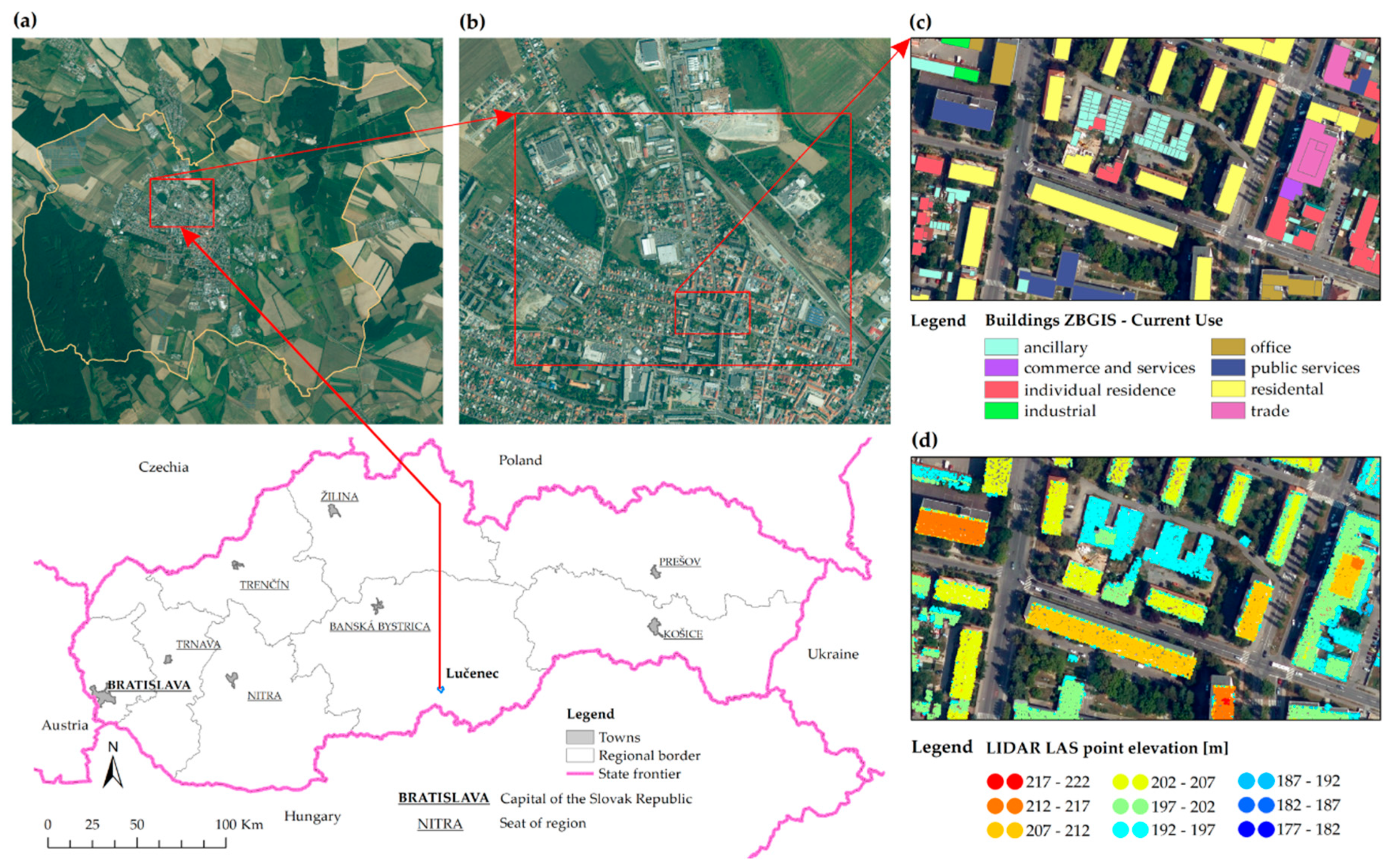
2.1. Study Area
2.2. Data Sources
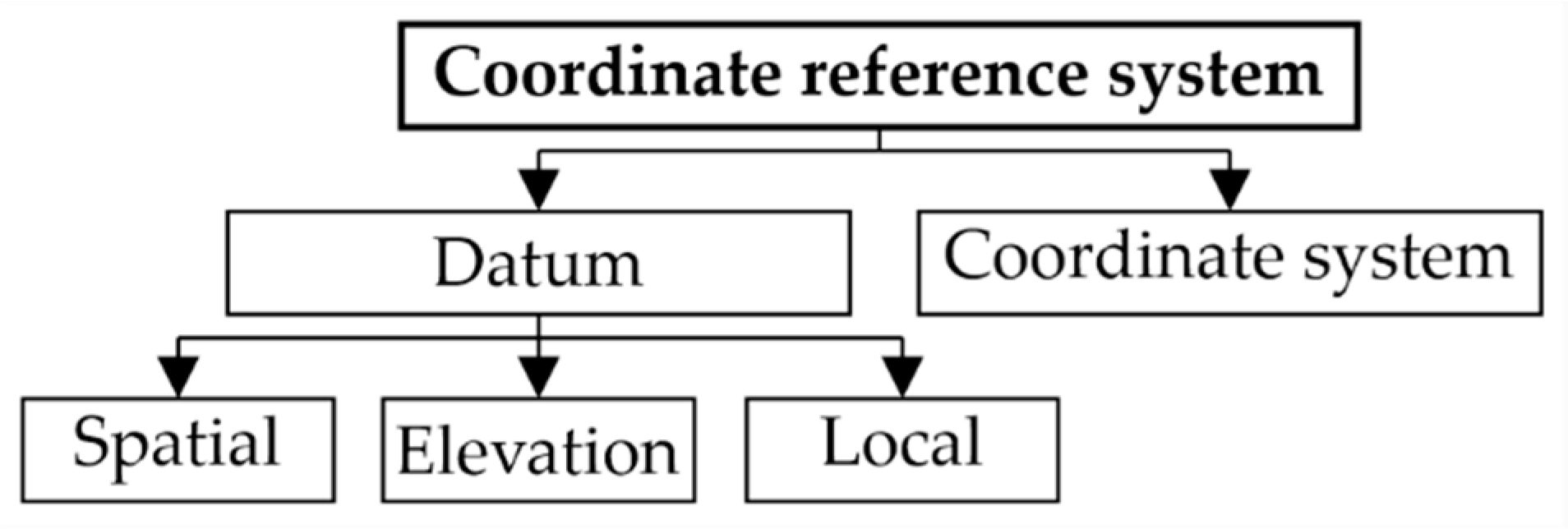
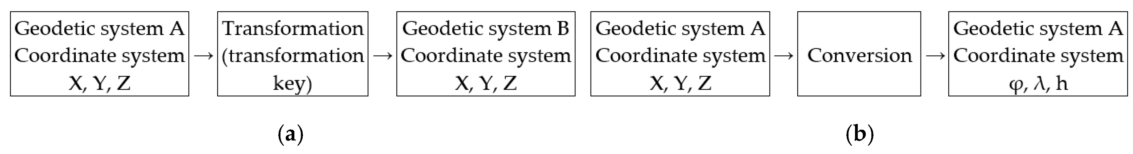
2.3. Transformation of Coordinate Systems
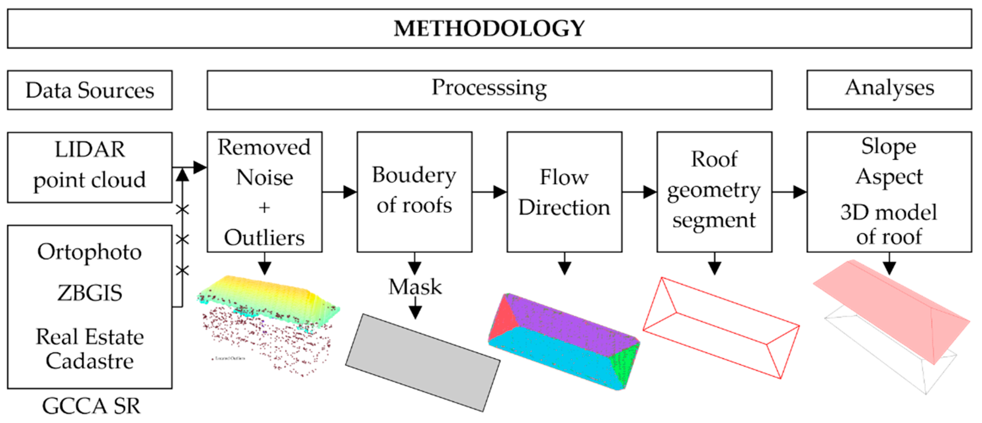
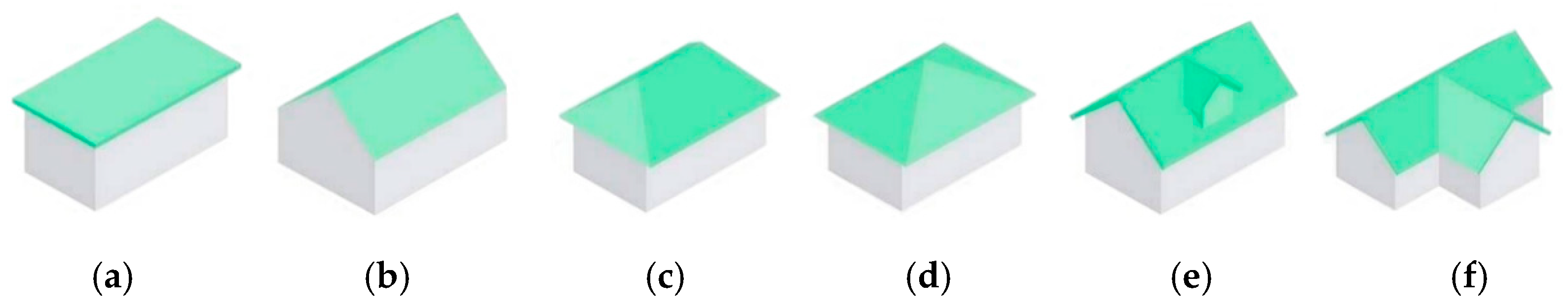
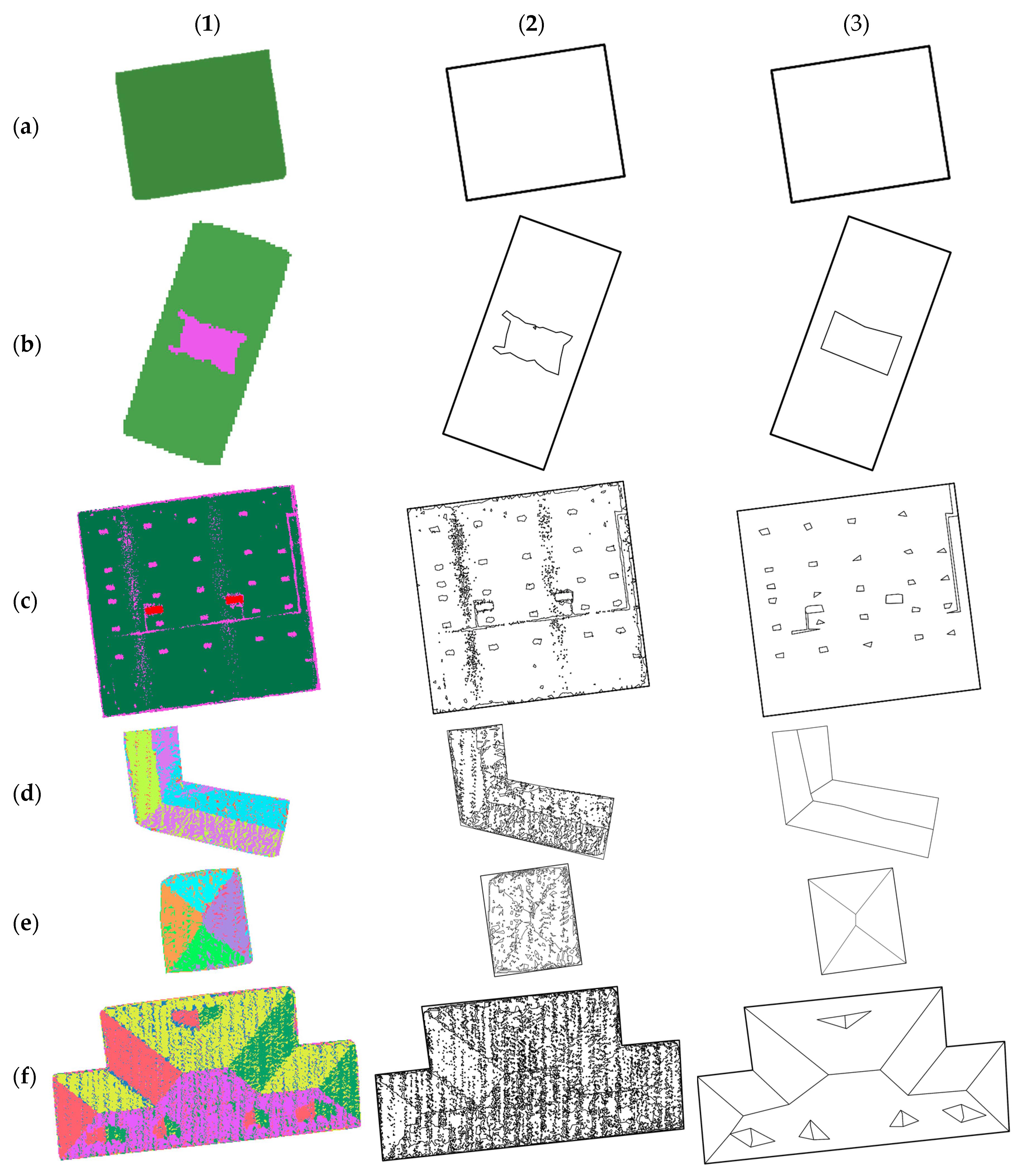
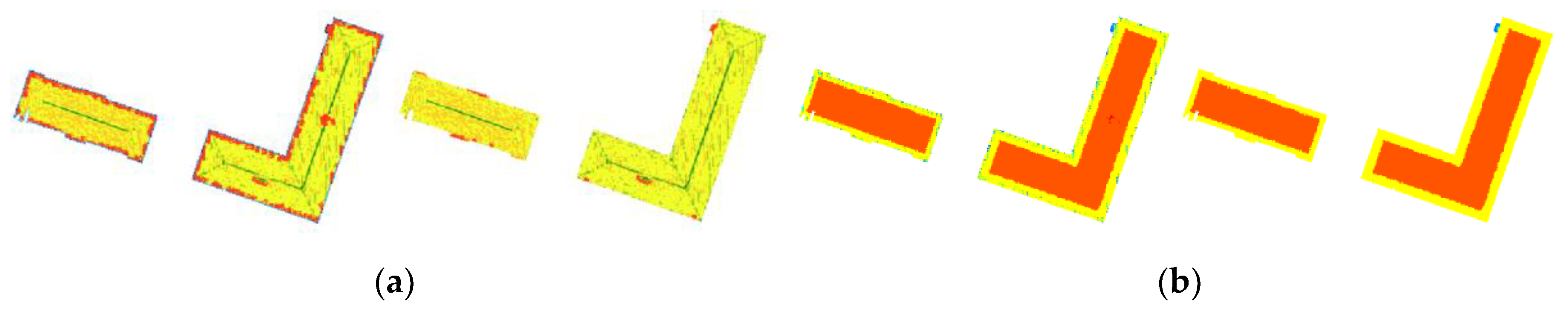
2.4. Detection, Segmentation, and Extraction of Roof Objects
- a minimum area of the roof segment;
- preserving the squareness of the edges of objects (90°);
- the boundary of the roof is made of a fully enclosed polygon without unnecessary holes (gaps).
3. Results and Discussion
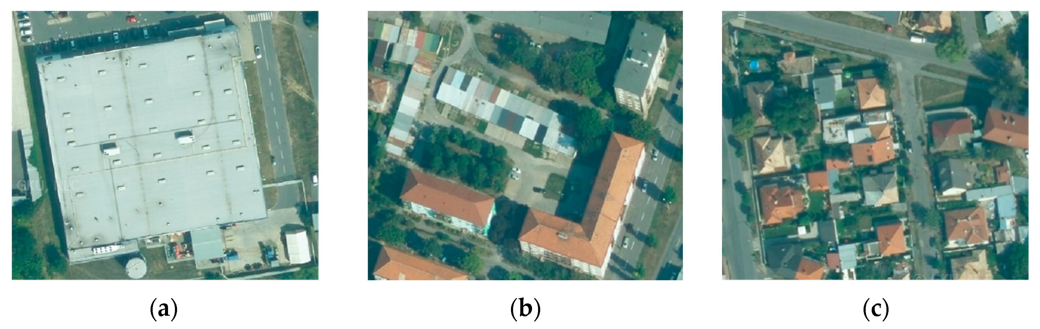
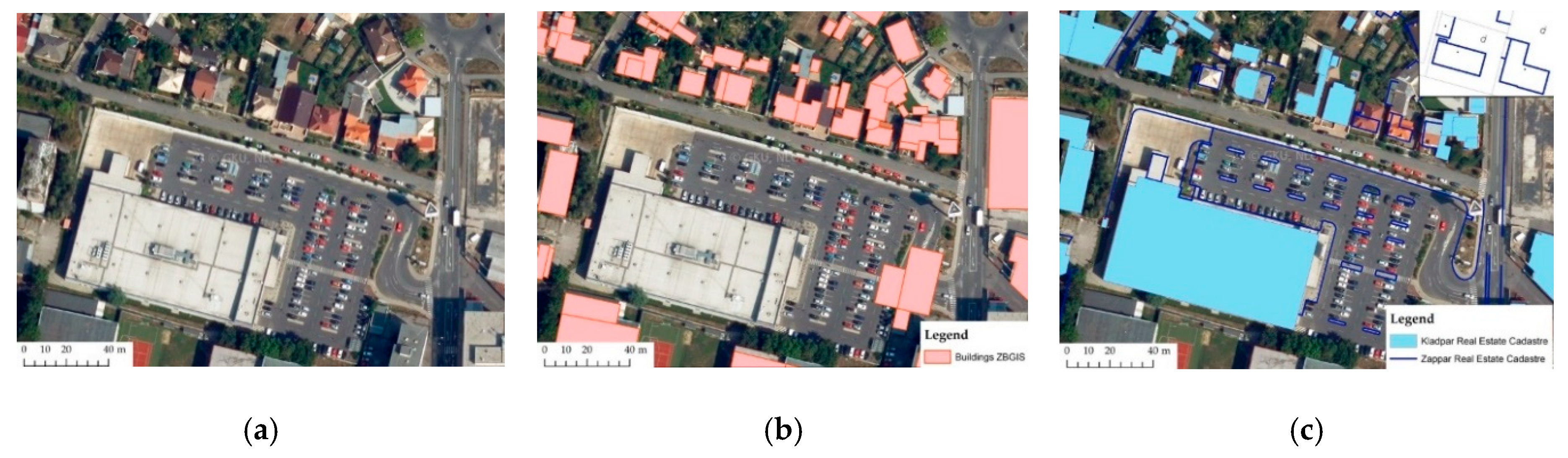
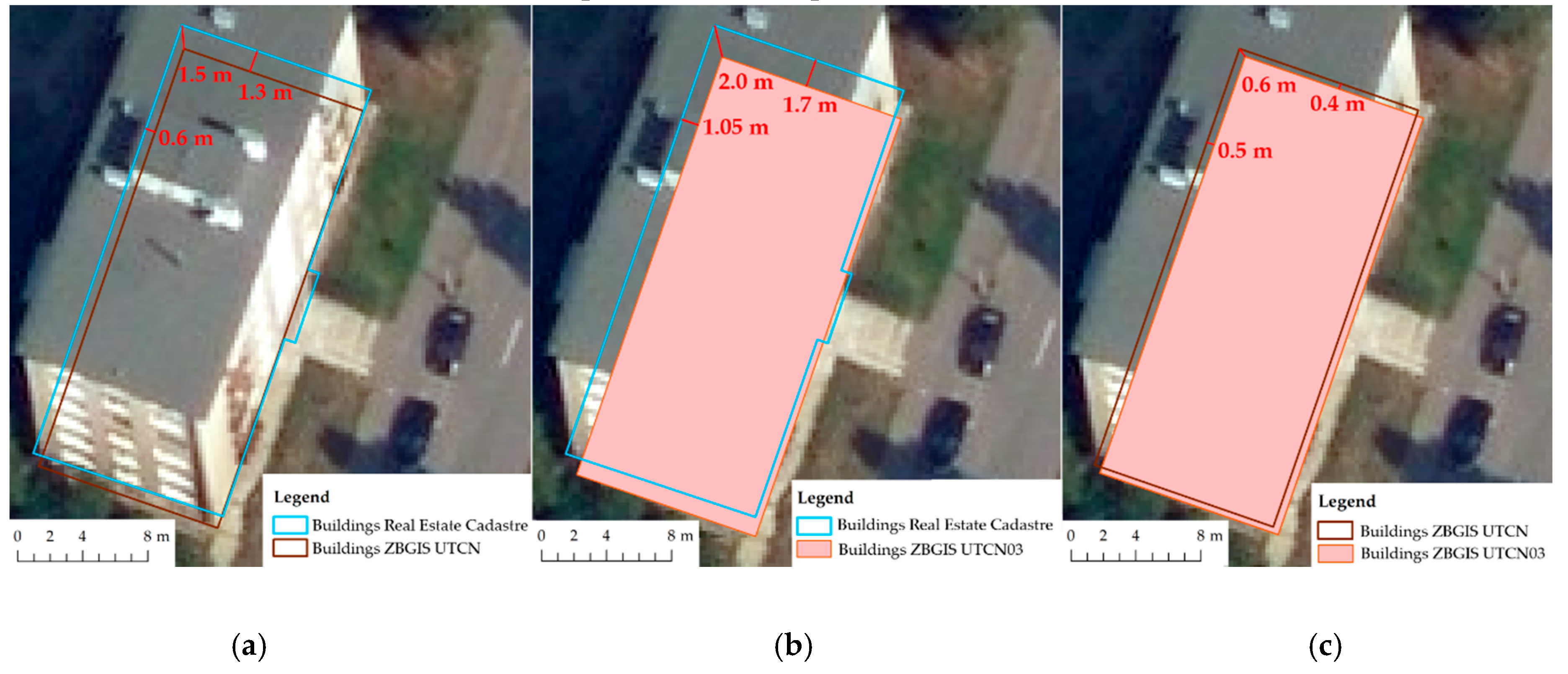
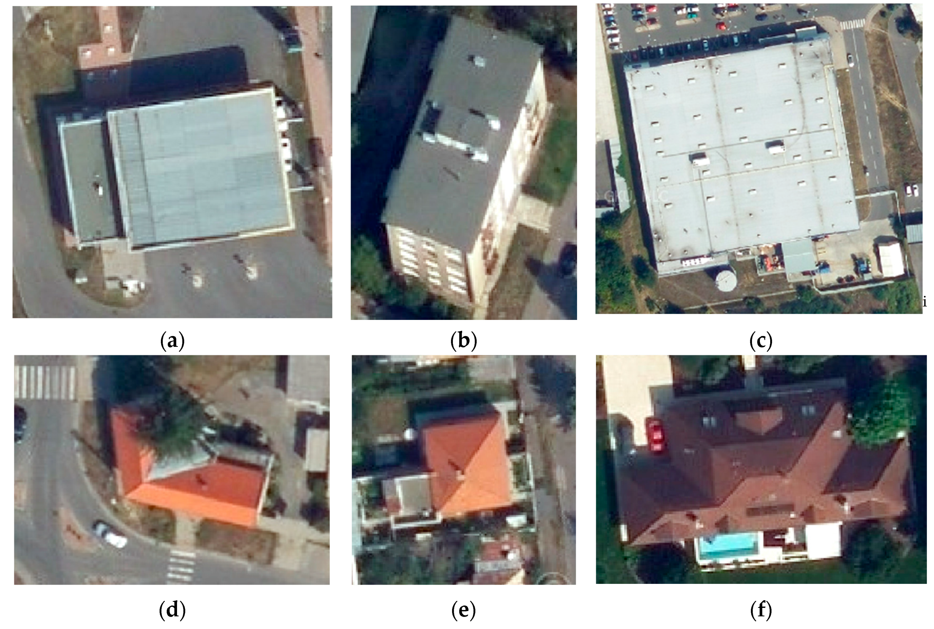
3.1. Comparison of Dataset Integrity from Available National Spatial Databases
- Real Estate Cadastre–Buildings D-UTCN/UTCN;
- ZBGIS–Buildings D-UTCN/UTCN-UTCN03;
- Orthophoto mosaic D-UTCN/UTCN03.
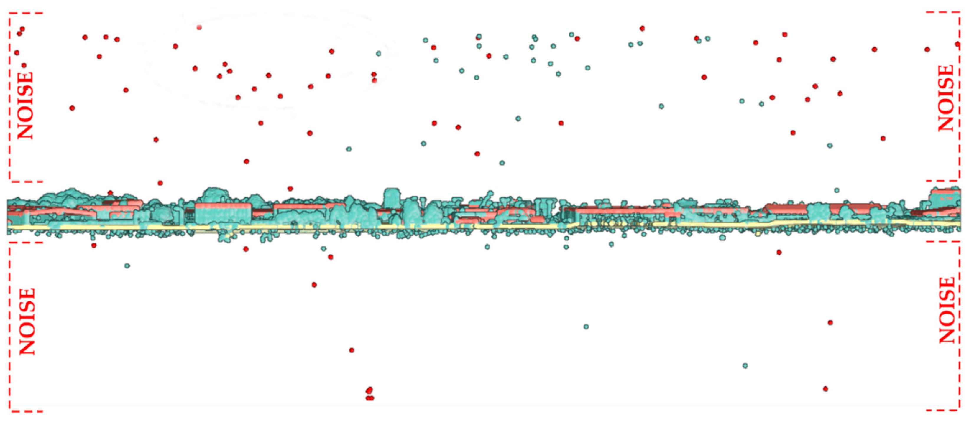
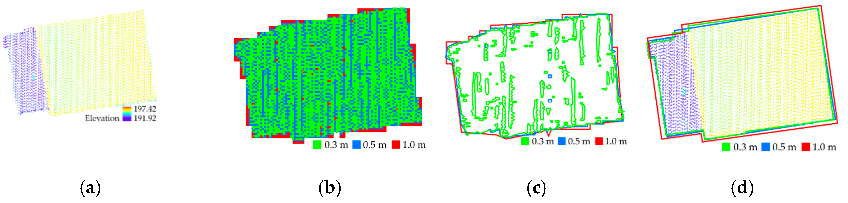
3.2. Input Data Processing—LiDAR Point Cloud
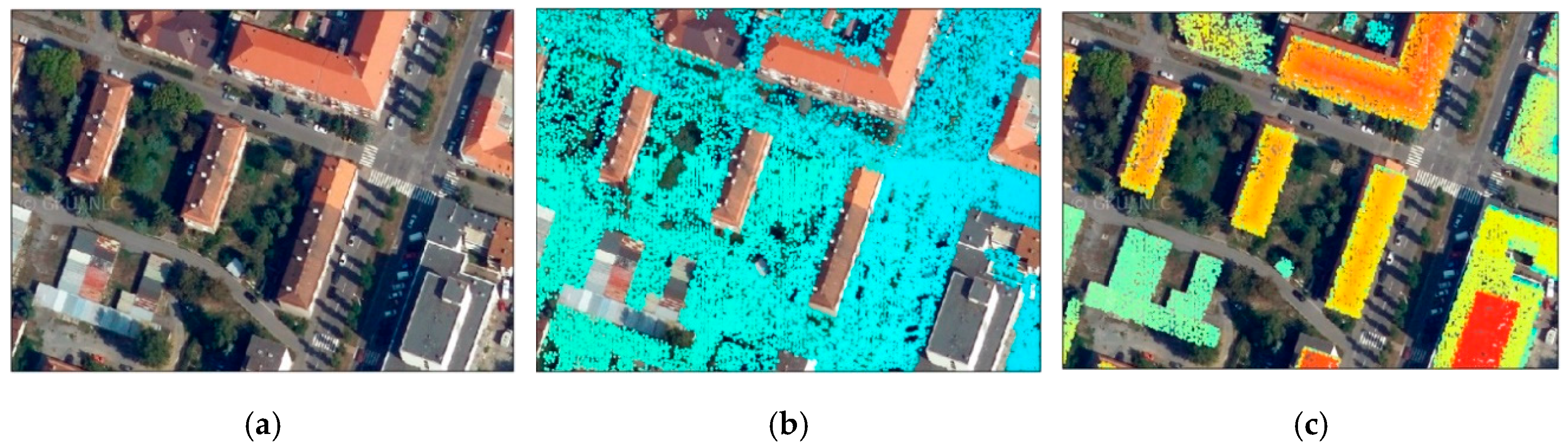
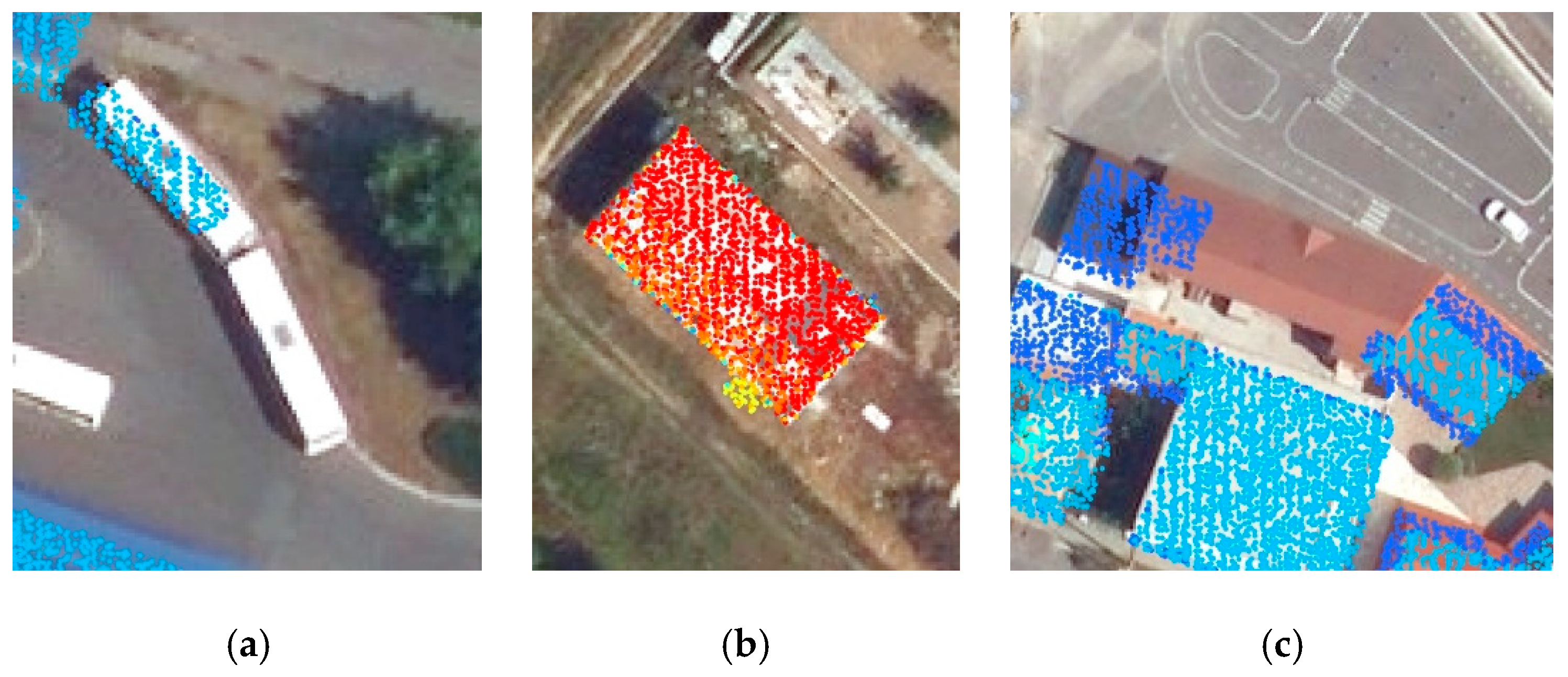
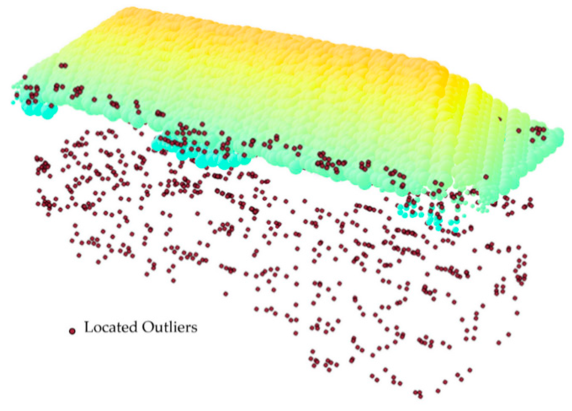
3.3. Detection, Segmentation, and Extraction of Roof Objects
4. Conclusions
Author Contributions
Funding
Conflicts of Interest
References
- Directorate General for Regional Policy, European Commission. Cities of Tomorrow—Challenges, Visions, Ways Forward; European Union: Luxembourg, 2011. [Google Scholar] [CrossRef]
- Al-Bilbisi, H. Spatial Monitoring of Urban Expansion Using Satellite Remote Sensing Images: A Case Study of Amman City, Jordan. Sustainability 2019, 11, 2260. [Google Scholar] [CrossRef] [Green Version]
- Liu, T.; Yang, X. Monitoring land changes in an urban area using satellite imagery, GIS and landscape metrics. Appl. Geogr. 2015, 56, 42–54. [Google Scholar] [CrossRef]
- Diaz-Pacheco, J.; Gutiérrez, J. Exploring the limitations of CORINE Land Cover for monitoring urban land-use dynamics in metropolitan areas. J. Land Use Sci. 2014, 9, 243–259. [Google Scholar] [CrossRef]
- Ovejero-Campos, A.; Fernández, E.; Ramos, L.; Bento, R.; Méndez-Martínez, G. Methodological limitations of CLC to assess land cover changes in coastal environments. J. Coast. Conserv. 2019, 23, 657–673. [Google Scholar] [CrossRef]
- Becker, T.; Nagel, C.; Kolbe, T.H. Semantic 3D modeling of multi-utility networks in cities for analysis and 3D visualization. In Progress and New Trends in 3D Geoinformation Sciences. Lecture Notes in Geoinformation and Cartography; Pouliot, J., Daniel, S., Hubert, F., Zamyadi, A., Eds.; Springer: Berlin/Heidelberg, Germany, 2013. [Google Scholar]
- Kutzner, T.; Hijazi, I.; Kolbe, T.H. Semantic Modelling of 3D Multi-Utility Networks for Urban Analyses and Simulations. Int. J. 3-D Inf. Model. 2018, 7, 1–34. [Google Scholar] [CrossRef] [Green Version]
- Billen, R.; Cutting-Decelle, A.-F.; Marina, O.; de Almeida, J.-P.; Matteo, C.; Falquet, G.; Leduc, T.; Métral, C.; Moreau, G.; Perret, J.; et al. 3D City Models and Urban Information: Current Issues and Perspectives; Edpsciences: Les Ulis, France, 2014. [Google Scholar]
- Biljecki, F.; Stoter, J.; Ledoux, H.; Zlatanova, S.; Çöltekin, A. Applications of 3D city models: State of the art review. ISPRS Int. J. Geo-Inf. 2015, 4, 2842–2889. [Google Scholar] [CrossRef] [Green Version]
- Brito, M.C.; Redweik, P.; Catita, C.; Freitas, S.; Santos, M. 3D solar potential in the urban environment: A case study in lisbon. Energies 2019, 12, 3457. [Google Scholar] [CrossRef] [Green Version]
- Machete, R.; Falcão, A.P.; Gomes, M.G.; Moret Rodrigues, A. The use of 3D GIS to analyze the influence of urban context on buildings’ solar energy potential. Energy Build. 2018, 177, 290–302. [Google Scholar] [CrossRef]
- Santos, T.; Tenedório, J.A.; Gonçalves, J.A. Quantifying the city’s green area potential gain using remote sensing data. Sustainability 2016, 8, 1247. [Google Scholar] [CrossRef] [Green Version]
- Grunwald, L.; Heusinger, J.; Weber, S. A GIS-based mapping methodology of urban green roof ecosystem services applied to a Central European city. Urban For. Urban Green. 2017, 22, 54–63. [Google Scholar] [CrossRef]
- Riffat, S.; Powell, R.; Aydin, D. Future cities and environmental sustainability. Futur. Cities Environ. 2016, 2, 1. [Google Scholar] [CrossRef]
- Haarstad, H.; Wathne, M.W. Are smart city projects catalyzing urban energy sustainability? Energy Policy 2019, 129, 918–925. [Google Scholar] [CrossRef]
- Dornaika, F.; Moujahid, A.; El Merabet, Y.; Ruichek, Y. Building detection from orthophotos using a machine learning approach: An empirical study on image segmentation and descriptors. Expert Syst. Appl. 2016, 58, 130–142. [Google Scholar] [CrossRef]
- Malof, J.M.; Bradbury, K.; Collins, L.M.; Newell, R.G. Automatic detection of solar photovoltaic arrays in high resolution aerial imagery. Appl. Energy 2016, 183, 229–240. [Google Scholar] [CrossRef] [Green Version]
- Gamba, P.; Houshmand, B.; Saccani, M. Detection and extraction of buildings from interferometric SAR data. IEEE Trans. Geosci. Remote Sens. 2000, 38, 611–617. [Google Scholar] [CrossRef] [Green Version]
- Verma, V.; Kumar, R.; Hsu, S. 3D building detection and modeling from aerial LIDAR data. In Proceedings of the IEEE Computer Society Conference on Computer Vision and Pattern Recognition (CVPR’06), New York, NY, USA, 17–22 June 2006. [Google Scholar]
- Ramiya, A.M.; Nidamanuri, R.R.; Krishnan, R. Segmentation based building detection approach from LiDAR point cloud. Egypt. J. Remote Sens. Space Sci. 2017, 20, 71–77. [Google Scholar] [CrossRef] [Green Version]
- Awrangjeb, M.; Ravanbakhsh, M.; Fraser, C.S. Automatic detection of residential buildings using LIDAR data and multispectral imagery. ISPRS J. Photogramm. Remote Sens. 2010, 65, 457–467. [Google Scholar] [CrossRef] [Green Version]
- Demir, N.; Poli, D.; Baltsavias, E. Extraction of Buildings using Images & Lidar Data and a Combination of Various Methods. Int. Arch. Photogramm. Remote Sens. Spat. Inf. Sci. 2009, XXXVIII, 71–76. [Google Scholar] [CrossRef]
- Vu, T.T.; Yamazaki, F.; Matsuoka, M. Multi-scale solution for building extraction from LiDAR and image data. Int. J. Appl. Earth Obs. Geoinf. 2009, 11, 281–289. [Google Scholar] [CrossRef]
- Peng, J.; Zhang, D.; Liu, Y. An improved snake model for building detection from urban aerial images. Pattern Recognit. Lett. 2005, 26, 587–595. [Google Scholar] [CrossRef]
- Kabolizade, M.; Ebadi, H.; Ahmadi, S. An improved snake model for automatic extraction of buildings from urban aerial images and LiDAR data. Comput. Environ. Urban Syst. 2010, 34, 435–441. [Google Scholar] [CrossRef]
- Zhao, C.G.; Zhuang, T.G. A hybrid boundary detection algorithm based on watershed and snake. Pattern Recognit. Lett. 2005, 26, 1256–1265. [Google Scholar] [CrossRef]
- Lou, S.; Pagani, L.; Zeng, W.; Jiang, X.; Scott, P.J. Watershed segmentation of topographical features on freeform surfaces and its application to additively manufactured surfaces. Precis. Eng. 2020, 63, 177–186. [Google Scholar] [CrossRef]
- Zhang, H.; Tang, Z.; Xie, Y.; Gao, X.; Chen, Q. A watershed segmentation algorithm based on an optimal marker for bubble size measurement. Measurement 2019, 138, 182–193. [Google Scholar] [CrossRef]
- Osma-Ruiz, V.; Godino-Llorente, J.I.; Sáenz-Lechón, N.; Gómez-Vilda, P. An improved watershed algorithm based on efficient computation of shortest paths. Pattern Recognit. 2007, 40, 1078–1090. [Google Scholar] [CrossRef]
- Lux, F.; Matula, P. DIC image segmentation of dense cell populations by combining deep learning and watershed. In Proceedings of the 2019 IEEE 16th International Symposium on Biomedical Imaging (ISBI 2019), Venice, Italy, 8–11 April 2019. [Google Scholar]
- Zhang, J.X.; Lin, X.G. Object-based classification of urban airborne lidar point clouds with multiple echoes using SVM. ISPRS Ann. Photogramm. Remote Sens. Spatial Inf. Sci. 2012, I-3, 135–140. [Google Scholar] [CrossRef] [Green Version]
- Kim, A.M.; Olsen, R.C.; Kruse, F.A. Methods for LiDAR point cloud classification using local neighborhood statistics. In Proceedings of the Laser Radar Technology and Applications XVIII, Baltimore, MD, USA, 29 April–3 May 2013. [Google Scholar]
- Zhao, Z.; Cheng, Y.; Shi, X.; Qin, X. Classification method of LiDAR point cloud based on threedimensional convolutional neural network. J. Phys. Conf. Ser. 2019, 1168, 062013. [Google Scholar] [CrossRef]
- Wang, A.; Wang, M.; Wu, H.; Jiang, K.; Iwahori, Y. A novel LiDAR data classification algorithm combined capsnet with resnet. Sensors 2020, 20, 1151. [Google Scholar] [CrossRef] [Green Version]
- Meng, X.; Currit, N.; Zhao, K. Ground filtering algorithms for airborne LiDAR data: A review of critical issues. Remote Sens. 2010, 2, 833–860. [Google Scholar] [CrossRef] [Green Version]
- Huang, R.; Yang, B.; Liang, F.; Dai, W.; Li, J.; Tian, M.; Xu, W. A top-down strategy for buildings extraction from complex urban scenes using airborne LiDAR point clouds. Infrared Phys. Technol. 2018, 92, 203–218. [Google Scholar] [CrossRef]
- Kim, C.; Habib, A. Object-based integration of photogrammetric and LiDAR data for automated generation of complex polyhedral building models. Sensors 2009, 9, 5679–5701. [Google Scholar] [CrossRef] [PubMed]
- Awrangjeb, M. Using point cloud data to identify, trace, and regularize the outlines of buildings. Int. J. Remote Sens. 2016, 37, 551–579. [Google Scholar] [CrossRef]
- Maltezos, E.; Ioannidis, C. Automatic extraction of building roof planes from airborne lidar data applying an extended 3d randomized Hough transform. ISPRS Ann. Photogramm. Remote Sens. Spat. Inf. Sci. 2016, 3, 209–216. [Google Scholar] [CrossRef]
- Höfle, B.; Mücke, W.; Dutter, M.; Rutzinger, M.; Dorninger, P. Detection of Building Regions Using Airborne Lidar–A New Combination of Raster and Point Cloud Based GIS Methods. In Proceedings of the GI_Forum 2009: International Conference on Applied Geoinformatics, Salzburg, Austria, 7 July 2009; pp. 66–75. [Google Scholar]
- Zhang, C.; He, Y.; Fraser, C.S. Spectral Clustering of Straight-Line Segments for Roof Plane Extraction from Airborne LiDAR Point Clouds. IEEE Geosci. Remote Sens. Lett. 2018, 15, 267–271. [Google Scholar] [CrossRef]
- Dos Santos, R.C.; Galo, M.; Carrilho, A.C. Extraction of Building Roof Boundaries from LiDAR Data Using an Adaptive Alpha-Shape Algorithm. IEEE Geosci. Remote Sens. Lett. 2019, 16, 1289–1293. [Google Scholar] [CrossRef]
- El Merabet, Y.; Meurie, C.; Ruichek, Y.; Sbihi, A.; Touahni, R. Building roof segmentation from aerial images using a line-and region-based watershed segmentation technique. Sensors 2015, 15, 3172–3203. [Google Scholar] [CrossRef] [PubMed]
- Slovenský Hydrometeorologický Ústav. Climate Atlas of Slovakia; Slovenský Hydrometeorologický Ústav: Bratislava, Slovakia, 2015; ISBN 978-80-88907-91-6. [Google Scholar]
- Redweik, P.; Catita, C.; Brito, M. Solar energy potential on roofs and facades in an urban landscape. Sol. Energy 2013, 97, 332–341. [Google Scholar] [CrossRef]
- Le, T.B.; Kholdi, D.; Xie, H.; Dong, B.; Vega, R.E. LiDAR-based solar mapping for distributed solar plant design and grid integration in San Antonio, Texas. Remote Sens. 2016, 8, 247. [Google Scholar] [CrossRef] [Green Version]
- Yu, B.; Liu, H.; Wu, J.; Hu, Y.; Zhang, L. Automated derivation of urban building density information using airborne LiDAR data and object-based method. Landsc. Urban Plan. 2010, 98, 210–219. [Google Scholar] [CrossRef]
- Triglav Čekada, M.; Crosilla, F.; Kosmatin Fras, M. Theoretical lidar point density for topographic mapping in the largest scales. Geod. Vestn. 2010, 54. [Google Scholar] [CrossRef]
- Droščák, B. Súradnicový Systém Jednotnej Trigonometrickej Siete Katastrálnej a jeho vzťah k Európskemu Terestrickému Referenčnému Systému 1989. Available online: https://www.geoportal.sk/files/gz/etrs89_s-jtsk_tech_sprava_2014_ver3_0.pdf (accessed on 5 March 2020).
- Demir, N. Automated Detection of 3D Roof Planes from Lidar Data. J. Indian Soc. Remote Sens. 2018, 46, 1265–1272. [Google Scholar] [CrossRef]
- Palmer, D.; Koumpli, E.; Cole, I.; Gottschalg, R.; Betts, T. A GIS-based method for identification of wide area rooftop suitability for minimum size PV systems using LiDAR data and photogrammetry. Energies 2018, 11, 3506. [Google Scholar] [CrossRef] [Green Version]
- Margolis, R.; Gagnon, P.; Melius, J.; Phillips, C.; Elmore, R. Using GIS-based methods and lidar data to estimate rooftop solar technical potential in US cities. Environ. Res. Lett. 2017, 12, 074013. [Google Scholar] [CrossRef]
- Widyaningrum, E.; Gorte, B.; Lindenbergh, R. Automatic building outline extraction from ALS point clouds by ordered points aided hough transform. Remote Sens. 2019, 11, 1727. [Google Scholar] [CrossRef] [Green Version]
- O’Callaghan, J.F.; Mark, D.M. The extraction of drainage networks from digital elevation data. Comput. Vision Graph. Image Process. 1984, 28, 323–344. [Google Scholar] [CrossRef]
- Qin, C.; Zhu, A.X.; Pei, T.; Li, B.; Zhou, C.; Yang, L. An adaptive approach to selecting a flow-partition exponent for a multiple-flow-direction algorithm. Int. J. Geogr. Inf. Sci. 2007, 21, 443–458. [Google Scholar] [CrossRef]
- Tarboton, D.G. A new method for the determination of flow directions and upslope areas in grid digital elevation models. Water Resour. Res. 1997, 33, 309–319. [Google Scholar] [CrossRef] [Green Version]
- Lukač, N.; Seme, S.; Žlaus, D.; Štumberger, G.; Žalik, B. Buildings roofs photovoltaic potential assessment based on LiDAR (Light Detection And Ranging) data. Energy 2014, 66, 598–609. [Google Scholar] [CrossRef]
- Polat, N.; Uysal, M.; Toprak, A.S. An investigation of DEM generation process based on LiDAR data filtering, decimation, and interpolation methods for an urban area. Meas. J. Int. Meas. Confed. 2015, 75, 50–56. [Google Scholar] [CrossRef]
- Lloyd, C.D.; Atkinson, P.M. Deriving DSMs from LiDAR data with kriging. Int. J. Remote Sens. 2002, 23, 2519–2524. [Google Scholar] [CrossRef]
- Shan, W.; Tamura, Y.; Yang, Q.; Li, B. Effects of curved slopes, high ridges and double eaves on wind pressures on traditional Chinese hip roofs. J. Wind Eng. Ind. Aerodyn. 2018, 183, 68–87. [Google Scholar] [CrossRef]
- Lingfors, D.; Bright, J.M.; Engerer, N.A.; Ahlberg, J.; Killinger, S.; Widén, J. Comparing the capability of low- and high-resolution LiDAR data with application to solar resource assessment, roof type classification and shading analysis. Appl. Energy 2017, 205, 1216–1230. [Google Scholar] [CrossRef]
- Martín-Jiménez, J.; Del Pozo, S.; Sánchez-Aparicio, M.; Lagüela, S. Multi-scale roof characterization from LiDAR data and aerial orthoimagery: Automatic computation of building photovoltaic capacity. Autom. Constr. 2020, 109, 102965. [Google Scholar] [CrossRef]
- Matei, B.C.; Sawhney, H.S.; Samarasekera, S.; Kim, J.; Kumar, R. Building segmentation for densely built urban regions using aerial LIDAR data. In Proceedings of the 2008 IEEE Conference on Computer Vision and Pattern Recognition, Anchorage, AK, USA, 23–28 June 2008. [Google Scholar]
- Grêt-Regamey, A.; Celio, E.; Klein, T.M.; Wissen Hayek, U. Understanding ecosystem services trade-offs with interactive procedural modeling for sustainable urban planning. Landsc. Urban Plan. 2013, 109, 107–116. [Google Scholar] [CrossRef]
- Adeleke, A.K.; Smit, J.L. Building roof extraction as data for suitability analysis. Appl. Geomatics 2020. [Google Scholar] [CrossRef]


| Dataset | Release Date | Format | Characteristic |
|---|---|---|---|
| Orthophoto mosaic 1 (Central part of the Slovakia) | 2018 | *.tiff *.tfw | Resolution: 25 cm/pixel Number of channels: 3 (RGB, 8-bit) Coordinate system: D-UTCN (UTCN), code EPSG: 5514 Accuracy: RMSExy = 0.30 m CE90 = 1.5175 × RMSExy = 0.45 m CE95 = 1.7308 × RMSExy = 0.52 m |
| LiDAR 1 point cloud | XI. 2018 –IV. 2019 | *.las | An altitude accuracy of cloud points: 0.03 m A position accuracy of cloud points: 0.11 m The average density of points (last reflection): 19 pt/m2 Coordinate system: D-UTCN (UTCN03) |
| Buildings ZBGIS 1 | 2005–2018 | *.shp | Attribute table FACC (DIGEST code) Objects update date = 2005–2018 horizontal and vertical accuracy code: 1 = Geodetic (<0.1 m) 2 = Photogrammetric (<1 m) 3 = Photogrammetric (<5 m) 4 = Photogrammetric on relief (<1 m) 997 = Estimated height (>5 m) Coordinate system: D-UTCN (UTCN), EPSG code: 5514 |
| Buildings–Real Estate Cadastre 1 | VI.2020 | *.shp *.vgi | The set of geodetic information Vector cadastral map Coordinate system: D-UTCN (UTCN), EPSG code: 5513 |
| Geodetic Reference System | Code | Implementation of the Geodetic Reference System | Code | EPSG Code |
|---|---|---|---|---|
| European Terrestrial Reference System 1989 | ETRS89 | Slovak Terrestrial Reference Framework 2009 | SKTRF09 = ETRF2000 | 4937 (3D-φ, λ, h 4258 (2D-φ, λ) 4936 (3D-X, Y, Z) |
| Datum of Unified Trigonometric Cadastral Network | D-UTCN | Uniform Trigonometric Cadastral Network | UTCN | 2065 (Ferro) 5513 (Greenwich) |
| Uniform Trigonometric Cadastral Network 2003 | UTCN03 | 8352 (Greenwich) | ||
| Baltic Vertical Datum -After Adjustment | BVDaA | Baltic Vertical Datum -After Adjustment | BVDaA (1957) | 8357 |
| The Direction of the Transformation | |||
|---|---|---|---|
| ETRS89 (ETRF2000) → D-UTCN (UTCN03) | D-UTCN (UTCN03) → ETRS89 (ETRF2000) | ||
| The shift in the axis direction | Axis rotation | The shift in the axis direction | Axis rotation |
| TX = −485.014055 m | RX = 7.78625453″ | TX = 485.021 m | RX = −7.786342″ |
| TY = −169.473618 m | RY = 4.39770887″ | TY = 169.465 m | RY = −4.397554″ |
| TZ = −483.842943 m | RZ = 4.10248899″ | TZ = 483.839 m | RZ = −4.102655″ |
| Classification | Absolute Frequency | Relative Frequency |
|---|---|---|
| Unassigned | 1,194,562 | 3.62% |
| Ground | 18,036,417 | 54.62% |
| Low vegetation | 1,882,184 | 5.70% |
| Medium vegetation | 1,240,739 | 3.76% |
| High vegetation | 3,883,862 | 11.76% |
| Buildings | 6,599,697 | 19.99% |
| Noise | 3,888 | 0.01% |
| High noise | 10,808 | 0.03% |
| Water | 167,045 | 0.51% |
| Total number of points | 33,019,202 | 100.00% |
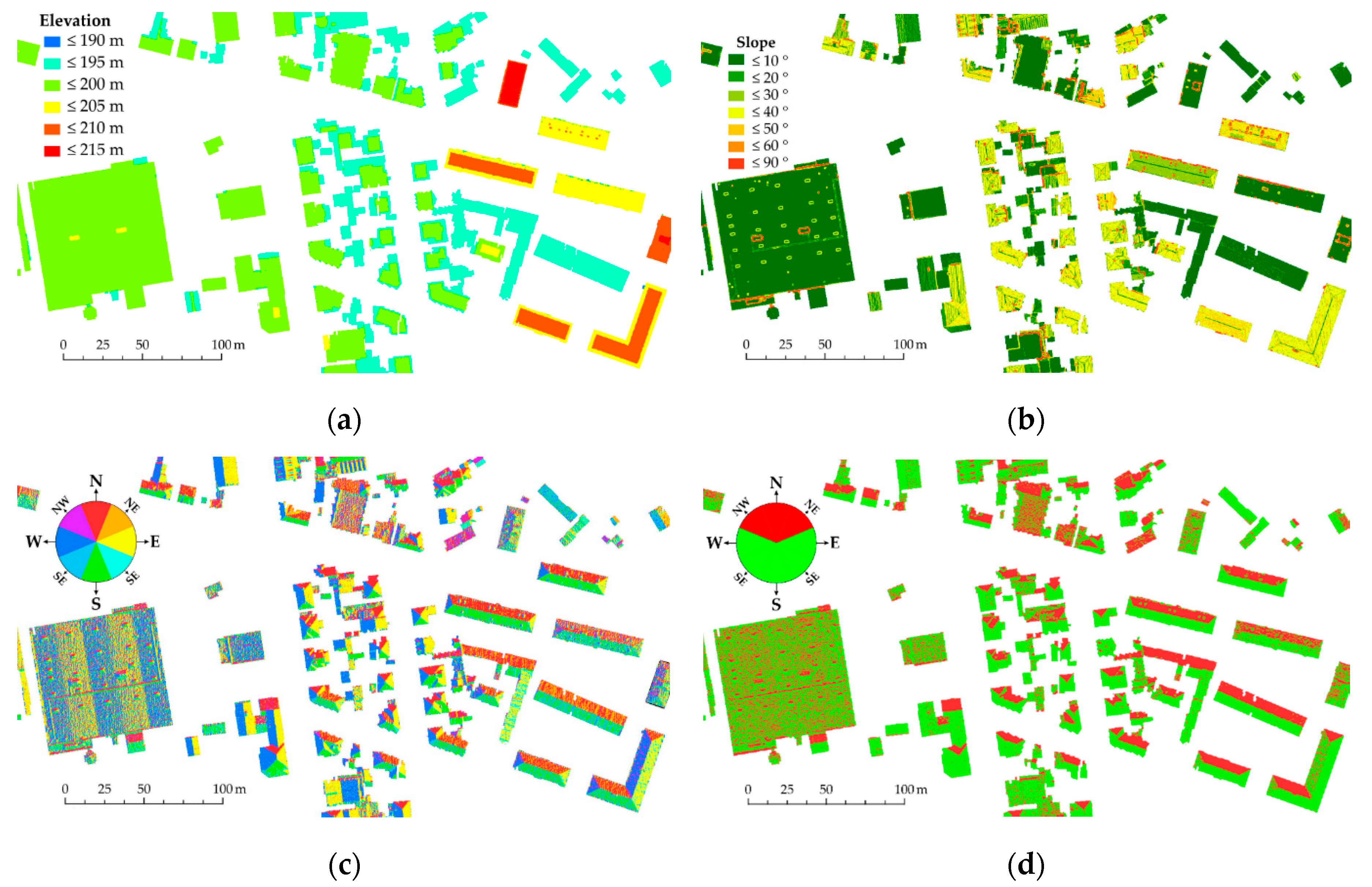
| Slope Value [°] | Classified Value | Roof Categories | Colored Scale |
|---|---|---|---|
| 0–10 | 1 | flat |  |
| 10–20 | 2 | sloping |  |
| 20–30 | 3 | sloping |  |
| 30–40 | 4 | sloping |  |
| 40–50 | 5 | sloping |  |
| 50–60 | 6 | roof objects |  |
| 60–90 | 7 | roof objects |  |
| Azimuth Value [°] | Azimuth Orientation | Classified Value | Colored Scale | Recolored Scale |
|---|---|---|---|---|
| 0–22.5 | North | 1 |  |  |
| 22.5–67.5 | North-east | 2 |  |  |
| 67.5–112.5 | East | 3 |  |  |
| 112.5–157.5 | South-east | 4 |  |  |
| 157.5–202.5 | South | 5 |  |  |
| 202.5–247.5 | South-west | 6 |  |  |
| 247.5–292.5 | West | 7 |  |  |
| 292.5–337.5 | North-west | 8 |  |  |
| 337.5–360... | North | 9 |  |  |
© 2020 by the authors. Licensee MDPI, Basel, Switzerland. This article is an open access article distributed under the terms and conditions of the Creative Commons Attribution (CC BY) license (http://creativecommons.org/licenses/by/4.0/).
Share and Cite
Gergelova, M.B.; Labant, S.; Kuzevic, S.; Kuzevicova, Z.; Pavolova, H. Identification of Roof Surfaces from LiDAR Cloud Points by GIS Tools: A Case Study of Lučenec, Slovakia. Sustainability 2020, 12, 6847. https://0-doi-org.brum.beds.ac.uk/10.3390/su12176847
Gergelova MB, Labant S, Kuzevic S, Kuzevicova Z, Pavolova H. Identification of Roof Surfaces from LiDAR Cloud Points by GIS Tools: A Case Study of Lučenec, Slovakia. Sustainability. 2020; 12(17):6847. https://0-doi-org.brum.beds.ac.uk/10.3390/su12176847
Chicago/Turabian StyleGergelova, Marcela Bindzarova, Slavomir Labant, Stefan Kuzevic, Zofia Kuzevicova, and Henrieta Pavolova. 2020. "Identification of Roof Surfaces from LiDAR Cloud Points by GIS Tools: A Case Study of Lučenec, Slovakia" Sustainability 12, no. 17: 6847. https://0-doi-org.brum.beds.ac.uk/10.3390/su12176847