Prediction of Fuel Loading Following Mastication Treatments in Forest Stands in North Idaho, USA


Forest Operations Research Lab, College of Natural Resources, University of Idaho, 875 Perimeter Drive, Moscow, ID 83844-4264, USA
*
Author to whom correspondence should be addressed.
Sustainability 2020, 12(17), 7025; https://0-doi-org.brum.beds.ac.uk/10.3390/su12177025
Submission received: 7 August 2020
/
Revised: 21 August 2020
/
Accepted: 21 August 2020
/
Published: 28 August 2020
(This article belongs to the Special Issue Technologies, Applications and Assessments for Proper Sustainable Forest Operations (SFO))
Abstract
:Fuel reduction in forests is a high management priority in the western United States and mechanical mastication treatments are implemented common to achieve that goal. However, quantifying post-treatment fuel loading for use in fire behavior modeling to forecast treatment effectiveness is difficult due to the high cost and labor requirements of field sampling methods and high variability in resultant fuel loading within stands after treatment. We evaluated whether pre-treatment LiDAR-derived stand forest characteristics at 20 m × 20 m resolution could be used to predict post-treatment surface fuel loading following mastication. Plot-based destructive sampling was performed immediately following mastication at three stands in the Nez Perce Clearwater National Forest, Idaho, USA, to correlate post-treatment surface fuel loads and characteristics with pre-treatment LiDAR-derived forest metrics, specifically trees per hectare (TPH) and stand density index (SDI). Surface fuel loads measured in the stand post-treatment were consistent with those reported in previous studies. A significant relationship was found between the pre-treatment SDI and total resultant fuel loading (p = 0.0477), though not between TPH and fuel loading (p = 0.0527). SDI may more accurately predict post-treatment fuel loads by accounting for both tree number per unit area and stem size, while trees per hectare alone does not account for variations of tree size and subsequent volume within a stand. Relatively large root-mean-square errors associated with the random forest models for SDI (36%) and TPH (46%) suggest that increased sampling intensity and modified methods that better account for fine spatial variability in fuels resulting from within-stand conditions, treatment prescriptions and machine operators may be needed. Use of LiDAR to predict fuel loading after mastication is a useful approach for managers to understand the efficacy of fuel reduction treatments by providing information that may be helpful for determining areas where treatments can be most beneficial.
1. Introduction
Due to the variability of species, management objectives, spatial configuration of management areas, regulatory restrictions, landowner funding availability, fuels characteristics, and other geographic and vegetative factors, developing a one-size-fits-all approach for wide-scale fire management is challenging [1,2,3,4]. However, forests with high fire risk must be actively managed [5]. Over the previous century, forest management practices such as fire exclusion have resulted in historically uncharacteristic stand attributes in many forests in the western United States, including dense, small-diameter stands with increased surface fuel loads [5,6]. Fuel reduction in stands that have lacked prior density management is a high priority in many areas of the western United States, especially on federal lands. Understanding the unique challenges and selecting strategies to best suit the needs of each management area, typically applied through one or more treatments applied at the stand level, is vital to long-term management success [2]. Properly designed and implemented fuel treatments have been found to increase fire resilience and resistance while simultaneously changing the behavior of wildfires that impact treated areas [5,7,8,9].
Given the variability of management factors, including forest composition, topography, climatic conditions, and management history, not all silvicultural and fuel reduction treatments are feasibly implemented. In its most basic form, creating fire resilient stands generally involves three objectives: reducing surface fuels, reducing ladder fuels, and reducing crown density [5]. The complexity of planning fuel treatments for influencing the behavior of large fires must also account for spatial configuration and density of treatments when determining how to effectively and efficiently treat landscapes [4]. Fuel treatment programs have been implemented across the Western United States and include prescribed burning and mechanical treatments such as regeneration harvest, precommercial and commercial thinning, and mastication. The risk of fire escape, smoke restrictions, and poor public perception may limit the feasibility of large-scale prescribed burning efforts [10]. The need to meet particular site and climatic conditions to successfully implement prescribed burning often results in limited availability of windows in prescription, unlike mechanized treatments, that are less dependent on these factors [2]. To mimic the changes to forest structure created by fire, mechanical treatments are widely used to reduce crown fire risk, particularly in the Wildland Urban Interface (WUI) [10]. Mechanical treatments modify the vertical distribution of fuels and reduce overall canopy fuels to levels that are less susceptible to crown fires and rapid fire spread, without the risks associated with prescribed burning.
In many cases, stands that are at risk for severe fire are overstocked and may have high levels or mortality, which reduces the merchantable stand volume component and reduces the profitability of commercial timber harvest in the context of salvage harvesting. Alternative mechanical fuel treatment options, including mastication and chipping, are used in these instances when revenue from timber harvest may not be a core management objective, but fuel loads nevertheless need to be reduced. In these operations, which occur commonly on federal lands, fuels generated are left on site, unlike final harvest and commercial thinning treatments, where harvested materials are most commonly removed, treated at the landing, or treated in piles within the unit. The size of mechanical fuel treatments is dependent on the overall management objectives of the area. Mastication may target relatively small, high fire risk areas possessing dangerous fuel loads, where harvesting is not feasible. Alternatively, larger mastication operations may be used to reduce canopy density and ladder fuels while simultaneously reducing competition, removing undesirable trees, and preparing the stand for future harvest. Mastication entails the grinding, shredding, chunking, or by other means reducing the size of both standing and downed materials via boom-mounted mulching attachments of excavators, skid-steers, or other machines [11,12,13]. The risk of active crown fires is reduced by altering the vertical distribution and continuity of forest fuels and compacting them on the forest floor as irregularly shaped chips, though dead surface fuel loads are increased in the process [10,14]. Changes in physical properties of woody material resulting from mastication can influence fire behavior, including the rate of spread, flame length, and intensity [14]. According to Agee and Skinner [5], reducing surface fuels, increasing live crown height, retaining large, fire resistant trees, and decreasing crown bulk density are all important factors in producing fire-resistant stands. Altering the amount and condition of ladder fuels similarly influences fire intensity and burn severity [12]. When implemented correctly, mechanized fuel treatments address all points, excluding the reduction of surface fuel.
Despite the widespread use of mastication treatments [15] and past research, the spatial variability of masticated fuel beds has not been previously studied [10,11]. Studies have found surface fuel loadings in mulched treatments to range from 16 to 65 Mg ha−1, with woody fuels concentrated in the 1-h and 10-h time-lag classes, which have average diameters < 2.54 cm [10,14,16,17,18]. Relative to untreated stands, mulched fuel beds with fuels concentrated in these classes have reduced rate of spread and flame lengths, but increased smoldering and flaming duration [10]. Quantifying masticated fuel loads is challenging, however, given the wide variability in masticated fuel physical structures and site, ecosystem, and regional fuel characteristics [15]. In masticated stands, fuel loads are also highly variable, leading to challenges when predicting and modeling loading and fire behavior. Fuel loads rely heavily on multiple factors, including vegetation type, pretreatment stand conditions, machinery and mastication attachment, operator and the treatment objectives, and desired conditions post-treatment [10,14,15,16,17]. As a result, the spatial heterogeneity of fuels within and across masticated stands remains unclear [15]. Several studies have successfully used fuel depth and/or fuel coverage in mulched areas to estimate surface fuel loads [10,14,17,18]. These techniques provide total surface fuel estimates more easily and accurately than planar transect sampling, but still require visiting the site following treatments. While less labor-intensive than past methods, the widespread assessment of surface fuel loading following mastication still requires in-person site visitation and assessment, which can be time-intensive and is only possible post-treatment. Efficient and effective methods to map post-treatment fuel loadings using pre-treatment conditions across stand, site, forest, and broader extents could provide valuable information to landowners when developing fuel management programs and evaluating their potential cost-effectiveness.
Fuel mapping is a difficult and often infeasible process across broad spatial and temporal scales due to high fuel variability, and costs and time constraints associated with field sampling [19,20,21,22]. Given the additional variability of masticated fuel loads, prediction models will likely need to focus on relatively small geographic extents and account for various forest characteristics. Micro-site predictions may better address site and forest variability and result in more accurate models. To better understand fuel loads resulting from treatments, it is important to first determine what forest conditions existed prior to mastication. On large landscape and regional scales, it is infeasible to perform a forest inventory to determine pre-treatment conditions due to labor and cost restrictions. Therefore, remotely sensed data, specifically LiDAR, has been repeatedly shown to provide large-scale forest metric predictions and enable the future extrapolation of models [23]. LiDAR has been used in part or entirely for assessing forest fuels characteristics including canopy [24,25,26], surface fuel loading [27,28,29,30,31], ladder fuels [32,33] and parameters including overall loading, spatial distribution, composition, vertical and horizontal arrangement, bulk density, and hazard ratings [34,35,36,37,38]. The authors were unable to find any relevant studies for LiDAR applications in masticated surface fuel loadings. Additionally, no models have currently been developed to predict post-mastication surface fuel loads from pre-treatment LiDAR-derived stand conditions.
In this study, we evaluate whether pre-treatment LiDAR-derived forest metrics can be used to predict surface fuel loads and associated fuel characteristics following mastication treatments. Masticated fuels were assessed across varying pre-treatment stand conditions to determine if relationships exist between the masticated fuel loads and LiDAR-derived forest metrics prior to treatment. Additionally, relationships between pre-treatment metrics and additional fuel bed characteristics including depth, size class distribution, and bulk density were assessed. Masticated fuels were sorted and quantified based on time-lag classes to determine if pre-treatment stand characteristics impact these distributions within sample plots. If remotely sensed forest metrics relate directly to mastication fuel characteristics, these models could be used to predict fuel loading and fuel bed characteristics for areas of similar forest composition, prior to mastication treatments. This information provides valuable insight to natural resources managers when selecting potential forest and fuel treatment options, ensuring both the economic and ecological sustainability of mechanical fuel treatments and other concurrent forest operations. Economically and ecologically unsustainable fuel treatments are financially and operationally infeasible, unsuccessful in achieving the desired operational, environmental and management results, and lead to the inefficient and ineffective use of limited financial resources. Understanding the potential impacts of mastication treatments based on existing forest conditions will help assess areas where this treatment option can be implemented cost-effectively when—coupled with existing fire behavior models.
2. Materials and Methods
2.1. Study Site
The study sites were located in three stands in the Nez Perce-Clearwater National Forest, in north central Idaho, following fuel treatments to gather data pertaining to the resultant surface fuel loads. These treatments were part of the larger Orogrande timber sale and consisted of approximately 38 hectares (95 acres) of mechanical fuel treatment. The management units were predominantly mixed conifer forest type with slopes averaging 35% throughout the units. Mastication was successfully implemented in the three stands as a management alternative to timber harvest. The three stands treated for this study were originally planned for timber harvest. Harvesting was found to be financially infeasible due to the low value of harvested products and long-haul distances to the mill. The prescription developed for the project was intended to release remaining trees to increase timber value for future harvest while simultaneously decreasing stand density and increasing canopy base height to reduce the risk of crown fire using mastication. According to forest personnel, the management approach used in this project was its first application on the Nez Perce-Clearwater National Forest. The machine used to perform the mechanical fuel treatment was a Takeuchi TB290 compact excavator with a Fecon Bull Hog mastication head (Figure 1). The machine weighs 8685 kg, is 2.2 m wide and 2.9 m long at the undercarriage, has a maximum reach of 7.4 m, and creates only 37.9 kPa of ground pressure when equipped with 450-mm-wide rubber tracks.
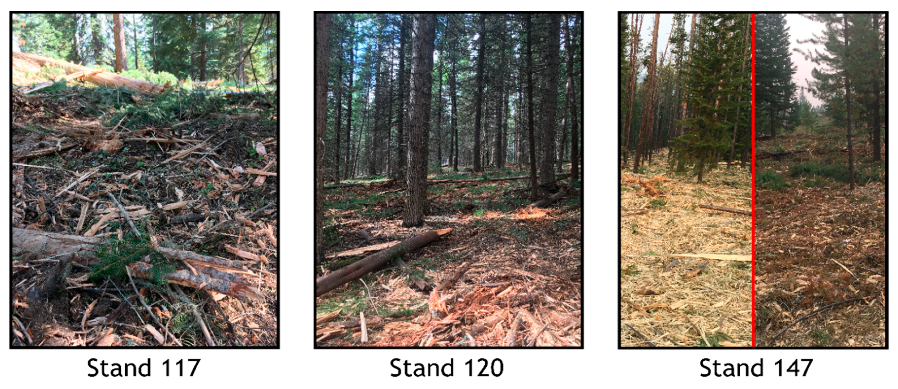
The treatment prescription for the stands included a target range for post-treatment stocking level. For the units in this study, the operator was instructed to leave 40 to 80 trees per hectare after treatment while removing only stems less than 18 cm (7 inches) in diameter. Further, all dead and down material up to 30 cm (12 inches) were masticated [39]. Post-treatment surface fuel sampling occurred in the masticated portions of three replicate stands: 117 (13 hectares), 120 (15 hectares), and 147 (10 hectares), within the management boundary. Due to many downed trees in stand 147, meeting the prescription specification for dead and downed material was not operationally feasible. Therefore, the mastication intensity for downed trees was reduced after stand 147 was partially treated. This prescription adjustment was used for treating the remainder of stand 147 and for the entirety of stands 117 and 120 [39] (Figure 2).
2.2. LiDAR Processing and Sample Plot Selection
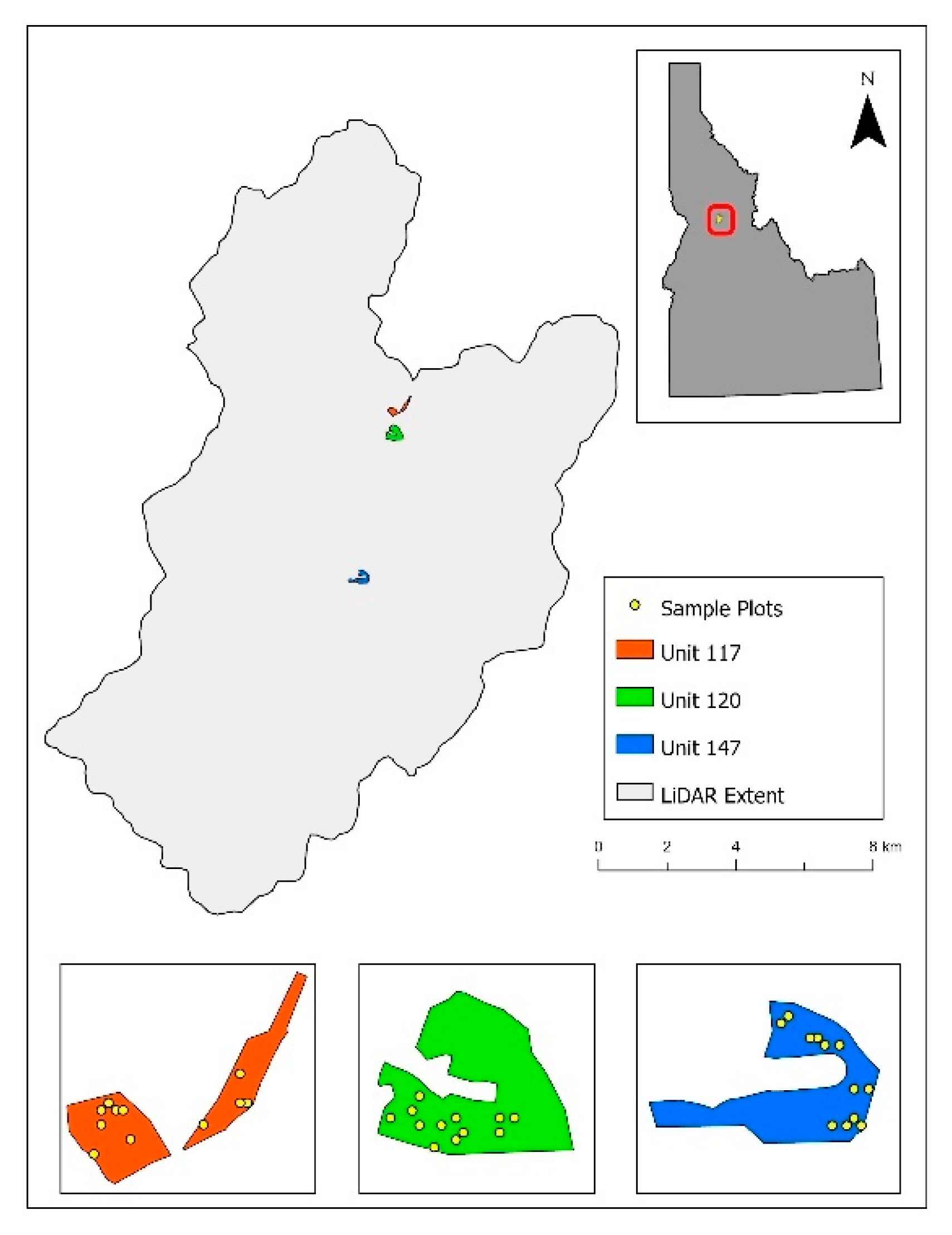
The Orogrande timber sale and the three stands (117, 120, 147) were within the extent of the 18,450-hectare (45,600-acre) Crooked River LiDAR acquisition flown in 2012 with a pulse density return of ≥4 points per square meter (Figure 3). Field sampling inventory data from 91 20 × 20-m (1/10 acre) plots were run through the USFS Forest Vegetation Simulator [40] to summarize stand composition and structure. These forest inventory data were part of a previous sampling effort and were collected using field methods described in Falkowski et al. (2005) [22]. Random forest models [41,42] describing trees per hectare, total volume (m3 ha−1), basal area (m2 ha−1), and stand density index (SDI) were then developed using LiDAR metrics encompassing identical extents to the field sampling plots. These methods are consistent with those described in Becker et al. [43]. All random forest development and metric predictions were performed in the open source statistical analysis program, R, using the randomForest package [42,44].
Random forest ensemble learning algorithms were used because they provide excellent classification results, speed of processing, ability to reduce bias, and correlation and reduce overfitting compared to other classification and regression trees (CART) models, making them a widely used machine learning solution [45,46,47,48]. Random forest produces multiple decision trees using bagging and randomly selected subsets of training samples and variables to provide a majority vote from which a prediction is made. The default number of trees (ntree = 500) and the default number of variables split at each node (mtry = square root of the total number of input variables) were used when building random forest models for each forest characteristic. 177 LiDAR metrics were available to develop each unique random forest algorithm, but only a subset of metrics were used in the final models, based on importance, defined using rfUtilities [49]. Random forest models were built using 2/3 of the data and validated using the remaining 1/3 of the data.
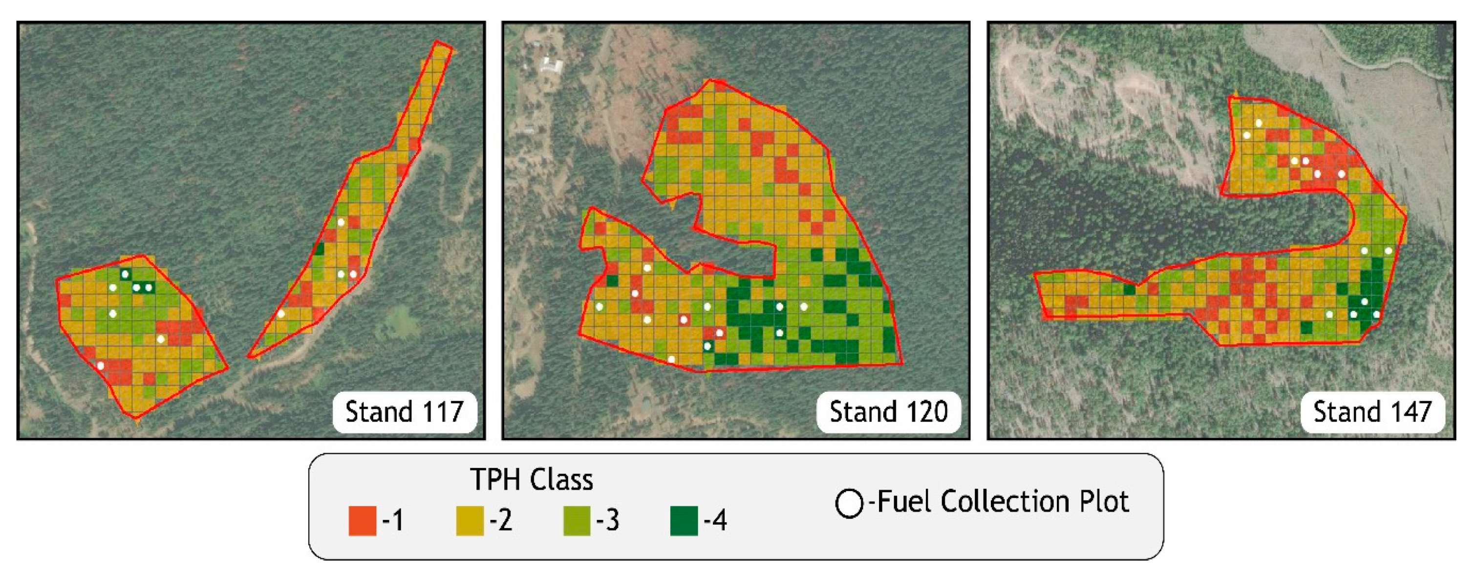
The entire Crooked River LiDAR acquisition was processed using the USDA LiDAR processing software FUSION version 3.60 to create an identical post-processed data structure as the initial 91 sampled plots [50]. This enabled the random forest models to be applied directly to the whole area to develop predicted metrics in 20 × 20-m pixels. Stand metrics derived from the LiDAR analysis included trees per hectare (TPH), total cubic foot volume (m3 ha−1), total basal area (m2 ha−1), and stand density index. SDI has been used in even-aged monocultures, and more recently in uneven-aged, mixed species stands to assess stand density as a function of quadratic mean diameter and stem density [51,52,53,54,55]. This metric was selected in addition to TPH to provide a more descriptive indication of stand density. The trees per hectare vector map was then stratified into four classes: 0–247; 248–494; 495–740; 741+. These classes were used to select sample plots within the study stands. Trees per hectare classes were used to stratify the selection of a broad distribution of relative stocking in sampled areas prior to mastication.
2.3. Field Sampling Procedures
Twelve plots were sampled within each of the three stands, with three representing each of the four levels of pre-treatment trees per hectare derived from the LiDAR data. The 20 × 20-m pixels chosen for sampling were randomly selected from all available pixels of the trees per hectare class within the stand boundaries. The resulting sampled pixels amounted to 36, with nine plots representing each of the four classes of pre-treatment trees per hectare. Trees per hectare was selected as the stand metric by which to select sample plots, due to the mastication treatment prescription being based on a goal trees per hectare post-treatment. All mastication treatments and sampling of fuel loading occurred during summer 2017.
Center points within the 20 × 20-m pixels were determined via ArcMap, and the resultant coordinates were used to locate the field plot centers. A simple method of plot center relocation was established to address situations where plot centers occur in areas that prohibited the sampling of fuel loading including tree stumps, roadways, rock outcroppings, and exposed mineral soil due to machinery movement. In these instances, plot centers were moved due north 3 m. If needed, plots were moved due west from original plot centers 3 m if the movement due north did not resolve the issue with the obstruction. A variation on destructive plot-based sampling was used to quantify fuel characteristics and fuel loading following mastication treatments within the three stands at each of the 36 plots [10,14,17].
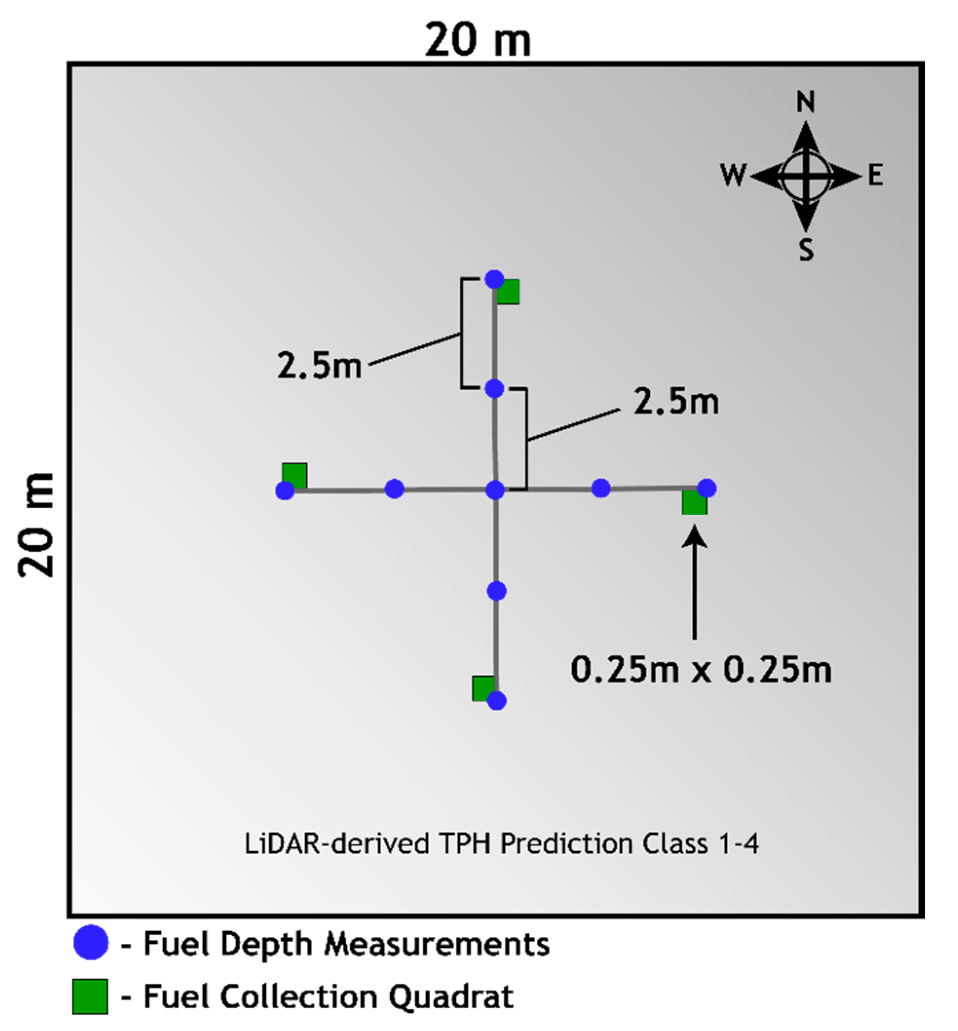
Within each of the 36 sampled plots, fuel size classes were sampled in four quadrats. Once the plot center was located via GPS coordinates, 5-m vectors extending directly north, south, east, and west of the plot center were marked and established as the corner points for the quadrats. For instances in which uncharacteristic site conditions occurred within the quadrats, the frame was reflected over the transect. If this quadrat reflection did not resolve the issue and fuel collection within the quadrat was still not possible, the quadrat was excluded from sampling overall. Situations that would permit quadrat reflection over the transect or exclusion included buried logs, stumps, and rock outcroppings. In addition to the collection of fuels within the 25-cm squared quadrats, the fuel depth of masticated fuels was measured at two locations along the 5-m vectors (2.5 m and 5 m) and at the overall plot center (Figure 4). To measure fuel depths, a cross-section of the forest floor was cleared using a trowel, and the depths were manually recorded. For the depths of the woody/masticated material, any branch or piece of woody debris above the measurement point was included in the depth measurement. Where site conditions prevented the measuring of fuel depths, the depth was measured 0.5 m from the original measurement point moving away from the plot center along the transect. If the depth was still not measurable at the second location, the measurement was omitted. Each of the 36 plots contained four separate fuel collection quadrats and nine fuel depth measurements.
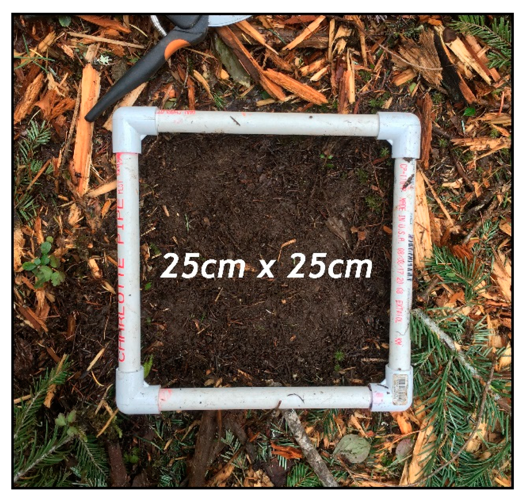
Frames made of PVC pipe measuring 25 cm by 25 cm were built to establish the sampling area extent. Within the 25 × 25-cm collection quadrats, all fuel down to bare mineral soil was gathered, and any pieces extending outside the collection frame were trimmed using hand shears, and thus only pieces completely within the frame were collected (Figure 5). All fuels collected were stored in paper bags labeled by their collection point and were brought back to the lab for detailed fuel composition analysis. Within the sampling quadrats, downed trees and logs were not sampled due to their irregular occurrence and collection difficulty for returning to the lab.
It was assumed that when locating sample plots in the field, there may be instances where mastication, though planned, does not occur. This was a result of inaccessibility, due to the steep or very uneven terrain where the operator chose not to treat the area for safety reasons. In these instances, three supplemental sample points for each classification level of trees per hectare were randomly selected in each of the three stands. If an originally designated sample plot was found to be within an un-masticated area, a randomly selected supplemental sample plot of the same TPH class was selected for sampling instead. These supplemental plots were randomly generated from the remaining available pixels not included in the initial stratification prior to field sampling, using the same method used in the initial plot selection. Supplemental plots were used once in unit 117, four times in unit 120, and four times in unit 147. The final sampled plots across stands 117, 120, and 147 are shown in Figure 6.
2.4. Lab Measurements and Fuel Characterization
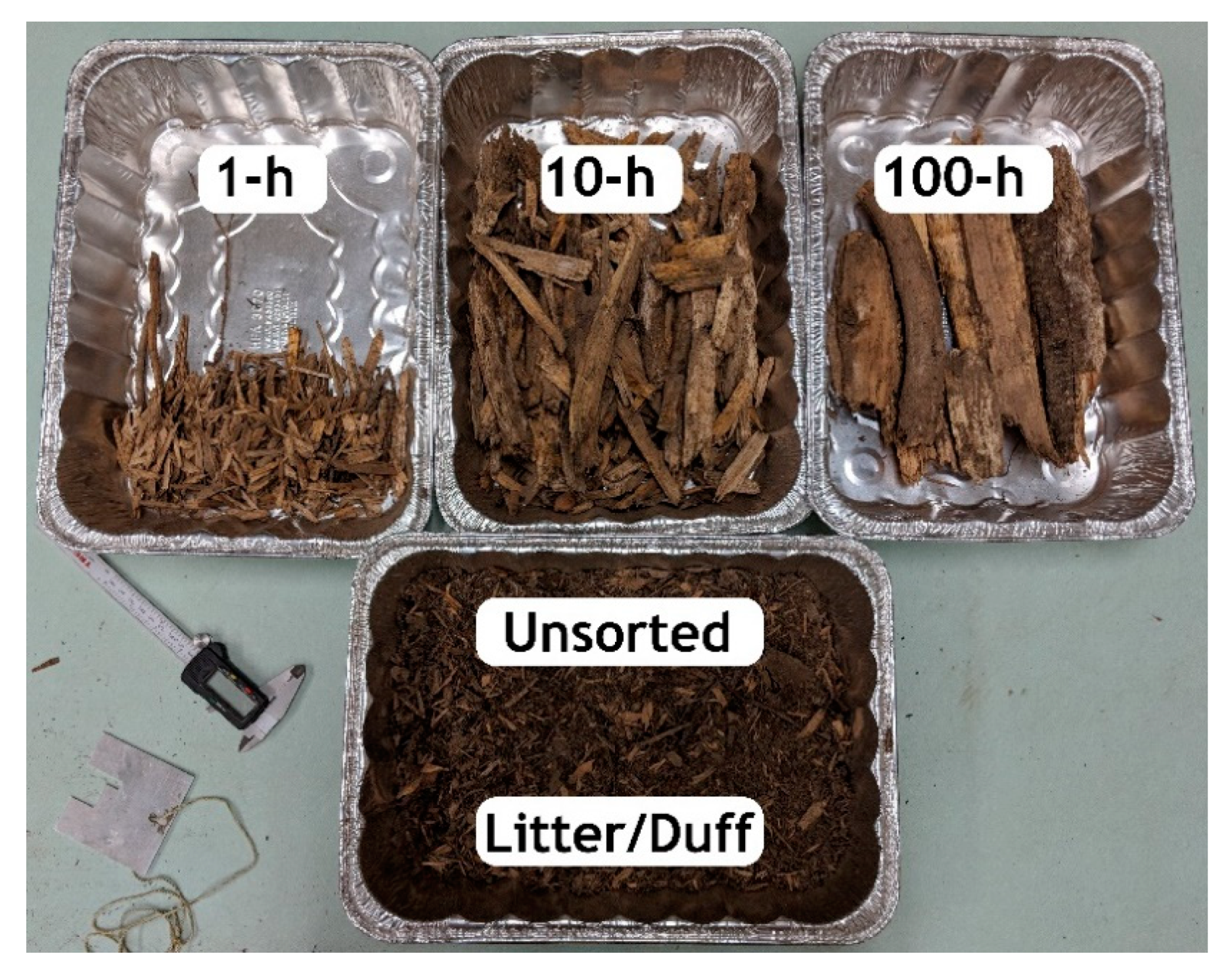
After field sampling was conducted, fuel collection bags were brought back to the lab to be processed by drying and sorting. A total of 133 quadrats of fuel was brought from the field for processing. If all plots had all quadrats collected, there would have been a total of 144. However, some quadrats were excluded from sampling because they were located on rock outcroppings, stumps, or other obstructions. One complete plot of quadrat fuel collections from stand 117, trees per hectare class 1, was misplaced during sampling, which constituted four of the eleven missing quadrat samples. Due to the omitted samples, stand 117 had two plots for trees per hectare class 1, resulting in 35 total plots rather than 36. Each collection sample was oven-dried at 105 degrees Celsius for 48 h, or until the sample weight stabilized, and was then weighted to the nearest gram. All fuels were then sorted, by quadrat, into five time-lag fuel classes: duff/litter and woody/masticated (1-h [<0.64 cm], 10-h [0.64–2.54 cm], 100-h [2.54–7.62 cm] and 1000-h [>7.62 cm]) [56] (Figure 7). Sorted fuels were then individually weighed to the nearest gram to determine the proportion of overall mass that each fuel class represented. These proportions for each quadrat were averaged with corresponding plot quadrats to determine the fuel composition proportions by mass for the entire plot. For each of the 35 sample plots, the fuel bed volume was calculated by multiplying the average of the fuel depths at the nine measured locations within each plot by the dimensions of the collection frame. We then determined the bulk density of the fuels in each plot by dividing the average oven-dried weight of the fuel classes in the four collection quadrats by the corresponding volume. Plot level values were calculated using the averages of each quadrat within the plot for fuel loading (Mg ha−1) for the whole stand and by fuel class, fuel depth (cm), and bulk density (kg m−3).
To assess the correlation between pre-treatment LiDAR-derived forest metrics and post-treatment fuel conditions, all statistical analyses were performed using the R statistical programming environment. Pearson correlation coefficients were calculated to evaluate the strength of association between predictors. Additionally, linear mixed effects models were used to model the relationship between fuel loading following mastication treatments and the trees per hectare, stand density index, and basal area of plots prior to mastication, using the nlme R package [57]. The general equation for mixed effect models is described as:
where β are fixed effects, u are random effects, X is the model matrix for fixed effects, Z is the model matrix for random effects, ε is the vector of errors, R is the variance-covariance matrix of within-individual measurements, and D is the variance-covariance matrix of random effects [58]. In linear mixed effects, models evaluating predictors, stand, and TPH class were treated as random effects, with the TPH class nested within the stand. Random intercepts were used when fitting models. Due to the inconsistency of the mastication treatment in stand 147, two different mixed effects models were fit for each of the LiDAR predictors. One model contained all three stands, while the second model contained only stand 117 and 120. This was in order to avoid potential influential data artifacts associated with the treatment change in stand 147.
3. Results
Parameter estimates for the random forest models used in the pretreatment derivation of forest characteristics from LiDAR metrics for 20 × 20-m pixels are shown in Table 1. In this study, an acceptable maximum root-mean-square error (RMSE) of 50% of the prediction means was used based on values derived in previous studies [59,60]. The RMSE was within the acceptable range for the density (TPH), basal area (m2 ha−1), and stand density index models. For the random forest model predicting stand volume (m3 ha−1), an RMSE of 166.93 was about 54% of the predicted mean and just outside of the desired range. Predicted volume was therefore excluded from use in subsequent analyses. Model accuracies for forest metrics were 71.5%, 77.4%, 74.3%, and 79% for trees per hectare, basal area, volume, and stand density index, respectively, which are comparable to those obtained by Falkowski et al. [61] and Hudak et al. [60]. These pretreatment maps of predicted stand characteristics provided the basis for study plot selection and the subsequent regression modeling of post-treatment fuel loading.
Table 2 shows the summary data of the stands for the fuel collection as averages of the sampled plots and quadrats within each stand. Surface fuel loadings range from 9.3–83.4 Mg ha−1, 1.8–34.5 Mg ha−1, 5.4–80.5 Mg ha−1, 0–48.1 Mg ha−1, and 0–8.2 Mg ha−1 for litter/duff, to 1-h, 10-h, 100-h and 1000-h fuel classes, respectively, across all plots and stands. Fuel depths ranged from 6.4–26.3 cm and bulk densities ranged from 22.2 to 154.2 kg m−3. Across all plots, there was a significant (p = 0.029) moderate positive (0.369) correlation between trees per hectare and fuel loading (Mg m−1), found by performing a Pearson’s correlation test. Additionally, there was a positive (0.3577) and significant (p = 0.0349) correlation between SDI and fuel loading. No significant relationship was found between pre-treatment TPH and bulk density of resulting fuels (kg m−3); SDI and bulk density of resulting fuels; basal area (m2 h−1) and loading or bulk density; nor between pre-treatment total volume (m3 ha−1) and fuel loading or bulk density (Table 3). Based on the results of the correlation tests, the linear mixed effects model was fitted to evaluate the relationship of pre-treatment TPH and the resulting fuel loads as well as SDI and the resulting fuel loads.
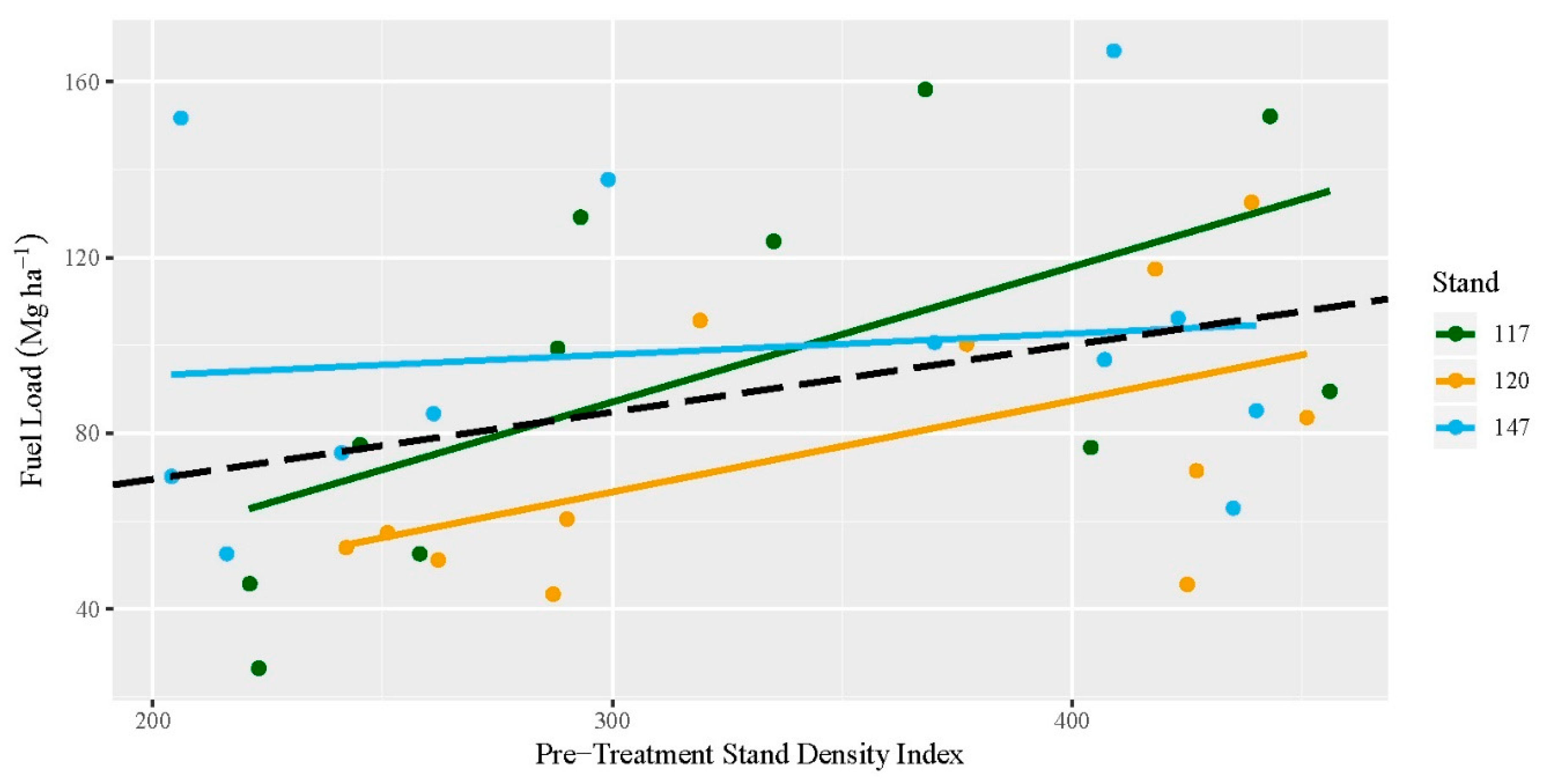
The linear mixed effects models predicting the total fuel loading of all time-lag classes from pre-treatment TPH showed no significant relationship between the two factors (test statistic = 0.05318, df = 22, p-value = 0.0527) when accounting for all three stands. In the reduced model, pre-treatment trees per hectare and fuel loading were significant (p-value = 0.0066) (Table 4). The linear mixed effects models predicting the total fuel loading of all time-lag classes from pre-treatment SDI showed significant relationships between the two factors for all three units (p = 0.0477) and when assessing stand 117 and 120 alone (p = 0.0337) (Table 4). Figure 8 shows the associated relationships between SDI and the resulting fuel load for all three units. The black line represents the regression line of the complete data set and the individual regression line for each stand.
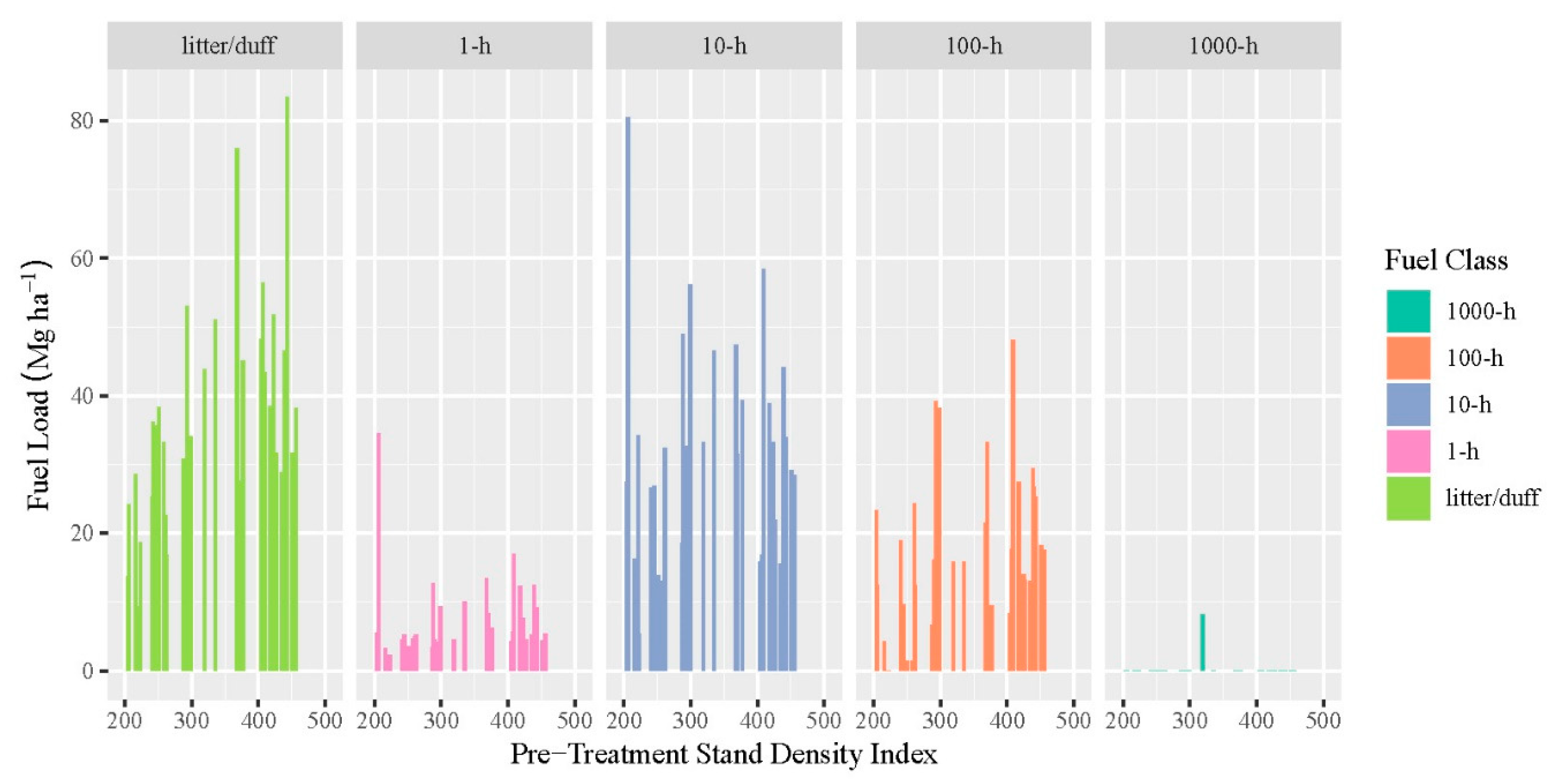
Additional linear mixed effects models were developed to further assess the impact of pre-treatment TPH and SDI on resulting fuels loads for each of the 5 time-lag fuel classes (litter/duff, 1-h, 10-h, 100-h, 1000-h). Only the litter/duff fuel class loading was found to be significantly correlated to pre-treatment trees per hectare for all three stands (Table 5). The litter/duff fuel class is generally independent of the mastication process, as most fuels in this class were present before treatment. However, when assessing stands 117 and 120, litter/duff (p = 0.0242), 1-h (p = 0.0232), and 100-h (p = 0.0059) were found to be significant. When assessing the relationship between SDI and the resulting fuel loading across all five time-lag cases, the model containing all three units showed that both litter/duff (p = 0.0042) and 100-h (p = 0.0293) were significant, while the model describing units 117 and 120 showed that only 100-h (p = 0.0476) was significant. The data for the SDI model are shown in Figure 9.
Our second research objective explored whether the in-plot distribution of masticated fuels among the five time-lag fuel classes was impacted by the stand density of the plot prior to treatment. Mixed effects models were developed to assess these questions, with results being found in Table 6. 10-h fuels in the sampled plots were the only fuel class found to change significantly as the pre-treatment TPH changed (test statistic = −0.01581, p = 0.0178, df = 22). SDI was shown to have a significant relationship with post-mastication fuel loading for both the 10-h (p = 0.0302) and 100-h (p = 0.0406) fuel classes (Table 6).
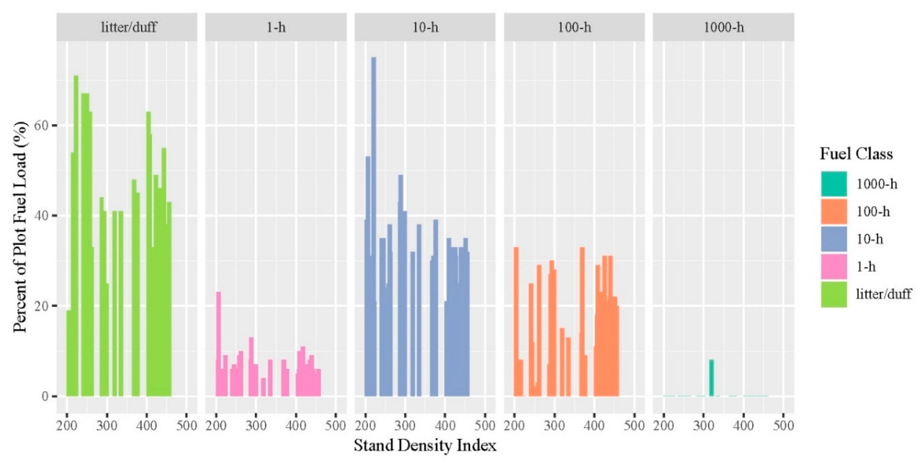
The data distribution for the five time-lag classes as a percentage across the range of stand density indices and fuel loading are shown in Figure 10. Woody and mulched fuels (1-h, 10-h, 100-h, and 1000-h) were found to be between 30–85% of the overall fuel loads across all plots, which shows the variability found within the stands. 1-h, 10-h, 100-h, and 1000-h fuels contained 6–27%, 36–94%, 0–57%, and 0–13% of the woody and mulched fuels, respectively. On average, woody fuels made up about 58.2% of the overall surface fuel loading across all sites, with 1-h, 10-h, 100-h, and 1000-h fuel classes averaging 7.5%, 33.2%, 17.3%, and 0.2% of the loading, respectively.
4. Discussion
Total surface fuel loadings varied widely across our study plots (26.4 to 158.2 Mg ha−1), with woody/masticated surface fuels representing a similarly wide range (7.7 to 127.5 Mg ha−1). Across all stands and plots, total surface fuel loading averaged 89.8 Mg ha−1, and woody surface fuels averaged 53.9 Mg ha−1. These total surface fuel loads were similar to those reported by Stephens and Moghaddas [16] in the Sierra Nevada Mountains (87.1 and 93.8 Mg ha−1), Reiner et al. [18] in the Sierra Nevada (81.6 Mg ha−1), Kane et al. [14] at study sites in Northern California and southwestern Oregon (83.6, 83.8 and 71.1 Mg ha−1), and Hood and Wu [17] in the Northern Rockies (82.0–95.9 Mg ha−1), but were higher than those reported by Brewer et al. [62] in mixed conifer Idaho stands (58.4 Mg ha−1) and lower than those reported by Battaglia et al. [10] in mixed conifer stands in Colorado (110.4 Mg ha−1). This finding was not surprising, as masticated fuel beds and characteristics have a wide variability across sites and regions. The attempt to develop the surface fuel prediction model at a 20 × 20-m resolution in this study was meant to help address this site variability.
Based on results reported by previous mastication studies, the average total fuel depth of 16.7 cm recorded in the mixed conifer stands we studied was significantly higher than those in Battaglia et al. [10], but only slightly higher than those shown by Stephens and Moghaddas [16]: 14.6 and 14.7 cm. All fuel sampling in this study occurred within a month of mastication treatment, so fuels were still green at the time of collection and had not settled to the forest floor, whereas sampling of masticated fuels for other studies occurred 2–6 years post-mastication [10,14]. These temporal changes in masticated fuel beds make the generalization of loadings difficult, especially across broad geographic extents. For example, a recently masticated stand may indicate greater fuel depths than a stand masticated several years ago, due to the decomposition and deterioration of fuel structural integrity. The additional compaction of fuel beds over time as they settle may affect subsequent fire behavior. Therefore, the development of the model estimating surface fuel characteristics directly after masticating would provide a consistent expectation of fuel loads, as was done in this study.
4.1. Relationship between Pre-Treatment Stand Characteristics and Fuel Loading
Through the analysis performed across the three stands we studied—117, 120, and 147—no significant relationship was found between overall fuel loading following mastication and the pre-treatment tree per hectare we derived from LiDAR. However, SDI was found to be a significant predictor variable for post-mastication fuel loading when accounting for all management units and time-lag classes jointly. Initially, we expected to see an increase in the fuel loading as the pre-treatment TPH increased. It was believed that, given a consistent prescription implementation, greater TPH would result in more fuel, as a greater number of standing trees were mulched to meet treatment objectives. The contrary findings for absolute stand density may have resulted from the inconsistency in the initial treatment of stand 147, which was then corrected. When excluding stand 147, increasing pre-treatment TPH resulted in greater loading, as expected. However, even when including data from stand 147, the p-value of 0.0526 was just outside the level of significance needed to reject the null. The significance of both mixed effects models for SDI (p = 0.0477 and p = 0.0337) indicates fuel loading may be more accurately predicted using a metric that accounts for both tree size and number, as opposed to simply using trees per hectare where only the number of stems is accounted for.
Stand 147 was the first stand treated and was initially treated to prescription specifications. It was found that once treatment began, the original degree to which large downed woody debris was to be treated was operationally infeasible due to the increased treatment time. Further, stand 147 contained a small pocket of lodgepole pine killed by beetle, with a significant portion of downed trees which were, under the original treatment specs, to be masticated heavily. This resulted in a larger amount of masticated fuels in plots with relatively low stand densities.
The decision to retain stand 147 in the analysis was made to maximize the data available for assessment and provide a realistic portrayal of the large variability of mastication treatments. As a relatively new treatment option being deployed over large areas, it is likely that similar inconsistency in operational treatments may occur during implementation and administration of mechanical fuel treatments, particularly as operators familiarize themselves with prescription requirements in new treatment areas. However, when the treatment prescription and execution was consistent for the entire stand, as seen in stands 117 and 120, a clear relationship between pre-treatment trees per hectare and fuel loading was seen. Given the potential for variability of mastication treatments and the heterogeneity of stand conditions in practice, the predictive success of SDI in a “real-world” management scenario is valuable for future modeling efforts.
Given the extent of our results, it remains unclear if a relationship exists between the fuel loading following mastication treatments and the pre-treatment stand density based solely on TPH or stand basal area, but SDI is a useful predictor. In mastication, the conservation of mass must be considered, as materials are not removed from the stand after treatment but rearranged in different physical forms. A larger masticated tree will understandably produce a larger amount of masticated material than a tree of smaller size. For example, two stands may both have similar numbers of trees per unit area, but one stand may have a larger average tree diameter than the other. If both stands are treated to the same prescription and reduced to a defined tree per unit area, it would be expected that the stand with the larger average stand diameter would produce heavier masticated fuel loadings. Accounting for both stem number per unit area and tree size in a single pre-treatment stand metric, SDI addresses this issue. Therefore, alternative approaches to modeling landscape scale fuel loading following mastication based on pre-treatment stand conditions that incorporate both stem numbers and size may offer improved prediction in future research and should be the focus of future study design and implementation.
When assessing the fuel loading for each time-lag class (litter/duff, 1-h, 10-h, 100-h, 1000-h), the litter duff class showed a significant relationship for the TPH and SDI models (Table 5). This may be a result of greater stand density, leading to higher amounts of organic material and litter on the forest floor. In all, minimal 1000-h fuels were collected at the plots, limiting the available data for the particular classes and making predictions difficult. This finding corroborates Kane et al.’s [11], who found that the plot-based method of surface fuel sampling does not assess a large enough area to effectively capture the presence of 1000-h fuels as well as planar intersect methods. This is a result of 1000-h fuels generally occurring less frequently than other fuel classes in fuel beds.
4.2. Relationship between Pre-Treatment Stand Density and Fuel Class Distribution
As shown above (Table 6), only the 10-h fuels expressed as a percentage of the overall surface fuel loading were found to change as the TPH increased. It is unclear why the percentage of 10-h fuels would decrease with increasing TPH, but this may be a result of changes in treatment implementation. For example, the operator may spend less time masticating trees to maintain production in a denser stand, resulting in an increase in the proportion of larger fuel classes. It would be expected that, with one fuel class decreasing over increasing TPH, another fuel class would increase. This was seen in the SDI model, where the significant decrease in 10-h fuels (coefficient = −0.04616, p = 0.0302) was matched by a significant increase in 100-h fuels (coefficient = 0.042089, p = 0.0406). With increasing stand density, it is possible the operator attempted to maintain the desired operational production by decreasing the time spent masticating each tree. As a result, trees would be masticated less thoroughly, and there would be a larger percentage of larger fuel particles. The 10-h fuel class accounted for the highest fuel loads across all classes by a considerable amount in our study, which is consistent with other studies [10,14]. Given the variability of the mastication as a whole, and the wide range of fuel loadings across 1-h, 10-h, 100-h, and 1000-h fuel classes, our results show that the distribution of surface fuels among time-lag fuel classes was not clearly modeled as a function of changes in TPH and SDI alone, apart from the 10-h and 100-h classes, in the case of this study.
4.3. Study Limitations and Future Work
Mastication is a highly variable operation impacted by many factors, and it is understood that there are some limitations to the scope of our research that should be addressed in future studies. One factor to consider in future applications of this methodology is the pixel size at which the LiDAR metrics were predicted. In the study development, it was believed that maximizing prediction resolution was the best option. Mastication, however, is a variable process, resulting in a scattered distribution of fuels on the forest floor. The directionality, travel distance, and particle size of comminuted materials may be affected by the type of mastication head (disk vs. drum), equipment type (all surface vehicle vs. excavator carrier), equipment horsepower, boom or attachment height, local topography within the stand, or other factors. While the sampling method developed by Hood and Wu [17] attempts to address the variability in stand and site conditions by sampling across multiple quadrats within the same plot, what was not accounted for in our study design was the possibility of fuels from adjoining pixels being distributed inter-pixel. During the observation of the treatment, fuels were clearly distributed more irregularly and further than anticipated. The 20 m × 20-m pixels used in the plot selection may have been too small to limit the influence of surrounding pixels in the resulting fuels found during sampling. For instance, a stand with a high stand density may have resulted in fuels initially in the stand as standing trees being distributed to an adjacent stand of a lower stand density, or to areas within the same stand that were not accounted for in our sampling design. During sampling, it would then appear that the pixel with the lower stand density was responsible for creating greater fuel loads than was possible. By decreasing the resolution and increasing the pixel size, this may be avoided.
In the fuel collection process, future studies should incorporate a hybrid, plot-based, and planar intersect method, as suggested by Kane et al. [14]. Doing so may help to ensure a more accurate representation of the fuel classes, as 1-h and 10-h fuels are more accurately represented in plot-based sampling [14], while planar intersect methods cover greater proportions of the overall masticated area, properly representing the 100-h and 1000-h fuels that may be missed in plot-based approaches [11]. Supplemental planar intersect sampling was not performed in this study due to the small 20 m × 20-m pixel size and the concern that sufficiently long intersect paths would extend too far to sample plot edges and be impacted by the distribution of fuels from adjacent pixels. Increasing the pixel size used in predicting the stand characteristics from the LiDAR, as described above, would enable an easier implementation of supplemental planar intersect sampling. Additionally, due to the variability of fuel distribution across the forest floor, plot-based sampling in future studies should use larger sampling quadrats than the 25 × 25-cm ones used in this study. Alternatively, a larger number of 25 × 25-cm sampling quadrats may also provide a greater representation of overall fuel variability within the sampling plot. The goal in using a smaller sampling quadrat in this study than those described in previous studies [17,63] was to create an efficient and effective sampling procedure. However, larger quadrats will provide a greater representation of overall surface fuel loadings and should be studied.
5. Conclusions
The ability to quickly, efficiently, and effectively predict surface fuel loads resulting from mastication treatments is a valuable tool, as increased implementation of this management technique occurs. A variety of research and management questions regarding the longevity, fuel bed characteristics, and fire behavior within masticated fuels exist and will increase in relevance as LiDAR data become more widespread, along with the use of mastication to reduce fuels in stands where commercial thinning may be infeasible or more difficult to implement administratively. Existing methods for predicting surface fuel loads rely on intensive, time-consuming sampling following treatment. While existing methods are effective for estimating fuel loading, methods based on remote sensing may help managers to proactively plan and predict post-treatment fire behavior over large areas to optimize treatments in ways that incorporate topography and stand adjacency.
The results from this study showed that pre-treatment stand density metrics that account only for tree number per unit area, such as TPH, were not good predictors of resulting surface fuel loads following mechanical fuel treatments with the sampling design and sample size we evaluated. TPH prior to treatment was not directly related to the distribution of fuel time-lag classes within the fuel bed, although the percentage of 10-h fuels could be predicted from pre-treatment conditions. However, stand density index, which accounts for both the relative stem number and DBH of the stand, effectively predicts post-treatment fuel loading across the whole study area. Further, SDI predicted that as the density of a stand increases, a greater percentage of the overall fuel load consisted of 100-h fuels, while 10-h fuels decreased in percentage, likely a result of operational adjustments. Future modeling efforts to predict post-mastication fuel loading should account for both the stem number and stem size, as stand density alone may not provide the necessary predictive ability. Attempting to predict resulting fuels from the number of trees per unit area alone does not account for variable volumes of materials in trees of different diameters. Stand density measures, such as SDI, provide greater insight into stand composition and overall stand biomass, which is significant when predicting fuel load volumes resulting from the physical conversion of standing biomass to surface-based mulched materials. Two stands with identical TPH may contain varying amounts of biomass as standing trees, whereas it is expected that two stands with identical SDI would have the same amount of overall biomass given similar forest types and species.
We believe that revisiting these methods, while taking into account the sampling considerations mentioned in the discussion, is an important undertaking and could lead to the increased implementation and effectiveness of mastication treatments. The rapid onset of LiDAR-derived models to map individual-tree locations and stem characteristics, coupled with onboard GNSS mapping of spatially, explicit, real-time equipment activities, offer the promise of improved high-resolution fuel bed prediction in the immediate future. Further expanding the scope of the field sampling to multiple, unique forest types, operators, and prescriptions would better capture the variability associated with the masticated surface fuel loads. Future work should address these factors more closely, though the determination of their impacts will likely require sampling at a higher intensity than that performed in this study, or with a sampling design that directly accounts for the spatial resolution at which comminuted material is scattered as a function of localized stand density, treatment prescription, topography, equipment type and size, and the pattern of equipment movements.
Author Contributions
Conceptualization, R.M.B. and R.F.K.; methodology, R.M.B. and R.F.K.; formal analysis, R.M.B. and R.F.K.; writing—original draft preparation, R.M.B.; writing—review and editing, R.M.B., R.F.K.; visualization, R.M.B.; supervision, R.F.K.; funding acquisition, R.F.K. All authors have read and agreed to the published version of the manuscript.
Funding
This research was funded by Joint Fire Sciences, JFSP PROJECT ID: 13-1-05-7.
Acknowledgments
The authors would like to thank Tom McLeod and Bob Vermey from the Nez Perce-Clearwater National Forest for help in facilitating and locating field sampling locales. Further, we would like to thank Mackenzie Smith for the time given during the field sampling. Publication of this article was funded by the University of Idaho’s Open Access Publishing Fund. All authors have read and agreed to the published version of the manuscript.
Conflicts of Interest
The authors declare no conflict of interest.
References
- Reinhardt, E.D.; Keane, R.E.; Calkin, D.E.; Cohen, J.D. Objectives and considerations for wildland fuel treatment in forested ecosystems of the interior western United States. For. Ecol. Manag. 2008, 256, 1997–2006. [Google Scholar] [CrossRef]
- Hartsough, B.R.; Abrams, S.; Barbour, R.J.; Drews, E.S.; McIver, J.D.; Moghaddas, J.J.; Schwilk, D.W.; Stephens, S.L. The economics of alternative fuel reduction treatments in western United States dry forests: Financial and policy implications from the National Fire and Fire Surrogate Study. For. Policy Econ. 2008, 10, 344–354. [Google Scholar] [CrossRef]
- Oliveira, T.M.; Barros, A.M.G.; Ager, A.A.; Fernandes, P.M. Assessing the effect of a fuel break network to reduce brunt area and wildfire risk transmission. Int. J. Wildland Fire 2016, 25, 619–632. [Google Scholar] [CrossRef]
- Alcasena, F.J.; Ager, A.A.; Salis, M.; Day, M.A.; Vega-Garcia, C. Optimizing prescribed fire allocation for managing fire risk in central Catalonia. Sci. Total. Environ. 2018, 621, 872–885. [Google Scholar] [CrossRef] [PubMed] [Green Version]
- Agee, J.K.; Skinner, C.N. Basic principles of forest fuel reduction treatments. For. Ecol. Manag. 2005, 211, 83–96. [Google Scholar] [CrossRef]
- Stephens, S.L.; Moghaddas, J.J.; Edminster, C.; Fiedler, C.E.; Haase, S.; Harrington, M.; Keeley, J.E.; Knapp, E.E.; McIver, J.D.; Metlen, K.; et al. Fire treatment effects on vegetation structure, fuels, and potential fire severity in western U.S. forests. Ecol. Appl. 2009, 19, 305–320. [Google Scholar] [CrossRef] [Green Version]
- Agee, J.K. The influence of forest structure on fire behavior. In Proceedings of the 17th Annual Forest Vegetation Management Conference, Redding, CA, USA, 16–18 January 1996; pp. 52–68. [Google Scholar]
- Stephens, S.L. Effects of fuels and silvicultural treatments on potential fire behavior in mixed conifer forests of the Sierra Nevada, CA. For. Ecol. Manag. 1998, 105, 21–34. [Google Scholar] [CrossRef]
- Huggett, R.J., Jr.; Abt, K.L.; Shepperd, W. Efficacy of mechanical fuel treatments for reducing wildfire hazard. For. Policy Econ. 2008, 10, 408–414. [Google Scholar] [CrossRef]
- Battaglia, M.A.; Rocca, M.E.; Rhoades, C.C.; Ryan, M.G. Surface fuel loadings within mulching treatments in Colorado conifer forests. For. Ecol. Manag. 2010, 260, 1557–1566. [Google Scholar] [CrossRef]
- Kane, J.M.; Knapp, E.E.; Varner, J.M. Variability in loadings of mechanically masticated fuel beds in northern California and southwestern Oregon. In Fuels Management-How to Measure Success: Conference Proceedings, Proceedings RMRS-P-41, Portland, OR, USA, 28–30 March 2006; Andrews, P.L., Butler, B.W., Eds.; U.S. Department of Agriculture, Forest Service, Rocky Mountain Research Station: Fort Collins, CO, USA, 2006; pp. 341–350. [Google Scholar]
- Jain, T.; Graham, R.T.; Sandquist, J.; Butler, M.; Brockus, K.; Frigard, D.; Cobb, D.; Sup-Han, H.; Halbrook, J.; Denner, R.; et al. Restoration of northern Rocky Mountain moist forests: Integrating fuel treatments from the site to the landscape. In Integrated Restoration of Forested Ecosystems to Achieve Multiresource Benefits, Proceedings of the 2007 National Silviculture Workshop, Gen. Tech. Rep. PNW-GTR-733, Ketchikan, AK, USA, 7–10 May 2007; Deal, R.L., Ed.; U.S. Department of Agriculture, Forest Service, Pacific Northwest Research Station: Portland, OR, USA, 2008. [Google Scholar]
- Jain, T.; Sikkink, P.; Keefe, R.; Byrne, J. To Masticate or Not: Useful Tips for Treating Forest, Woodland, and Shrubland Vegetation; Gen. Tech. Rep. RMRS-GTR-381; U.S. Department of Agriculture, Forest Service, Rocky Mountain Research Station: Fort Collins, CO, USA, 2018.
- Kane, J.M.; Varner, J.M.; Knapp, E.E. Novel fuelbed characteristics associated with mechanical mastication treatments in northern California and south-western Oregon, USA. Int. J. Wildland Fire 2009, 18, 688–697. [Google Scholar] [CrossRef] [Green Version]
- Kreye, J.K.; Brewer, N.W.; Morgan, P.; Varner, J.M.; Smith, A.M.S.; Hoffman, C.M.; Ottmar, R.D. Fire behavior in masticated fuels: A review. For. Ecol. Manag. 2014, 314, 193–207. [Google Scholar] [CrossRef]
- Stephens, S.L.; Moghaddas, J.J. Fuel treatment effects on snags and course woody debris in a Sierra Nevada mixed conifer forest. For. Ecol. Manag. 2005, 214, 53–64. [Google Scholar] [CrossRef]
- Hood, S.; Wu, R. Estimating fuelbed loadings in masticated areas. In Fuels Management-How to Measure Success: Conference Proceedings, Proceedings RMRS-P-41, Portland, OR, USA, 28–30 March 2006; Andrews, P.L., Butler, B.W., Eds.; U.S. Department of Agriculture, Forest Service, Rocky Mountain Research Station: Fort Collins, CO, USA, 2006; pp. 333–340. [Google Scholar]
- Reiner, A.L.; Vaillant, N.M.; Fites-Kaufman, J.; Dailey, S.N. Mastication and prescribed fire impacts on fuels in a 25-year old ponderosa pine plantation, southern Sierra Nevada. For. Ecol. Manag. 2009, 258, 2365–2372. [Google Scholar] [CrossRef]
- Arroyo, L.A.; Pascual, C.; Manzanera, J.A. Fire models and methods to map fuel types: The role of remote sensing. For. Ecol. Manag. 2008, 256, 1239–1252. [Google Scholar] [CrossRef] [Green Version]
- Keane, R.E.; Burgan, R.; van Wagtendonk, J. Mapping wildland fuels for fire management across multiple scales: Integrating remote sensing, GIS, and biophysical modelling. Int. J. Wildland Fire 2001, 10, 301–319. [Google Scholar] [CrossRef]
- Rollins, M.G.; Keane, R.E.; Parsons, R.A. Mapping fuel and fire regimes using remote sensing, ecosystem simulation, and gradient modeling. Ecol. Appl. 2004, 14, 75–95. [Google Scholar] [CrossRef] [Green Version]
- Falkowski, M.J.; Gessler, P.E.; Morgan, P.; Hudak, A.T.; Smith, A.M.S. Characterizing and mapping forest fire fuels using ASTER imagery and gradient modeling. For. Ecol. Manag. 2005, 217, 129–146. [Google Scholar] [CrossRef] [Green Version]
- Maltamo, M.; Eerikainen, K.; Pitkanen, J.; Hyyppa, J.; Vehmas, M. Estimation of timber volume and stem density based on scanning laser altimetry and expected tree size distribution functions. Remote Sens. Environ. 2004, 90, 319–330. [Google Scholar] [CrossRef]
- Andersen, H.; McGaughey, R.J.; Reutebuch, S.E. Estimating forest canopy fuel parameters using LIDAR data. Remote Sens. Environ. 2005, 94, 441–449. [Google Scholar] [CrossRef]
- Skowronski, N.S.; Clark, K.L.; Duveneck, M.; Hom, J. Three-dimensional canopy fuel loading predicted using upward and downward sensing LiDAR systems. Remote Sens. Environ. 2011, 115, 703–714. [Google Scholar] [CrossRef]
- Erdody, T.L.; Moskal, L.M. Fusion of LiDAR and imagery for estimating forest canopy fuels. Remote Sens. Environ. 2010, 114, 725–737. [Google Scholar] [CrossRef]
- Chen, Y.; Zhu, X.; Yebra, M.; Harris, S.; Tapper, N. Development of a predictive model for estimating forest surface fuel load in Australian eucalypt forests with LiDAR data. Environ. Model. Softw. 2017, 97, 61–71. [Google Scholar] [CrossRef]
- Jakubowski, M.K.; Guo, Q.; Collins, B.; Stephens, S.; Kelly, M. Predicting surface fuel models and fuel metrics using lidar and CIR imagery in a dense, mountainous forest. Photogramm. Eng. Remote Sens. 2013, 79, 37–49. [Google Scholar] [CrossRef] [Green Version]
- Mutlu, M.; Popescu, S.C.; Stripling, C.; Spencer, T. Mapping surface fuel models using lidar and multispectral data fusion for fire behavior. Remote Sens. Environ. 2008, 112, 274–285. [Google Scholar] [CrossRef]
- Van Aardt, J.A.N.; Arthur, M.; Sovkoplas, G.; Swetnam, T.L. LiDAR-based estimation of forest floor fuel loads using a novel distributional approach. In Proceedings of the SilviLaser 2011, Hobart, Australia, 16–20 October 2011. [Google Scholar]
- Mutlu, M.; Popescu, S.C.; Zhao, K. Sensitivity analysis of fire behavior modeling with LIDAR-derived surface fuel maps. For. Ecol. Manag. 2008, 256, 289–294. [Google Scholar] [CrossRef]
- Kramer, H.A.; Collins, B.M.; Kelly, M.; Stephens, S.L. Quantifying ladder fuels: A new approach to using LiDAR. Forests 2014, 5, 1432–1453. [Google Scholar] [CrossRef]
- Skowronski, N.; Clark, K.; Nelson, R.; Hom, J.; Patterson, M. Remotely sensed measurements of forest structure and fuel loads in the Pinelands of New Jersey. Remote Sens. Environ. 2007, 108, 123–129. [Google Scholar] [CrossRef]
- Garcia, M.; Riano, D.; Chuvieco, E.; Salas, J.; Danson, F.M. Multispectral and lidar data fusion for fuel type mapping using Support Vector Machine and decision rules. Remote Sens. Environ. 2011, 115, 1369–1379. [Google Scholar] [CrossRef]
- Koetz, B.; Morsdorf, F.; van der Linden, S.; Curt, T.; Allgower, B. Multi-source land cover classification for forest fire management based on imaging spectrometry and lidar data. For. Ecol. Manag. 2008, 256, 263–271. [Google Scholar] [CrossRef]
- Price, O.F.; Gordon, C.E. The potential for LiDAR technology to map fire fuel hazard over large areas of Australian forests. J. Environ. Manag. 2016, 181, 663–673. [Google Scholar] [CrossRef]
- Garcia, M.; Saatchi, S.; Casas, A.; Koltunov, A.; Ustin, S.L.; Ramirez, C.; Balzter, H. Extrapolating forest canopy fuel properties in the California Rim Fire by combining airborne LiDAR and Landsat OLI data. Remote Sens. 2017, 9, 394. [Google Scholar] [CrossRef] [Green Version]
- Chen, Y.; Zhu, X.; Yebra, M.; Harris, S.; Tapper, N. Strata-based forest fuel classification for wild fire hazard assessment using terrestrial LiDAR. J. Appl. Remote Sens. 2016, 10, 046025. [Google Scholar] [CrossRef] [Green Version]
- Vermey, B.; (Nez Perce-Clearwater National Forest Red River Ranger District, Elk City, ID, USA). Personal communication, 2017.
- Dixon, G.E. Essential FVS: A User’s Guide to the Forest Vegetation Simulator. Internal Report; U.S. Department of Agriculture, Forest Service, Forest Management Service Center: Fort Collins, CO, USA, 2002.
- Breiman, L. Random Forests. Mach. Learn. 2001, 45, 5–32. [Google Scholar] [CrossRef] [Green Version]
- Liaw, A.; Wiener, M. Classification and Regression by randomForest. R News 2002, 2, 18–22. [Google Scholar]
- Becker, R.M.; Keefe, R.F.; Anderson, N.M.; Eitel, J.U.H. Use of LiDAR-derived landscape parameters to characterize alternative harvest system options in the Inland Northwest. Int. J. For. Eng. 2018, 29, 179–191. [Google Scholar] [CrossRef]
- R Core Team. R: A Language and Environment for Statistical Computing. R Foundation for Statistical Computing; R Core Team: Vienna, Austria, 2020; Available online: https://www.R-project.org/ (accessed on 12 February 2020).
- Breiman, L. Manual on Setting Up, Using, and Understanding Random Forests v3.1; Statistics Department University of California: Berkeley, CA, USA, 2002; Available online: https://www.stat.berkeley.edu/~breiman/RandomForests/cc_manual.htm (accessed on 13 February 2020).
- Brosofske, K.D.; Froese, R.E.; Falkowski, M.J.; Banskota, A. A review of methods for mapping and prediction of inventory attributes for operational forest management. For. Sci. 2014, 60, 733–756. [Google Scholar] [CrossRef]
- Cinaroglu, S. Comparison of performance of decision tree algorithms and random forest: An application of OECD countries health expenditures. Int. J. Comput. Appl. 2016, 138, 37–41. [Google Scholar] [CrossRef]
- Belgiu, M.; Dragut, L. Random forest in remote sensing: A review of applications and future directions. ISPRS J. Photogramm. 2016, 114, 24–31. [Google Scholar] [CrossRef]
- Evans, J.S.; Murphy, M.A. rfUtilities: Random Forests Model Selection and Performance Evaluation. R Package Version 2.0-1. Available online: http://rdocumentation.org/packages/rfUtilities/versions/2.0-1.html. (accessed on 15 May 2017).
- McGaughey, R.J. FUSION/LDV: Software for LiDAR Data Analysis and Visualization. February 2013–FUSION Version 3.60; USDA Forest Service, Pacific Northwest Research Station, University of Washington: Seattle, WA, USA, 2017; Available online: http://forsys.sefs.uw.edu/fusion/fusionlatest.html (accessed on 15 June 2017).
- Reineke, L.H. Perfecting stand-density index for even-aged forests. J. Agric. Res. 1933, 46, 627–638. [Google Scholar]
- Woodall, C.W.; Miles, P.D.; Vissage, J.S. Determining maximum stand density index in mixed species stands for strategic-scale stocking assessments. For. Ecol. Manag. 2005, 216, 367–377. [Google Scholar] [CrossRef]
- Shaw, J.D. Reineke’s stand density index: Where are we and where do we go from here? In Proceedings of the Society of American Foresters National Convention, Fort Worth, TX, USA, 19–23 October 2005; Society of American Foresters: Bethesda, MD, USA, 2006. [Google Scholar]
- Ducey, M.J.; Knapp, R.A. A stand density index for complex mixed species forests in the northeastern United States. For. Ecol. Manag. 2010, 260, 1613–1622. [Google Scholar] [CrossRef]
- VanderSchaaf, C.L. Reineke’s stand density index: A quantitative and nonunitless measure of stand density. In Proceedings of the 15th Biennial Southern Silvicultural Research Conference, Hot Springs, AK, USA, 17–20 November 2008; Southern Research Station: Asheville, NC, USA, 2013; pp. 577–579. [Google Scholar]
- Brown, J.K. Handbook for Inventorying Downed Woody Material; Intermountain Forest and Range Experiment Station: Ogden, UT, USA, 1974.
- Pinheiro, J. Fit and Compare Gaussian Linear and Nonlinear Mixed-Effects Models. 2020. Available online: https://svn.r-project.org/R-packages/trunk/nlme/ (accessed on 15 August 2019).
- Laird, N.M.; Ware, J.H. Random-effects models for longitudinal data. Biometrics 1982, 38, 963–974. [Google Scholar] [CrossRef] [PubMed]
- Fekety, P.A.; Falkowski, M.J.; Hudak, A.T.; Jain, T.B.; Evans, J.S. Transferability of lidar-derived basal area and stem density models within a Northern Idaho ecoregion. Can. J. Remote Sens. 2018, 44, 131–143. [Google Scholar] [CrossRef]
- Hudak, A.T.; Bright, B.C.; Pokswinski, S.M.; Loudermilk, E.L.; O’Brien, J.J.; Hornsby, B.S.; Klauberg, C.; Silva, C.A. Mapping forest structure and composition from low-density LiDAR for informed forest, fuel, and fire management at Englin Air Force Base, Florida, USA. Can. J. Remote Sens. 2016, 42, 411–427. [Google Scholar] [CrossRef]
- Falkowski, M.J.; Hudak, A.T.; Crookston, N.L.; Gessler, P.E.; Uebler, E.H.; Smith, A.M.S. Landscape-scale parameterization of a tree-level forest growth model: A k-nearest neighbor imputation approach using LiDAR data. Can. J. For. Res. 2010, 40, 184–199. [Google Scholar] [CrossRef]
- Brewer, N.W.; Smith, A.M.S.; Hatten, J.A.; Higuera, P.H.; Hudak, A.T.; Ottmar, R.D.; Tinkman, W.T. Fuel moisture influences on fire-altered carbon in masticated fuels: An experimental study. J. Geophys. Res. Biogeosci. 2013, 118, 30–40. [Google Scholar] [CrossRef] [Green Version]
- Lyon, Z.D.; Morgan, P.; Stevens-Rumann, C.S.; Sparks, A.M.; Keefe, R.F.; Smith, A.M.S. Fire behavior in masticated forest fuels: Lab and prescribed fire experiments. Int. J. Wildland Fire 2018, 27, 280–292. [Google Scholar] [CrossRef]
Figure 1.
Mini-excavator with a horizontal shaft masticator head used in mastication treatments.

Figure 2.
Visual comparison of treated stands and a representation of surface fuels in stand 147 before (left pane) and after (right pane) adjustments to treatment intensity.
Figure 2.
Visual comparison of treated stands and a representation of surface fuels in stand 147 before (left pane) and after (right pane) adjustments to treatment intensity.

Figure 3.
Crooked River LiDAR acquisition area and Orogrande T.S. mastication stands located in the Nez Perce-Clearwater National Forest, ID, USA.
Figure 3.
Crooked River LiDAR acquisition area and Orogrande T.S. mastication stands located in the Nez Perce-Clearwater National Forest, ID, USA.

Figure 4.
Destructive plot-based sampling design used for surface fuel collection and field measurements.
Figure 4.
Destructive plot-based sampling design used for surface fuel collection and field measurements.

Figure 5.
Fuel collection quadrat used in destructive fuel sampling.

Figure 6.
Field sampling plots within masticated stands 117, 120, and 147, selected based on stand density (TPH) prior to treatment.
Figure 6.
Field sampling plots within masticated stands 117, 120, and 147, selected based on stand density (TPH) prior to treatment.

Figure 7.
Sorting of dried surface fuels based on time-lag class (1-h, 10-h, 100-h, 1000-h, litter/duff).
Figure 7.
Sorting of dried surface fuels based on time-lag class (1-h, 10-h, 100-h, 1000-h, litter/duff).

Figure 8.
Surface fuel loading (Mg ha−1) of all sampled plots by pre-treatment stand density index (SDI). The black dotted line represents the regression for all data, and the colored solid lines indicate the regression lines for each stand individually.
Figure 8.
Surface fuel loading (Mg ha−1) of all sampled plots by pre-treatment stand density index (SDI). The black dotted line represents the regression for all data, and the colored solid lines indicate the regression lines for each stand individually.

Figure 9.
Surface fuel loading (Mg ha−1) distribution for all sample plots by pre-treatment stand density index (SDI) arranged by time-lag fuel class.
Figure 9.
Surface fuel loading (Mg ha−1) distribution for all sample plots by pre-treatment stand density index (SDI) arranged by time-lag fuel class.

Figure 10.
Percentage of total surface fuel load for all sample plots by pre-treatment stand density index (SDI) arranged by time-lag fuel class.
Figure 10.
Percentage of total surface fuel load for all sample plots by pre-treatment stand density index (SDI) arranged by time-lag fuel class.


Table 1.
Random forest model quality assessment for pre-treatment forest metrics.
| Random Forest | Prediction Mean | RMSE | R-Squared | Accuracy (%) |
|---|---|---|---|---|
| Stand Density (TPH) | 468.00 | 217.36 | 0.55 | 71.5 |
| Basal Area (m2 ha−1) | 30.56 | 12.95 | 0.63 | 77.4 |
| Total Volume (m3 ha−1) | 307.99 | 165.35 | 0.57 | 76.3 |
| Stand Density Index (SDI) | 299.17 | 110.296 | 0.45 | 79.0 |
Table 2.
Stand-level summary data representing stand averages and standard errors for pre-treatment trees per hectare and post-treatment destructive plot-based surface fuel characteristics for stands 117, 120, and 147.
Table 2.
Stand-level summary data representing stand averages and standard errors for pre-treatment trees per hectare and post-treatment destructive plot-based surface fuel characteristics for stands 117, 120, and 147.
| Stand | Pre-TPH Avg. (SE) | Fuel Loading (Mg ha−1) Avg. (SE) | Fuel Depth (cm) Avg. (SE) | Bulk Density (kg m−3) Avg. (SE) | |||||
|---|---|---|---|---|---|---|---|---|---|
| Litter/ Duff | 1-h | 10-h | 100-h | 1000-h | Total | ||||
| 117 | 530 | 43.4 | 6.7 | 30.3 | 13.2 | 0.0 | 93.7 | 15.6 | 59.0 |
| (77) | (6.7) | (1.2) | (4.3) | (3.7) | (0.0) | (13.1) | (1.5) | (5.8) | |
| 120 | 515 | 31.9 | 5.5 | 25.3 | 13.4 | 0.7 | 76.8 | 16.1 | 48.2 |
| (77) | (3.3) | (1.0) | (3.2) | (2.6) | (0.7) | (8.8) | (1.2) | (4.4) | |
| 147 | 516 | 32.9 | 9.1 | 34.3 | 22.8 | 0.0 | 99.2 | 18.4 | 59.2 |
| (93) | (3.6) | (2.5) | (5.9) | (3.6) | (0.0) | (10.4) | (1.5) | (10.6) | |
Table 3.
Pearson’s correlation assessments for pre-treatment forest characteristics and surface fuel characteristics following mastication treatments, where T is the t-test statistic and DF is the degrees of freedom.
Table 3.
Pearson’s correlation assessments for pre-treatment forest characteristics and surface fuel characteristics following mastication treatments, where T is the t-test statistic and DF is the degrees of freedom.
| Correlation | T | DF | p-Value | Coefficient |
|---|---|---|---|---|
| Density (TPH)/Loading (Mg ha−1) | 2.2812 | 33 | 0.0291 | 0.3691 |
| Density (TPH)/Bulk Density (kg m−3) | 1.566 | 33 | 0.1269 | 0.2630 |
| Volume (m3 ha−1)/Loading (Mg ha−1) | 1.8018 | 33 | 0.0807 | 0.2993 |
| Volume (m3 ha−1)/Bulk Density (kg m−3) | 1.1251 | 33 | 0.2687 | 0.1922 |
| Basal Area (m2 h−1)/Loading (Mg ha−1) | 1.9676 | 33 | 0.0576 | 0.3240 |
| Basal Area (m2 h−1)/Bulk Density (kg m−3) | 1.3492 | 33 | 0.1865 | 0.2286 |
| Stand Density Index/Loading (Mg ha−1) | 2.2004 | 33 | 0.0349 | 0.3577 |
| Stand Density Index/Bulk Density (kg m−3) | 1.8702 | 33 | 0.0704 | 0.3096 |
Table 4.
Mixed effects model summary assessing pre-treatment trees per hectare (TPH) and stand density index (SDI) impact on fuel loading (Mg ha−1) post-mastication. The influence of stand 147 on the overall significance of the factors is shown.
Table 4.
Mixed effects model summary assessing pre-treatment trees per hectare (TPH) and stand density index (SDI) impact on fuel loading (Mg ha−1) post-mastication. The influence of stand 147 on the overall significance of the factors is shown.
| Stand 117, 120, 147 | ||||
|---|---|---|---|---|
| Predictor | Estimate | Std. Error | DF | p-Value |
| TPH | 0.05318 | 0.025974 | 22 | 0.0527 |
| SDI | 0.16736 | 0.079809 | 22 | 0.0477 |
| Stand 117, 120 | ||||
| Predictor | Estimate | Std. Error | DF | p-Value |
| TPH | 0.09524 | 0.029924 | 14 | 0.0066 |
| SDI | 0.227069 | 0.09647 | 14 | 0.0337 |
Table 5.
Mixed effects model summary assessing pre-treatment trees per hectare (TPH) and stand density index (SDI) impact on fuel loading (Mg ha−1) sorted by time-lag fuel class post-mastication. The influence of stand 147 on the overall significance of the predictors for each of the time-lag classes is shown.
| Stand 117, 120, 147 | |||||
|---|---|---|---|---|---|
| Fuel Class | Predictor | Estimate | Std. Error | DF | p-Value |
| Litter/Duff | TPH | 0.0033284 | 0.0010120 | 22 | 0.0034 |
| 1-h | TPH | 0.0000789 | 0.0003873 | 22 | 0.8405 |
| 10-h | TPH | 0.0000719 | 0.0009999 | 22 | 0.9433 |
| 100-h | TPH | 0.0015591 | 0.0008138 | 22 | 0.0685 |
| 1000-h | TPH | −0.0000106 | 0.0000901 | 22 | 0.9072 |
| Litter/Duff | SDI | 0.096484 | 0.030246 | 22 | 0.0042 |
| 1-h | SDI | 0.001137 | 0.012228 | 22 | 0.9267 |
| 10-h | SDI | 0.004637 | 0.031801 | 22 | 0.8854 |
| 100-h | SDI | 0.0562922 | 0.024141 | 22 | 0.0293 |
| 1000-h | SDI | −0.0007695 | 0.002888 | 22 | 0.7924 |
| Stand 117, 120 | |||||
| Fuel Class | Predictor | Estimate | Std. Error | DF | p-Value |
| Litter/Duff | TPH | 0.0038925 | 0.0015411 | 14 | 0.0242 |
| 1-h | TPH | 0.0008194 | 0.0003215 | 14 | 0.0232 |
| 10-h | TPH | 0.0021593 | 0.0010591 | 14 | 0.0608 |
| 100-h | TPH | 0.0025606 | 0.0007890 | 14 | 0.0059 |
| 1000-h | TPH | −0.0000245 | 0.0001527 | 14 | 0.8747 |
| Litter/Duff | SDI | 0.095805 | 0.046646 | 14 | 0.0592 |
| 1-h | SDI | 0.019364 | 0.010368 | 14 | 0.0829 |
| 10-h | SDI | 0.058114 | 0.034173 | 14 | 0.1111 |
| 100-h | SDI | 0.057603 | 0.026532 | 14 | 0.0476 |
| 1000-h | SDI | −0.002020 | 0.004787 | 14 | 0.6794 |
Table 6.
Mixed effects model summary assessing pre-treatment stand density (TPH) and stand density index (SDI) impact on the percentage of total fuel load (Mg ha−1) by time-lag fuel class.
Table 6.
Mixed effects model summary assessing pre-treatment stand density (TPH) and stand density index (SDI) impact on the percentage of total fuel load (Mg ha−1) by time-lag fuel class.
| Stand Density (TPH) | ||||
|---|---|---|---|---|
| Fuel Class | Estimate | Std. Error | DF | p-Value |
| Litter/Duff | 0.00560 | 0.009796 | 22 | 0.5736 |
| 1-h | −0.00190 | 0.0021351 | 22 | 0.3825 |
| 10-h | −0.01581 | 0.006169 | 22 | 0.0178 |
| 100-h | 0.01161 | 0.006380 | 22 | 0.0823 |
| 1000-h | −0.0001 | 0.000850 | 22 | 0.9072 |
| Stand Density Index (SDI) | ||||
| Fuel Class | Estimate | Std. Error | DF | p-Value |
| Litter/Duff | 0.00766 | 0.03098 | 22 | 0.8069 |
| 1-h | −0.007688 | 0.006679 | 22 | 0.2620 |
| 10-h | −0.04619 | 0.019931 | 22 | 0.0302 |
| 100-h | 0.042089 | 0.019346 | 22 | 0.0406 |
| 1000-h | −0.0007254 | 0.0027224 | 22 | 0.7924 |
© 2020 by the authors. Licensee MDPI, Basel, Switzerland. This article is an open access article distributed under the terms and conditions of the Creative Commons Attribution (CC BY) license (http://creativecommons.org/licenses/by/4.0/).
Share and Cite
MDPI and ACS Style
Becker, R.M.; Keefe, R.F. Prediction of Fuel Loading Following Mastication Treatments in Forest Stands in North Idaho, USA. Sustainability 2020, 12, 7025. https://0-doi-org.brum.beds.ac.uk/10.3390/su12177025
AMA Style
Becker RM, Keefe RF. Prediction of Fuel Loading Following Mastication Treatments in Forest Stands in North Idaho, USA. Sustainability. 2020; 12(17):7025. https://0-doi-org.brum.beds.ac.uk/10.3390/su12177025
Chicago/Turabian StyleBecker, Ryer M., and Robert F. Keefe. 2020. "Prediction of Fuel Loading Following Mastication Treatments in Forest Stands in North Idaho, USA" Sustainability 12, no. 17: 7025. https://0-doi-org.brum.beds.ac.uk/10.3390/su12177025
Note that from the first issue of 2016, this journal uses article numbers instead of page numbers. See further details here.