Seasonality Effect Analysis and Recognition of Charging Behaviors of Electric Vehicles: A Data Science Approach

Abstract

Electric vehicles (EVs) presence in the power grid can bring about pivotal concerns regarding their energy requirements. EVs charging behaviors can be affected by several aspects including socio-economics, psychological, seasonal among others. This work proposes a case study to analyze seasonal effects on charging patterns, using a public real-world based dataset that contains information from the aggregated load of the total charging stations of Boulder, Colorado. Our approach targets to forecast and recognize EVs demand considering seasonal factors. Principal component analysis (PCA) was used to provide a visual representation of the variables and their contribution and the correlation among them. Then, twelve classification models were trained and tested to discriminate among seasons the charging load of electric vehicles. Later, a benchmark stage is presented for regression as well as for classification results. For regression models, examined through Mean Absolute Percentage Error (MAPE) and Root Mean Square Error (RMSE), the random Forest provides better prediction than quasi-Poisson model widely. However, it was observed that for large variations in electric vehicles’ charging load, quasi-Poisson fits better than random forest. For the classification models, evaluated through Accuracy and the Area under the Curve, the Lasso and elastic-net regularized generalized linear (GLMNET) model provided the best global performance with accuracy up to 100% when evaluated on the test dataset. The results of this work offer great insights for enhancing demand response strategies that involve PEV charging regarding charging habits across seasons.

1. Introduction

As non-conventional renewable power sources increases its contribution to the energy supply mix, transportation becomes the main responsible for CO₂ emissions. Road transport sector accounts for about 25% of greenhouse gases (GHG) emissions. Nowadays, several long and short term policies have been taken to mitigate GHG emissions from increasing fuel efficiency to the use of alternative fuels to power vehicles. For instance, the Paris Agreement, proposed by the United Nations (UN) and enforced in November 2016, has as main objective to limit the global average temperature below two-celsius degrees above pre-industrial levels. The transport sector is called to play an essential role in the process of decarbonizing the energy system. The most recent trends lean toward sustainable road transportation throughout the electrification of its propulsion systems [1]. It is the most promising solution to fulfil the climate change goals traced by the UNs. Recent rigorous regulations and customers’ demand for high fuel economy pointed to accelerated developments of different alternative powertrain solutions, especially electric vehicles (EVs) [2]. EVs are more efficient than traditional cars with internal combustion engines (ICEs) and even natural gas-powered vehicles because they have less moving parts and they can be charged from any energy source of electricity [3]. Thus, massive use of them may help reduce GHG emission. Consequently, there have been several policies implemented worldwide to increase the adoption of EVs [4]. As a result, in 2016, 750 thousand new vehicles were sold, and today there are more than 2 million vehicles on the roads [5].

Although the numerous barriers EVs have to face, their massive adoption worldwide currently is possible thanks to some catalysts including sustained growth in renewable energies, battery price falls, and battery technology improvements [6]. Electricity coming from renewable sources including solar-photovoltaic (PV), wind among others which are experiencing the lowest prices in the last decades [7]. As well, battery technologies cost experienced its lowest cost in history, 85% cheaper than in 2010 and is forecasted that by 2023, their average prices will fall up to 90% compared with 2010 prices [8]. These reductions are thanks to increasing order size and market uptake in battery electric vehicles sales. Therefore, EVs users should take advantage of this reduction to charge their vehicles from green sources and truly achieve an environmentally friendly solution to decarbonize the transportation sector. Nevertheless, there is a significant share still of EVs users that uses the conventional power grid to charge their vehicles. Thus their impact on distribution grids depict an essential challenge to face [9,10,11,12].

Over the last decades, several approaches have been developed until today to solve problems related to load balancing and capacity planning due to large-scale EVs penetration [13]. For instance, demand-side response (DR) provides optimal charging schemes to arrange the demand of EVs strategically to the lowest electricity prices [14]. However, even though the high performance and accuracy of these strategies, many factors still have not been taken into account when modelling users’ load charging habits. For instance, EV charging loads are sensitive to seasons, and seasonal factors have not been widely taken into account in recent studies. Therefore, it is necessary to analyze these factors that can affect owners’ charging habits. Zhao et al. proposed a strategy for domestic electric vehicle charging loads by explaining the key factors that can affect users charging behavior, taking into account the seasonal factors [15]. Boston and Werthman analyzed charging and driving behavior of Ford plug-in electric vehicles with real-world data. Their findings shows that electricity prices, local charging infrastructure, and seasonal weather changes may affect driving behavior and then charging habits [16]. Ul-Haq et al. performed a stochastic approach to model EVs charging patterns associated with residential load considering several cases among which, season factors where included [17]. Their results state that charging habits changes across seasons.

With the rapid growth of EVs, several concerns arise regarding their power requirements. A potential solution to prevent unexpected load demand, is load forecasting [18,19,20,21,22]. Early stages on EVs load forecasting are based on the charging behavior of EVs owners [23]. Markov Chains and Monte Carlo (MC) simulations are methods that describe well the holiday and seasonal periods [24]. For instance, Wang et al. used MC algorithms to forecast the electric vehicle charging load based on charging frequency [25]. In Gerossier’s et al. study, they modelled charging habits, and thus they obtained probabilistic forecasts of the aggregated load. Besides, they evaluate the impact of EVs on the grid by 2030 by assuming that future charging behavior follows current habits [26]. However, load prediction is somehow uncertainty due to the nature of overdispersed data. Some other studies focused on spatial and time distribution of EVs charging stations (CS) demand [27,28,29]. Currently, advances in machine and deep learning techniques aid largely to model the fluctuation of CS’s demand.

Rapid uptake of EVs worldwide has led to a large amount of charging data, and machine learning methods represents a potential solution to deal with it. There are several methods used to forecast EVs charging load such as support vector machines (SVM) [30], and recurrent methods including long-short-term memory (LSTM) neural networks [31] and extreme gradient boost (XGBOOST) [32]. However, data is scarce to handle the randomness of EVs load, and it depicts a significant obstacle for the majority of time series prediction algorithms. That randomness is explained from several stochastic factors, including weather conditions and occupant behaviors [33,34]. Since these factors affect a considerable proportion of electricity load forecasting, their contribution has been studied through correlation analysis based on non-parametric residual data from autoregressive (AR) models [35] and behavior surveys [36]. Recent studies have proved the last mentioned. For instance, Amara et al. developed an approach to model residual load for household short-term load forecasting (STFL) through an Adaptative Circular Conditional Expectation (ACCCE) combined with linear models (LM) [35]. Wang et al. conducted a study to model customer behavior for effective load forecasting by using Sparse Continuous Conditional Random Fields (SCCRF) to apply hierarchical cluster analysis [37] further.

Differently from the above-listed methods, random forest (RF) models have been largely applied to power load prediction on the user-side [38]. RF can provide higher and more stable results than SVM in load prediction [39]. RF is an additive method based on several decision trees which has been widely proved to be a powerful approach to forecast electrical load [40]. Therefore, in this work, we used RF to demand forecasting on the user-side and to deal with possible overdispersion on data, we used a Quasi-Poisson (QPM) models.

This work considered seasonal factors to perform short-term load forecasting (STLF) and to discriminate the demand of EVs among seasons. The research question to be occupied by this work is: Do the seasons shape the way users charge their vehicles?. Our approach differs from the related ones published in the literature mainly on the use of both regression and classification approaches, since most of them rely on the use of one or the other, but not on using both. However, most studies in this regard only considers information on the vehicle or charging station side. Then we decided to join the average temperature to the variables to be analyzed. This study trained and tested not only multiple classifiers (12) capable of discriminating charging behaviors among seasons, but also different (3) regression models to forecast the energy consumption considering various scenarios. Also, an effect analysis of charging behaviors across seasons was developed using principal components, to provide a visual representation of the data in a two-dimensional space and also to analyze the relationship and contribution of variables. Afterwards, a feature importance technique was used to evaluate the importance of each variable. Finally, statistical analysis is provided by using analysis of variance (ANOVA) and Chi-square test to test with a 95% of certainly the hypothesis of the null-hypothesis: EVs load and the charging time varies depending on seasons factors.

The results of this work can aid in the planning of power distribution systems at large scale and also in providing valuable information to supply strategies such as demand response strategies in practical applications.

The structure of this paper is as follows: Section 2 presents the methodology used for exploratory analysis, feature importance, classification and regression procedures as well as the metrics used for their evaluation. Then, Section 5 presents the results. Finally, Section 6 concludes the paper.

2. Methods

We propose an approach for load forecasting and classification from an analysis on a real-world dataset. The whole process from preprocessing to results presentation was done in RStudio (Version 1.1.442). Several machine learning tools to reach the last mentioned were used. An exploratory analysis was developed to find a possible correlation among the variables and to provide a general picture of the data behavior. Two regression models, including QPM and RF and several classification models (12) were tuned with the 10-fold cross-validation algorithm to find the optimal parameters to minimize performance metrics. Regression and classification procedures were conducted separately.

2.1. Regression Models

2.1.1. Quassi-Poisson Regression

The current study proposes a Quasi-Poisson regression model to forecast EVs charging demand. Among several methods of regression, a quasi-Poisson model (QPM) shows to be functional to account for overdispersed data, which is reasonable during EVs connection to the grid because charging behavior depends on several social, economical among other factors. QPMs can be understood as generalized linear models (GLMs). Suppose that Y is a random variable such that:

$$E\left(Y\right)=\mu$$

$$var\left(Y\right)=\theta \mu$$

where $E\left(Y\right)$ is the expectation or the mean of Y distribution and $var\left(Y\right)$ the variance of Y. $\theta$ is an overdispersion parameter. QPMs models can be easily evaluated since they are characterized by the first two statistical moments: mean and variance.

2.1.2. Random Forest Regression

The random forest model is an additive-based model that makes predictions by merging decisions from a sequence of base models. Mathematically, additive models can be described as:

$$g\left(x\right)=f0\left(x\right)+f1\left(x\right)+f2\left(x\right)+...$$

where the final model $g\left(x\right)$ is the result of simple decision trees $f\left(x\right)$. This technique is family of ensemble models and it provides better predictive performance since it eliminates correlation between decision trees by randomly selecting samples and features. The use of RF based models aids on the task of reducing over-fitting and increasing the accuracy.

2.2. Classification Models

We used several classification models including the conventional ones: support vector machines (SVM), linear discriminant analysis (LDA and SLDA), multinomial regression (MN), decision trees (DT), and naive Bayes (NB) and recurrent-based models including: extreme gradient boost (XGBTREE), boosted logistic regression (BLR). However, ensemble models such as Lasso and elastic-net regularized generalized linear models (GLMNET) and bagging trees (TBAG) were used also. These classifiers were trained and tested over the test data with a 10-folds cross-validation algorithm.

3. Data Preparation

Data preprocessing represents a fundamental stage of data analysis since it transforms the data into cleaned forms for high-profit purposes. Once the data was acquired, the process of cleaning it started. First, categorical variables were added only to analyze charging behaviors from further statistical analysis depending on temporal characteristics including weekdays, weekends and seasonality. Also, continuous information related to diary average temperature data were added to find a possible correlation between charging behavior of EVs users and ambient temperature. The rest of the variables were not modified. A summary of the final variables are shown in

Table 1. Data description.

Data Name	Description	Symbol
Date	Date EV charging station ports were used.
Number of sessions	Number of times the charging ports were used on the listed date.	NOS
Unique drivers	Number of unique individual drivers using the charging station on the particular listed date.	UD
Number of ports	The total number of city-owned EV charging ports for the particular listed date.	NOP
Energy [kWh]	The amount of energy that has been dispensed by the charging stations on the particular listed date.	KWH
Accumulated energy [MWh]	The sum of all energy that has been dispensed by the charging stations since the beginning of 2018 up to the listed date.	ACE
GHG savings [Kg]	Estimated emissions avoided based on the energy dispensed and gasoline saved by the charging stations on the listed date.	GHGS
Accumulated GHG [Kg]	The sum of all GHG savings frpm the beginning of 2018 up to the listed date.	ACGHC
Charging time [Min]	The number of minutes any vehicle was plugged in and actively charging on the particular listed date.	CTM
Gasoline savings [Gal]	,Estimated gallons of gasoline saved based on charging time on the paticular listed date.	GSGS
Mean temperature *	Diary ambient temperature	TEMP
Day	Indicates the current day i.e., monday, thursday, and so on.	DAY
Weekday *	1/0 indicates whether it is a weekday	WDAY
Weekend *	1/0 indicates whether it is a weekend	WEEK
Seasonality *	From Winter to Autumn	SEAS

Information marked with * correspond to additional data joined by the author.

.

4. Case Analysis

This section presents information regarding aggregated data of the city-operated public charging stations (44) in Boulder, Colorado from 1 January 2018 to 28 February 2019 presented in [41]. Also, results of an exploratory and feature importance analysis developed on the dataset as well as an analysis per season are presented in this section. Finally, the classification and forecasting models, as well as their performance metrics, are listed.

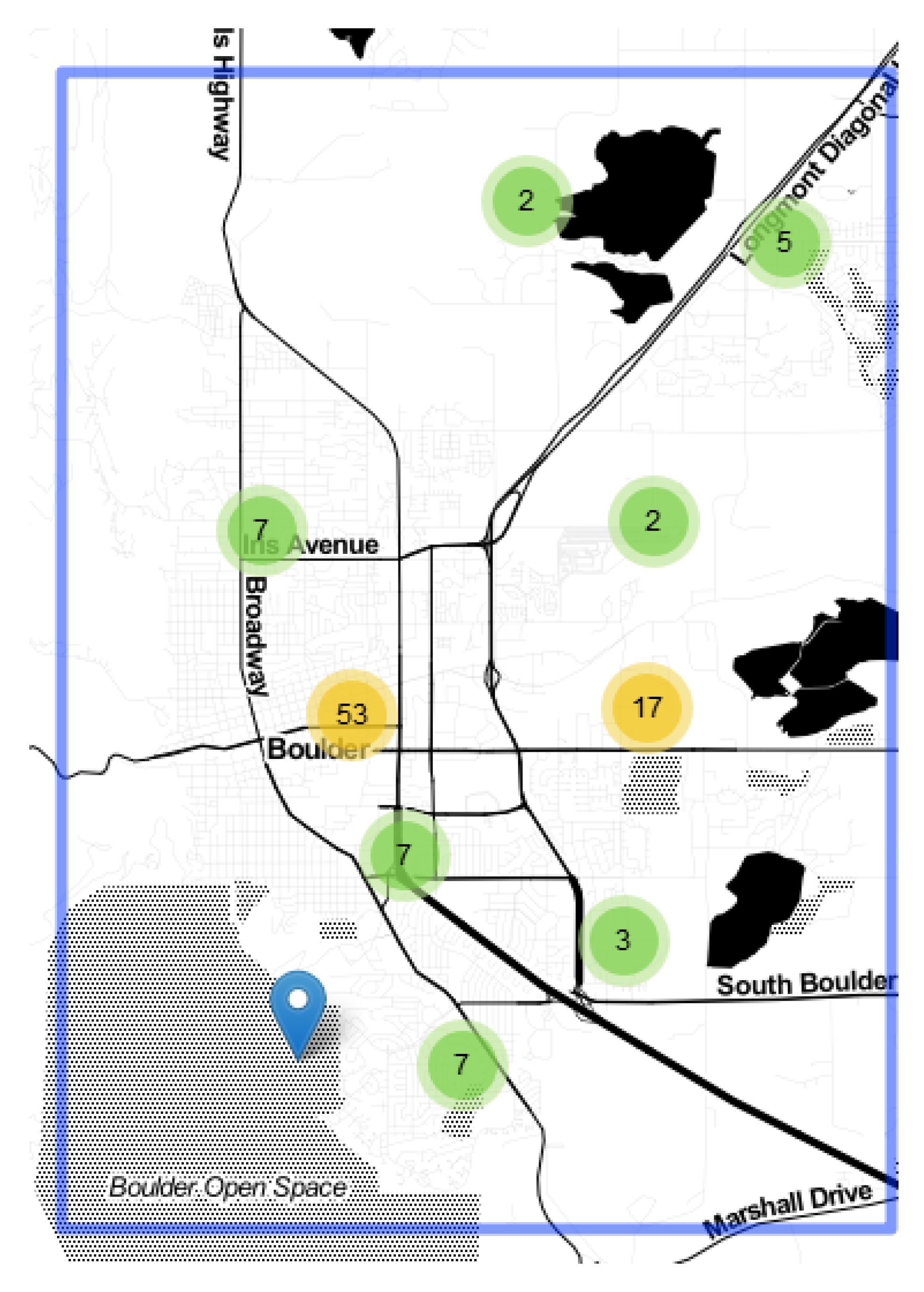
4.1. EVs Charging Stations in Boulder

The Colorado market for EVs has rapidly grown from 20 vehicles in 2011 to more than 3100 in early 2014. According to the ZEV sales dashboard, at middles 2017 10.930 EVs were surpassing in more than three times the amount of them in 2014 [42]. This state is well-prepared to fulfil the challenge of electrifying its road transport. For instance, the local government proposes several well-defined strategies, including charging infrastructure based on mature renewable, vehicle grant programs, among others. With these and several more strategies, this state has emerged as one of the top ten EV markets in the USA [43,44]. This trend is expected to continue growing to a projected amount of 940,000 EVs in Colorado by 2030. Particularly, Boulder precedes California in the number of registered EVs per 1000 residents (2.6 vs 1.4). This city has promoted EVs usage and thus charging stations since 2010 with the enforcement of local projects such as The Boulder SmartGrid Plug-In Electric/Hybrid Vehicles [45].

Figure 1 illustrates the distribution of the charging stations existing in Boulder. The numbers inside the color markers indicate the number of charging stations in the zone. It must be noted that during the time horizon considered in this approach, the amount of stations were 44 in the city, however, to date, the number of stations increased by twice and a bit more.

From the above listed information, EVs load demand is rapidly growing and Figure 2 illustrates its behavior on the last year. This tendency is expected to continue, and therefore it represents an important challenge as not the total CS of boulder are powered by renewable sources.

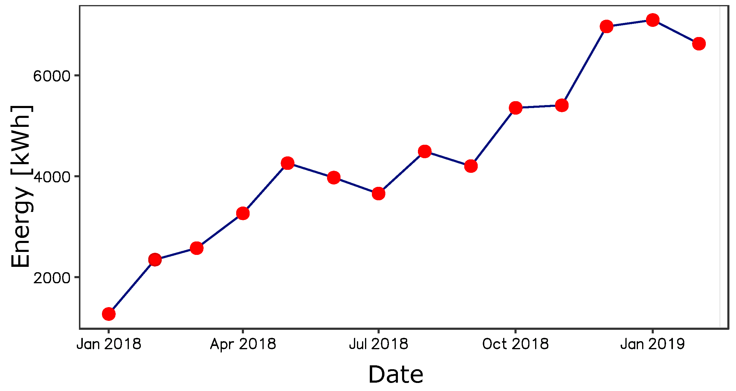
4.2. Exploratory Analysis

We used principal component analysis (PCA) to provide a visual representation of the data. Before PCA, the data were classified by the amount of charging sessions. Only the two first principal components (PCs) were selected as they represent the 72.2% of the information. Figure 3 shows a visual representation of diary observations in a new orthogonal space composed of the two PCs above mentioned. On the one hand, points on the plot are the observations, and their colour is related to the number of charging sessions. On the other hand, information related to the level of contribution of each variable is highlighted with colours being red the maximum. The larger the value of the contribution, the more the variable contributes to the selected principal components.

Thus, the variable which provides less information is CTM followed by ACGHC. As was expected, most of low-frequency charging sessions (Red points) are located in the majority on the third quadrant. This location minimizes the bulk of the variables since they are in the opposite direction of growth of them. This behavior keeps for the rest of the charging sessions groups, more charging sessions, more energy consumption, number of ports used. The opposite growing directions of CTM and TEMP may suggest that they have an inverse relationship.

Figure 4 illustrates a heatmap of daily KWH versus CTM and NOP. It allows observing the energy demand of CS depending on weekdays and weekends. Thus, critical days are visible in terms of energy demand. For instance, most of the ports are used on Monday, Wednesday, and Thursday. Additionally, most of the EVs users lasted for 320 min or more to charge their vehicles from Thursday to Friday.

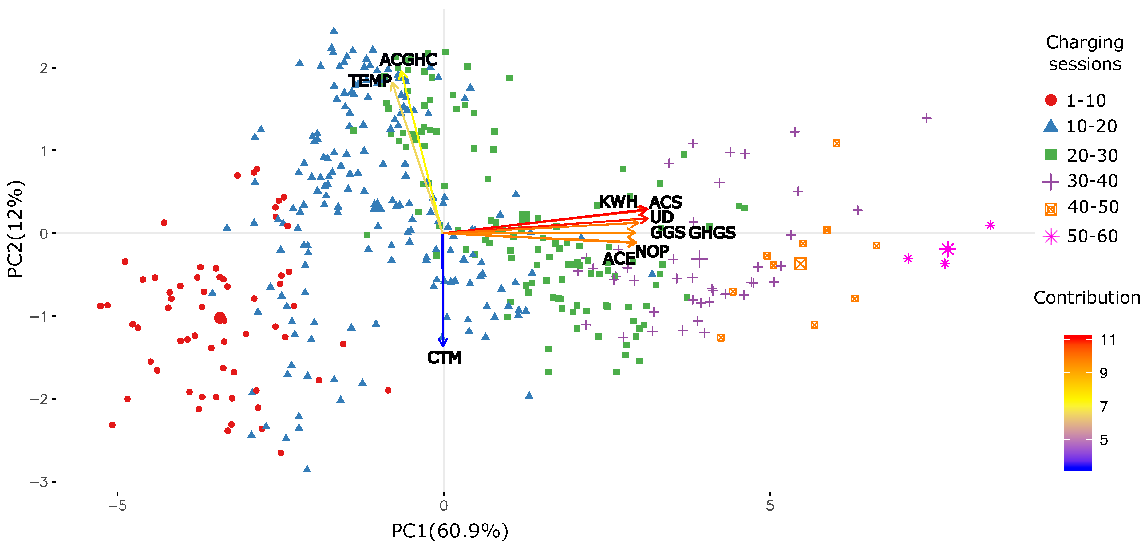
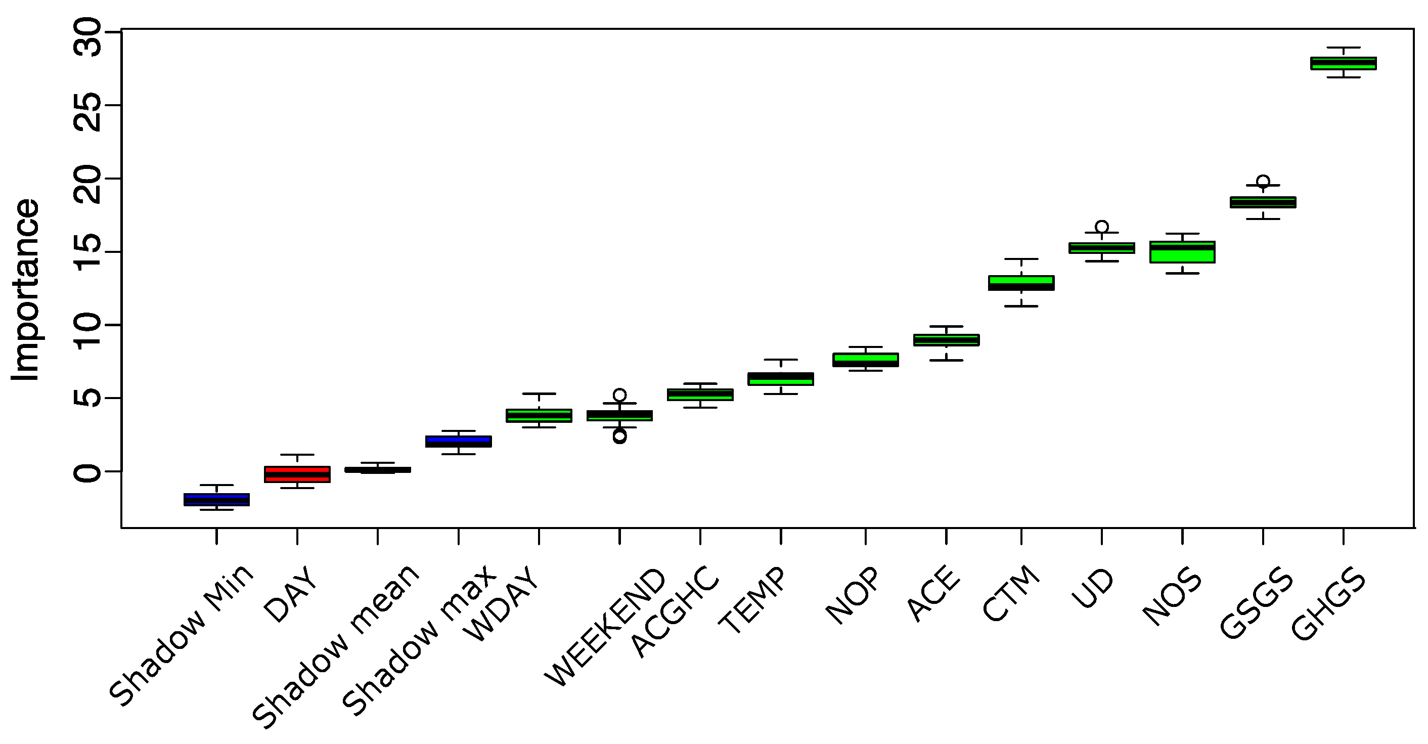
4.3. Feature Importance

The aim of this work is the classification and forecasting of energy consumption depending on the season. However, despite the multiple variables contained in the dataset, there are a certain number of them that contributes most comparing to the rest. Then, to get a better grasp the importance of each variable on the prediction of the energy consumption, we applied the Boruta feature importance algorithm. This method belongs to the wrapper family methods, which are characterized by the evaluation of each subset created using a determined resampling method combined to an ensemble model (in this case, Random Forest). The Boruta algorithm works as follows:

• First, it duplicates the dataset, and rearrange the values in each column. These values are called shadow features. Then, it trains a classifier on the dataset. By this means, this model provides an idea of the importance through the accuracy for each of the features of the dataset. The higher the score, the better or more important.
• Then, the algorithm checks for each of your real features if they are importance. Each feature is evaluated through the Z-score i.e., the number of standard deviations from the mean a data point is. Then, the importance of each feature is depends on whether the feature has a higher score than the maximum score of the shadow features. If they do, they are taken into account. These are called hits. Next, another iteration is performed. After a predefined set of iterations, the algorithm provides with a table of these hits.
• At every iteration, the model compares the Z-scores of the shuffled copies (shadows features) and the original variables to see if the latter outperformed the former. If so, then the algorithm marks the feature as important. In summary, the algorithm validates the importance of the feature by comparing with random shuffled copies, fact that boost up the robustness.

Figure 5 illustrates a boxplot of the ranked predictors using the Boruta algorithm. Blue boxplots correspond to minimal, average and maximum Z score of shadow features. Red and green boxplots represent Z scores of respectively worst and top variance contributors. There, it can be seen that the predictors contributing the most to the variability of the dataset were GHGS, GSGS, NOS, CTM, UD. Most of the predictors have a significant important, as only the variable DAY contributed less than the shadow features. This is the reason why we did not consider this stage as a feature selection one but for enhancing the exploratory analysis above mentioned

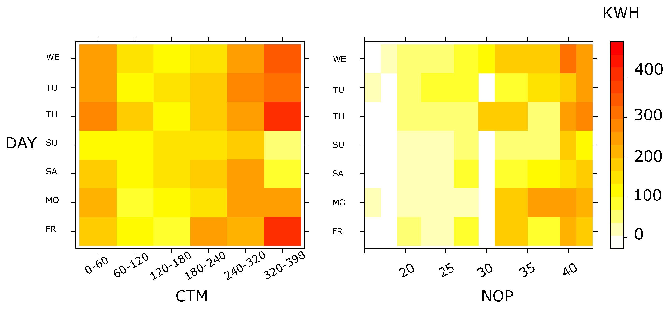
4.4. Analysis per Season

EVs charging behavior depends on several factors such as socio-demographics, time of the day, location of CS, distance travelled, tax incentives [46]. However, along the year, the human being varies their typical activities depending on the season. For instance, in summer the activities for somebody could be different from the activities in winter. These changes affect the driving range of EVs directly due to the strong dependence on the ambient temperature. Most of EVs owners avoid to use their vehicles in winter as sub-zero temperatures may degrade the battery’s pack life expected [47]. Several studies developed have demonstrated that reductions in driving range down to to 45% [48], 34.3% [49], and 31% [50] on extreme cold (under zero degrees) scenarios.

We used the dataset mentioned above to analyze the charging behavior of EVs owners on each season. Figure 6 illustrates a general picture of charging behaviors across seasons from their probability density functions. The season which accounts for significant EV load and charging sessions is autumn. This fact is strongly related to the fact as the ambient temperature begins to decrease, the available battery range gets reduced, and owners may be charging their vehicles more often to ensure they have sufficient range to reach their final destination [16]. Winter represents the lowest energy consumption, and the frequency of small charging sessions are higher than the rest of the seasons. This behavior is explained from several domains, for example, cold temperatures cause drastic changes in human being’s habits, especially during sub-zero temperatures as the Canada, Sweden, Norway and Finland cases [51] were people prefer to stay indoors. This behavior may aid to increase battery’s lifetime, as users do not use their vehicles in the same way as during other seasons, where the ambient temperature is the warmest. Charging habits during Spring and Summer are quite similar. This may be explained by during these seasons, people tend to stay outside the house to take advantage of agreeable weather and longer days (more sunlight hours).

4.5. EVs Charging Load Classification per Season

As mentioned in Section 4.4, the dataset was divided by seasons. We used several classification methods, including the classic ones such as support vector machines with linear (SVML) and radial (SVMR) kernels, linear discriminant analysis (LDA and SLDA), multinomial regression (MN), decision trees (DT), and naive Bayes (NB) and K-neighbors (KNN). In addition, we decided to evaluate models recurrent-based such as extreme gradient boost (XGBOOST) and boosted logistic regression (BLR). Finally, we used Lasso and elastic-net regularized generalized linear models (GLMNET) and bagging trees (TBAG) as ensemble models. These set of classifiers were trained and tested over the unseen (test) data by using a 10-folds cross-validation algorithm.

4.6. Performance Metrics for Classification

In this work, we established accuracy and the receiver operating characteristic (ROC) curve as performance metrics for classification. First, the ROC curve evaluates the performance regarding the number of true positives (TP), true negatives (TN), false positives (FP), false negatives (FN), and area under the curve (AUC) to visualize the detection ability of a model. These metrics were computed during a cross-validation procedure for each model. Below there is a description of the metrics.

4.6.1. Accuracy

It computes the number of TP and TN over the total of observations.

$$Accuracy=\frac{TP+TN}{P+N}$$

4.6.2. Receiver Operating Characteristic

This metric describes the TP percentage versus the FP percentage. It helps to understand how sensitive (TP rate) and specific (TN rate) is a model. The ROC curve can be obtained by plotting the TP rate against FP. The best possible AUC is 1.0. The diagonal line in the ROC depicts randomness.

4.7. EVs Charging Load Prediction

To assess the effectiveness of the prediction the demanda data of all the seasons of Boulder, Colorado were selected as a numerical example for simulation verification. The daily energy demand of EVs users was taken as the outcome, and the accuracy of both RF and QPM was observed. We designed three scenarios to predict the future season from the previous one/ones, as below explained:

• Case I: We used the data from spring (Training) to forecast the data in summer (Test)
• Case II: We joined the data from spring and summer (Training) to forecast the data in autumn (Test)
• Case III: We joined data from spring, summer and autumn (Training), to forecast the data in winter (Test)

4.8. Performance Metrics for Regression

The mean absolute percentage error (MAPE) and the root mean square error (RMSE) were selected as metrics to assess the performance of regression models. They can be computed from the below mentioned equations:

$$\begin{array}{c}\hfill {\displaystyle MAPE=\frac{100\%}{n}\sum _{t=1}^n\left|\frac{\widehat{p_n\left(i\right)}-p_n\left(i\right)}{p_n\left(i\right)}\right|}\end{array}$$

$$\begin{array}{c}\hfill {\displaystyle RMSE=\sqrt{\frac{1}{n}\sum _{t=1}^n\widehat{p_n\left(i\right)}-p_n\left(i\right)}}\end{array}$$

where $p_n\left(i\right)$ and $\widehat{p_n\left(i\right)}$ are the real and predicted values of the ith data, respectively, also n is the length of the data used for verification.

5. Results and Discussion

5.1. Statistical Analysis

The differences among the means in KWH and CTM per season according to ANOVA results had $p<0.05$, which means that there is high compatibility between the statistical model and the data [52]. From Figure 7, we found that although during winter, the load was lower than the rest of the seasons, the charging time in this season was higher in comparison with the rest. The behavior during Summer and Spring is not entirely different. During autumn, the CTM increases but not as much as in winter, when the load demand reaches its maximum value.

Also, Chi-squared tests were conducted to test if the EVs load and charging time categorical variables were related to temporal factors, i.e., day, weekday, weekend. The resulting chi-square values $(\tilde{\chi }=58.317,df=48,p=0.1462)$, $(\tilde{\chi }=20.704,df=6,p=0.007)$, and $(\tilde{\chi }=20.704,df=8,p=0.007)$ respectively, it shows that the Evs load is not related to whether it is Monday, Thursday and so on but it is related to whether Weekday or Weekend. The same procedure was conducted with charging time, and results pointed out that weekdays or weekends do not affect this predictor, $(\tilde{\chi }=6.3759,df=5)$ from p > 0.05.

5.2. Classification

First, the data set was standardized and centered. Then, we divided it into 80% for model training and 20% for testing the model with unseen data. The resulting dataset is not balanced during training and test. Among the twelve (12) models trained and tested, the XGBOOST model is the one that provided better global performance with a mean global accuracy of 99.71% and a mean global AUC of 99.96%. Results are shown in

Table 2. 10-fold cross validation results for each model at several metrics.

Model	Min Acc	Mean Acc	Max Acc	Min AUC	Mean AUC	Max AUC
SVML	0.7058	0.7653	0.8	0.9831	0.9934	1
SVMR	0.8484	0.9236	1	0.9759	0.9868	1
KNN	0.8888	0.9213	1	0.9857	0.9927	1
LDA	0.8529	0.9530	1	0.9452	0.9914	1
STEPLDA	0.9117	0.9530	0.97	0.9930	0.9981	1
MN	0.9393	0.9705	1	0.9975	0.9996	1
NB	0.9142	0.9854	1	0.9912	0.9991	1
DT	0.9696	0.9969	1	0.9773	0.9977	1
XGBTREE	0.9696	0.9969	1	1	1	1
GLMNET	0.9411	0.9822	1	0.9887	0.9997	1
BLR	0.9705	0.9912	1	0.9907	0.9980	1
TBAG	0.9696	0.9969	1	1	1	1

. This table presents information related to the variability of the results across cross-validation folds. From Figure 8, it is clear that all the models provided an acceptable performance to discriminate among seasons. The five models that have the highest performance values are XGBOOST, TBAG, NB, DT, and BLR. However, to get further deep and correctly select the best model, we tested the ability of the twelve trained models to discriminate among season pairs. We realized that the XGBOOST ability to perform the last mentioned task is great, but the GLMNET model provides better performance than the rest. Figure 9 shows the ROC curve for GLMNET. This figure aids to identify the best model able to differentiate among season pairs i.e., Autumn-Spring (AU-SP), Autumn-Summer (AU-SU), and Autumn-Winter (AU-WIN), Spring-Summer (SP-SU), Spring-Winter (SP-WIN), and Summer-Winter (SU-WIN). In the figure, there are four ROC plots, one for each season. In each plot, the current season is the true target to predict. Generally, the model almost always provides more information that the diagonal line which represents the randomness, excepting while discriminating between SU-WIN when the true target is Spring. When the true target was Winter and Autumn, the model can discriminate among all the pairs.

Nevertheless, this could fall in recognizing Summer when the pair is SU-WIN. On the other hand, when the true target is Summer, this model may fail if the season pair is AU-WIN since it is close to the diagonal in the ROC curve.

Table 3. AUC values per season target and model.

Model	Target Season	AUC
GLMNET	WIN	0.9376
	SP	0.8587
	SU	0.8413
	AU	0.9489
XGBOOST	WIN	0.8237
	SP	0.8307
	AU	0.7806
	WIN	0.8082

shows the mean AUC values for each season. Therefore, it can we can state that GLMNET is the best model to classify the charging load stations.

Finally, the information of the GLMNET performance during training and test is presented by their confusion matrices in Figure 10 where the numbers in parentheses represent the observations classified per class. When evaluated on the test data, this model allows to correctly classify seasons with a mean accuracy of 98.78% at 95% confidence interval (93.39–99.97%). During the training stage, it can accurately predict the target seasons with a mean accuracy of 98.24%. Besides, on the test subset, this model has a No Information Rate of 37.8% and a balanced accuracy per class close to 98.56% in all classes.

5.3. Regression

CS’ aggregated data of the above mentioned scenarios were selected as numerical examples to evaluate the performance of the models proposed in Section 2. No features selection techniques were used, and only the continuous variables contained in Table 1 were taken into account. The models were evaluated using a repeated 10-fold cross-validation algorithm. Each model was trained and tested considering each Case described in Section 4.7. For instance, the case I means that the models used the data from spring to forecast the energy consumption in summer, the case II used the data from spring and summer to forecast the demand in fall, and so on.

Regarding QPM, the dispersion parameter for each scenario are 1.4711, 1.7721 and 1.9362, respectively. Since this parameter is higher than one (presence of overdispersion), QPM can be used under such consideration.

Therefore, we used the future season as test sample set and the data from current season/seasons were considered as training sample set. For the first scenario, the number of trees selected to minimize the RMSE was 189. The depth of each tree is fixed at three to avoid overfitting. Figure 11A illustrates the resulting forecast for this scenario. Both models can forecast the demand in Summer from Spring data during the first 60 days. However, QPM (RMSE = 25.66 and MAPE = 1.3822%) tends to fail after that period, and the load prediction overestimate the current value. In contrast, RF (RMSE = 11.65 and MAPE = 0.08%) seems to fit better with the real data.

Figure 11, illustrates the results of the second scenario. Regarding RF, the number of trees selected to minimize the RMSE was 49, and the depth of each tree was fixed at three. QPM (RMSE = 1.80, MAPE = 0.44%) tends to underestimate the real load demand of EVs users. On the contrary, RF (RMSE = 8.82, MAPE = 0.28%) tends to fit better to the current data. Nevertheless, there are some days when the model underestimates the CS’s demand and these days, QPM provides better the real data. Figure 11C shows the results of the last scenario. Overall, both models fit the data. However, once RF (RMSE = 6.68, MAPE = 0.6140%) tends to fit better with the real data. However, the firsts 45 days QPM (RMSE = 12.35, MAPE = 1.0534%) overestimate the demand in comparison with RF. The optimal number of trees to minimize the RMSE was 203, and the depth was fixed at seven.

From these results, it is clear that both RF and QPM are models able to forecast EVs load. However, RF provided better global performance than QPM. On the one hand, QPM often tends to underestimate and overestimate EVs load, and RF tends to adjust better to the variability of the test data. On the other hand, during significant variations in real data, QPM fitted better than RF with the actual data, as was evident during some time intervals in Figure 11B. Several studies have been carried out in this topic, and our results are comparable with them. Lu et al. used RF and support vector regression (SVR) in a case study to forecast the load data of a single charging station in Shenzen. These models were evaluated from RMSE and MAPE metrics. In contrast with their results for prediction of a single station data from 14 June to 26 June (RMSE = 2.27, MAPE = 9.76%), we forecasted EVs load for a more extended period, and we obtained better results regarding MAPE in the worst-case 1.3822%, and from RMSE we obtained comparable results. Besides, Dudek used RF for short-term load forecasting. Our findings are similar to time series based models, including CART and ARIMA. The lowest MAPE value that the author reported was 0.92, which is higher in contrast with the obtained by us (0.08).

6. Conclusions

The main conclusions of this work are listed below:

• This paper shows that EVs’ energy consumption can be forecasted and discriminated from seasons using machine learning tools with high accuracy.
• The statistical analysis proved that the seasonality shapes significantly charging behaviors within a 95% compatibility interval. In winter, the EV load is the lowest and the charging time is the maximum, meanwhile, in fall, the demand reaches its maximum value and the charging time is more moderate than winter but higher than Spring and Summer.
• From forecast results, both models were able to predict EVs load on the established scenarios. However, RF provided better global performance reaching MAPE up to 0.08%, and an RMSE of 2.27.
• Twelve classification models were trained and tested to select the one that maximizes the accuracy and the ROC. All the models showed an acceptable performance during the training and test stage. Despite, GLMNET with ($\alpha =1.00$, $\lambda =0.01$) as final parameters was the method that provided the best classification performance according to mean accuracy and ROC. These results suggest that the seasonality effect powerfully shapes charging behaviors, and this fact is related to our findings from the exploratory analysis carried out that charging time and the temperature are inversely correlated.

The main limitation of this work relies on the fact that the used dataset provides only aggregated information and thus the proposed approach is not able to take short-term decisions such as when to connect or disconnect a specific user to the grid. Nevertheless, this work provided results with high accuracy, which allows medium and long-term planning of power systems. Future works will include an approach more focused on non-aggregated data to characterize more detailed behaviors considering socio-demographic variables such as the share of home-based charging. Such information can create a valuable contribution on the evaluation of differences in counties with more share of single homes versus those with multi-households differ in charging behavior over seasons.

References

1. Ayman, E.R. Toward a Sustainable More Electrified Future: The Role of Electrical Machines and Drives. IEEE Electrif. Mag. 2019, 7, 49–59. [Google Scholar]
2. Wu, G.; Zhang, X.; Dong, Z. Powertrain architectures of electrified vehicles: Review, classification and comparison. J. Frankl. Inst. 2015, 352, 425–448. [Google Scholar] [CrossRef]
3. Guirong, Z.; Henghai, Z.; Houyu, L. The Driving Control of Pure Electric Vehicle. Procedia Environ. Sci. 2011, 10, 433–438. [Google Scholar] [CrossRef] [Green Version]
4. Langbroek, J.H.; Franklin, J.P.; Susilo, Y.O. The effect of policy incentives on electric vehicle adoption. Energy Policy 2016, 94, 94–103. [Google Scholar] [CrossRef]
5. Cozzi, L. World Energy Outlook 2018. In International Energy Agency; Technical Report; IEA: Paris, France, 2019. [Google Scholar]
6. Tamai, G. What Are the Hurdles to Full Vehicle Electrification? [Technology Leaders]. IEEE Electrif. Mag. 2019, 7, 5–11. [Google Scholar] [CrossRef]
7. Mega, V.P. The Paths to Decarbonisation Through Cities and Seas. In Eco-Responsible Cities and the Global Ocean; Springer: Berlin, Germany, 2019; pp. 121–166. [Google Scholar]
8. IEA; UNSD; WHO. Tracking SDG 7: The Energy Progress Report 2019; IRENA: Washington, DC, USA, 2019. [Google Scholar]
9. Anastasiadis, A.G.; Kondylis, G.P.; Polyzakis, A.; Vokas, G. Effects of Increased Electric Vehicles into a Distribution Network. Energy Procedia 2019, 157, 586–593. [Google Scholar] [CrossRef]
10. Haustein, S.; Jensen, A.F. Factors of electric vehicle adoption: A comparison of conventional and electric car users based on an extended theory of planned behavior. Int. J. Sustain. Transp. 2018, 12, 484–496. [Google Scholar] [CrossRef] [Green Version]
11. Hosseini, S.S.; Badri, A.; Parvania, M. A survey on mobile energy storage systems (MESS): Applications, challenges and solutions. Renew. Sustain. Energy Rev. 2014, 40, 161–170. [Google Scholar] [CrossRef]
12. Dominguez, J.; Dante, A.; Agbossou, K.; Henao, N.; Campillo, J.; Cardenas, A.; Kelouwani, S. Optimal Charging Scheduling of Electric Vehicles based on Principal Component Analysis and Convex Optimization. In Proceedings of the 2020 IEEE 29th International Symposium on Industrial Electronics (ISIE), Delft, The Netherlands, 17–19 June 2020; pp. 935–940. [Google Scholar]
13. Shahidinejad, S.; Filizadeh, S.; Bibeau, E. Profile of charging load on the grid due to plug-in vehicles. IEEE Trans. Smart Grid 2012, 3, 135–141. [Google Scholar] [CrossRef]
14. Shao, S.; Pipattanasomporn, M.; Rahman, S. Demand response as a load shaping tool in an intelligent grid with electric vehicles. IEEE Trans. Smart Grid 2011, 2, 624–631. [Google Scholar] [CrossRef]
15. Zhao, Y.; Che, Y.; Wang, D.; Liu, H.; Shi, K.; Yu, D. An optimal domestic electric vehicle charging strategy for reducing network transmission loss while taking seasonal factors into consideration. Appl. Sci. 2018, 8, 191. [Google Scholar] [CrossRef] [Green Version]
16. Boston, D.; Werthman, A. Plug-in Vehicle Behaviors: An analysis of charging and driving behavior of Ford plug-in electric vehicles in the real world. World Electr. Veh. J. 2016, 8, 926–935. [Google Scholar] [CrossRef] [Green Version]
17. Ul-Haq, A.; Azhar, M.; Mahmoud, Y.; Perwaiz, A.; Al-Ammar, E.A. Probabilistic modeling of electric vehicle charging pattern associated with residential load for voltage unbalance assessment. Energies 2017, 10, 1351. [Google Scholar] [CrossRef]
18. Taylor, J.W.; McSharry, P.E. Short-term load forecasting methods: An evaluation based on european data. IEEE Trans. Power Syst. 2007, 22, 2213–2219. [Google Scholar] [CrossRef] [Green Version]
19. Hahn, H.; Meyer-Nieberg, S.; Pickl, S. Electric load forecasting methods: Tools for decision making. Eur. J. Oper. Res. 2009, 199, 902–907. [Google Scholar] [CrossRef]
20. Hong, T.; Xie, J.; Black, J. Global energy forecasting competition 2017: Hierarchical probabilistic load forecasting. Int. J. Forecast. 2019, 35, 1389–1399. [Google Scholar] [CrossRef]
21. Liang, Y.; Niu, D.; Hong, W.C. Short term load forecasting based on feature extraction and improved general regression neural network model. Energy 2019, 166, 653–663. [Google Scholar] [CrossRef]
22. Ganguly, A.; Goswami, K.; Mukherjee, A.; Sil, A.K. Short-Term Load Forecasting for Peak Load Reduction Using Artificial Neural Network Technique. In Advances in Computer, Communication and Control; Springer: Singapore, 2019; pp. 551–559. [Google Scholar]
23. Franke, T.; Krems, J.F. Understanding charging behaviour of electric vehicle users. Transp. Res. Part F Traff. Psychol. Behav. 2013, 21, 75–89. [Google Scholar] [CrossRef]
24. Chen, L.; Nie, Y.; Zhong, Q. A model for electric vehicle charging load forecasting based on trip chains. Trans. China Electrotech. Soc. 2015, 30, 216–225. [Google Scholar]
25. Wang, H.; Wang, B.; Fang, C.; Li, W.; Huang, H. Charging Load Forecasting of Electric Vehicle Based on Charging Frequency. In IOP Conference Series: Earth and Environmental Science; IOP Publishing: Bristol, UK, 2019; p. 062008. [Google Scholar]
26. Gerossier, A.; Girard, R.; Kariniotakis, G. Modeling and Forecasting Electric Vehicle Consumption Profiles. Energies 2019, 12, 1341. [Google Scholar] [CrossRef] [Green Version]
27. Alegre, S.; Míguez, J.V.; Carpio, J. Modelling of electric and parallel-hybrid electric vehicle using Matlab/Simulink environment and planning of charging stations through a geographic information system and genetic algorithms. Renew. Sustain. Energy Rev. 2017, 74, 1020–1027. [Google Scholar] [CrossRef]
28. Mao, D.; Tan, J.; Liu, G.; Wang, J. Location Planning of Fast Charging Station considering its Impact on the Power Grid Assets. arXiv 2019, arXiv:1903.10149. [Google Scholar]
29. Zhang, H.; Hu, Z.; Song, Y.; Xu, Z.; Jia, L. A prediction method for electric vehicle charging load considering spatial and temporal distribution. Autom. Electr. Power Syst. 2014, 38, 13–20. [Google Scholar]
30. Ahmad, A.; Hassan, M.; Abdullah, M.; Rahman, H.; Hussin, F.; Abdullah, H.; Saidur, R. A review on applications of ANN and SVM for building electrical energy consumption forecasting. Renew. Sustain. Energy Rev. 2014, 33, 102–109. [Google Scholar] [CrossRef]
31. Jiao, R.; Zhang, T.; Jiang, Y.; He, H. Short-Term Non-Residential Load Forecasting Based on Multiple Sequences LSTM Recurrent Neural Network. IEEE Access 2018, 6, 59438–59448. [Google Scholar] [CrossRef]
32. Abbasi, R.A.; Javaid, N.; Ghuman, M.N.J.; Khan, Z.A.; Rehman, S.U. Short Term Load Forecasting Using XGBoost. In Workshops of the International Conference on Advanced Information Networking and Applications; Springer: Berlin, Germany, 2019; pp. 1120–1131. [Google Scholar]
33. Yan, D.; O’Brien, W.; Hong, T.; Feng, X.; Gunay, H.B.; Tahmasebi, F.; Mahdavi, A. Occupant behavior modeling for building performance simulation: Current state and future challenges. Energy Build. 2015, 107, 264–278. [Google Scholar] [CrossRef] [Green Version]
34. Khatoon, S.; Singh, A.K. Effects of various factors on electric load forecasting: An overview. In Proceedings of the 2014 6th IEEE Power India International Conference (PIICON), Delhi, India, 5–7 December 2014; pp. 1–5. [Google Scholar]
35. Amara, F.; Agbossou, K.; Dubé, Y.; Kelouwani, S.; Cardenas, A. Estimation of temperature correlation with household electricity demand for forecasting application. In Proceedings of the IECON 2016—42nd Annual Conference of the IEEE Industrial Electronics Society, Florence, Italy, 23–26 October 2016; pp. 3960–3965. [Google Scholar]
36. Rijal, H.; Humphreys, M.; Nicol, F. Adaptive thermal comfort in Japanese houses during the summer season: Behavioral adaptation and the effect of humidity. Buildings 2015, 5, 1037–1054. [Google Scholar] [CrossRef]
37. Wang, X.; Zhang, M.; Ren, F. Learning customer behavior for effective load forecasting. IEEE Trans. Knowl. Data Eng. 2018, 31, 938–951. [Google Scholar] [CrossRef]
38. Wang, D.; Sun, Z. Big data analysis and parallel load forecasting of electric power user side. Proc. CSEE 2015, 35, 527–537. [Google Scholar]
39. Wu, X.; He, J.; Zhang, P.; Hu, J. Power system short-term load forecasting based on improved random forest with grey relation projection. Autom. Electr. Power Syst. 2015, 39, 50–55. [Google Scholar]
40. Dudek, G. Short-term load forecasting using random forests. In Intelligent Systems’ 2014; Springer: Berlin, Germany, 2015; pp. 821–828. [Google Scholar]
41. Electric Vehicle Charging Stations: Energy Consumption & Savings. Available online: https://bouldercolorado.gov/open-data/electric-vehicle-charging-stations/ (accessed on 16 May 2020).
42. Colorado Energy Office. Colorado Energy Office Annual Report 2017–2018; Technical report; Colorado Energy Office: Denver, CO, USA, 2015.
43. Toor, W.; Salisbury, M. Boulder Electric Vehicle Infrastructure and Adoption Assessment. In Southwest Energy Efficiency Project; Technical report; Southwest Energy Efficiency Project (SWEEP): Denver, CO, USA, 2015. [Google Scholar]
44. Colorado Energy Office. Colorado’s electric vehicle roadmap. In Regional Air Quality Council; Technical report; Colorado Energy Office: Denver, CO, USA, 2020. [Google Scholar]
45. Dowds, J.; Hines, P.; Farmer, C.; Watts, R.; Letendre, S. Plug-in Hybrid Electric Vehicle Research Project: Phase Two Report; Technical report; UVM Transportation Research Center: Burlington, VT, USA, 2010. [Google Scholar]
46. Vassileva, I.; Campillo, J. Adoption barriers for electric vehicles: Experiences from early adopters in Sweden. Energy 2017, 120, 632–641. [Google Scholar] [CrossRef]
47. Jaguemont, J.; Boulon, L.; Dubé, Y. A comprehensive review of lithium-ion batteries used in hybrid and electric vehicles at cold temperatures. Appl. Energy 2016, 164, 99–114. [Google Scholar] [CrossRef]
48. Meyer, N.; Whittal, I.; Christenson, M.; Loiselle-Lapointe, A. The impact of driving cycle and climate on electrical consumption and range of fully electric passenger vehicles. In Proceedings of the EVS26 International Battery, Hybrid, and Fuel Cell Electric Vehicle Symposium, Los Angeles, CA, USA, 6–9 May 2012; pp. 1–11. [Google Scholar]
49. Reyes, J.R.M.D.; Parsons, R.V.; Hoemsen, R. Winter happens: The effect of ambient temperature on the travel range of electric vehicles. IEEE Trans. Veh. Technol. 2016, 65, 4016–4022. [Google Scholar] [CrossRef]
50. How Do Extremely Cold Temperatures Affect the Range Of An Electric Car? Available online: https://www.fleetcarma.com/electric-car-range-in-bitter-cold/ (accessed on 16 December 2013).
51. Sovacool, B.K.; Noel, L.; Kester, J.; de Rubens, G.Z. Reviewing Nordic transport challenges and climate policy priorities: Expert perceptions of decarbonisation in Denmark, Finland, Iceland, Norway, Sweden. Energy 2018, 165, 532–542. [Google Scholar] [CrossRef] [Green Version]
52. Wasserstein, R.L.; Schirm, A.L.; Lazar, N.A. Moving to a World Beyond “p < 0.05”. Am. Stat. 2019, 73, 1–19. [Google Scholar]
Figure 1. Charging stations distribution in the city.
Sustainability 12 07769 g001
Figure 2. Energy consumption changes along the year.
Sustainability 12 07769 g002
Figure 3. Exploratory analysis based on principal components for the data provided by Markram.
Sustainability 12 07769 g003
Figure 4. EV load heatmap from charging intervals and number of ports used diary.
Sustainability 12 07769 g004
Figure 5. Feature importance in the prediction of energy consumption using the Boruta algorithm.
Sustainability 12 07769 g005
Figure 6. Density plot for energy consumption per session.
Sustainability 12 07769 g006
Figure 7. ANOVA results for CTM and KWH depending on the season.
Sustainability 12 07769 g007
Figure 8. Boxplot for the cross-validation results of both metrics selected.
Sustainability 12 07769 g008
Figure 9. GLMNET AUC during cross-validation.
Sustainability 12 07769 g009
Figure 10. Confusion matrices for training and test.
Sustainability 12 07769 g010
Figure 11. Load CS forecast for seasons: (A) Summer from Spring; (B) Autumn from Spring+Summer; and (C) Winter from the whole seasons altogether.
Sustainability 12 07769 g011