Liner Shipping Schedule Design for Near-Sea Routes Considering Big Customers’ Preferences on Ship Arrival Time

Abstract

There usually exist a few big customers at ports of near-sea container shipping routes who have preferences on the weekly ship arrival times due to their own production and sale schedules. Therefore, in practice, when designing ship schedules, carriers must consider such customers’ time preferences, regarded as weekly soft-time windows, to improve customer retention, thereby achieving sustainable development during a depression in the shipping industry. In this regard, this study explores how to balance the tradeoff between the ship total operating costs and penalty costs from the violation of the weekly soft-time windows. A mixed-integer nonlinear nonconvex model is proposed and is further transformed into a mixed-integer linear optimization model that can be efficiently solved by extant solvers to provide a global optimal solution. The proposed model is applied to a near-sea service route from China to Southeast Asia. The results demonstrate that the time preferences of big customers affect the total cost, optimal sailing speeds, and optimal ship arrival times. Moreover, the voyage along a near-sea route is generally short, leaving carriers little room for adjusting the fleet size.

1. Introduction

The global maritime trade has lost momentum in recent years owing to a series of downside risks such as Sino-US trade friction. The trade volume expanded by 2.7% in 2018, which was not only lower than the 4.1% growth rate in 2017, but also lower than the historical average of 3.0%. The growth rate in containerized global ports throughput decreased from 6.7% in 2017 to 4.7% in 2018 [1]. The implementation of the global sulfur cap in January 2020 increased operating costs and may also lead to the loss of some market share to land-based modes [2,3]. Facing this situation, container lines have adopted strategies such as slow steaming and route layout optimization to reduce operating costs and enhance profitability as well as to realize transportation sustainability. In addition to the above measures, designing schedules that comply with the requirements of big customers, such as freight forwarders and large factories, to alleviate customer loss and enhance customer satisfaction is also important for container lines.

In the near-sea routes in the Asian region, a considerable number of ports can be identified with large freight forwarders or factories with a single type of good and large shipments. According to our survey, the shipments from a big customer may account for 50%, or even more than 80%, of the shipments at the local port on the route. Both fruits and waste plastics shipped to China from some ports in Southeast Asia and secondhand cars transferred from Nagoya in Japan to Central Asia via Lianyungang illustrate the findings of our survey. Sometimes, shipping lines may even add a call for some big customers. For example, SITC container lines (SITC) added a call to Hitachinaka on Mondays on its CJV6 service in 2015 to accommodate Toyota’s shipment demand. Considering their own production and/or sale schedules as well as the pressure of product inventory, these big customers generally have a preference for the weekly day on which the ship arrives at the loading ports. During a depression in the shipping industry, the sustainability of long-term partnerships with big customers cannot be neglected. Therefore, a few adjustments should be made in the shipping schedules to address the time preferences of the shipping demands. The preferences of the big customers for the ship arrival time at these ports can be regarded as weekly soft-time windows. The service can also start outside this time window if an appropriate penalty is paid. The penalty involves the lost cost of goodwill, sales, and service satisfaction owing to customer inconvenience [4]. We use the term “port soft-time windows” to indicate the ship arrival time at the loading ports expected by the big customers.

Different shipping schedules mean different sailing times on shipping legs, and thus, different sailing speeds. Despite their relatively small number in the world fleet, containerships are the largest maritime CO₂ emitters [5]. Because emissions are directly proportional to bunker consumption, sailing speed is closely related to the environmental dimension of shipping [6]. Lowering speed can reduce ship emissions, thereby reducing environmental impact [7]. Therefore, the schedule design affects the bunker consumption and air pollutant emissions.

In addition, providing a shorter shipping time for containers from origin to destination can improve the market competitiveness of container lines [8]; however, it also leads to a higher bunker consumption as well as higher air pollutant emissions. Meanwhile, a longer shipping time leads to less bunker consumption and air pollutant emissions, which are conducive to the sustainable development of the environment. In summary, when designing the shipping schedule, container lines must balance the tradeoff between the vessel’s operating cost, fuel cost, and penalty costs associated with the port soft-time windows and shipping time. This study provides decision support to help container lines cope with smaller profit margins as a result of a slacking shipping market demand.

2. Literature Review

Ship scheduling problems are the focus of this study; this research topic has been covered in a few survey papers, for example, Christiansen et al. [9], Meng et al. [10], Psaraftis and Kontovas [6], Tran and Haasis [11], Wang and Meng [12], and Lee and Song [13]. In container liner shipping, the ship scheduling problem is a tactical-level decision problem made every three to six months [9]. Ship scheduling generally involves speed optimization and/or designs of arrival and departure times for given shipping routes. The schedules and speeds are highly correlated because once the schedules are determined, the speeds are roughly determined.

Ship speed optimization is incorporated into the network design in some studies, in which the average ship sailing speed is simply used when calculating the voyage time. Agarwal and Ergun [14] were the first to consider the weekly frequency constraint for ship scheduling and cargo routing problems in the liner shipping network design. Shintani et al. [15] designed a single shipping route considering empty container repositioning using a genetic algorithm-based heuristic. Wang and Meng [16] examined the liner shipping network design problem considering the delivery deadline in which the actual transit time from an origin port to a destination port could not exceed its corresponding deadline. In contrast to most studies on network design, Wang et al. [17] directly optimized the ship sailing speed by treating it as a decision variable during model formulation. Kim et al. [18] designed a simple single route by considering the variable sailing speed for each leg and the fleet size with the objective of maximizing the carrier’s profit. Koza et al. [19] proposed a mixed-integer programming model for the integrated liner shipping network design and scheduling problem incorporating transshipment times, along with a solution method based on column generation.

With regard to the ship scheduling problem for given service routes, speed optimization is either explicit or implicit in the proposed models and is sometimes incorporated into the fleet deployment problem. A few studies have also examined the container ship scheduling problem considering the uncertainty at ports, for example, Qi and Song [20] and Song et al. [21]. Notteboom and Vernimmen [22] proposed a cost model for simulating the impact of high fuel costs and described how shipping lines change sailing speed and fleet size with high fuel costs. Ronen [23] provided an analysis of the relationship between bunker price, service frequency, sailing speed, and fleet size and developed a cost model to minimize the annual operating cost for a given ship route. Cheaitou and Cariou [24] optimized the sailing speed under a semi-elastic demand. Meng and Wang [25] optimized the operating strategy to simultaneously determine the sailing speed, service frequency, and fleet deployment plan for a single Asia–Europe route. Wang and Meng [26] developed a mixed-integer linear programming model for the fleet deployment problem in which container transshipment operations were allowed at any port. Wang and Meng [27] calibrated the relationship between bunker consumption and sailing speed for container ships using the historical operating data of a global container line. They then formulated a mixed-integer programming model by optimizing the sailing speed of each leg and the number of ships deployed in a liner shipping network while considering container transshipment and routing. Kontovas and Psaraftis [28] examined the operational scenario of speed reduction to reduce bunker consumption and curb emissions, and they discussed two possible ways to decrease time in port: Reducing the port service time and enabling the prompt berthing once containerships arrive. Xia et al. [29] jointly optimized fleet deployment, cargo allocation, and sailing speed for each leg for a network design in which the range of possible speeds is discretized. Du et al. [30] presented a liner ship fleet deployment problem considering collaborative transportation. The problem is formulated as a mixed-integer linear programming model that is solved using CPLEX. Zhen et al. [31] presented an integrated planning model to jointly determine the fleet size, ship schedule, sailing speed per leg, and cargo allocation for a given shipping network with multiple routes. Sheng et al. [32] addressed the joint optimization of ship sailing speed and fleet size for an industrial shipping service operating through the emission control areas. Fan et al. [33] proposed a genetic simulated annealing algorithm for the problem of multi-type tramp ship scheduling and speed optimization by considering carbon emissions. Yang et al. [34] proposed a speed optimization model for a fixed ship route incorporating the influence of ocean currents with the target of minimizing the total fuel consumption. Psaraftis [35] examined reduced speed options, such as imposing a speed limit and imposing a bunker levy, and concluded that market-based measures, such as the bunker levy option, are more beneficial than the speed-limit option for reducing greenhouse gas emissions. Giovannini and Psaraftis [36] developed a profit maximization model for a fixed liner shipping route. Rather than the standard assumption of weekly service frequency, they considered flexible service frequencies that can be selected among a broad set, which is different from most studies on liner shipping. They also examined the impact of the carrier’s decisions on CO₂ emissions.

There are also some studies on ship scheduling associated with fleet deployment in Roll-on Roll-off (Ro-Ro) shipping, for example, Fagerholt et al. [37] and Andersson et al. [38]. Patricksson et al. [39] presented a two-stage stochastic model for the maritime fleet renewal problem and explored various alternatives to cope with the stricter emission regulations. Fischer et al. [40] proposed a mixed-integer linear programming for the fleet deployment problem, together with a set of robust planning strategies for handling disruptions.

Because the daily service capacity of a port is limited, there is no guarantee that a ship can be serviced as soon as it arrives at the port. As a result, the availability of ports, that is, a port-time window, is considered in a few studies. Christiansen and Fagerholt [41] treated the time windows as multiple time windows because they assumed that ports were closed for service at night and during weekends. To avoid idle times in the ports during weekends, a penalty cost was imposed for arrivals at risky times. De et al. [42] studied the ship routing and scheduling problem with multiple time windows for tramp ships, in which a penalty cost was imposed due to delays. Their model incorporated carbon emissions and slow steaming. Kim et al. [43] dealt with the sailing speed optimization problem of tramp shipping with multiple hard-time windows for each port call via an exact algorithm. Aydin et al. [44] considered the waiting costs of early arrivals in the sailing speed optimization problem with time windows on a single voyage. Hvattum et al. [45] developed an exact algorithm to optimize the sailing speed for a fixed sequence of port calls with hard-time windows. They proved that optimal speeds can be obtained in quadratic time. Wang et al. [46] discussed a liner shipping route schedule design problem while considering the availability of ports. They viewed the availability of each port as a hard-time window. Wang et al. [47] examined the same problem by incorporating the availability of each berth at each port, and a mixed-integer nonlinear nonconvex optimization model was formulated to minimize the vessel operating, bunker, and inventory costs. Both Wang et al. [46] and Wang et al. [47] focused on a single shipping route. Alharbi et al. [48] further extended the two previous studies [46,47] to a liner shipping network. In this model, a premium berth with a high penalty could be used when violating the berth time window. However, their model did not consider inventory costs. Dulebenets [49] studied the vessel scheduling problem with a heterogeneous fleet and considered late arrival penalties outside the time windows.

The time windows mentioned in the above ship scheduling articles refer to the reserved time period that a port allocates to serve the ship. Very few studies have addressed the ship scheduling problem by considering the time windows for servicing customers. Fagerholt [4] was the first to raise the issue of soft-time windows in tramp shipping scheduling in which a penalty cost for servicing customers outside the time window was imposed. Yu et al. [50] studied the sailing speed optimization problem with a fuzzy-time window for tramp ships. They used the fuzzy-time window to describe the shipper’s satisfaction. A bi-objective model was formulated to minimize the carrier’s operating cost and the shipper’s satisfaction simultaneously. Both studies are in the field of tramp shipping.

To summarize, existing studies seldom incorporated the big customers’ preferences on ship arrival time when designing liner shipping schedules. This is reflected in the fact that penalties on early arrivals are often neglected. In addition, the port soft-time windows are periodic in this study, which is different from those in tramp shipping. Moreover, rather than considering the market-level shipping times as a benchmark to measure the impact of the designed shipping times, most studies only incorporate inventory costs. In practice, a shorter shipping time can improve customer satisfaction and consequently reduce the total operating cost.

This study aims to design the optimal schedule at each port of call on a shipping route. This design is realized while minimizing the total cost, which is sum of the vessel operating cost, fuel cost, penalty cost associated with the port soft-time windows, and penalty cost for the longer shipping time, minus the bonus for the shorter shipping time. This problem is of practical significance to container lines operating near-sea routes or some feeder routes; the problem can help container lines improve service levels for big customers, thereby enhancing the sustainability in liner shipping networks, environments, and society.

The contribution of this study is threefold. First, the factor of weekly soft-time windows based on the preference of big customers is considered in the liner shipping schedule design problem. Second, a tailored mixed-integer programming model is developed to obtain the optimal shipping schedule. Finally, from the case studies, we can obtain useful management insights that can provide support for container lines.

3. Problem Description

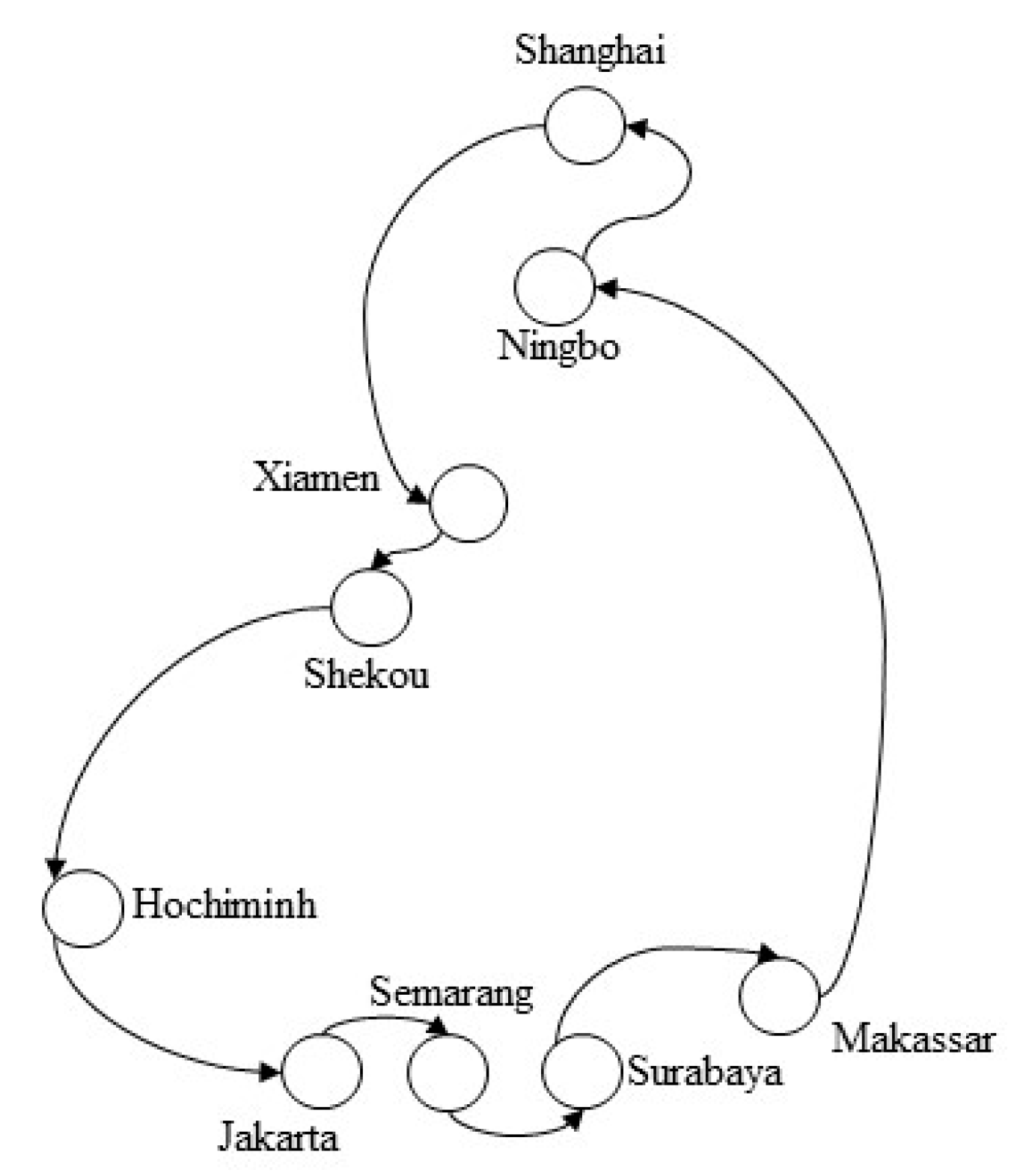
This study considers a typical near-sea shipping route, such as the China-Vietnam-Indonesia (CVI) service operated by SITC container lines in Figure 1, which includes $I=:\left\{1,2,\dots ,N\right\}$ ports of call. The port rotation of the CVI service can be expressed as follows: 1(Ningbo)-2(Shanghai)-3(Xiamen)-4(Shekou)-5(Hochiminh)-6(Jakarta)-7(Semarang)-8(Surabaya)-9(Makassar)-1(Ningbo). The voyage from the $i\mathrm{th}$ to the $\left(i+1\right)\mathrm{th}$ port of call is called leg $i$. We define leg $N$ as the voyage from the $N\mathrm{th}$ port of call back to the first one.

In practice, liner shipping companies generally maintain a weekly service frequency for ports in the service. Therefore, this study considers the total cost of the route in one week.

3.1. Vessel Operating Cost and Shipping Schedule

Let $L_i$ be the distance from the $i\mathrm{th}$ port of call to the $\left(i+1\right)\mathrm{th}$ port of call, and let $v_i$ be the sailing speed on $L_i$. We define the time 00:00 on Sunday as 00:00. Let $t_i^a$ be the ship arrival time at the $i\mathrm{th}$ port of call, and let $t_i^w$ be the fixed dwelling time at the $i\mathrm{th}$ port of call. We assume that berths are available at the actual time of arrival. Then, we can obtain the relation

$$t_{i+1}^a=t_i^a+t_i^w+\frac{L_i}{v_i},\hspace{1em}\hspace{1em}i\in I$$

(1)

We assume that the vessel fleet is homogeneous, and $m$ is the number of ships deployed on the shipping route. To maintain a weekly service frequency, the container lines need to satisfy the following requirements:

$$t_{N+1}^a=t_1^a+168m,$$

(2)

where 168 is the number of hours in a week, and $t_{N+1}^a$ is the time when the ship returns to the first port of call. Let $C^{op}$ represent the fixed weekly operating cost in US dollars per week per ship, including the maintenance cost of ships, the crew’s wages, and port charges. Therefore, the fixed weekly operating cost of the route is $C^{op}m$.

3.2. Port Soft-Time Windows

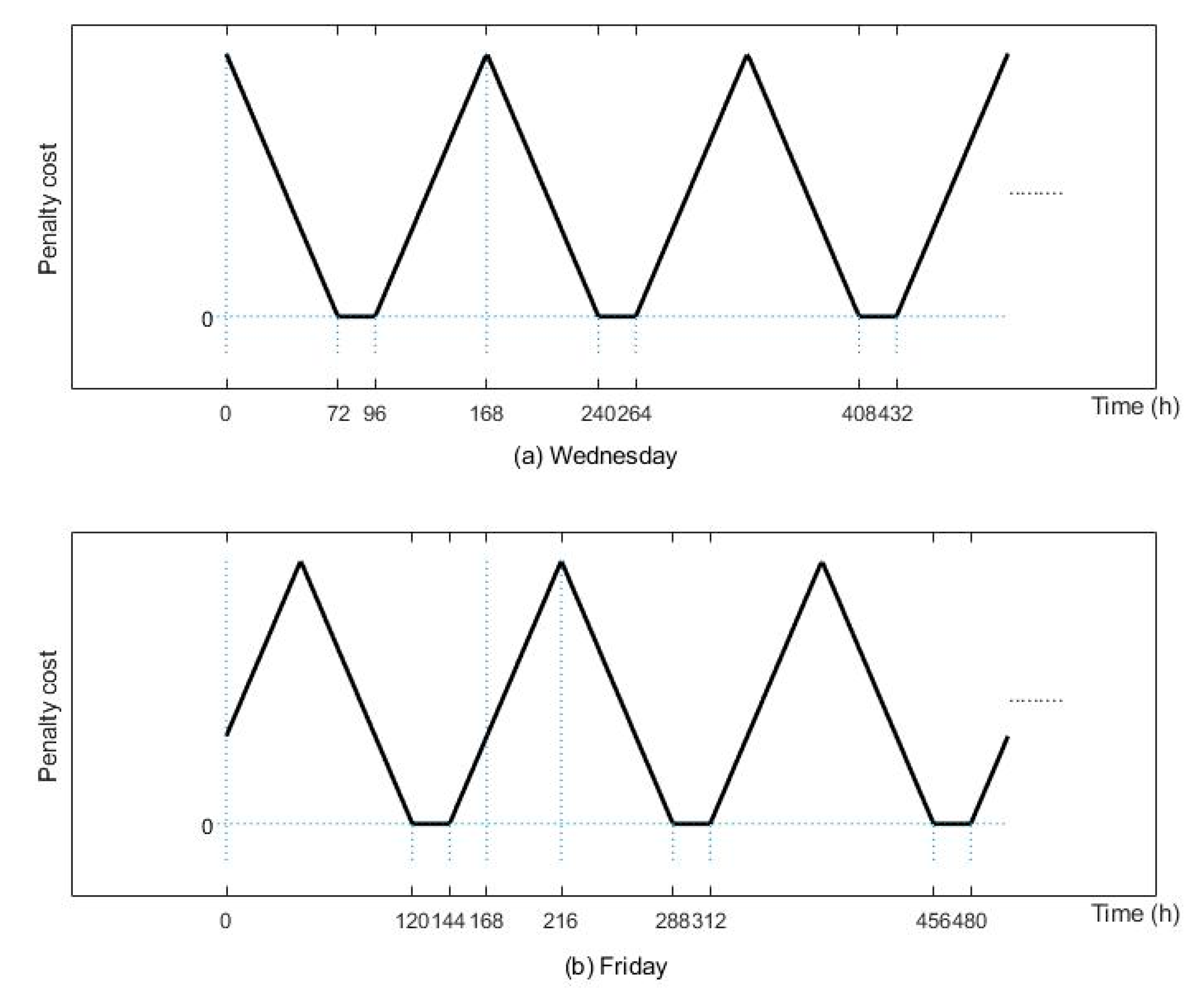
A big customer has preferences for the weekly ship arrival time at the loading port; therefore, when the ship fails to arrive at the port within the time window expected by that customer, a certain penalty must be imposed according to the length of the violation time. Here, we assume that each big customer’s preference for the arrival time is only one day a week. When the customer selects time preferences on two consecutive days or more, the proposed model can be applied after minor modifications. We also define the slope of the penalty function to be the same on both sides. The reason is that this function describes the shipper’s preference on the arrival date, and the less the actual arrival time deviates from this preference, the better. Owing to the characteristics of a weekly service frequency of liner shipping, the soft-time windows are multiply periodic. For example, as shown in Figure 2a, we assume that the time window expected by the customer is Wednesday, that is, the periods between the 72nd and 96th hours, the 240th and 264th hours, and the 408th and 432nd hours, etc. There is no penalty when the ship arrives at the port within these periods. The penalties incurred at the same time in different weeks are the same. For example, the penalty for the ship arriving at the port at $t_i^a=228$ is the same as that for $t_i^a=60$ ($228\mathrm{mod}168=60$). A big customer at each port has a different requirement for the weekly time window; and, the penalty function for each day of the week is different. For example, Figure 2b is the penalty function image for Friday, which can be obtained by shifting the time window image for Wednesday on the time axis.

Let ${\widehat{t}}_i^a$ denote the arrival time of the ship at port of call $i$ in the first week, namely ${\widehat{t}}_i^a=t_i^a\mathrm{mod}168$, and let $p_3\left({\widehat{t}}_i^a\right)$ denote the penalty function for Wednesday as the preferred day at port of call $i$. Then, we have

$$p_3\left({\widehat{t}}_i^a\right)=\{\begin{array}{cc}{\alpha }_i\left(72-{\widehat{t}}_i^a\right),& 0\le {\widehat{t}}_i^a<72\\ 0,& 72\le {\widehat{t}}_i^a\le 96\\ {\alpha }_i\left({\widehat{t}}_i^a-96\right),& 96<{\widehat{t}}_i^a\le 168\end{array},$$

(3)

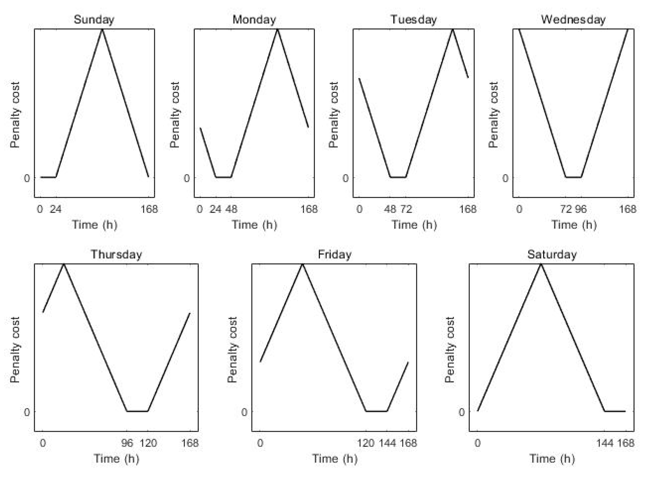
where ${\alpha }_i$ (USD/h) is the unit penalty cost for arriving at the port of call $i$ earlier or later than the expected time of the customer. Since the penalty function for each day of the week is different, the soft-time windows for each day in the first week are shown in Figure 3.

We assume that $p_0\left({\widehat{t}}_i^a\right),\dots ,p_6\left({\widehat{t}}_i^a\right)$ represent the penalty functions of the soft-time windows from Sunday to Saturday at port of call $i$. Then, we have

$$\begin{gathered} p_0\left({\widehat{t}}_i^a\right)=\{\begin{array}{cc}0,& 0\le {\widehat{t}}_i^a\le 24\\ {\alpha }_i\left({\widehat{t}}_i^a-24\right),& 72<{\widehat{t}}_i^a\le 96\\ {\alpha }_i\left(168-{\widehat{t}}_i^a\right),& 96<{\widehat{t}}_i^a\le 168\end{array}{p}_1\left({\widehat{t}}_i^a\right)=\{\begin{array}{cc}{\alpha }_i\left(24-{\widehat{t}}_i^a\right),& 0\le {\widehat{t}}_i^a\le 24\\ 0,& 24<{\widehat{t}}_i^a\le 48\\ {\alpha }_i\left({\widehat{t}}_i^a-48\right),& 48<{\widehat{t}}_i^a\le 120\\ {\alpha }_i\left(192-{\widehat{t}}_i^a\right),& 120<{\widehat{t}}_i^a\le 168\end{array} \\ {p}_2\left({\widehat{t}}_i^a\right)=\{\begin{array}{cc}{\alpha }_i\left(48-{\widehat{t}}_i^a\right),& 0\le {\widehat{t}}_i^a\le 48\\ 0,& 48<{\widehat{t}}_i^a\le 72\\ {\alpha }_i\left({\widehat{t}}_i^a-72\right),& 72<{\widehat{t}}_i^a\le 144\\ {\alpha }_i\left(216-{\widehat{t}}_i^a\right),& 144<{\widehat{t}}_i^a\le 168\end{array}{p}_4\left({\widehat{t}}_i^a\right)=\{\begin{array}{cc}{\alpha }_i\left({\widehat{t}}_i^a+48\right),& 0\le {\widehat{t}}_i^a\le 24\\ {\alpha }_i\left(96-{\widehat{t}}_i^a\right),& 24<{\widehat{t}}_i^a\le 96\\ 0,& 96<{\widehat{t}}_i^a\le 120\\ {\alpha }_i\left({\widehat{t}}_i^a-120\right),& 120<{\widehat{t}}_i^a\le 168\end{array} \\ {p}_5\left({\widehat{t}}_i^a\right)=\{\begin{array}{cc}{\alpha }_i\left({\widehat{t}}_i^a+24\right),& 0\le {\widehat{t}}_i^a\le 48\\ {\alpha }_i\left(120-{\widehat{t}}_i^a\right),& 48<{\widehat{t}}_i^a\le 120\\ 0,& 120<{\widehat{t}}_i^a\le 144\\ {\alpha }_i\left({\widehat{t}}_i^a-144\right),& 144<{\widehat{t}}_i^a\le 168\end{array}{p}_6\left({\widehat{t}}_i^a\right)=\{\begin{array}{cc}{\alpha }_i{\widehat{t}}_i^a,& 0\le {\widehat{t}}_i^a\le 72\\ {\alpha }_i\left(144-{\widehat{t}}_i^a\right),& 72<{\widehat{t}}_i^a\le 144\\ 0,& 144<{\widehat{t}}_i^a\le 168\end{array} \end{gathered}$$

(4)

We define $S:=\left\{0,1,2,3,4,5,6\right\}$ to be a set of all days in a week. Let $x_{is}$ be a binary coefficient that takes a value of 1 if the soft-time window at port of call $i$ is day $s$ or 0 otherwise. Thus, the penalty cost of soft-time windows at the port of call $i$ is ${\displaystyle \sum }_{s\in S}{x}_{is}{p}_s\left({\widehat{t}}_i^a\right)$. For example, if the time preference of a big customer at port 1 is Tuesday, we have $x_{12}=1$ and $x_{10}=x_{11}=x_{13}=x_{14}=x_{15}=x_{16}=0$. This means that the penalty function for port 1 should use the third function in Equation (4), which corresponds to the third image in Figure 3.

The total penalty costs of soft-time windows at all ports of call on the route are as follows:

$${\displaystyle \sum }_{i\in N}{\displaystyle \sum }_{s\in S}{x}_{is}{p}_s\left({\widehat{t}}_i^a\right)$$

(5)

3.3. Shipping Time

We define $h$ to be the weekly container shipping demand corresponding to one O-D port pair and $H$ to be the set of all shipping demands. Let $t_h^{flow}$ represent the total shipping time of container shipping demand $h$ from the loading port to the discharging port, including the sailing time for shipping legs and the fixed dwelling time at ports. Then, we have

$$t_h^{flow}={{\displaystyle \sum }}_{i\in I}{\mu }_{hi}\left(\frac{L_i}{v_i}+t_i^w\right),$$

(6)

where ${\mu }_{hi}$ is a binary coefficient that takes a value of 1 if container shipping demand $h$ is transported on leg $i$ and visits the $i\mathrm{th}$ port of call or 0 otherwise, and $t_i^w$ is the fixed dwelling time at port of call $i$. Let ${\tilde{\gamma }}_h$ represent the unit penalty cost of a shipping time longer than the market-level shipping time corresponding to container shipping demand $h$ (in US dollars per TEU per hour), and let ${\overline{\gamma }}_h$ represent the unit bonus of a shipping time shorter than the market-level shipping time corresponding to container shipping demand $h$ (in US dollars per TEU per hour). Let $T_h$ be the market-level shipping time of the O-D port pair corresponding to container shipping demand $h$, and let $q_h$ be the volume of container shipping demand $h$ (in TEUs). Thus, the bonus or penalty cost of the shipping time with regard to container shipping demand $h$ is as follows:

$$c_h\left(t_h^{flow}\right)=q_h\left({\tilde{\gamma }}_h\max \left\{0,t_h^{flow}-T_h\right\}-{\overline{\gamma }}_h\max \left\{0,T_h-t_h^{flow}\right\}\right)$$

(7)

3.4. Fuel Cost

Let $f_i\left(v_i\right)$ be the bunker consumption in tons per nautical mile at sailing speed $v_i$ on leg $i$. In this study, we assume that $f_i\left(v_i\right)$ is a convex function of $v_i$ [6,27,51]. Then, we have

$$f_i\left(v_i\right)={\delta }_i{\left(v_i\right)}^{b_i},\hspace{1em}{\delta }_i>0,b_i\ge 2,$$

(8)

where ${\delta }_i$ and $b_i$ are two coefficients estimated from practical data. Let $\beta$ be the bunker price in US dollars per ton; thus, the weekly fuel cost on the shipping route is

$$\beta {\displaystyle \sum }_{i\in I}{L}_i{\delta }_i{\left(v_i\right)}^{b_i}$$

(9)

3.5. Mathematical Model

The optimal arrival time of each port of call on the route and the optimal number of ships deployed on the route is determined to minimize the total cost. These values are determined using the liner shipping schedule design problem considering the big customers’ preferences for ship arrival time. First, we list the variables and parameters of the model.

Variables:

$v_i$

Sailing speed of container ship on leg $i$

$m$

Integer variable representing the number of ships deployed on the shipping route

$t_i^a$

Ship arrival time at the $i\mathrm{th}$ port of call.

$t_{N+1}^a$

The time the ship returns to the first port of call after visiting all ports of call for a round-trip journey

${\widehat{t}}_i^a$

Arrival time of ship at port of call $i$ in the first week

$t_h^{flow}$

Total shipping time of container shipping demand $h$ from the loading port to the discharging port

Parameters:

$I$

Set of ports of call

$N$

Number of call ports on the shipping route

$H$

Set of all container shipping demands on the shipping route

$L_i$

Distance from the $i\mathrm{th}$ to the $\left(i+1\right)\mathrm{th}$ port of call

$V_i^{\min }$

Minimum sailing speed of container ship on leg $i$

$V_i^{\max }$

Maximum sailing speed of container ship on leg $i$

$t_i^w$

Dwelling time a ship spends at the $i\mathrm{th}$ port of call.

$C^{op}$

Weekly operating cost of the container ship

$S$

Set of all days in a week.

${\alpha }_i$

Unit penalty cost for arriving at port of call $i$ earlier or later than the expected time of the customer

$x_{is}$

Binary coefficient, which equals 1 if and only if the soft-time window at port of call $i$ is day $s$

${\mu }_{hi}$

Binary coefficient, which equals 1 if and only if container shipping demand $h$ is transported on leg $i$ and visits the $i\mathrm{th}$ port of call

$q_h$

Volume of container shipping demand $h$

$T_h$

Market-level shipping time of the O-D port pair corresponding to container shipping demand $h$

${\tilde{\gamma }}_h$

Unit penalty cost of shipping time longer than the market-level shipping time corresponding to container shipping demand $h$

${\overline{\gamma }}_h$

Unit bonus of shipping time shorter than the market-level shipping time corresponding to container shipping demand $h$

$\beta$

Unit bunker price

${\delta }_i$

Constants estimated from practical data

$b_i$

Constants estimated from practical data

${{\rm Z}}^{+}$

Set of non-negative integers

The problem of the liner shipping schedule design considering big customers’ preferences for ship arrival time can be formulated as a mixed-integer nonlinear programming model [M1]:

$$\left[\mathrm{M}1\right]\min C^{op}m+\beta {\displaystyle \sum }_{i\in I}{L}_i{\delta }_i{\left(v_i\right)}^{b_i}+{\displaystyle \sum }_{i\in N}{\displaystyle \sum }_{s\in S}{x}_{is}{p}_s\left({\widehat{t}}_i^a\right)+{\displaystyle \sum }_{h\in H}{c}_h\left(t_h^{flow}\right)$$

(10)

$$t_{i+1}^a=t_i^a+t_i^w+\frac{L_i}{v_i},\hspace{1em}i\in I$$

(11)

$$t_{N+1}^a=t_1^a+168m$$

(12)

$$0\le t_1^a<168$$

(13)

$${\widehat{t}}_i^a=t_i^a\mathrm{mod}168$$

(14)

$$c_h\left(t_h^{flow}\right)=q_h\left({\tilde{\gamma }}_h\max \left\{0,t_h^{flow}-T_h\right\}-{\overline{\gamma }}_h\max \left\{0,T_h-t_h^{flow}\right\}\right),\forall h\in H$$

(15)

$$t_h^{flow}={\displaystyle \sum }_{i\in I}{\mu }_{hi}\left(\frac{L_i}{v_i}+t_i^w\right),\forall h\in H$$

(16)

$$V_i^{\min }\le v_i\le V_i^{\max },i\in I$$

(17)

$$m\in {{\rm Z}}^{+}$$

(18)

The objective function (10) minimizes the total cost, which amounts to the sum of the vessel operating cost, fuel cost, penalty cost associated with the port soft-time windows, and penalty cost for the longer shipping time, minus the bonus for the shorter shipping time. Constraint (11) defines the ship arrival time at each port of call. Constraint (12) ensures a weekly service frequency on the shipping route. Constraint (13) defines the ship arrival time at the first port of call and eliminates symmetric solutions. Constraint (14) defines the ship arrival time at each port of call in the first week. Constraint (15) defines the bonus or penalty cost of shipping time with regard to container shipping demand $h$. Constraint (16) defines the total shipping time of container shipping demand $h$ from the loading port to the discharging port. Constraint (17) defines the lower and upper bounds of the sailing speed on each leg. Constraint (18) indicates that the number of ships deployed on the shipping route is a non-negative integer.

4. Solution Method

In model [M1], the objective function (10) contains power functions and penalty functions; constraints (11) and (16) contain the reciprocal of the sailing speed; constraint (15) is also a piecewise linear function; and constraint (14) contains the “mod” operation. Hence, model [M1] is a mixed-integer nonconvex nonlinear optimization problem that is difficult to solve. Next, we attempt to transform model [M1] into a mixed-integer linear programming model, which can be directly solved by state-of-the-art MILP solvers such as CPLEX.

4.1. Mixed Integer Nonlinear Programming Model

Constraint (15) can be linearized in the following manners. First, we rewrite constraint (15) in the form of a piecewise function:

$$c_h\left(t_h^{flow}\right)=\{\begin{array}{c}{q}_h{\tilde{\gamma }}_h\left(t_h^{flow}-T_h\right),T_h^{\min }\le t_h^{flow}\le T_h\\ q_h{\overline{\gamma }}_h\left(t_h^{flow}-T_h\right),T_h<t_h^{flow}\le T_h^{\max }\end{array},\hspace{1em}\forall h\in H,$$

(19)

where $T_h^{\min }$ and $T_h^{\max }$ represent the shortest and longest shipping times of container shipping demand, $h$, respectively, which can be obtained from constraint (16) at $V_i^{\max }$ and $V_i^{\min }$. Continuous auxiliary variables $w_{hj}^c$ are introduced to linearize the function. Binary auxiliary variables $z_{hj}^c$ are introduced to limit the value range of $w_{hj}^c$ to limit the interval of $t_h^{flow}$. Thus, constraint (15) is transformed into linear constraints associated with the variables $w_{hj}^c$. We have

$$C_h\left(w_{hj}^c\right)=w_{h1}^c{c}_h\left(T_h^{\min }\right)+w_{h2}^c{c}_h\left(T_h\right)+w_{h3}^c{c}_h\left(T_h^{\max }\right),\forall h\in H$$

(20)

$$t_h^{flow}\left(w_{hj}^c\right)=w_{h1}^c{T}_h^{\min }+w_{h2}^c{T}_h+w_{h3}^c{T}_h^{\max },\forall h\in H,$$

(21)

where $w_{hj}^c$ is limited by the following constraints:

$$w_{h1}^c\le z_{h1}^c,\forall h\in H$$

(22)

$$w_{h2}^c\le z_{h1}^c+z_{h2}^c,\forall h\in H$$

(23)

$$w_{h3}^c\le z_{h2}^c,\forall h\in H$$

(24)

$$w_{h1}^c+w_{h2}^c+w_{h3}^c=1,\forall h\in H$$

(25)

$$z_{h1}^c+z_{h2}^c=1,\forall h\in H$$

(26)

$$w_{h1}^c,w_{h2}^c,w_{h3}^c\ge 0,\forall h\in H$$

(27)

$$z_{h1}^c,z_{h2}^c\in \left\{0,1\right\},\forall h\in H$$

(28)

It is easy to verify that the above constraints (20)–(28) are equivalent to constraints (15) and (16). Hence, the total bonus and penalty cost of the shipping time with regard to all container shipping demands is as follows:

$${\displaystyle \sum }_{h\in H}{C}_h={\displaystyle \sum }_{h\in H}\left(w_{h1}^c{c}_h\left(T_h^{\min }\right)+w_{h2}^c{c}_h\left(T_h\right)+w_{h3}^c{c}_h\left(T_h^{\max }\right)\right),\forall h\in H$$

(29)

The penalty functions of port soft-time windows can be linearized in the same manner. Let $b_{ij}$ be the turning points of the penalty functions (4); further, $J_i:=\left\{1,2,\dots ,n_i\right\}$ is defined as the set of all turning points. By introducing continuous auxiliary variables $w_{ij}^p$ and binary auxiliary variables $z_{ij}^p$, the penalty functions (4) can be transformed into the following linear constraints:

$$P_i={\displaystyle \sum }_{j\in J_i}{w}_{ij}^p{p}_i\left(b_{ij}^p\right),\forall i\in I$$

(30)

$${\widehat{t}}_i^a={\displaystyle \sum }_{j\in J_i}{w}_{ij}^p{b}_{ij}^p,\forall i\in I$$

(31)

$$w_{i1}^p\le z_{i1}^p,\forall i\in I$$

(32)

$$w_{ij}^p\le z_{i,j-1}^p+z_{ij}^p,j=2,\dots ,n_i-1,\forall i\in I$$

(33)

$$w_{i,n_i}^p\le z_{i,n_i-1}^p,\forall i\in I$$

(34)

$${\displaystyle \sum }_{j\in J_i}{w}_{ij}^p=1,\forall i\in I$$

(35)

$${\displaystyle \sum }_{j=1}^{n_i-1}{z}_{ij}^p=1,\forall i\in I$$

(36)

$$w_{ij}^p\ge 0,j=1,\dots ,n_i,\forall i\in I$$

(37)

$$z_{ij}^p\in \left\{0,1\right\},j=1,\dots ,n_i-1,\forall i\in I$$

(38)

Thus, the total penalty costs of the soft-time windows at all ports of call on the route are

$${\displaystyle \sum }_{i\in I}{P}_i={\displaystyle \sum }_{i\in I}{\displaystyle \sum }_{j\in J_i}{w}_{ij}^p{p}_i\left(b_{ij}^p\right)$$

By introducing auxiliary variables $k_i\in {{\rm Z}}^{+}$, we have

$${\widehat{t}}_i^a=t_i^a-168k,\forall i\in I$$

(39)

$$0\le {\widehat{t}}_i^a<168,\forall i\in I$$

(40)

$$k_i\in {{\rm Z}}^{+},\forall i\in I$$

(41)

The above constraints (39)–(41) are equivalent to constraints (14). Hence, we obtain model [M2]:

$$\left[\mathrm{M}2\right]\min \{\begin{array}{c}{C}^{op}m+\beta {\displaystyle {\displaystyle \sum }_{i\in I}}{L}_i{\delta }_i{\left(v_i\right)}^{b_i}+{\displaystyle {\displaystyle \sum }_{i\in I}}{\displaystyle {\displaystyle \sum }_{j\in J_i}}{w}_{ij}^p{p}_i\left(b_{ij}^p\right)\\ +{\displaystyle {\displaystyle \sum }_{h\in H}}\left(w_{h1}^c{c}_h\left(T_h^{\min }\right)+w_{h2}^c{c}_h\left(T_h\right)+w_{h3}^c{c}_h\left(T_h^{\max }\right)\right)\end{array}$$

(42)

subject to constraints (11)–(13), (16)–(18), (21)–(28), and (31)–(41). [M2] is equivalent to [M1].

4.2. Mixed Integer Linear Programming Approximate Model

In model [M2], the objective function (42) contains power functions, and constraints (11) and (16) contain the reciprocal of the sailing speed. Hence, model [M2] is still a mixed-integer nonlinear optimization model. We define a new variable $u_i$ as the reciprocal of the sailing speed $v_i$:

$$u_i=\frac{1}{v_i},\hspace{1em}i\in I$$

(43)

Then, constraints (11), (16), and (17) are transformed into linear constraints associated with the variable $u_i$:

$$t_{i+1}^a=t_i^a+t_i^w+L_i{u}_i,\hspace{1em}i\in I$$

(44)

$$t_h^{flow}={\displaystyle \sum }_{i\in I}{\mu }_{hi}\left(L_i{u}_i+t_i^w\right),\hspace{1em}\forall h\in H$$

(45)

$$u_i^{\min }=\frac{1}{V_i^{\max }}\le u_i\le \frac{1}{V_i^{\min }}=u_i^{\max },\hspace{1em}i\in I$$

(46)

A new function $F_i\left(u_i\right)$ of bunker consumption can be obtained as follows:

$$F_i\left(u_i\right)=f_i\left(\frac{1}{u_i}\right)={\delta }_i{\left(\frac{1}{u_i}\right)}^{b_i}={\delta }_i{\left(u_i\right)}^{-b_i}$$

(47)

Because $-b_i\le -2<0$ and ${\delta }_i>0$, $F_i\left(u_i\right)$ is convex in $u_i\in \left[u_i^{\min },u_i^{\max }\right]$.

Constraint (46) shows that the variable $u_i$ is evaluated within a certain range. We divide the interval $\left[u_i^{\min },u_i^{\max }\right]$ into $M$ equal segments, that is, $u_i^{\min }=u_{i1}<u_{i2}<\cdots <u_{iM}=u_i^{\max }$. We use $u_i^m$ to represent any value of $M$ equal segments. From the property of the first-order condition of the convex function, we can obtain

$$F_i\left(u_i\right)\ge F_i\left(u_i^m\right)+F_i\prime \left(u_i^m\right)\left(u_i-u_i^m\right),\hspace{1em}m=1,2,\dots ,M$$

where $F_i\prime \left(u_i^m\right)$ represents the tangent line of the function $F_i\left(u_i\right)$ at point $u_i^m$. Thus, the function $F_i\left(u_i\right)$ can be converted as follows:

$$F_i\left(u_i\right)=\underset{m=1,\dots ,M}{\max }\left(F_i\left(u_i^m\right)+F_i\prime \left(u_i^m\right)\left(u_i-u_i^m\right)\right)$$

Evidently, the function $F_i\left(u_i\right)$ is a piecewise linear function that is also convex. Then, objective function (42) is transformed into a piecewise linear convex function:

$$\min \{\begin{array}{c}{C}^{op}m+\beta {\displaystyle {\displaystyle \sum }_{i\in I}}{L}_i\left(\underset{m=1,\dots ,M}{\max }\left(F_i\left(u_i^m\right)+F_i\prime \left(u_i^m\right)\left(u_i-u_i^m\right)\right)\right)+{\displaystyle {\displaystyle \sum }_{i\in I}}{\displaystyle {\displaystyle \sum }_{j\in J_i}}{w}_{ij}^p{p}_i\left(b_{ij}^p\right)\\ +{\displaystyle {\displaystyle \sum }_{h\in H}}\left(w_{h1}^c{c}_h\left(T_h^{\min }\right)+w_{h2}^c{c}_h\left(T_h\right)+w_{h3}^c{c}_h\left(T_h^{\max }\right)\right)\end{array}$$

(48)

Objective function (48) can be equivalently linearized by constructing its epigraph form. Then, we have:

$$\min \{\begin{array}{c}{C}^{op}m+\beta {\displaystyle {\displaystyle \sum }_{i\in I}}{L}_i\overline{F}+{\displaystyle {\displaystyle \sum }_{i\in I}}{\displaystyle {\displaystyle \sum }_{j\in J_i}}{w}_{ij}^p{p}_i\left(b_{ij}^p\right)\\ +{\displaystyle {\displaystyle \sum }_{h\in H}}\left(w_{h1}^c{c}_h\left(T_h^{\min }\right)+w_{h2}^c{c}_h\left(T_h\right)+w_{h3}^c{c}_h\left(T_h^{\max }\right)\right)\end{array}$$

(49)

$$\overline{F}\ge \underset{m=1,\dots ,M}{\max }\left(F_i\left(u_i^m\right)+F_i\prime \left(u_i^m\right)\left(u_i-u_i^m\right)\right)$$

(50)

Inequality (50) can be expressed as $M$ separate inequalities:

$$\overline{F}\ge F_i\left(u_i^m\right)+F_i\prime \left(u_i^m\right)\left(u_i-u_i^m\right),\hspace{1em}m=1,\dots ,M$$

(51)

Finally, model [M2] is approximated by the mixed-integer linear optimization model [M3], which can be solved efficiently by state-of-the-art solvers.

$$\left[\mathrm{M}3\right]\min \{\begin{array}{c}{C}^{op}m+\beta {\displaystyle {\displaystyle \sum }_{i\in I}}{L}_i\overline{F}+{\displaystyle {\displaystyle \sum }_{i\in I}}{\displaystyle {\displaystyle \sum }_{j\in J_i}}{w}_{ij}^p{p}_i\left(b_{ij}^p\right)\\ +{\displaystyle {\displaystyle \sum }_{h\in H}}\left(w_{h1}^c{c}_h\left(T_h^{\min }\right)+w_{h2}^c{c}_h\left(T_h\right)+w_{h3}^c{c}_h\left(T_h^{\max }\right)\right)\end{array}$$

(52)

subject to constraints (12), (13), (18), (21)–(28), (31)–(41), (44)–(46), and (51).

Let $\underset{\_}{Ob{j}^{*}}$ and $Ob{j}^{*}$ be the optimal objective function values of the mixed-integer linear programming model [M3] and the original mixed-integer nonlinear programming model [M1], respectively, and let $\left(m^{*},v_i^{*},t_i^a{}^{*}\right)$ be an optimal solution to the mixed-integer linear programming model [M3]. Then, we have

$$\underset{\_}{Ob{j}^{*}}\left(m^{*},v_i^{*},t_i^a{}^{*}\right)\le Ob{j}^{*}\le Ob{j}^{*}\left(m^{*},v_i^{*},t_i^a{}^{*}\right)$$

Thus, the relative error between model [M3] and model [M1] is

$$RE=\frac{Ob{j}^{*}\left(m^{*},v_i^{*},t_i^a{}^{*}\right)-\underset{\_}{Ob{j}^{*}}\left(m^{*},v_i^{*},t_i^a{}^{*}\right)}{Ob{j}^{*}\left(m^{*},v_i^{*},t_i^a{}^{*}\right)}$$

Since the relative error depends on the number of segments $M$, an iterative optimization approach is presented below to control the relative error within a given tolerance $\epsilon$.

Step 0. Give a proper start of the number of segments $M=y$.

Step 1. Solve model [M3] and obtain the objective value $\underset{\_}{Ob{j}^{*}}$ as well as the optimal solution $\left(m^{*},v_i^{*},t_i^a{}^{*}\right)$.

Step 2. Calculate the objective function value of model [M1] with the solution $\left(m^{*},v_i^{*},t_i^a{}^{*}\right)$. Obtain the function value $Ob{j}^{*}\left(m^{*},v_i^{*},t_i^a{}^{*}\right)$ and the relative error $RE$.

Step 3. If $RE<\epsilon$, stop and output $\left(m^{*},v_i^{*},t_i^a{}^{*}\right)$ and $\underset{\_}{Ob{j}^{*}}$. Otherwise, set $M=y+1$ and go to Step 1.

5. Case Study

5.1. Parameter Setting

To evaluate the applicability of the proposed models and algorithms, we conduct case studies based on the service CVI operated by the SITC container lines in Figure 1. We assume that 1800 TEU ships are deployed on the route. The operating cost is $C^{op}=\mathrm{US}\$200,000/\mathrm{week}$, maximum speed $V_i^{\max }=25\mathrm{knots}$, minimum speed $V_i^{\min }=10\mathrm{knots}$, bunker price $\beta =\mathrm{US}\$300/\mathrm{t}$, unit penalty cost is ${\alpha }_i=\mathrm{US}\$10/\mathrm{h}$, unit penalty cost is ${\overline{\gamma }}_h=\mathrm{US}\$0.3/\mathrm{h}$, and unit bonus is ${\tilde{\gamma }}_h=\mathrm{US}\$0.2/\mathrm{h}$. We assume that the market-level shipping time is calculated when the sailing speed is set as $v_i=12\mathrm{knots}$. We set the tolerance $\epsilon ={10}^{-5}$ and the start of the number of segments $M=1000$. The dwelling time, distance, bunker consumption function of each leg, and port soft-time windows are listed in

Table 1. Parameters in the case study.

Port ID	Port	Port Waiting Time (h)	Length (nm)	Bunker Function	PSTW
1	Ningbo	7	168.1	$0.001{\left(v_1\right)}^2$	Wednesday
2	Shanghai	10	589.4	$0.001{\left(v_2\right)}^2$	-
3	Xiamen	5	336.3	$0.001{\left(v_3\right)}^2$	Saturday
4	Shekou	8	933.3	$0.001{\left(v_4\right)}^2$	-
5	Hochiminh	28	1094.3	$0.001{\left(v_5\right)}^2$	Wednesday
6	Jakarta	24	269	$0.001{\left(v_6\right)}^2$	-
7	Semarang	14	239.9	$0.001{\left(v_7\right)}^2$	Monday
8	Surabaya	15	473	$0.001{\left(v_8\right)}^2$	Tuesday
9	Makassar	19	2274.1	$0.001{\left(v_9\right)}^2$	Thursday

. CPLEX 12.8.0, programmed by the MATLAB toolbox YALMIP, is called to solve the mixed-integer linear programming model. The test can be completed within 15 s.

5.2. Effects of Vessel Operating Costs

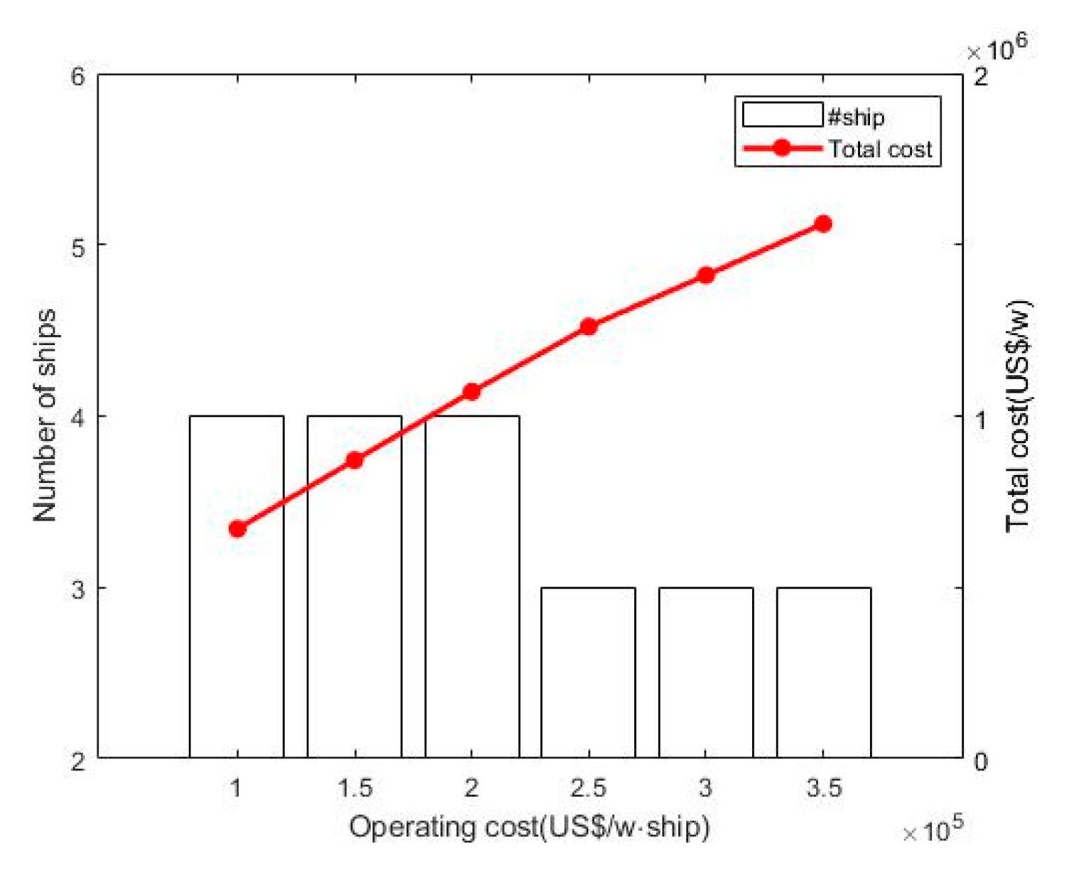
First, we examine the impact of the vessel operating cost on the total cost and the number of ships deployed on the route. We increase the vessel operating cost from US$100,000, US$150,000, US$200,000, US$250,000, and US$300,000 to US$350,000, and the other parameters are the same as those mentioned in Section 4.1. The results are shown in Figure 4 and

Table 2. Optimal arrival time with different operating costs.

Operating Cost (×105 US$)	$\mathbf{Arrival}\mathbf{Time}{\mathit{t}}_{\mathit{i}}^{\mathit{a}}$
	Port 1	Port 2	Port 3	Port 4	Port 5	Port 6	Port 7	Port 8	Port 9	Port 1
1.0	16.06	37.38	97.6	131.03	217.3	337.08	384	418.6	474.22	688.06
1.5	16.06	37.38	97.6	131.03	217.3	337.08	384	418.6	474.22	688.06
2.0	16.06	37.38	97.6	131.03	217.3	337.08	384	418.6	474.22	688.06
2.5	91.05	107.98	152.82	177.47	240	331.94	371.84	400.02	442.97	595.05
3.0	91.05	107.98	152.82	177.47	240	331.94	371.84	400.02	442.97	595.05
3.5	91.05	107.98	152.82	177.47	240	331.94	371.84	400.02	442.97	595.05

. We determine that the number of deployed ships decreases when the vessel operating cost rises to a certain degree, and once the number of deployed ships changes, the optimal arrival time changes; a higher operating cost generally leads to an increase in the total cost of container lines. This indicates that when the vessel operating cost is high, container lines can reduce operating costs by deploying fewer vessels. In general, the total cost increases linearly with the operation cost.

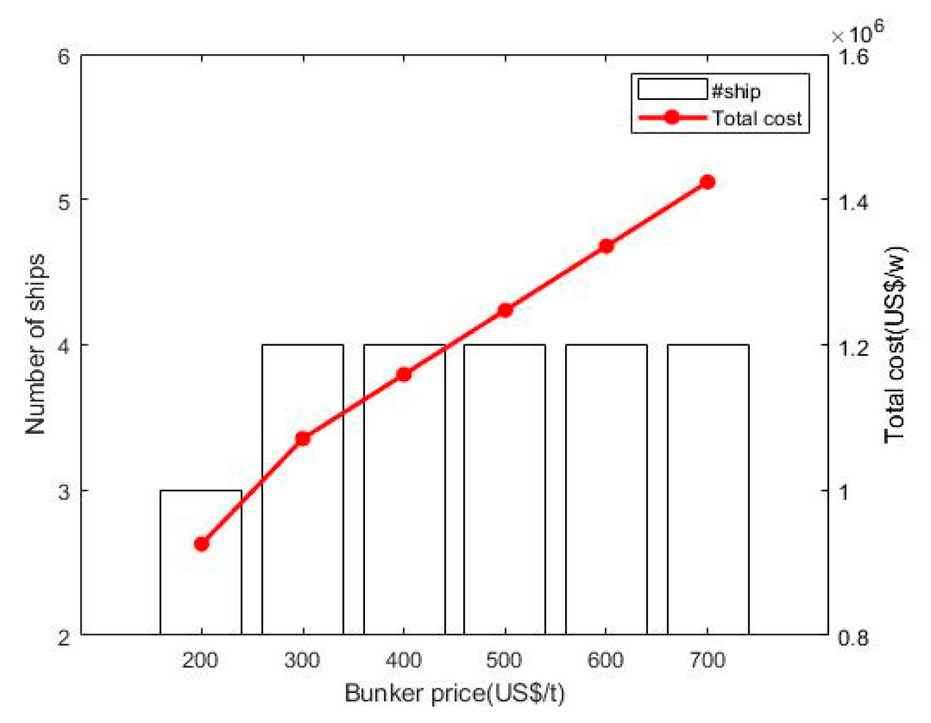
5.3. Effects of Bunker Prices

As the bunker consumption cost is the largest part of the total operating cost, the rise in the bunker price will considerably affect the profit. To study the impact of volatility on bunker price, we set the bunker price from US$200 to US$700, and the other parameters are the same as those mentioned in Section 5.1. Figure 5 shows that a higher bunker price leads to a higher total cost. In terms of the number of ships to be allocated, three ships are deployed only when the bunker cost is as low as US$200, and in the other cases, four ships are deployed.

Table 3. Optimal arrival time with different bunker prices.

Bunker Price (US$/t)	$\mathbf{Arrival}\mathbf{Time}{\mathit{t}}_{\mathit{i}}^{\mathit{a}}$
	Port 1	Port 2	Port 3	Port 4	Port 5	Port 6	Port 7	Port 8	Port 9	Port 1
200	91.05	107.98	152.82	177.47	240	331.94	371.84	400.02	442.97	595.05
300	16.06	37.38	97.6	131.03	217.3	337.08	384	418.6	474.22	688.06
400	15.43	36.76	96.98	130.41	217.3	337.08	384	418.6	474.22	687.43
500	14.7	36.02	96.24	129.67	216.57	337.08	384	418.44	473.93	686.7
600	14.7	36.02	96.24	129.67	216.57	337.08	384	418.44	473.93	686.7
700	14.51	35.83	96.05	129.67	216.57	337.08	384	418.44	473.74	686.51

summarizes that the optimal arrival time varies evidently when the number of vessels varies. These results indicate that the volatility in the bunker price has little impact on the number of ships deployed on the near-sea routes. This is mainly because the length of a round-trip of a near-sea route is always short, and the dwelling time at ports of call takes up a considerable proportion of the total round-trip time. Therefore, there is little room for container lines to adjust the number of ships deployed on the near-sea routes facing fluctuations in bunker prices. Overall, owing to the stability of the number of ships deployed on the near-sea route, the total cost increases linearly with the bunker price.

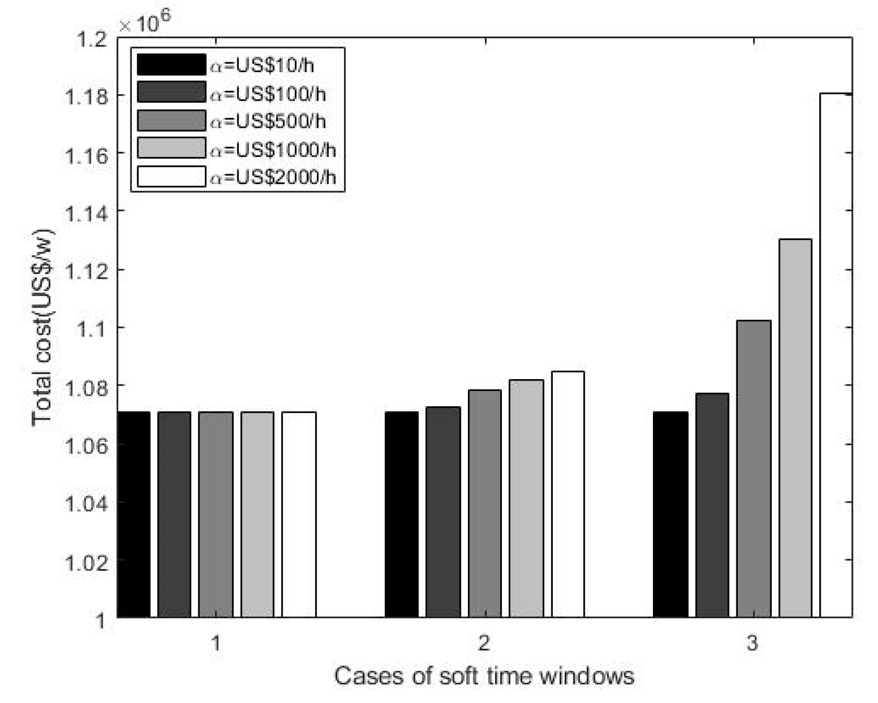
5.4. Comparisons of Port Soft-Time Windows

In this section, we study the impact of the port soft-time windows on the total cost and optimal arrival time. Considering Semarang, Surabaya, and Makassar ports as examples to study the influence of the soft-time window, we set three time-window scenarios, as summarized in

Table 4. Scenarios of soft port times at Semarang, Surabaya, and Makassar.

Port	Scenario of Soft-Time Windows
	1	2	3
Semarang	Monday	Monday	Tuesday
Surabaya	Tuesday	Tuesday	Tuesday
Makassar	Thursday	Wednesday	Tuesday

. Scenario 1 is the default setting. From scenarios 1 to 3, the time windows of the three ports are getting closer. In each scenario, we set the unit penalty cost of the three ports from US$10/h, US$100/h, US$500/h, and US$1000/h to US$2000/h, which indicates that the importance of the big customers is increasing. The results are shown in Figure 6 and

Table 5. Optimal arrival time with different time windows and unit penalty costs.

Scenario	$\mathit{\alpha }$ (US$/h)	$\mathbf{Arrival}\mathbf{Time}{\mathit{t}}_{\mathit{i}}^{\mathit{a}}$
		Port 1	Port 2	Port 3	Port 4	Port 5	Port 6	Port 7	Port 8	Port 9	Port 1
1	10	16.06	37.38	97.6	131.03	217.3	337.08	384	418.6	474.22	688.06
	100	164.77	186.2	246.82	280.25	366.9	486.68	533.78	568.38	624	836.77
	500	164.77	186.2	246.82	280.25	366.9	486.68	533.78	568.38	624	836.77
	1000	164.77	186.2	246.82	280.25	366.9	486.68	533.78	568.38	624	836.77
	2000	164.77	186.2	246.82	280.25	366.9	486.68	533.78	568.38	624	836.77
2	10	62.75	84.08	144.3	177.73	264	383.78	430.88	465.64	521.57	734.75
	100	147.12	168.55	229.17	262.82	350.09	470.6	517.88	552	606.35	819.12
	500	146.36	168.01	229.01	263.12	351.27	472.51	519.97	552	602.55	818.36
	1000	145.7	167.47	228.88	263.21	351.98	474.37	522.19	552.61	600	817.7
	2000	148.38	170.38	232.43	266.98	356.38	479.82	528	556.5	600	820.38
3	10	62.46	83.78	144	177.43	263.7	383.48	430.58	465.34	521.28	734.46
	100	4.96	26.39	87.01	120.44	207.16	326.94	374.04	408	462.67	676.96
	500	3.89	25.55	86.56	120.44	207.96	328.69	375.97	408	458.55	675.89
	1000	2.24	24.02	85.71	119.81	207.96	329.93	377.57	408	455.39	674.24
	2000	1.66	23.66	85.85	120.18	208.95	331.66	379.66	408	451.27	673.66

. In scenario 1, with the increase in the penalty cost, the total cost does not substantially increase. The total cost and optimal arrival time remain the same as the unit penalty cost increases from US$100/h to US$2000/h, which means that when the unit penalty cost is US$100/h, the ship can arrive at the ports within the time windows preferred by the big customers. In scenario 3, the total cost increases with the unit penalty cost. The reason is that the soft-time windows of all three ports are set on the same day, and it is impossible for a container ship to arrive at the three ports on the same day. Therefore, with the increasing unit penalty cost, container lines can only continuously increase the sailing speed on the legs between the three ports to minimize the penalty cost of soft-time windows.

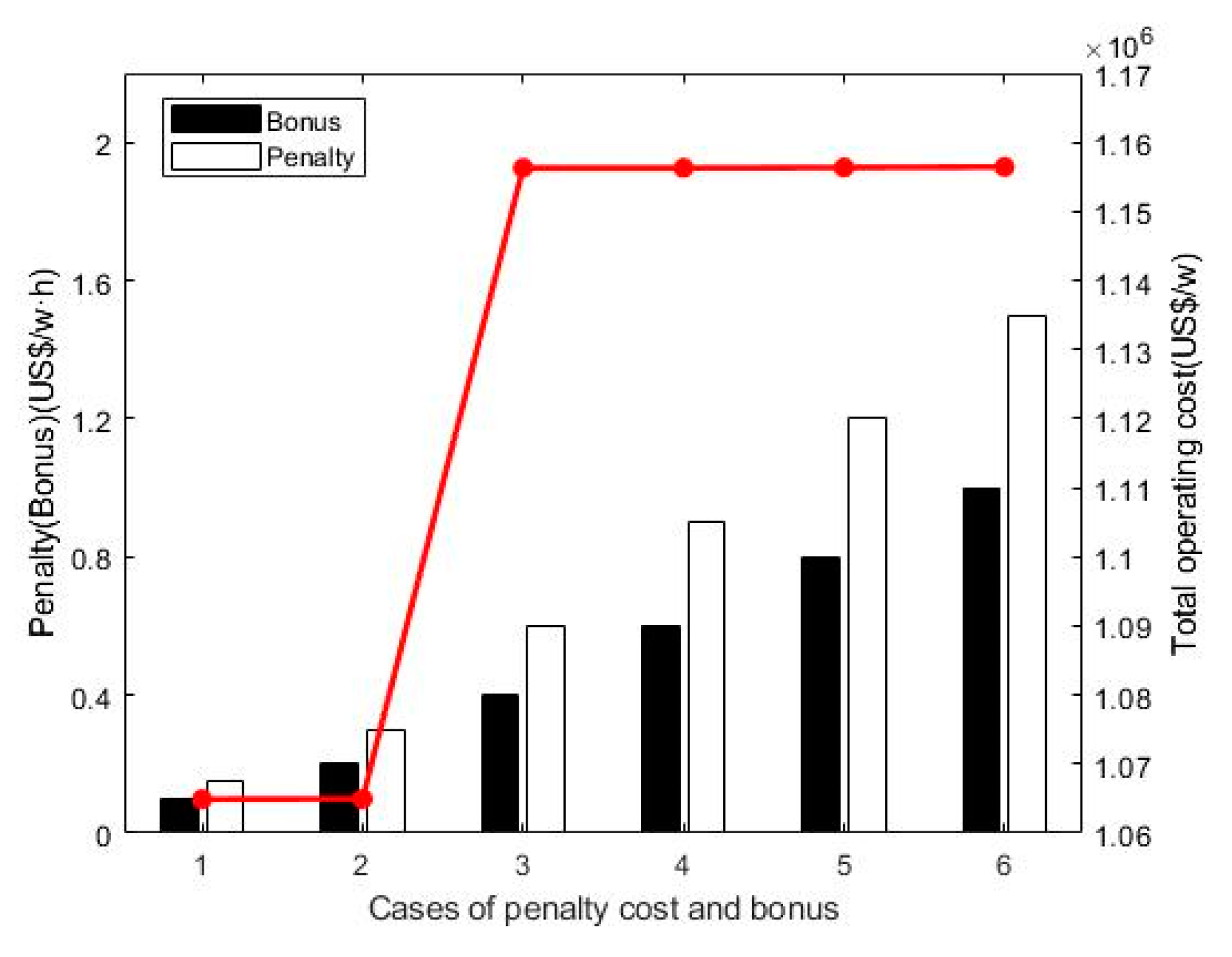
5.5. Effects of Shipping Time Sensitivity

Finally, the sensitivity of the shipping time also affects the total operating cost. We scale up ${\overline{\gamma }}_h$ and ${\tilde{\gamma }}_h$ from US$0.1/h and US$0.15/h to US$1.0/h and US$1.5/h, respectively. The results are shown in Figure 7 and

Table 6. Optimal arrival times with different penalty costs and bonuses.

${\overline{\mathit{\gamma }}}_{\mathit{h}}$ (US$/h)	${\tilde{\mathit{\gamma }}}_{\mathit{h}}$ (US$/h)	Fleet Size	$\mathbf{Arrival}\mathbf{Time}{\mathit{t}}_{\mathit{i}}^{\mathit{a}}$
			Port 1	Port 2	Port 3	Port 4	Port 5	Port 6	Port 7	Port 8	Port 9	Port 1
0.1	0.15	4	15.43	36.76	96.98	130.41	217.3	337.08	384	418.44	473.74	687.43
0.2	0.3	4	16.06	37.38	97.6	131.03	217.3	337.08	384	418.6	474.22	688.06
0.4	0.6	3	91.05	107.98	152.82	177.47	240	331.94	371.84	400.02	442.97	595.05
0.6	0.9	3	96	112.93	157.77	182.42	244.95	336.89	376.79	404.97	447.92	600
0.8	1.2	3	91.67	108.61	153.44	178.09	240	331.94	371.84	400.02	442.97	595.67
1.0	1.5	3	91.67	108.61	153.44	178.09	240	331.21	371.14	399.32	442.27	595.67

; the results demonstrate that when a high proportion of cargoes are time sensitive, that is, when the ship needs to run at a high speed, container lines could reduce the total cost by reducing the number of ships deployed. However, owing to the short voyages of near-sea service routes, container lines have little room to adjust the fleet size.

6. Conclusions and Future Work

This study examines the liner shipping schedule design problem considering the big customers’ preferences for ship arrival time. To this end, we consider the big customers’ preferences for ship arrival times at loading ports, which is of practical significance for maintaining the sustainable development of the liner shipping network, environment, and society. The problem is expressed as a mixed-integer nonconvex nonlinear programming model. The model is then transformed into a mixed-integer linear programming model by reformulating the piecewise functions and approximating the convex nonlinear function through an outer linear approximation technique. The proposed model is solved efficiently by the current mainstream optimization solver to obtain the optimal solution, which proves the applicability of the model to the problem. We conduct a series of numerical experiments by considering CVI, a near-sea route operated by SITC Container Lines, as an example.

The results demonstrate that the big customers’ time preferences affect the total cost, sailing speed on each leg, and ship arrival time. Therefore, considering the big customers’ time preferences is crucial for container lines when designing a ship schedule in practice. In addition, we conducted a sensitivity analysis on the vessel operating cost, bunker price, and shipping time. First, the total cost increases linearly with the operation cost. Second, owing to the short length of a round-trip in near-sea routes, when the bunker price changes, there is little room for container lines to adjust the number of ships deployed on the designed service route. Finally, when the shipping time is urgent, carriers can reduce the total cost by reducing the number of ships deployed, with little room for adjustment.

In future studies, we will extend the problem to a liner shipping network. In addition, it is of great practical significance to study the joint optimization of port call adjustment and ship schedule design with time windows for the adjacent port groups of a certain country on the near-sea routes such as the Kansai port group, the Kanto port group, the Manila north and south ports, and the Laem Chabang and Bangkok ports.

References

- UNCTAD. Review of Maritime Transport 2019. In Paper Presented at the United Nations Conference on Trade and Development, New York and Geneva. Available online: https://unctad.org/en/PublicationsLibrary/rmt2019_en.pdf (accessed on 31 January 2020).
- Zis, T.P.V.; Cullinane, K. The desulphurisation of shipping: Past, present and the future under a global cap. Transp. Res. Part D Transp. Environ. 2020, 82, 102316. [Google Scholar] [CrossRef]
- Zis, T.; Psaraftis, H.N. The implications of the new sulphur limits on the European Ro-Ro sector. Transp. Res. Part D Transp. Environ. 2017, 52, 185–201. [Google Scholar] [CrossRef] [Green Version]
- Fagerholt, K. Ship scheduling with soft time windows: An optimisation based approach. Eur. J. Oper. Res. 2001, 131, 559–571. [Google Scholar] [CrossRef]
- Corbett, J.J.; Wang, H.; Winebrake, J.J. The effectiveness and costs of speed reductions on emissions from international shipping. Transp. Res. Part D Transp. Environ. 2009, 14, 593–598. [Google Scholar] [CrossRef]
- Psaraftis, H.N.; Kontovas, C.A. Speed models for energy-efficient maritime transportation: A taxonomy and survey. Transp. Res. Part C Emerg. Technol. 2013, 26, 331–351. [Google Scholar] [CrossRef]
- Lindstad, H.; Asbjornslett, B.E.; Stromman, A.H. Reductions in greenhouse gas emissions and cost by shipping at lower speeds. Energy Policy 2011, 39, 3456–3464. [Google Scholar] [CrossRef]
- Wang, S.; Meng, Q. Schedule design and container routing in liner shipping. Transp. Res. Rec. J. Transp. Res. Board 2011, 2222, 25–33. [Google Scholar] [CrossRef]
- Christiansen, M.; Fagerholt, K.; Nygreen, B.; Ronen, D. Ship routing and scheduling in the new millennium. Eur. J. Oper. Res. 2013, 228, 467–483. [Google Scholar] [CrossRef]
- Meng, Q.; Wang, S.; Andersson, H.; Thun, K. Containership routing and scheduling in liner shipping: Overview and future research directions. Transp. Sci. 2014, 48, 265–280. [Google Scholar] [CrossRef] [Green Version]
- Tran, N.K.; Haasis, H. Literature survey of network optimization in container liner shipping. Flex. Serv. Manuf. J. 2015, 27, 139–179. [Google Scholar] [CrossRef]
- Wang, S.; Meng, Q. Container liner fleet deployment: A systematic overview. Transp. Res. Part C Emerg. Technol. 2017, 77, 389–404. [Google Scholar] [CrossRef]
- Lee, C.; Song, D. Ocean container transport in global supply chains: Overview and research opportunities. Transp. Res. Part B Methodol. 2017, 95, 442–474. [Google Scholar] [CrossRef]
- Agarwal, R.; Ergun, O. Ship scheduling and network design for cargo routing in liner shipping. Transp. Sci. 2008, 42, 175–196. [Google Scholar] [CrossRef]
- Shintani, K.; Imai, A.; Nishimura, E.; Papadimitriou, S. The container shipping network design problem with empty container repositioning. Transp. Res. Part E Logist. Transp. Rev. 2007, 43, 39–59. [Google Scholar] [CrossRef] [Green Version]
- Wang, S.; Meng, Q. Liner shipping network design with deadlines. Comput. Oper. Res. 2014, 41, 140–149. [Google Scholar] [CrossRef]
- Wang, Y.; Meng, Q.; Kuang, H. Intercontinental liner shipping service design. Transp. Sci. 2019, 53, 344–364. [Google Scholar] [CrossRef]
- Kim, H.; Son, D.; Yang, W.; Kim, J. Liner ship routing with speed and fleet size optimization. KSCE J. Civ. Eng. 2019, 23, 1341–1350. [Google Scholar] [CrossRef]
- Koza, D.F.; Desaulniers, G.; Ropke, S. Integrated liner shipping network design and scheduling. Transp. Sci. 2020, 54, 512–533. [Google Scholar] [CrossRef] [Green Version]
- Qi, X.; Song, D. Minimizing fuel emissions by optimizing vessel schedules in liner shipping with uncertain port times. Transp. Res. Part E Logist. Transp. Rev. 2012, 48, 863–880. [Google Scholar] [CrossRef]
- Song, D.; Li, D.; Drake, P. Multi-objective optimization for planning liner shipping service with uncertain port times. Transp. Res. Part E Logist. Transp. Rev. 2015, 84, 1–22. [Google Scholar] [CrossRef]
- Notteboom, T.E.; Vernimmen, B. The effect of high fuel costs on liner service configuration in container shipping. J. Transp. Geogr. 2009, 17, 325–337. [Google Scholar] [CrossRef]
- Ronen, D. The effect of oil price on containership speed and fleet size. J. Oper. Res. Soc. 2017, 62, 211–216. [Google Scholar] [CrossRef]
- Cheaitou, A.; Cariou, P. Liner shipping service optimisation with reefer containers capacity: An application to northern Europe-South America trade. Marit. Policy Manag. 2012, 39, 589–602. [Google Scholar] [CrossRef]
- Meng, Q.; Wang, S. Optimal operating strategy for a long-haul liner service route. Eur. J. Oper. Res. 2011, 215, 105–114. [Google Scholar] [CrossRef]
- Wang, S.A.; Meng, Q. Liner ship fleet deployment with container transshipment operations. Transp. Res. Part E Logist. Transp. Rev. 2012, 48, 470–484. [Google Scholar] [CrossRef]
- Wang, S.; Meng, Q. Sailing speed optimization for container ships in a liner shipping network. Transp. Res. Part E Logist. Transp. Rev. 2012, 48, 701–714. [Google Scholar] [CrossRef]
- Kontovas, C.; Psaraftis, H.N. Reduction of emissions along the maritime intermodal container chain: Operational models and policies. Marit. Policy Manag. 2011, 38, 451–469. [Google Scholar] [CrossRef]
- Xia, J.; Li, K.X.; Ma, H.; Xu, Z. Joint planning of fleet deployment, speed optimization, and cargo allocation for liner shipping. Transp. Sci. 2015, 49, 922–938. [Google Scholar] [CrossRef]
- Du, G.; Sun, C.; Weng, J. Liner shipping fleet deployment with sustainable collaborative transportation. Sustainability 2016, 8, 165. [Google Scholar] [CrossRef] [Green Version]
- Zhen, L.; Wang, S.; Laporte, G.; Hu, Y. Integrated planning of ship deployment, service schedule and container routing. Comput. Oper. Res. 2019, 104, 304–318. [Google Scholar] [CrossRef]
- Sheng, D.; Meng, Q.; Li, Z. Optimal vessel speed and fleet size for industrial shipping services under the emission control area regulation. Transp. Res. Part C Emerg. Technol. 2019, 105, 37–53. [Google Scholar] [CrossRef]
- Fan, H.; Yu, J.; Liu, X. Tramp ship routing and scheduling with speed optimization considering carbon emissions. Sustainability 2019, 11, 6367. [Google Scholar] [CrossRef] [Green Version]
- Yang, L.; Chen, G.; Zhao, J.; Rytter, N.G.M. Ship speed optimization considering ocean currents to enhance environmental sustainability in maritime shipping. Sustainability 2020, 12, 3649. [Google Scholar] [CrossRef]
- Psaraftis, H. Speed optimization vs. speed reduction: The choice between speed limits and a bunker levy. Sustainability 2019, 11, 2249. [Google Scholar] [CrossRef] [Green Version]
- Giovannini, M.; Psaraftis, H.N. The profit maximizing liner shipping problem with flexible frequencies: Logistical and environmental considerations. Flex. Serv. Manuf. J. 2018, 31, 567–597. [Google Scholar] [CrossRef] [Green Version]
- Fagerholt, K.; Johnsen, T.A.V.; Lindstad, H. Fleet deployment in liner shipping: A case study. Marit. Policy Manag. 2009, 36, 397–409. [Google Scholar] [CrossRef]
- Andersson, H.; Fagerholt, K.; Hobbesland, K. Integrated maritime fleet deployment and speed optimization: Case study from RoRo shipping. Comput. Oper. Res. 2015, 55, 233–240. [Google Scholar] [CrossRef]
- Patricksson, O.S.; Fagerholt, K.; Rakke, J.G. The fleet renewal problem with regional emission limitations: Case study from Roll-on/Roll-off shipping. Transp. Res. Part C Emerg. Technol. 2015, 56, 346–358. [Google Scholar] [CrossRef]
- Fischer, A.; Nokhart, H.; Olsen, H.; Fagerholt, K.; Rakke, J.G.; Stalhane, M. Robust planning and disruption management in roll-on roll-off liner shipping. Transp. Res. Part E Logist. Transp. Rev. 2016, 91, 51–67. [Google Scholar] [CrossRef] [Green Version]
- Christiansen, M.; Fagerholt, K. Robust ship scheduling with multiple time windows. Nav. Res. Logist. 2002, 49, 611–625. [Google Scholar] [CrossRef]
- De, A.; Mamanduru, V.K.R.; Gunasekaran, A.; Subramanian, N.; Tiwari, M.K. Composite particle algorithm for sustainable integrated dynamic ship routing and scheduling optimization. Comput. Ind. Eng. 2016, 96, 201–215. [Google Scholar] [CrossRef]
- Kim, J.; Kim, H.; Jun, H.B.; Kim, C. Optimizing ship speed to minimize total fuel consumption with multiple time windows. Math. Probl. Eng. 2016, 2016, 1–7. [Google Scholar] [CrossRef]
- Aydin, N.; Lee, H.; Mansouri, S.A. Speed optimization and bunkering in liner shipping in the presence of uncertain service times and time windows at ports. Eur. J. Oper. Res. 2017, 259, 143–154. [Google Scholar] [CrossRef] [Green Version]
- Hvattum, L.M.; Norstad, I.; Fagerholt, K.; Laporte, G. Analysis of an exact algorithm for the vessel speed optimization problem. Networks 2013, 62, 132–135. [Google Scholar] [CrossRef]
- Wang, S.; Alharbi, A.; Davy, P. Ship route schedule based interactions between container shipping lines and port operators. In Handbook of Ocean Container Transport Logistics: Making Global Supply Chains Effective; Lee, C., Meng, Q., Eds.; Springer International Publishing: Cham, Switzerland, 2015; pp. 279–313. [Google Scholar]
- Wang, S.; Alharbi, A.; Davy, P. Liner ship route schedule design with port time windows. Transp. Res. Part C Emerg. Technol. 2014, 41, 1–17. [Google Scholar] [CrossRef] [Green Version]
- Alharbi, A.; Wang, S.; Davy, P. Schedule design for sustainable container supply chain networks with port time windows. Adv. Eng. Inform. 2015, 29, 322–331. [Google Scholar] [CrossRef]
- Dulebenets, M.A. The vessel scheduling problem in a liner shipping route with heterogeneous fleet. Int. J. Civ. Eng. 2018, 16, 19–32. [Google Scholar] [CrossRef]
- Yu, B.; Peng, Z.; Tian, Z.; Yao, B. Sailing speed optimization for tramp ships with fuzzy time window. Flex Serv. Manuf. J. 2019, 31, 308–330. [Google Scholar] [CrossRef]
- Zis, T.; North, R.J.; Angeloudis, P.; Ochieng, W.Y.; Harrison Bell, M.G. Evaluation of cold ironing and speed reduction policies to reduce ship emissions near and at ports. Marit. Econ. Logist. 2014, 16, 371–398. [Google Scholar] [CrossRef]
Figure 1.
CVI service provided by SITC (2018).
Figure 2.
(a) Penalty function image of soft-time windows for Wednesday; (b) penalty function image of soft-time windows for Friday.
Figure 3.
Penalty function image of soft-time windows for each day of the week.
Figure 4.
Impact of operating costs.
Figure 5.
Impact of bunker prices.
Figure 6.
Impact of soft-time windows.
Figure 7.
Impact of the sensitivity of shipping time.