Development of the CREATE Inventory in Support of Integrated Climate and Air Quality Modeling for Asia

Abstract

A bottom-up emissions inventory is one of the most important data sets needed to understand air quality (AQ) and climate change (CC). Several emission inventories have been developed for Asia, including Transport and Chemical Evolution over the Pacific (TRACE-P), Regional Emission Inventory in Asia (REAS), and Inter-Continental Chemical Transport Experiment (INTEX) and, while these have been used successfully for many international studies, they have limitations including restricted amounts of information on pollutant types and low levels of transparency with respect to the polluting sectors or fuel types involved. To address these shortcomings, we developed: (1) a base-year, bottom-up anthropogenic emissions inventory for Asia, using the most current parameters and international frameworks (i.e., the Greenhouse gas—Air pollution INteractions and Synergies (GAINS) model); and (2) a base-year, natural emissions inventory for biogenic and biomass burning. For (1), we focused mainly on China, South Korea, and Japan; however, we also covered emission inventories for other regions in Asia using data covering recent energy/industry statistics, emission factors, and control technology penetration. The emissions inventory (Comprehensive Regional Emissions inventory for Atmospheric Transport Experiment (CREATE)) covers 54 fuel classes, 201 subsectors, and 13 pollutants, namely SO₂, NO_x, CO, non-methane volatile organic compounds (NMVOC), NH₃, OC, BC, PM₁₀, PM_2.5, CO₂, CH₄, N₂O, and Hg. For the base-year natural emissions inventory, the Model of Emissions of Gases and Aerosols from Nature (MEGAN) and BlueSky-Asia frameworks were used to estimate biogenic and biomass burning emissions, respectively. Since the CREATE emission inventory was designed/developed using international climate change/air quality (CC/AQ) assessment frameworks, such as GAINS, and has been fully connected with the most comprehensive emissions modeling systems—such as the US Environmental Protection Agency (EPA) Chemical Manufacturing Area Source (CMAS) system—it can be used to support various climate and AQ integrated modeling studies, both now and in the future.

1. Introduction

In recent decades, Asia has become increasingly populous, and its economies have grown rapidly, to the extent that East Asia has become the largest emission region in the world due to this large population and the increased energy use caused by its economic growth. From the perspective of the global atmospheric environment, Asia is a critical source of air pollution, and this has become a more serious issue here than in other regions—and lately has begun to receive international attention [1,2,3].

This problem can be resolved through long-term joint efforts and adoption of best practices, and this approach needs to be supported by objective and scientific data. Systematic tracking of air pollution sources and emissions data organization forms the most effective basis for understanding air pollution processes and deriving policy solutions. This includes collating pollutant emissions by region, sector, and fuel-type, within a comprehensive anthropogenic emissions inventory.

Several emissions inventories have been developed covering Asia; these include TRACE-P (Transport and Chemical Evolution over the Pacific) [4], INTEX-B (Intercontinental Chemical Transport Experiment-Phase B) [5], REAS (Regional Emission inventory in Asia) [2], and EDGAR (Emission Database for Global Atmospheric Research) [6]. Two methods have been used to develop these emissions inventories; the first method uses fundamental data, such as energy use activities, emission factors, and controlling policies, and the second method assembles a mosaic of emissions inventories from different countries or regions. The first method is more structural and informative, as it includes most of the information necessary to understand the socioeconomic, technological, and policy background applicable over the domain—although it has the drawback that limited data are available for some countries and regions. The second method is advantageous because it provides better total emissions estimates for developed countries/regions; however, it can be limited by the amount of fundamental information needed to estimate emissions.

As Asian countries are at various developmental stages, inventory methodologies must be equipped to reflect their rapid socioeconomic changes and policy initiatives. If this can be achieved, while it may not lead to the most accurate emissions estimates, it can represent a system that explains the current situation, predict likely future emissions scenarios, and can be applied to air quality (AQ) studies. Fundamentally, building an integrated emissions modeling inventory can improve both air pollution predictability and climate change (CC) modeling accuracy.

Biogenic emissions play an important role in regional AQ and global atmospheric chemistry. Open biomass burning emissions are a major source of air pollution and can influence global CC through both greenhouse gases (GHGs) and aerosols emissions and vegetation cover losses. Information on natural emission sources is generally quite poor because most emission inventory studies have primarily targeted anthropogenic emissions.

In response to these issues, we developed the Comprehensive Regional Emissions Inventory for Atmospheric Transport Experiment (CREATE) to cover Asian emissions and to support scientific studies and policy development in the region. The CREATE inventory was developed using activities, emission factors, and controls, as these were helpful in estimating not only base year emissions but also present and future year emission scenarios. Our objective was to design and develop an inventory scheme that provides better support for AQ modeling and which can be operated in concert with the Sparse Matrix Operator Kernel Emissions for Asia (SMOKE-Asia) emissions processing system [7]. CREATE includes anthropogenic, biogenic, and biomass burning emissions.

2. Methodology and Key Parameters

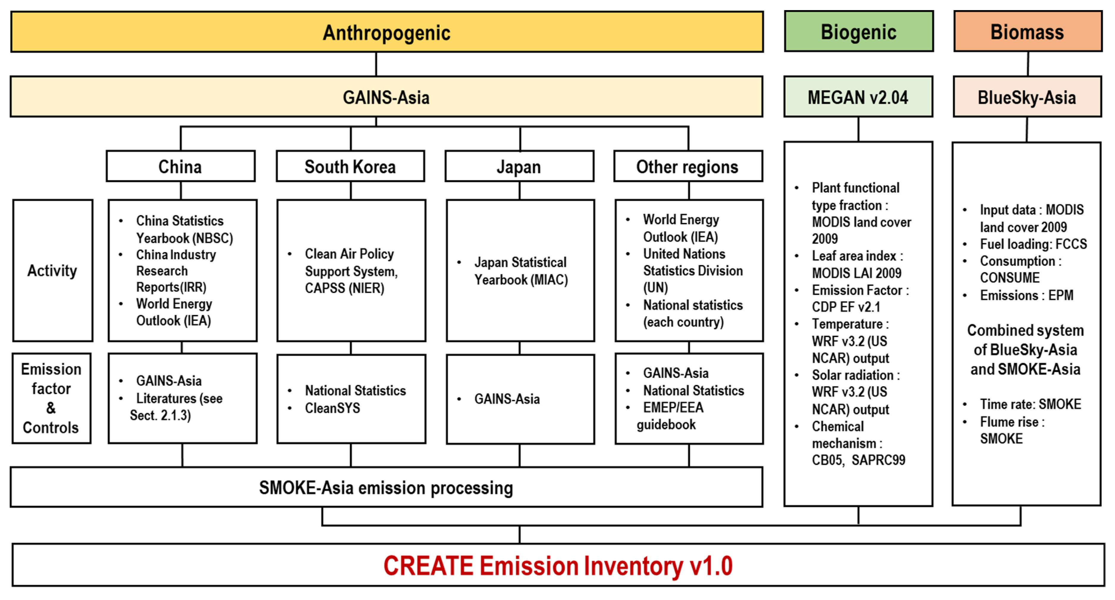
2.1. Anthropogenic Emissions

2.1.1. GAINS Framework

Our emissions calculations were developed using the Greenhouse Gas and Air Pollution Interactions and Synergies-Asia (GAINS-Asia) model (http://gains.iiasa.ac.at). GAINS was launched in 2006 as an extension to the Regional Air Pollution and Simulation (RAINS) model, which had been used to assess cost-effective response strategies for combating air pollution elements such as fine particulates and ground-level ozone. GAINS provides an authoritative framework for assessing strategies for reducing multiple air pollutant GHG emissions, with the objective of minimizing their negative effects on human health, ecosystems, and climate change (CC), using a least-cost approach.

For each pollutant, GAINS can be applied to estimate emissions based on activity data, uncontrolled emission factors, and emission control measure removal efficiencies, as well as the extent to which such measures have been implemented. For a given country, i, and pollutant, p, considered in a study, this is achieved using Equation (1) [8]:

$$E_{i,p}={\displaystyle \sum }_k{\displaystyle \sum }_m{A}_{i,k}·e{f}_{i,k,m,p}·x_{i,k,m,p}$$

(1)

where, i, k, m, and p represent the region, activity type, abatement measure, and pollutant, respectively. E_p stands for the emission of pollutant p, A_i,k represents activity data of type k in region i, ef_I,k,m,p stands for the emission factor for pollutant p in region i for activity k, after application of control measure m (where m includes the “no control” situation), and x_I,k,m,p stands for penetration of region i by control measure m for pollutant p from activity k.

This approach incorporates emissions reduction calculation by changing each input parameter and/or making minor structural changes to ensure that the GAINS framework emissions data simplifies evaluation of emission changes as a result of socioeconomic and/or environmental policies.

2.1.2. Activity Data

Input parameter formats and methodologies generally differ from country to country. For our modeling, activity data were obtained mostly from World Energy Balance statistics produced by the International Energy Agency (IEA) [9], while in some cases (China, S. Korea, N. Korea, and Japan), official national data were used.

Activity data incorporated into the CREATE inventory, included IEA statistics for the whole of the research domain, the 2010 Energy Statistical Yearbook for China (CESY 2010) [10], the Clean Air Policy Support System (CAPSS) [11] for S. Korea, the Japan Statistical Yearbook (JSY) [12], and several domestic documents released by S. Korea for N. Korea. United Nations (UN) Energy Statistics Database (UN, 2011) [13] energy balance data were used for some countries not covered by IEA data, and non-energy activity data were collected from various international, national, and regional statistics sources, from previous studies, and from official UN Statistics Division documents.

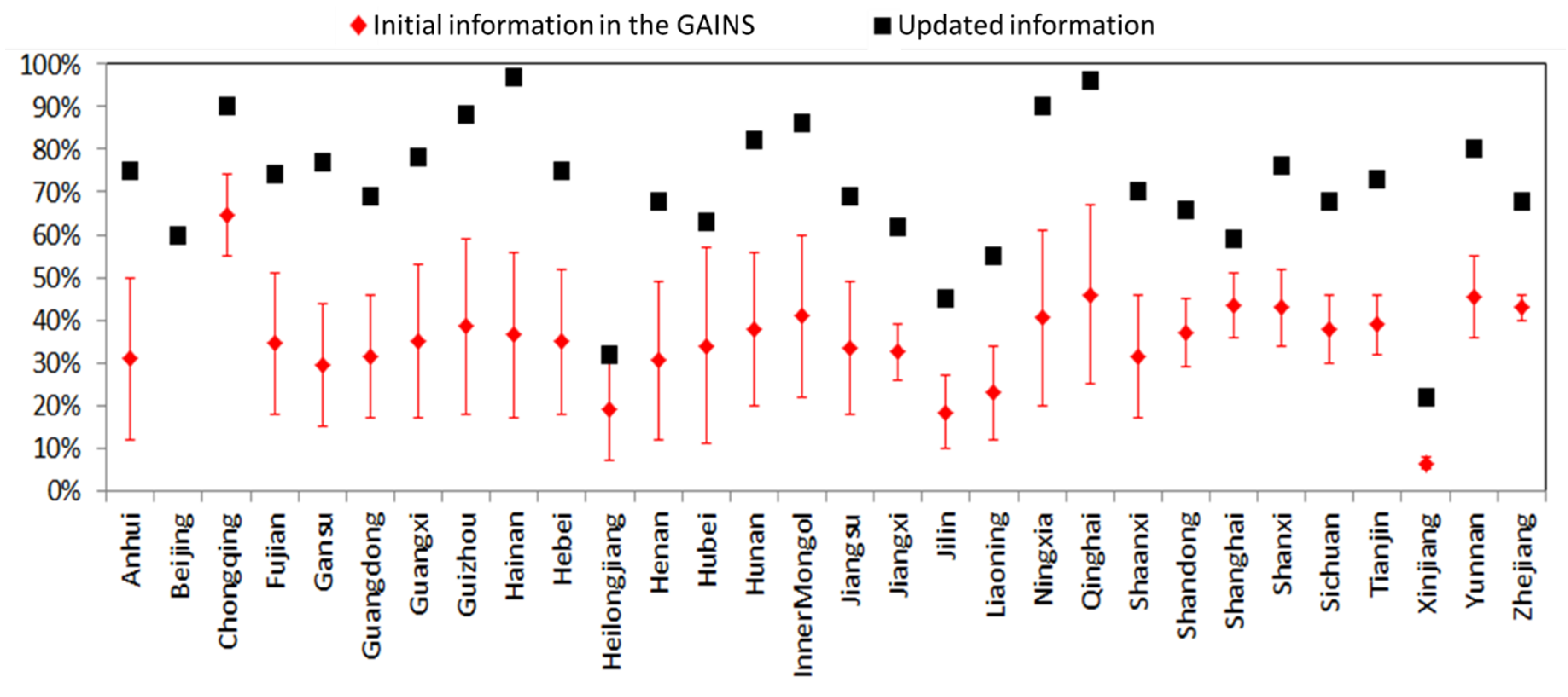
2.1.3. Emission Factors and Control Technologies

We used GAINS-Asia emission factors and removal efficiencies as default data where local information was absent, and updated CREATE by including recent regional/national control policies that could be sourced from the literature. For S. Korea, we achieved these updates using activity, emissions, and removal factors published in the CAPSS 2010 official emissions inventory. We viewed the quality of N. Korean emission input-related data as being rather uncertain due to the difficulty in accessing relevant information, and so derived N. Korea input parameters by extrapolating gross domestic product (GDP), population, and industrial activity indexes from S. Korea into N. Korea.

China is the biggest regional energy consumer; however, it has aggressively applied various environmental protection policies. To capture their effects, we reviewed relevant literature (B. Zhao et al., 2013 [14]; Zhang et al., 2009 [5]; Hong et al., 2012 [15]; Y. Zhao et al., 2010 [16]; Lei et al., 2011 [17]; Y. Zhao et al., 2012 [18]) to update the characterization of input parameters, such as removal efficiencies and control technology penetration rates, in the GAINS model [19]. As an example, the initial input parameters in GAINS-Asia and updated flue gas desulfurization (FGD) technology penetration information have been presented in Figure 1, where the revised information shows that most Chinese provinces have achieved high improvement implementation rates.

2.2. Natural Emissions

2.2.1. Biogenic Emissions: The MEGAN Model

Biogenic volatile organic compounds (BVOCs) emitted by plants are important in emission and air pollution research, as they are significant contributors of secondary air pollutants, including ozone and secondary fine particles [20,21,22].

Previous studies on global BVOC emissions (e.g., Guenther et al., 1995; Intergovermental Panel on Climate Change (IPCC), 2007 [23,24]) have reported that they exceed anthropogenic source emissions. Among BVOCs, isoprene (C₅H₈) has been noted as the dominant chemical compound, accounting for up to 50% of total BVOCs [23]. BVOCs affect the formation of secondary organic aerosols (SOAs) and tropospheric ozone, as well as radiative forcing, which can influence not only the air quality but also the climate [25,26,27]. This implies that accurately estimating BVOC atmospheric emissions is important if their role in chemical transport models and their climatic impacts are to be accurately represented. BVOC emissions are often not listed in emissions inventories or have been simply estimated when needed as inputs into AQ modeling studies.

In this study, we used the Model of Emissions of Gases and Aerosols from Nature (MEGAN) v2.04 to estimate BVOC emissions and develop BVOC emissions inventories for Asia. MEGAN is a modeling framework for estimating temporal and spatial emission rates of chemical compounds from the vegetation in the terrestrial ecosystems to the atmosphere [28,29]. In general, the equation for calculating natural vegetation emission is as shown in Equation (2):

$$F_i={\gamma }_i\sum {\epsilon }_{i,j}{\chi }_j$$

(2)

where F_i represents emissions of chemical species i (as μg/m²h⁻¹), ${\gamma }_i$ denotes emission activity for chemical species i, ε_i,j represents the standard emission factor for chemical species i from vegetation type j, and χ_j indicates the percentage of vegetation type j occupying a grid square [28].

We prepared vegetation input variables (basically plant functional type (PFT), leaf area index (LAI)), emission factors (EFs), and main metrological variables (TEMP., for temperature, and RAD., for solar radiation)) related to vegetation emissions as input data for calculating BVOC emissions with MEGAN. Meteorological data were estimated using the Weather Research and Forecasting (WRF) model, and EFs were derived using the database of the MEGAN development group released through the community data portal (http://cdp.ucar.edu) maintained by the US National Center for Atmospheric Research (NCAR). PFT and LAI database used in this study were developed by using the Moderate Resolution Imaging Spectroradiometer (MODIS) land cover (LC) and leaf area index (LAI) product of the Terra and Aqua satellite sensors, which were recategorized and converted for inputting into MEGAN. Details on the preparation of vegetation input variables (i.e., PFT and LAI) utilizing MODIS LC and LAI products are documented in Kim et al. [30]. Through the implementation of MEGAN using these input variables, we developed gridded BVOC emissions data, and then generated a country-based, annual BVOCs emissions inventory for Asia.

We tried to maintain speciated emissions by two different types of chemical mechanisms (i.e., CB05 and SAPRC99 [31,32]) in order to open a possibility to support multiple possible simulation setups in Chemical Transport Models (CTMs) (

Table 1. Modeling Parameters Information.

Parameters	Source	Description
MEGAN model	2.04 (US NCAR)	Guenther et al. (2006) [28]
Chemical Mechanism	CB05 (1) and SAPRC99 (2)	Yarwood et al. (2005) [31], Carter, W.P.L. (2000) [32]
Temperature data	WRF v3.2 (US NCAR)	TEMP2(K) (3)
Solar radiation data	WRF v3.2 (US NCAR)	RGRND(W/m2) (4)
PFTF	MODIS land cover 2009	https://wist.echo.nasa.gov/api/
LAI	MODIS LAI 2009	https://wist.echo.nasa.gov/api/
Emission factor data source	MEGAN EFv2.1	http://cdp.ucar.edu

⁽¹⁾ Carbon Bond (CB05) mechanism, ⁽²⁾ State Air Pollution Research Center 99, ⁽³⁾ Air temperature at 2 m above ground, ⁽⁴⁾ Solar radiation absorbed at ground.

).

In this study, the simulation with the WRF version 3.2 was conducted on a domain using 60 km × 60 km horizontal resolution with 148 × 184 cells in the horizontal direction and 32 layers in the vertical direction. The 6 hourly NCEP (National Centers for Environmental Prediction) data with 1° × 1° grid resolution were used for the initial meteorological condition for the WRF simulation. The simulation was conducted over one year. More detailed configuration of WRF is described in

Table 2. Configuration of the Weather Research and Forecasting (WRF) model simulation [33].

Item	Description
WRF version	WRFv3.2
Resolution	60 km × 60 km
Horizontal Number of Grids	148 × 184
Number of Vertical layers	32 layers
Initial Conditions	1° × 1° and every six hours data from the National Centers for Environmental Prediction Final (NCEP FNL) (http://dss.ucar.edu/datasets/ds083.2/)
Topography Data	30 s USGS
Microphysics	WSM6 (1) (WRF Single-Moment 6-Class)
longwave radiation	RRTM (Rapid Radiative Transfer Model) scheme
shortwave radiation	Dudhia scheme
surface-layer options	Monin-Obukhov scheme
PBL physics	YSU (2) scheme
Cumulus physics	Kain-Fritsch (new Eta) scheme
Surface physics	Unified Noah land-surface model

⁽¹⁾ Weather Research and Forecasting Single Moment 6, ⁽²⁾ YonSei University.

.

2.2.2. Biomass Burning Emissions: The BlueSky-Asia Model

The biomass burning estimation method used in this study was based on the BlueSky model developed by the US Department of Agriculture Forest Service and the US EPA. It was designed to facilitate the production of predictive models for calculating cumulative impacts from smoke on AQ, and from forest, agricultural, and range fire emissions [34,35]. In this study, we decided to use Fuel Characteristic Classification System (FCCS) data for three fuel loadings mapped in BlueSky, as they provided a more detailed fuel classification structure compared with other database options. Total fuel consumption was estimated using the CONSUME model (which outputs fuel consumption and emissions by combustion phase), and emissions were calculated based on the BlueSky emissions production model. The domain for our biomass emissions inventory covered not only Asia, but also Siberia and parts of central Asia, as these regions have histories of large-scale fires that can affect our target region.

To generate fire and fuel loading information, we used the MCD45A1 MODIS product [36], which provides fire data (Burned-area Product (BAP)) for fuel-loading calculations, as well as land cover information for biomass classification. BAP information is delivered with a relatively high (daily) temporal resolution and medium-scale (500 m grid) spatial resolution; each fire event is represented by one polygon, which contains the number of burned-area pixels detected (total area burned), date of burning, and location. Such polygons were used as inputs for fire event plume-rise calculations and for biomass-burning emission calculations.

We created a new fuel map (using the MODIS land cover data) for the fuel loading process [37,38], and daily emission estimates from each fire were calculated using this process. Emissions from biomass burning were then estimated for 2008 using the developed modeling framework. We linked this output to the SMOKE processing system to generate input emission data for a three-dimensional, chemical transport model. By combining these two tools, open biomass fires could be modeled, and fire emission AQ impact simulations could be improved. The methodology and results associated with the biomass burning part of the CREATE inventory were described in more detail in Choi et al. 2013 [35].

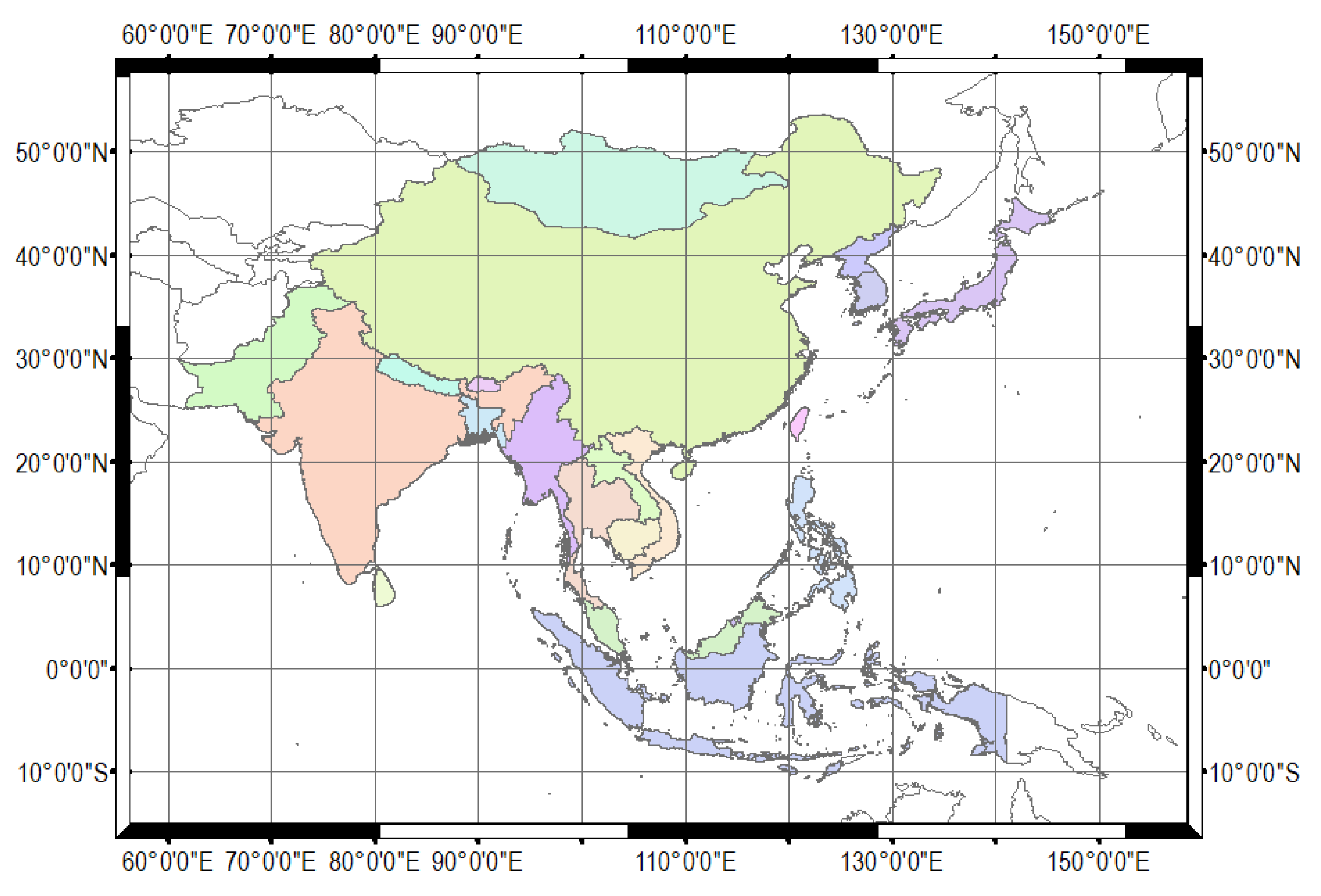
2.3. Research Framework and Domain Setting

The overall framework for biomass-burning, anthropogenic, and biogenic emissions estimation is presented in Figure 2.

Domain, species, and data source information is presented in

Table 3. Contents and scope of CREATE inventory.

Item	Description
Domain	22 countries and 99 regions
Countries and region	Bangladesh(two regions), Bhutan, Brunei Darussalam, Cambodia, China (32 regions), India (23 regions), Indonesia (four regions), Japan (six regions), Democratic People’s Republic of Korea, Republic of Korea (four regions), Laos, Malaysia (three regions), Mongolia, Myanmar, Nepal, Pakistan (four regions), Philippines (three regions), Singapore, Sri Lanka, Taiwan, Thailand (five regions), Vietnam (two regions)
Species	CO, NOx, SO2, Primary PM10 and PM2.5, VOCs, NH3, CO2, CH4, N2O
Sector	Powerplant, Industry, Residential, Transportation, Other (54 fuel classes, 201 Sub-sectors)
Source	Anthropogenic, Biogenic, Biomass burning
Year Data Access	2010 http://aisl.konkuk.ac.kr/#/emission_data/create_emission_inventory

. Emissions for 22 countries (99 regions) were compiled in the CREATE inventory, covering the geographical domain shown in Figure 3.

The main pollutant sources and categories in the CREATE emissions inventory are explained in

Table 4. Classification of emissions by source.

Sector		SO2	NOx	CO	* PM10	* PM2.5	NMVOC	CO2	N2O	NH3	CH4
Anthropogenic	Combustion/Non-combustion/ Agriculture, etc.	●	●	●	●	●	●	●	●	●	●
Natural	Biomass Burning		●	●		●	●
	Biogenic		●	●			●		●	●	●

* Primary PM₁₀ and PM_2.5.

. The methodologies and parameters explained in Section 2 were used to estimate emissions for CREATE, and in Section 3, emission estimation results have been discussed as follows: (1) anthropogenic emissions in 2010; (2) natural source emissions; (3) comparisons with other studies; (4) analysis of uncertainty.

3. Results and Discussion

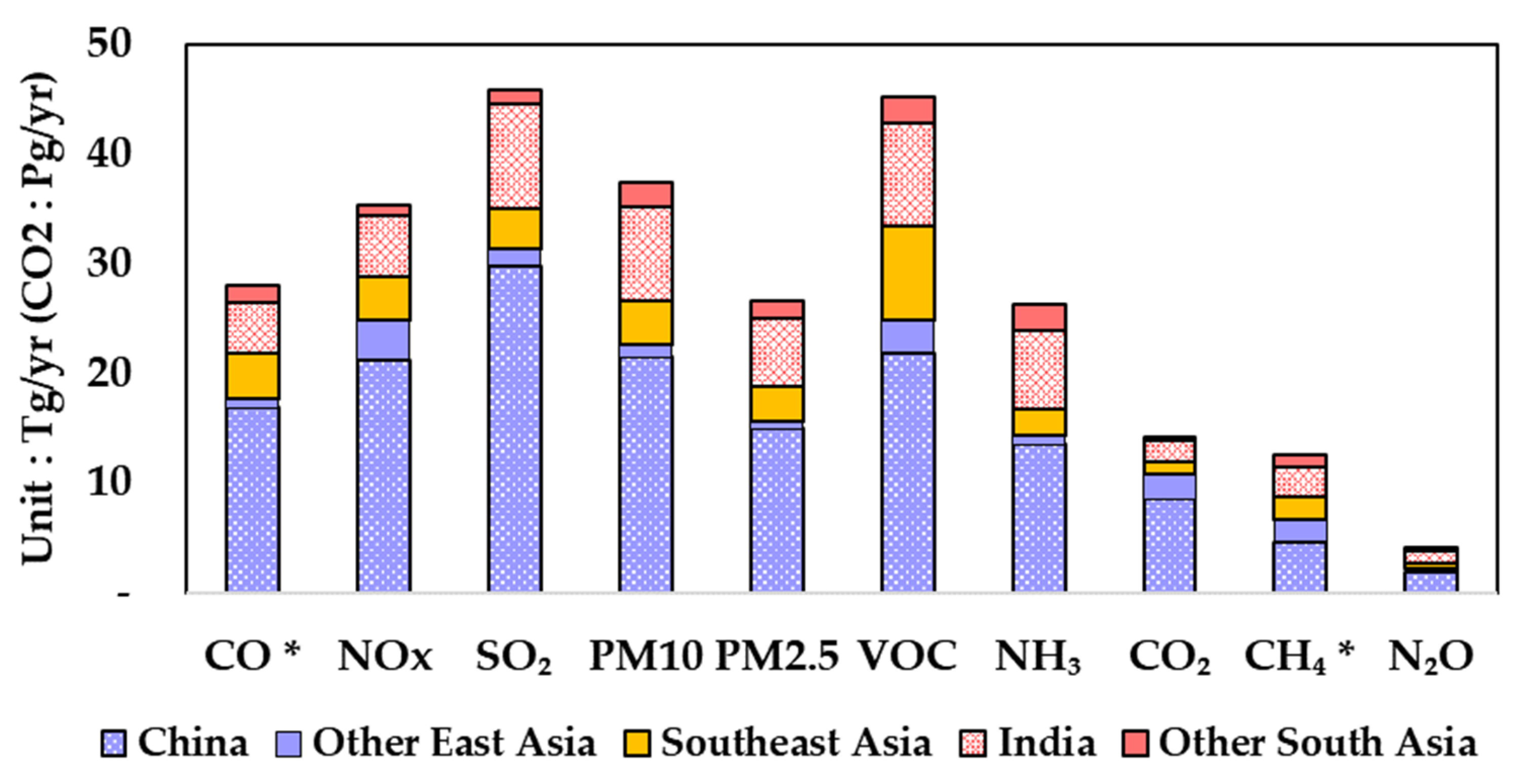
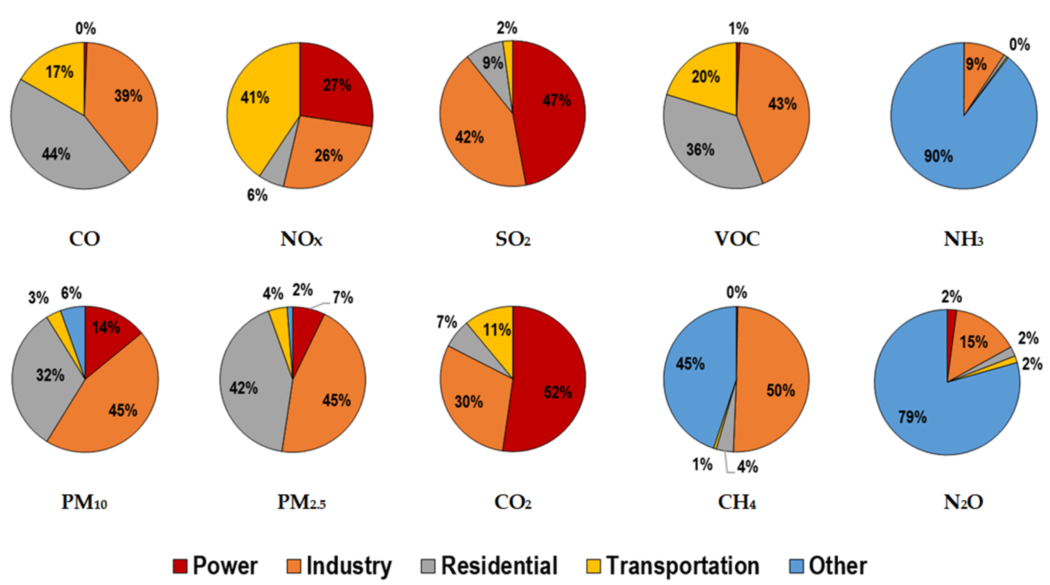
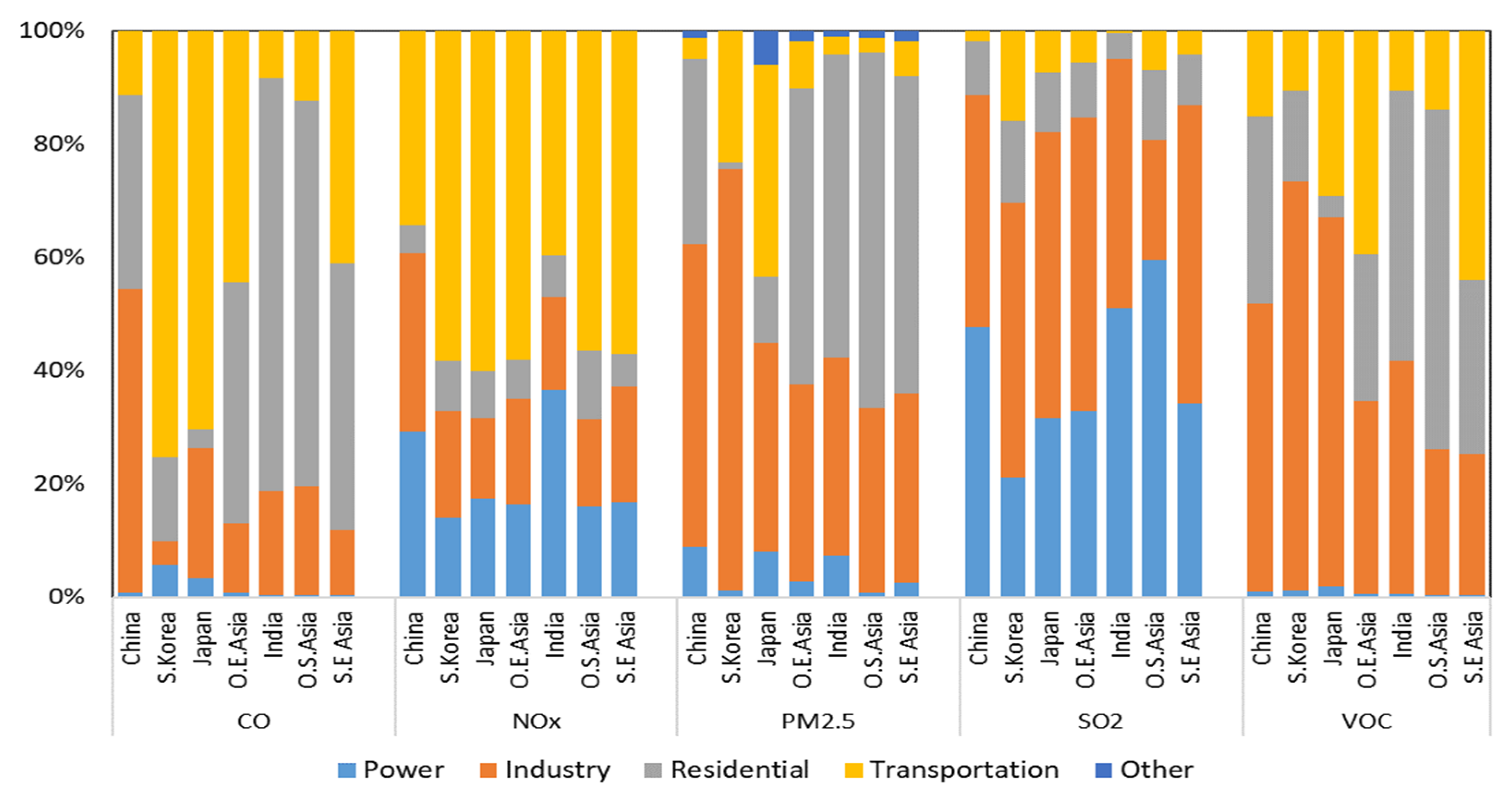
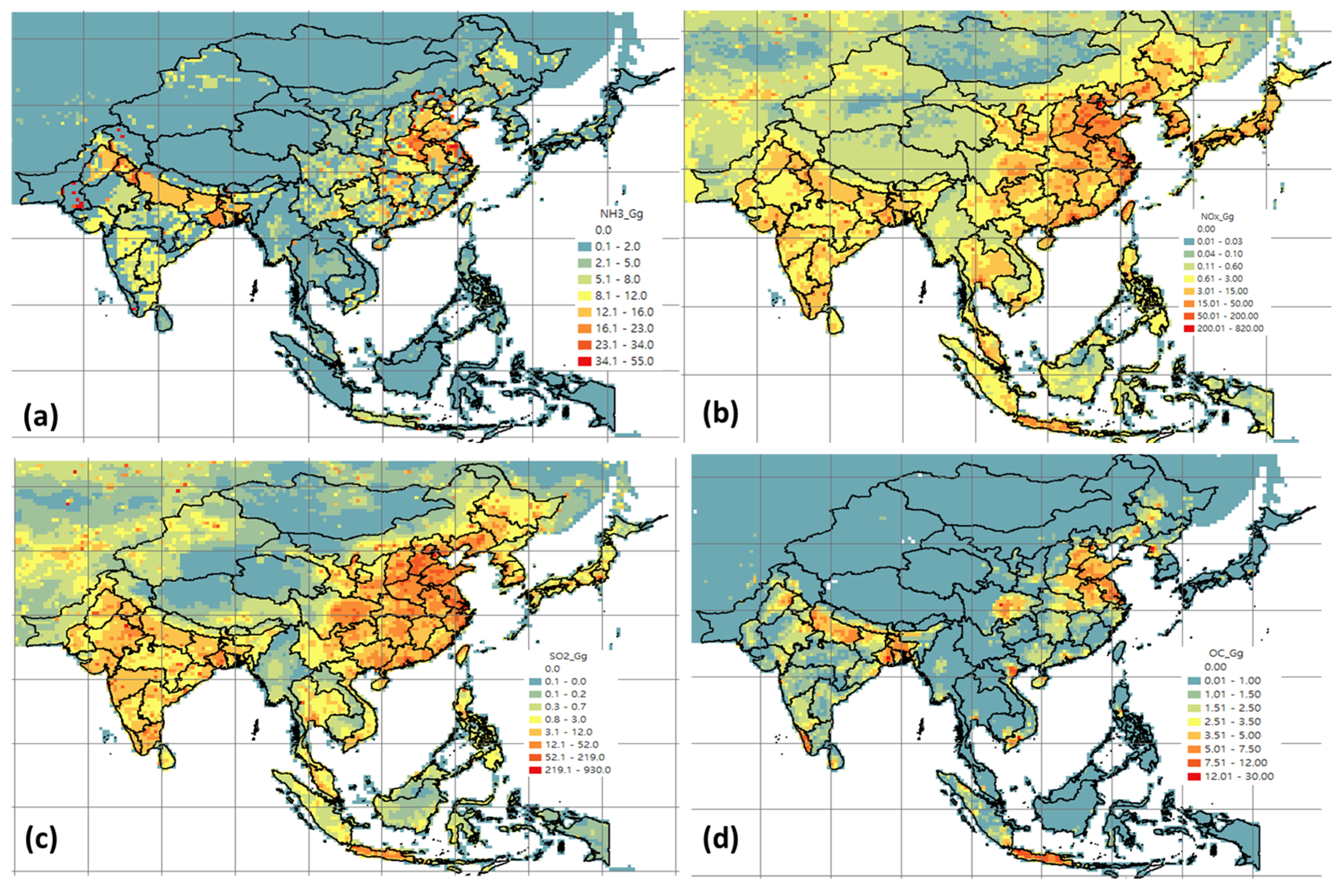
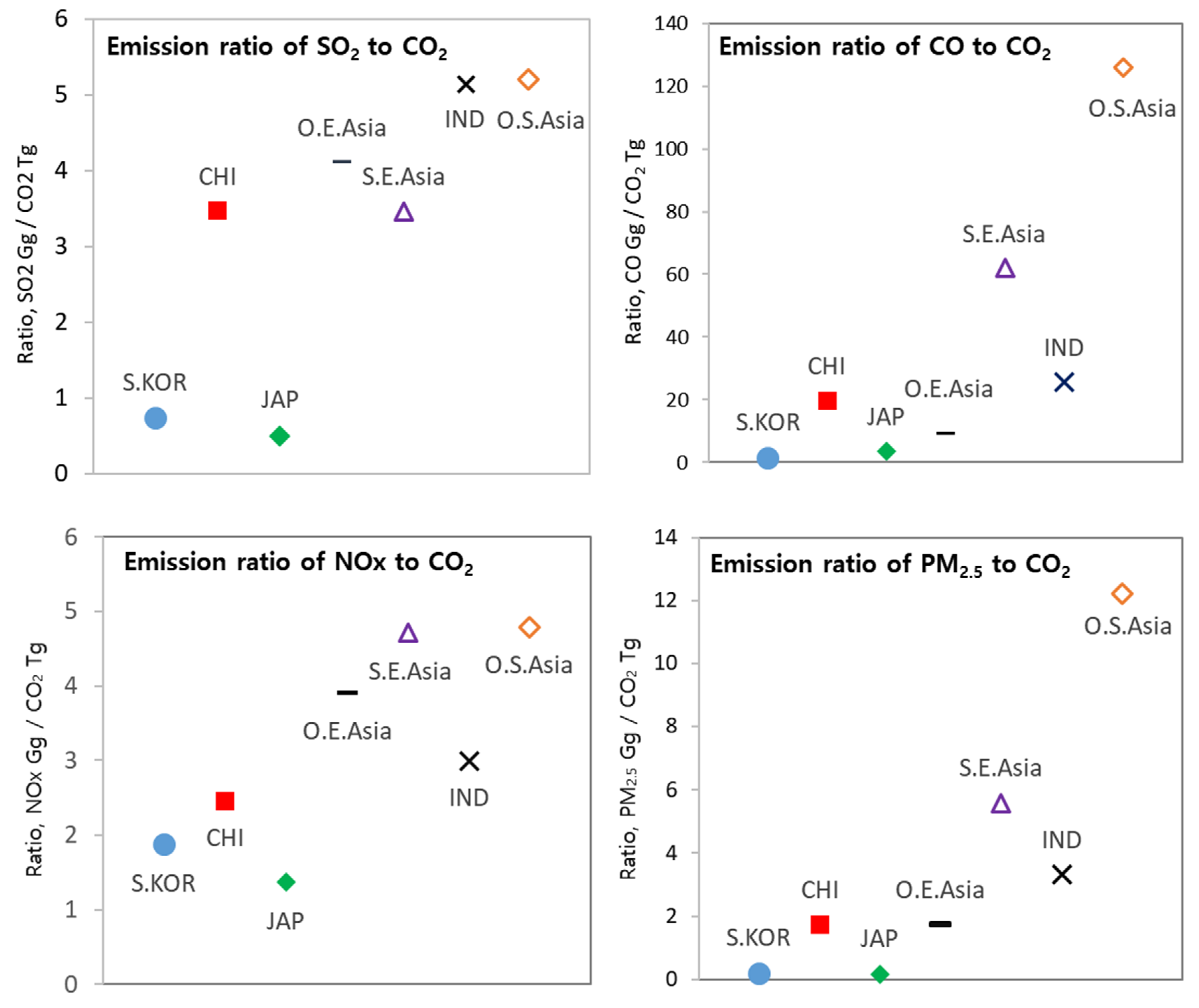
3.1. Asian Anthropogenic Emissions in 2010

National and regional emissions summaries for each major species by sector in 2010 are presented in

Table 5. Anthropogenic Emissions of Asia by region (Unit: Gg/year, CO₂: Tg/year).

Region	CO	NOx	SO2	PM2.5	VOC	NH3	CO2	CH4	N2O
China (PRC)	168,698	21,211	29,855	14,969	21,913	13,492	8611	46,779	2001
Korea(south)	837	1094	402	111	850	269	585	1247	28
Japan	4188	1701	614	175	1414	308	1249	1337	98
Mongolia	64	58	73	19	20	94	8	316	31
Korea (North)	1462	319	318	281	272	80	103	618	16
Taiwan (ROC)	1414	440	139	49	402	121	261	568	18
E. Asia total	176,663	24,823	31,427	15,603	24,870	14,363	10,817	50,866	2192
Brunei	36	16	12	3	41	29	7	62	2
Indonesia	21,019	1578	1632	1539	4121	830	430	8534	238
Cambodia	799	60	28	75	125	74	5	528	10
Laos	357	27	21	32	99	56	4	241	5
Myanmar	2221	82	32	221	337	340	13	2078	49
Malaysia	3239	519	234	151	936	125	208	1010	35
Philippines	3526	316	609	206	883	249	90	1628	54
Singapore	171	129	130	8	77	23	68	53	38
Thailand	3432	859	552	354	907	259	277	2799	72
Vietnam	6240	398	373	604	1017	415	113	3005	82
S. E. Asia Total	41,041	3984	3623	3193	8544	2400	1213	19,937	585
Bangladesh	4770	183	154	486	745	599	44	3866	30
Bhutan	155	9	6	13	29	31	2	104	5
India	47,648	5548	9508	6163	9495	7162	1850	26,975	1002
Sri Lanka	1049	57	67	104	178	44	11	406	12
Nepal	1967	36	47	188	275	189	7	1015	32
Pakistan	7191	688	1132	925	1053	1568	191	6334	227
S. Asia Total	62,780	6521	10,914	7879	11,775	9593	2104	38,699	1308
Total	280,485	35,327	45,963	26,675	45,190	26,356	14,135	109,502	4085

. We estimated total Asian emissions for 2010 as follows: CH₄ 109.4 Tg, CO 280.5 Tg, CO₂ 14.1 Pg, N₂O 4.1 Tg, NH₃ 26.4 Tg, NO_x 35.3 Tg, PM₁₀ 37.4 Tg, PM_2.5 26.7 Tg, SO₂ 46.0 Tg, and VOC 45.2 Tg—with the emission distribution in each Asian regional group shown in Figure 4. E. Asia contributed between 53% and 77% of the total for all Asia, and China’s emissions were predominant in not only E. Asia but also across the entire Asia region. S. Asia contributed approximately 25%, on average, and its emissions were dominated by those from India, which made the second-largest contribution to total Asian emissions, following China. S. E. Asia contributed >15% to the total VOC and CO emissions and ~10% of the other pollutant totals. Apart from India, the other S. Asian countries contributed <5% of the emissions of most pollutants, although these other S. Asian countries contributed approximately 10% of the agriculture-related pollutants total (NH₃, CH₄, and N₂O).

Sectoral emission totals for 2010 for Asia and each region are shown in Figure 5 and Figure 6 respectively. For SO₂, large contributions from coal-fired power plants and the manufacturing industry predominated, with power (47%) and industry (42%) being the largest source sectors in Asia. The figures showed that the power sector was the largest emitter (>50%) in China, India, and other South (OS) Asia, while the industry sector was the largest contributor in S. Korea and Japan. For NO_x, the inventory showed that the power, transport, and industry sectors were important source sectors in all regions. Contrary to SO₂ emissions, other East (OE) Asia and S. E. Asia both accounted for >10%, through the contributions made by their transportation sectors. China and India showed relatively low transportation sector contributions compared with the other regions due to the overwhelming size of their power sector contributions.

For PM_2.5, domestic biofuel and coal consumption was high in India, OS Asia, and S. E. Asia, which explained why the residential sector was the dominant PM_2.5 emissions contributor, while in S. Korea and Japan the industry and transportation sectors were dominant. For CO, the power sector contributed less than it did to other combustion-related species; this reflected the concept that CO is mainly emitted from incomplete combustion, and power plants generally have higher combustion efficiencies than those of either smaller industrial facilities or residential cooking and heating equipment. The data showed that residential sectors were the major CO emitters in most regions, except in S. Korea and Japan. S. Asia, including India, made higher residential sector contributions than other regions, while emissions from transportation were the largest contributor in Japan and S. Korea.

For VOCs, industry, including solvent sources, was the largest source sector in China, S. Korea, and Japan, and was an important source for all VOC species. The residential sector was also a major CO and VOC contributor, with the exceptions of S. Korea and Japan—mainly as biofuel use is very limited in these countries, which focus mainly on gas fuels in the residential sector, in line with the National Institute of Environmental Research (NIER) 2013 [39], and as reported in Ohara et al. [1]. Transportation is an important CO and VOC source sector, especially in S. E. Asia, due to the high numbers of two- and three-wheeled transportation formats there, as reported in F. Posada et al. [40].

NH₃, NO_x, SO₂, and OC emission maps, for 2010, are presented in Figure 7, at a 0.1° × 0.1° grid resolution. These maps show quite clearly that the Indian Indo-Gangetic Plain and the Chinese east coast were high emission areas for all pollutants in 2010. SO₂ emissions from the Chinese east coast and the central west coast of India were very high, while high NO_x emission regions were widely distributed across S. Korea, Japan, China, and India, and around the S. E. Asian megacities. In China, high emission regions included the Northeast and the Yangtze and Pearl River deltas.

We analyzed pollutant-to-pollutant ratios to understand regional emissions characteristics. Anthropogenic CO₂ emission is a good indicator for energy use whereas air pollutants emissions are good indicators for combustion efficiency (CO) and strength of environmental policy-technology measures (NO_x, SO₂). Ratio analyses allow control levels to be deduced.

It was apparent from review of the data mapped in Figure 8 that the SO₂/CO₂, NO_x/CO₂, CO/CO₂, and PM_2.5/CO₂ emission ratios were lower in S. Korea and Japan than in other regions. This perhaps reflected the improved emission control measures—such as FGD devices, for SO₂ control, and selective catalytic reduction (SCR) technologies for NO_x control—operating there. The most significant regional differences were observed for the CO/CO₂ ratio. CO emissions result from low combustion efficiencies in the residential sector. Since solid fuels, such as coal or biofuel, are rarely used for cooking and heating in a residential sector, S. Korea and Japan have low CO emission levels from this sector, with the industry and transportation sectors providing the major CO emission sources in these two countries. In contrast, coal and biofuels provided a high total energy consumption share in the residential sector in S. E. Asia, O.S Asia, and India.

We evaluated the CREATE emission inventory by region, using per-capita and GDP metrics, as population and GDP are major driving forces behind anthropogenic emissions, making these parameters good indicators for emission intensity evaluation. GDP figures provided by the World Bank (in USD), as constant purchasing power parity (PPP) [41], were used, and we compared the top four CO₂ emitters in Asia for the purposes of this analysis.

Review of the estimates shown in Figure 9 indicated that China’s emission per GDP unit was the highest for most pollutants, with the exception of NH3, with its NO_x and SO₂ emissions per GDP unit being noticeably high, which might indicate higher combustion-related activities in various sectors including power generation and industry. For NH3, India was the highest emitter per GDP unit, which was probably reflected a higher level of agricultural and livestock activities. Japan exhibited the lowest emissions per GDP unit for all pollutants, except NO_x, followed by S. Korea.

The data showed quite clearly that S. Korea and Japan had low air pollutant emissions per GDP unit—even with high economic activity—demonstrating that effective emissions control technologies were more often applied in these two countries. This can also be seen in the fact that differences in CO₂ per GDP unit for each country were significantly less than the differences apparent for other pollutant emissions, as CO₂ emissions are mostly dependent on fuel use, rather than on control measures.

Economic development status and industry roles within the global supply train is also a major factor for the differences of ratio. The manufacturing industries with higher energy use and heavier pollution generation tend to migrate from more developed countries to the developing countries to avoid more stringent regulations.

Regional per-capita emissions comparisons, prepared using population data obtained from the World Bank (https://data.worldbank.org/indicator), have been illustrated in Figure 10. The legends O.E.A (for other E. Asia), O.S.A (for other S. Asia), and S.E.A (for S. E. Asia) indicate where the average values represent regional groups. Unlike the per-GDP emissions, S. Korea and Japan show high per-capita NO_x and VOC emissions, with the high S. Korea emissions (compared with other regions) representing the outcome of higher per-capita energy use—in applications such as more cars and industry—which reflects its more advanced economic development. For SO₂ and PM_2.5, China showed the highest per-capita emissions, while for NO_x and NMVOCs China showed levels similar to those of S. Korea and Japan. India showed low per-capita emission levels for all pollutants.

Future per-GDP and per-capita emissions analyses would be expected to show noticeable value changes due to both the ongoing rapid economic growth in India and S. E. Asia and the significant emission reductions achieved by Chinese emissions control policies.

3.2. Natural Emissions

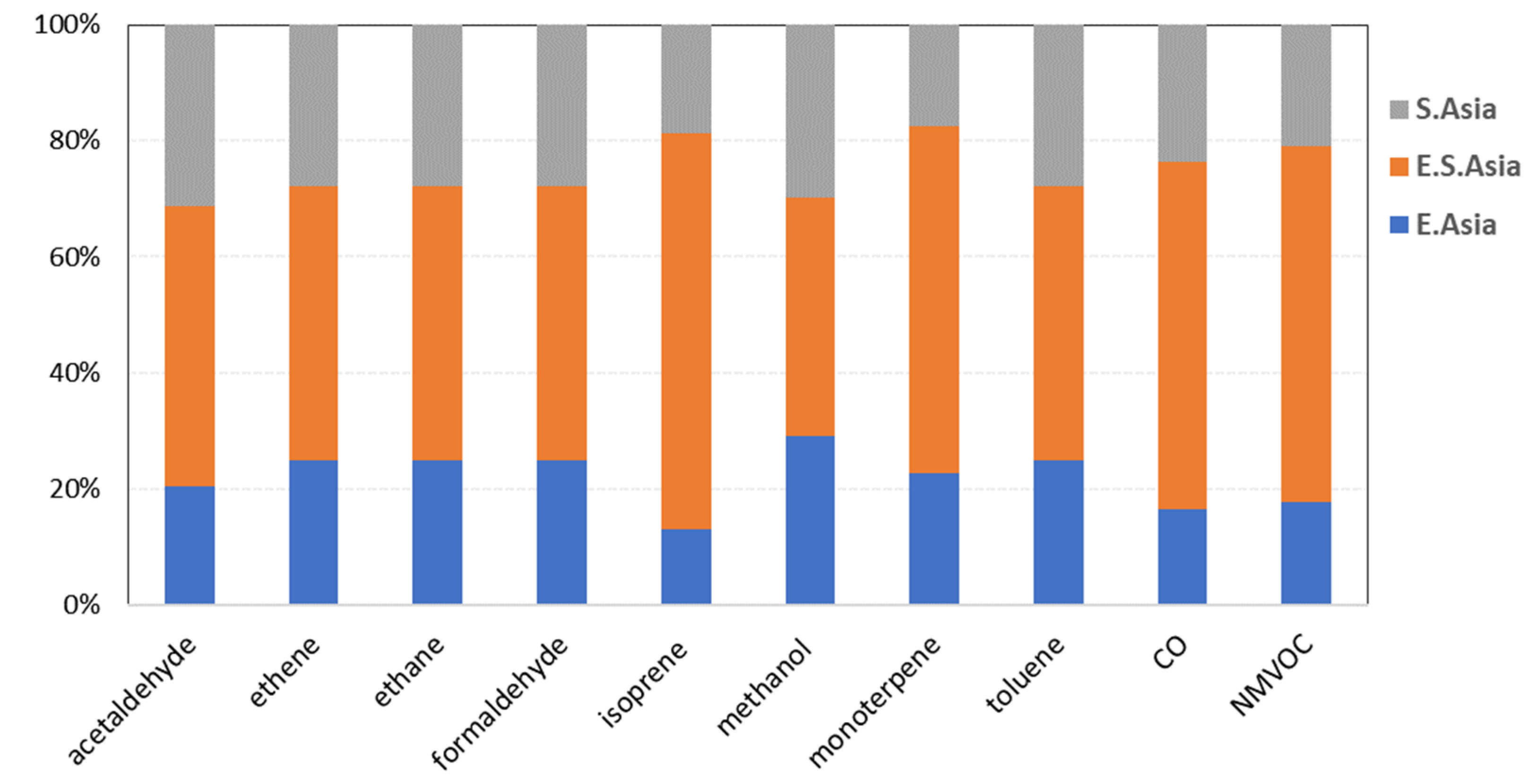
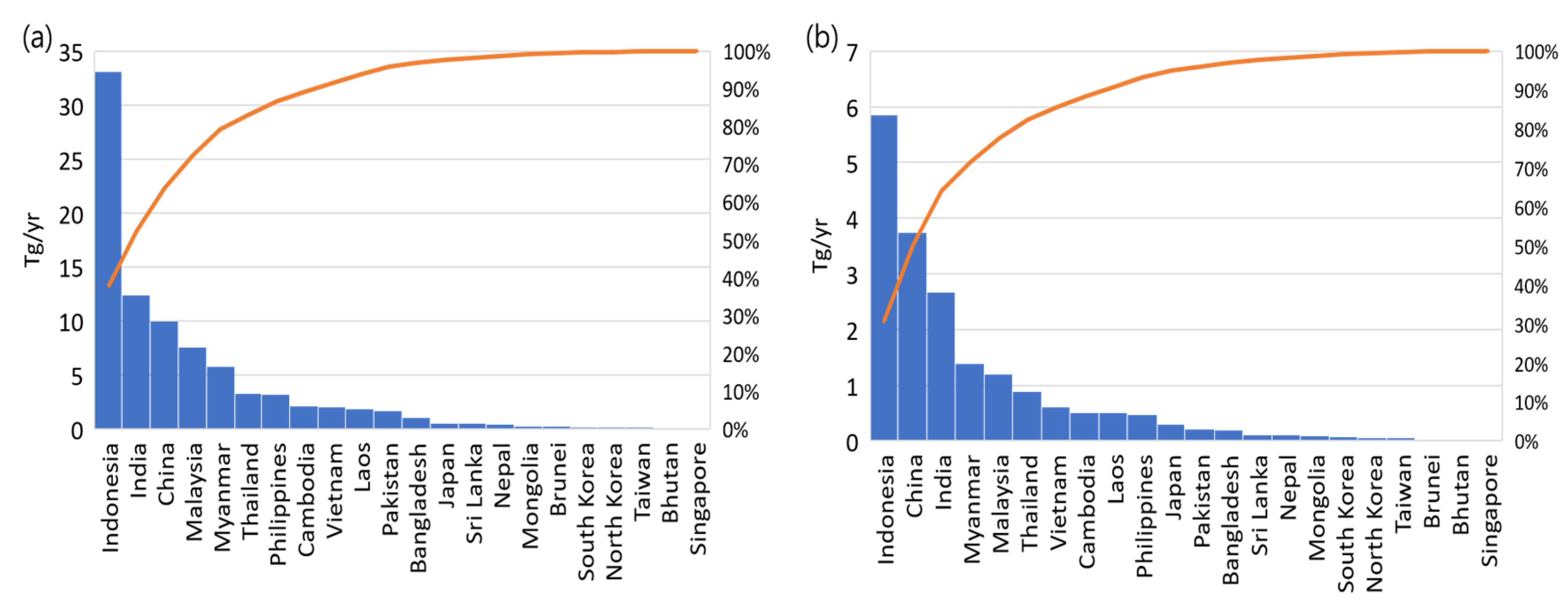
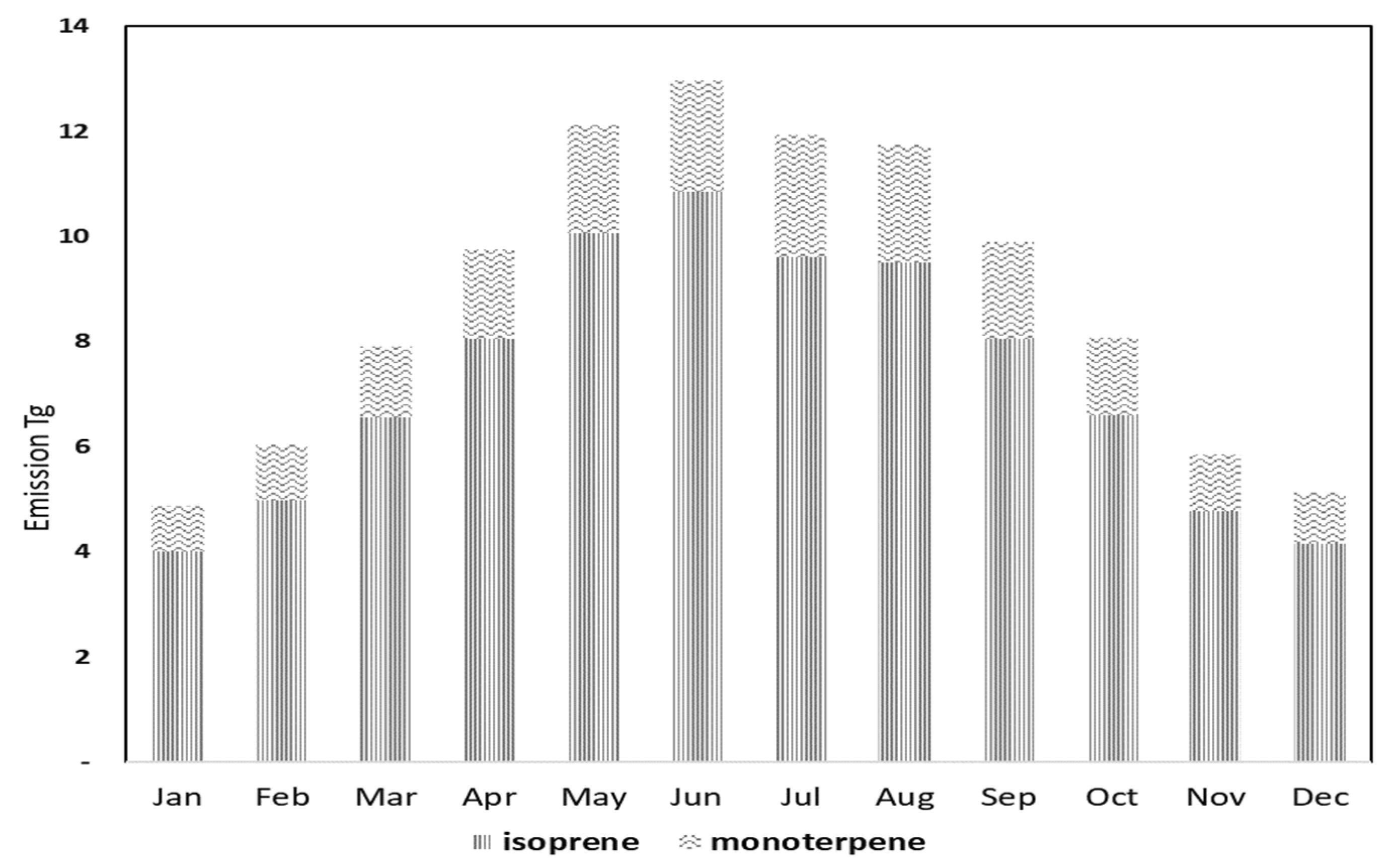
3.2.1. Biogenic Emissions

Monthly mean biogenic emission data for nine major species—isoprene (C₅H₈), monoterpene (C₁₀H₁₆), acetaldehyde (CH₃CHO), carbon monoxide (CO), ethylene (or ethene) (C₂H₄), ethane (C₂H₆), formaldehyde (CH₂O), methanol (CH₃OH), and toluene (C₇H₈)—were estimated for Asia, for 2009, using MEGANv2.04, on a 0.1° × 0.1° grid. Annual totals for these species are listed by country in

Table 6. Biogenic emissions across the countries in Asia (unit: Tg/year).

	Isoprene (C5H8)	Monoterpene (C10H16)
S. Korea	0.20	0.07
N. Korea	0.18	0.06
Japan	0.57	0.31
Taiwan	0.15	0.05
Mongolia	0.28	0.09
China	9.99	3.74
Laos	1.91	0.50
Thailand	3.31	0.90
Vietnam	2.06	0.62
Myanmar	5.83	1.40
India	12.41	2.67
Philippines	3.25	0.47
Bangladesh	1.05	0.19
Bhutan	0.05	0.02
Brunei	0.23	0.03
Cambodia	2.15	0.51
Indonesia	33.15	5.86
Malaysia	7.63	1.20
Nepal	0.45	0.11
Pakistan	1.73	0.22
Singapore	0.01	0.00
Sri Lanka	0.56	0.12
Total	87.14	19.133

.

The biogenic emissions distribution for each Asian regional are shown in Figure 11, which shows that, in contrast to anthropogenic emissions, S. E. Asia contributed the most, emitting from 41 to 68% of the Asian total, while E. Asia made the smallest contribution.

For isoprene (C₅H₈), which accounts for the largest share of vegetation VOCs, the top emitters were Indonesia (33.1 Tg/yr), India (12.4 Tg/yr), China (10.0 Tg/yr), Myanmar (7.6 Tg/yr), and Malaysia (5.8 Tg/yr), followed by the rest of Asia. These five countries accounted for 79% of the Asian biogenic isoprene emissions total.

The top emitters for monoterpene (C₁₀H₁₆), which contributes significantly to secondary fine particulates production through photochemical reactions with isoprene (C₅H₈), were Indonesia (5.9 Tg/yr), China (3.7 Tg/yr), India (2.7 Tg/yr), Myanmar (1.4 Tg/yr), and Malaysia (1.2 Tg/yr), with these five accounting for 77% of the Asian biogenic monoterpene emissions total (Figure 12).

As can be seen in Figure 13, biogenic emissions showed seasonal variations in response to the differing environmental conditions, such as temperature, solar radiation, and precipitation. Figure 14 indicates that isoprene emissions peaked in June, while monoterpenes peaked in July–August. Emissions of both isoprene and monoterpenes were approximately 65% higher in the hot season (April–September) than they were in the cold season (October–March), mainly because their causal factors (such as temperature, solar radiation intensity, and plant distribution density) also peak in summer.

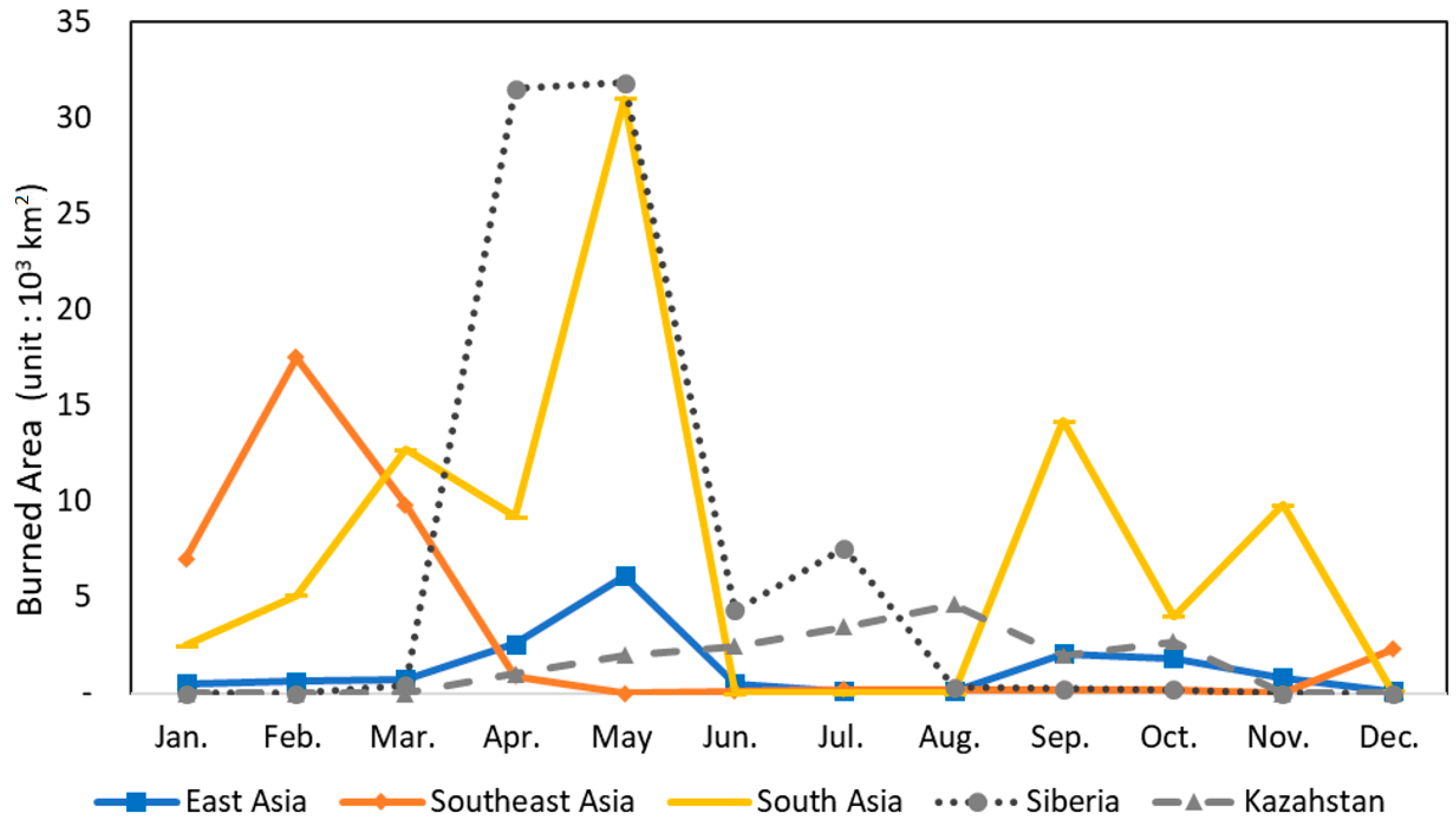
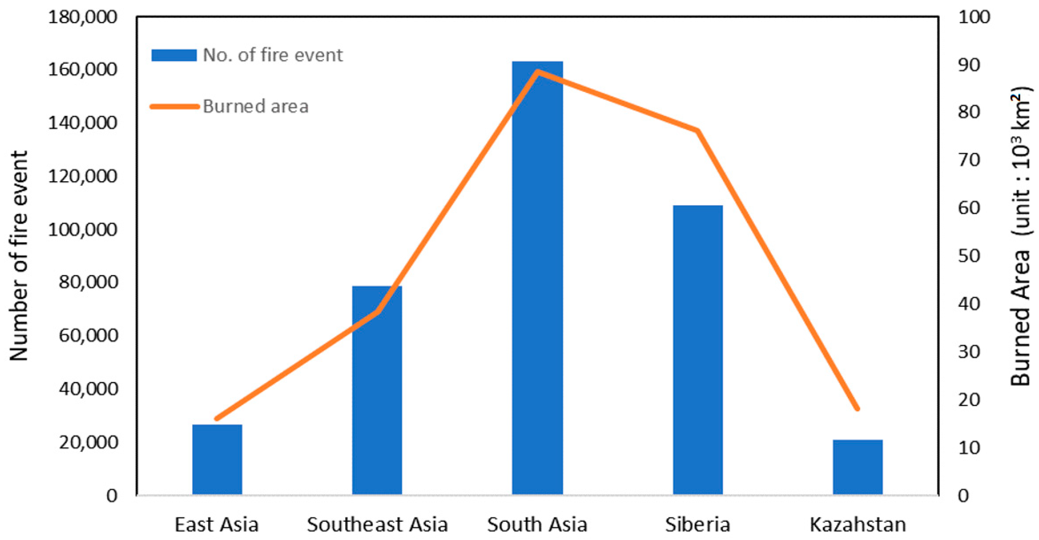
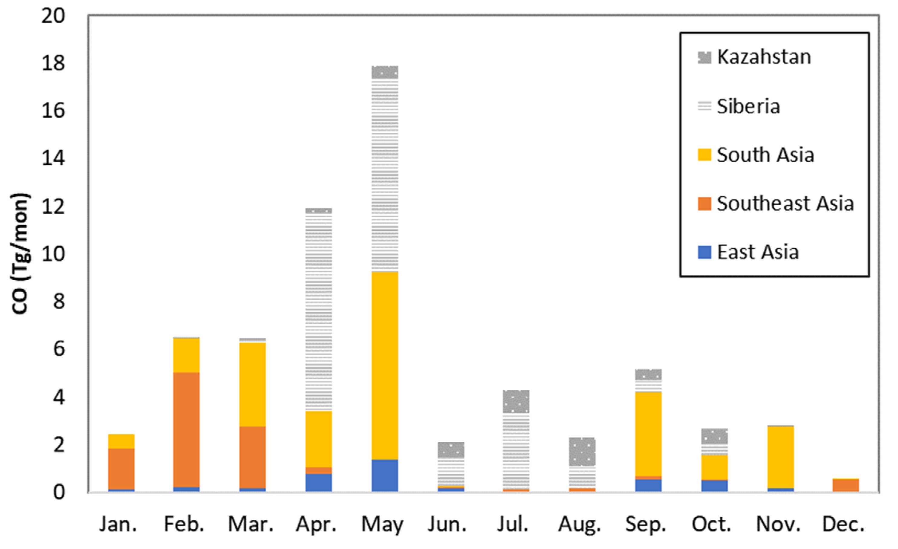
3.2.2. Biomass Burning Emissions

Location emissions estimated using MODIS burned-area data (MCD45A1), https://ladsweb.modaps.eosdis.nasa.gov/ [42]) are shown in Figure 14, where we have summarized January, April, July, and October data as representatives of the four seasons to help explain both the regional and seasonal nature of biomass burning event distribution.

In winter (as represented by Jan. in Figure 15), fewer fire events or burned areas were seen than in spring (April), with those that did occur located south of 25° N, in S. Asia, S. E. Asia, and southern China, and none seen above 30° N.

Compared with other seasons, in spring numerous fire events were apparent, not only in Asia but also in southern Siberia, while in summer (July), the fewest biomass burning events and the smallest biomass burning area occurred. Comparing spring with summer (April and July), the burned areas were much larger in April than they were for July, while for fall (October), the burned area was again observed to be rather high for S. E. Asia. This burned area seasonality generally aligned well with previously published findings [43].

Figure 15 shows that the area burned in spring accounted for 60% of the total. In Asia, the lowest total combustion area occurred in summer (June–August), most likely due to the influence of monsoon cloud formation and significant rainfall. Overall, the largest burned area was seen in spring, peaking in May in E. Asia, and February in S. E. Asia. In S. Asia, significant areas of burning were observed, compared with the other two Asian regions, especially in May. Given that the most populous areas are found in the mid-latitudes, direct human health impacts from biomass burning are likely to be the highest there. In Siberia and Kazakhstan, burned areas regularly appear in summer, contrary to more southern Asian locations, with large and intense burning detected over April and May, concentrated mostly in the Siberian region.

2009 CO, PM_2.5, and nonmethane hydrocarbons (NMHC) emissions from biomass burning are summarized in Table 6, by subregion, total annual Asian emissions, and by emissions totals for all Asian regions.

Total 2009 Asian CO emissions from biomass burning were 37.6 Tg, with S. Asia contributing 61% (23 Tg), S. E. Asia 28% (10.4 Tg), and E. Asia 11% (4.1 Tg). Total Asia emissions accounted for 59% of the study area, with S. Asia being the largest contributor, not only in Asia but across the whole domain. Siberia made the second highest contribution, followed by S. Asia, which accounted for >30% of the whole domain. E. Asia made the smallest contribution at 5–7% of the whole domain (

Table 7. Summary of emissions from biomass burning for the year 2009 (Tg/year).

	East Asia	Southeast Asia	South Asia	Siberia	Kazakhstan	Total
PM2.5	0.5	1.2	2.7	2.4	0.6	7.3
CO	4.1	10.4	23.0	22.8	4.7	65.0
NMHC	0.1	0.3	0.8	0.7	0.2	2.2

). As illustrated in Figure 16, these results correlated strongly with the burned areas and fire event numbers.

Monthly sub-regional CO emissions from biomass burning are shown in Figure 17, which shows that in the target year these emissions were concentrated between February and May in Asia, while becoming significantly reduced in June and August, due to weather conditions such as rainfall and humidity. In the fall, from September to November, biomass burning emissions increased again, although at a lower level than in spring. Overall, the highest emissions occurred in May, presumably from S. Asian locations such as India, while Siberia and S. Asia contributed approximately 49% and 44%, respectively. In April, ~75% of the emissions appeared from the Siberian region, and in Asia, as in May, the highest contribution came from S. Asia, at ~20%, which was lower than May. From January–March, Siberian contributions were rare, with most emissions occurring in Asia. Overall, these monthly emission variations showed patterns very similar to those seen for both the areas burned and fire event numbers.

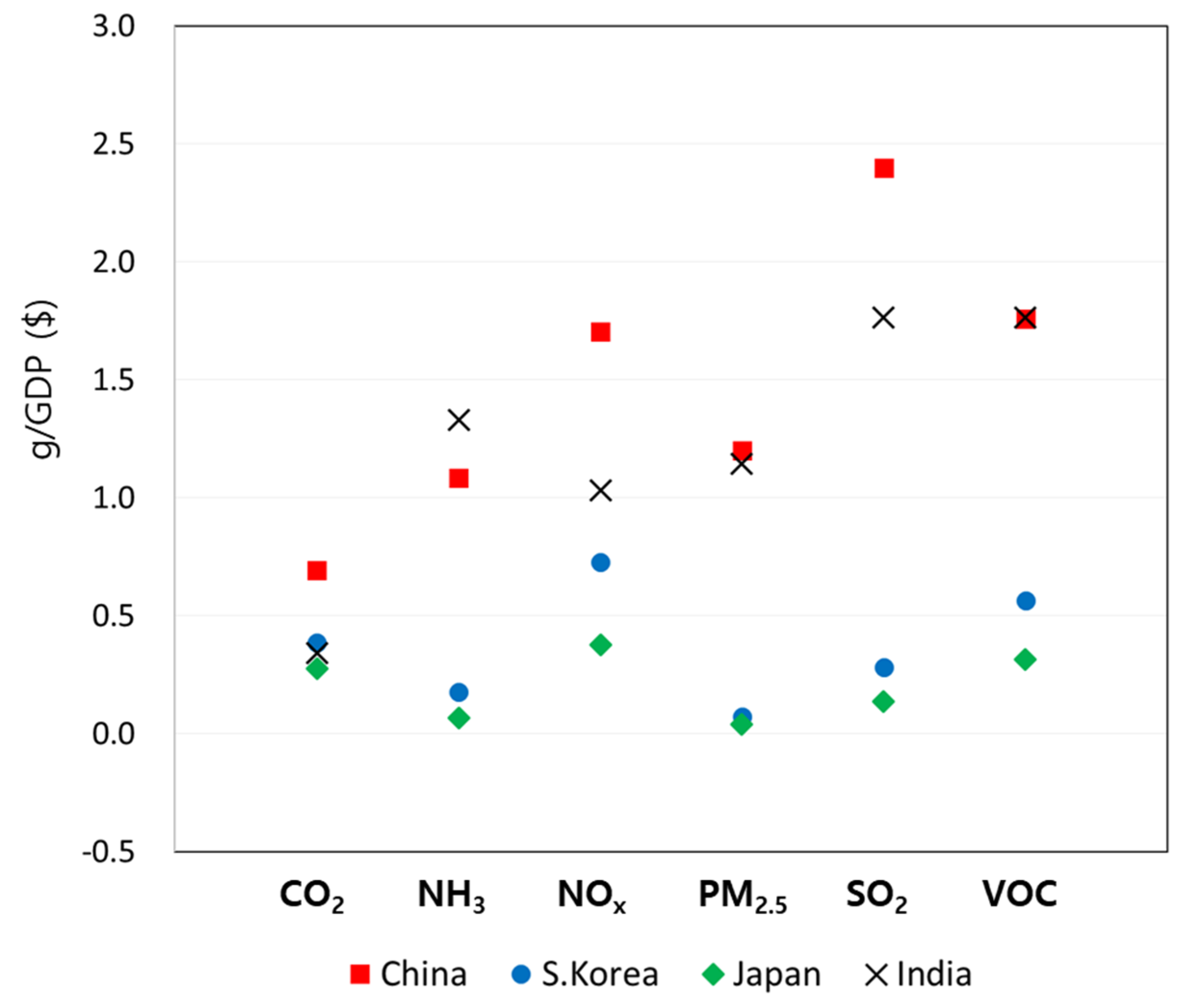
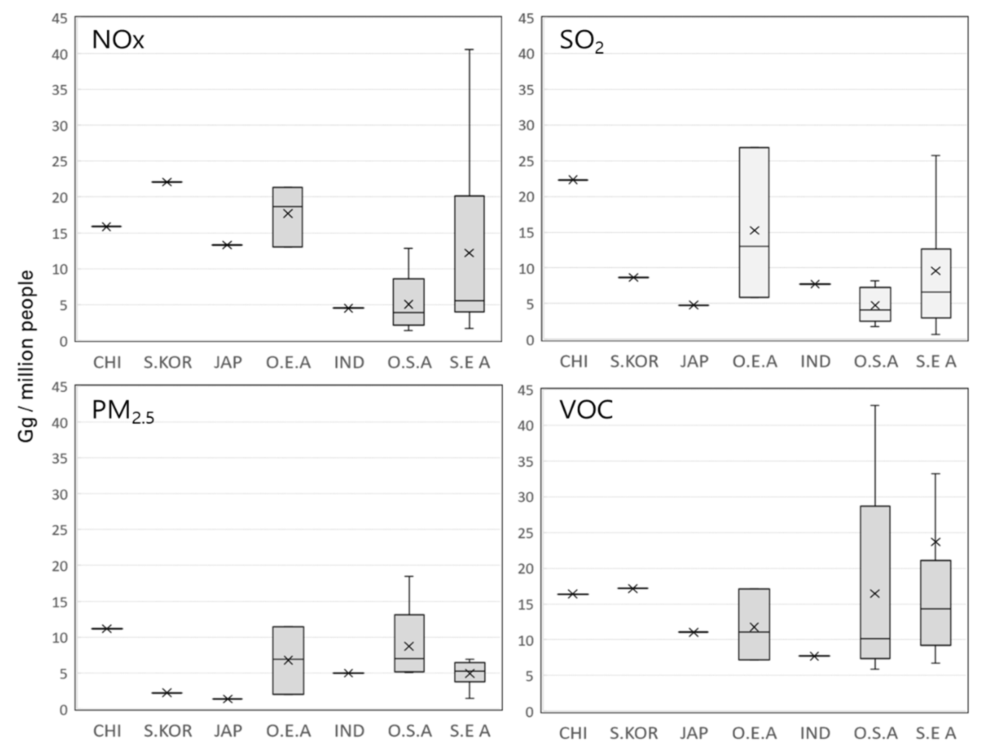
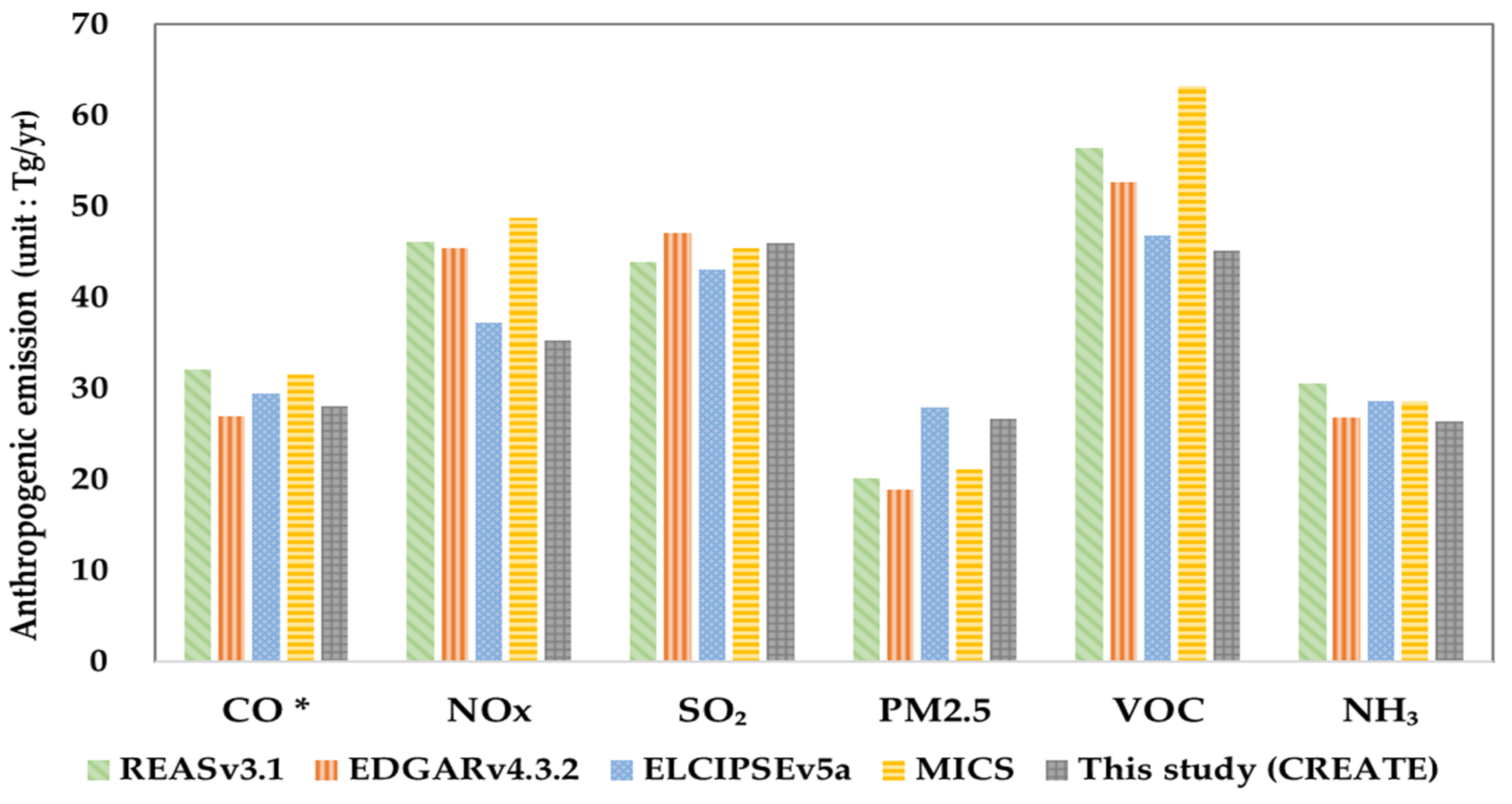
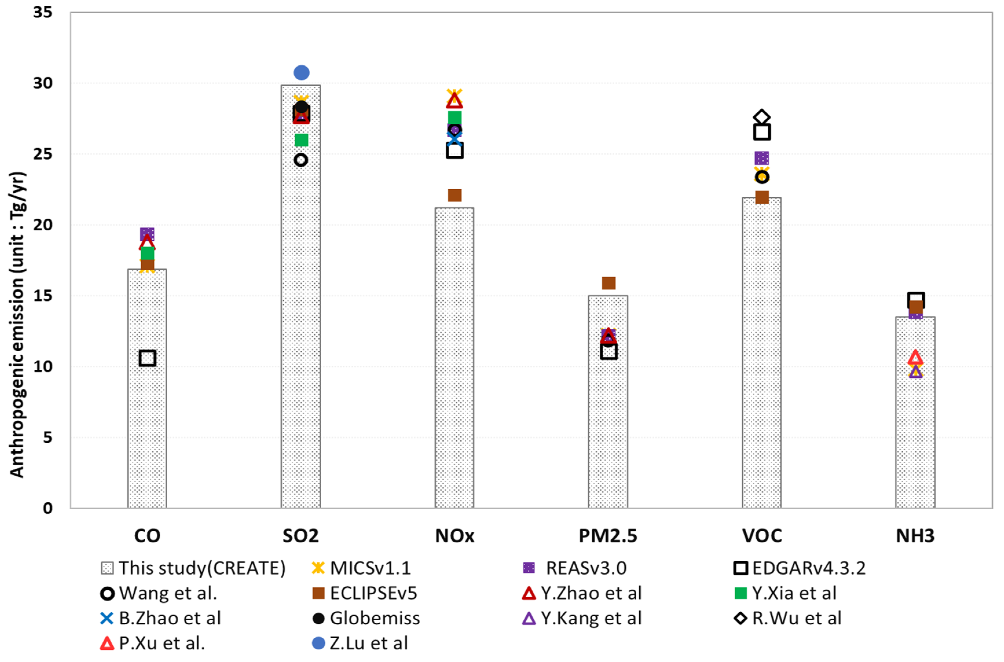
3.3. Comparisons between This Study and Other Emissions Datasets

To better understand differences among anthropogenic emission estimates, we reviewed total emissions estimate differences for Asia, calculated for the same base year as this study. To do this, we compared the CREATE inventory outcomes with those produced by the REAS v3.1 (Regional Emissions Inventory in ASia v3.1) [44], MICS (the Model Inter-Comparison Study for Asia) [45], ECLIPSE v5a [46], and EDGAR v4.3.2 [47] inventories (Figure 18). We found that the all-Asia CO, SO₂, and NH₃ emissions estimates from CREATE showed a range similar to those of the other inventories, although NO_x and VOC estimates averaged 26% and 21% lower, respectively, and the CREATE PM_2.5 estimates were 17% higher. The largest difference in the emissions ranges, of 80–139% across the various pollutants, was found between the CREATE and MICS inventories. We found that the ECLIPSE model produced values that were the closest to CREATE; this was not unexpected, as both inventories were based on the GAINS model, had the same source categories and used the same emissions factors, with the exceptions of China, N. Korea, and S. Korea.

In Figure 19, we can see a comparison between CREATE inventory emissions for China with those from previous studies, with CREATE represented by the black bar with a check pattern and other inventories indicated by variously marked dots. The figure shows that for CO, the CREATE results were 1–14% lower than those from the other inventories, apart from EDGAR, whose CO emission estimate were much lower (37–45%) than those from the other studies. For SO₂, the CREATE estimate was high, at 29.85 Tg, which was 4–17% above estimates from the other inventories, apart from that from Lu et al. [48], which was 3% lower.

We found that CREATE NO_x emission estimates were 11–37% lower than those from the other inventories, exhibiting the lowest values. There were greater differences between the various inventories for NO_x, VOC, and NH₃ than there were for the other emission species, while the MICS CO and SO₂ emissions estimates showed good agreement (within 3%) with those from CREATE, although large differences were apparent between the two inventories with respect to their NO_x and VOC emissions estimates. These latter differences may be showing how local NO_x and VOC studies captured Chinese domestic information that was more accurate and were thus better able to reflect increases in car use, industrial source emissions, and solvent usage there.

We found that the ECLIPSE VOC emission estimate was in very good agreement with that of CREATE (within 0.3%), with all other emissions estimates also in good agreement (within 5%). Compared with inventories other than ECLIPSE, the CREATE PM_2.5 emission estimate was much higher. While for NH₃, two distinct groups were apparent, with REAS, ECLIPSE, and EDGAR showing relatively good agreement with CREATE (all <8% difference), and MICS, Kang et al. [49], and Xu et al. [50], showing much larger differences (all >21% difference). There were also differences of >30% between these two groups.

A comparison between the biogenic emission estimates calculated in this study with previously published estimates is presented in Table 7. The annual Asia isoprene estimate from CREATE was 87.1 Tg, which was between −4% and 39% of the other studies. The CREATE isoprene emission estimate was closest to those published in Stavrakou et al. (2014), and the differences for China were smaller (within 8%) than they were for the rest of Asia. The main reason for the larger differences might be either the use of different model frameworks or different MEGAN versions for emission calculations. Vegetation information (such as vegetation cover and leaf area), meteorological data, and EFs make up the input parameters for biogenic emission modeling, and the specific algorithms for BVOC compound species relate their emissions to surrounding weather conditions. This suggests that there might be differences in EFs and estimation algorithms between each model. We also noted that different target years were used, suggesting that input weather conditions and vegetation information may have differed, which could give rise to emissions discrepancies. Wang et al. [56] reported that meteorological conditions, particularly temperature and solar radiation, could affect isoprene estimates by up to 27% and 51%, respectively.

For monoterpenes, our emission estimates were approximately 18% and 23% higher for Asia and China, respectively, compared with the other inventories, although the China monoterpene emission estimate in Klinger et al. (2002) was in very good agreement (within 0.1%) with that achieved using CREATE (

Table 8. Inter-comparison of biogenic emissions for China and Asia with other studies [unit: Tg/yr].

Isoprene [Tg/yr]	Asia	China	Monoterpene [Tg/yr]	Asia	China
Guenther et al. (2012) [29]	62.7	9.3	Guenther et al. (2012) [29]	16.2	2.8
Guenther et al. (2006) [28]	81.7	10.9	Y. Fu et al. (2012) [57]		3.0
T. Stavrakou et al. (2014) [58]	90.4	9.3	Klinger et al (2002) [59]		3.7
Y. Fu et al. (2012) [57]		10.9	This study (CREATE)	19.1	3.7
This study (CREATE)	87.1	10.0

).

An inter-comparison between biomass burning emission estimates from this study with those from the Global Fire Emissions Database, Version 4 (GFEDv4) inventory [60,61] and Kaiser et al. [62] was used. The GFEDv4 estimates consist of an average for 2000–2009, while those from Kaiser et al. cover the period 2003–2008. The estimates from this study were higher than those from GFEDv4 and lower than those in Kaiser et al., with the CO emission estimates being 5% higher than those in GFEDv4, and 9% lower than those in Kaiser et al. For PM_2.5, our emission estimates were approximately 10% and 3% higher compared with GFEDv4 and Kaiser et al., respectively. Our result agreed within ±10%, compared to other inventories.

3.4. Uncertainties and Limitations

The emissions used to derive bottom-up anthropogenic inventory estimates were assembled from a variety of human statistics data sources. Generally, such documentation is published with a time lag of several years, while the pace of change in many Asian countries has been increasing, leading to rapid economic development and increasing efforts at mitigating air/climate pollutant emissions. These rapid emission changes make it difficult to maintain emission input statistic currency and to reflect the rapid changes happening in Asia—which in turn leads inevitably to a degree of uncertainty in the representativeness of data. In addition, some countries—such as N. Korea—publish very limited amounts of data, so that, overall, data reliability constitutes a source of uncertainty and limitation for this study.

Biogenic emission estimation is highly dependent on vegetation-related parameters and weather conditions. As mentioned in Section 3.3, using different modeling frameworks or versions (of MEGAN, for example) can cause discrepancies in emission calculations. Henrot et al. [63] also noted that most discrepancies between model calculations could be attributed to meteorological parameter inputs and to LAI and PFT distributions, which can be the source of major uncertainties. This implies that input parameters need to be subjected to appropriate sensitivity testing and should be sampled over longer time periods where possible to support more accurate estimate calculations. Rapid economic development and urbanization throughout Asia continue to cause landcover and land use changes, which also add to emission estimate accuracy uncertainty.

Biomass burning emission estimates can be strongly affected by both fire observation information and burned area size estimates. This means that natural source emissions, from both biogenic sources and biomass burning, include uncertainties related to both meteorological variables and to remote-sensing data uncertainty. Satellite observations are sometimes affected by cloud contamination, for example, as described in Streets et al. [43].

Anthropogenic emissions inventory was estimated based on annual energy statistics, policy measures, and emissions factors whereas natural emissions were estimated using comprehensive emission models with a much more diverse set of input data. Some of the input parameters of the natural emission models were not available for the same period as the anthropogenic emission input data. The base year of natural emissions is a year older than anthropogenic because of the data limitation during the development period. We will use the same base year for every emission source in our new development of the inventory.

These issues will form part of our future research focus, which will aim to update and improve the work described here. We need to continue our evaluation experiments by including more ambient data observations, and by updating and improving CREATE emission data, in order to build on the outcomes achieved so far in this study.

3.5. Data Availability

We have launched a data download platform for the CREATE inventory at http://aisl.konkuk.ac.kr/#/emission_data/create_emission_inventory. Monthly gridded emission data sets for each major sector, at 0.1° × 0.1° resolution for Asia, and 3 × 3 km resolution for S. Korea, can be downloaded for all species. Data provenance information and a summary table of annual emissions by sector can also be accessed.

4. Summary and Conclusions

We developed a new regional emissions inventory, named CREATE (Comprehensive Regional Emissions Inventory for Atmospheric Transport Experiment). This was designed as a comprehensive emissions framework, including both anthropogenic, biogenic, and biomass burning emissions estimates. Since the emissions in CREATE were estimated based on human and natural activities, both static databases and dynamic models had to be broadly applied in the framework, and then integrated into the final inventory database. The target species in this work included major air pollutants and GHGs, with estimates calculated for both national and regional emissions.

Anthropogenic emissions were developed using the GAINS-Asia framework, which is an integrated policy assessment model. Major activity data were sourced from official national or international statistics to estimate anthropogenic emission totals in CREATE, while EFs and data on the degree of control equipment penetration (such as FGD and SCR) were updated using published literature and government reports.

Our final estimates for Asian total anthropogenic emissions in 2010 were as follows: CH₄—109.4 Tg; CO—280.5 Tg; CO₂—14.1 Pg; N₂O—4.1 Tg; NH₃—26.4 Tg; NO_x—35.3 Tg; PM₁₀—37.4 Tg; PM_2.5—26.7 Tg; SO₂—46.0 Tg; and VOCs—45.2 Tg.

Estimates for nine biogenic emissions in 2009 were calculated, using the MEGAN modeling framework. The model estimates for isoprene emissions in Asia were 87.1 Tg/yr, with 19.3 Tg/yr estimated for monoterpenes. Indonesia, China, and India together accounted for 64% of Asian biogenic emissions.

Biomass-burning emissions in the CREATE inventory were calculated for 2009 using the BlueSky model. We adapted this model for Asia, developing a BlueSky-Asia modeling system, combining this with SMOKE-Asia [7], which is an emission processing system. Modeling outputs were generated as speciated, three-dimensional, model-ready input data for AQ modeling. Total Asia CO emissions from biomass burning were estimated to be 37.6 Tg in 2009; S. Asia contributed 61% (23 Tg) of this total, S. E. Asia 28% (10.4 Tg), and E. Asia 11% (4.1 Tg). We found that the results were strongly influenced by the amount of area burned and by the number of fire events.

CREATE emissions estimates were established for anthropogenic, biogenic, and biomass burning emissions using the same domain, resolution, and period. Final inventory estimates were based on activities and other parameters, which formed fundamental information for the resulting emissions. These characteristics allow CREATE emissions to be applied to many research areas, such as future emission projections, policy-based reduction scenarios, and CC-driven emissions changes. Since SMOKE-Asia, MEGAN, and BlueSky-Asia are either members or linked components of the CREATE inventory framework, its format could be easily adapted to chemical transport modeling. It also can be useful for N. E. Asian studies, as its base year (2010) was an important turning point in emissions reduction, as noted in Woo et al. [64] and Zheng et al. [65].

We believe that our work successfully fulfilled our objective, which was to develop an inventory scheme that provides better support for AQ modeling and which can be operated in concert with the SMOKE-Asia emissions processing system. We hope that the CREATE emissions inventory presented in this paper will contribute to a better understanding of regional air pollution and its influence on human health and climate. We also hope it will provide a basis for future environmental policies and will contribute to international cooperation in the field of regional policy analysis and support. We plan to continue updating and improving the CREATE inventory framework developed in this study.

References

1. Ohara, T.; Akimoto, H.; Kurokawa, J.; Horii, N.; Yamaji, K.; Yan, X.; Hayasaka, T. An Asian emission inventory of anthropogenic emission sources for the period 1980–2020. Atmos. Chem. Phys. 2007, 7, 4419–4444. [Google Scholar] [CrossRef] [Green Version]
2. Kurokawa, J.; Ohara, T.; Morikawa, T.; Hanayama, S.; Janssens-Maenhout, G.; Fukui, T.; Kawashima, K.; Akimoto, H. Emissions of air pollutants and greenhouse gases over Asian regions during 2000–2008: Regional Emission inventory in ASia (REAS) version 2. Atmos. Chem. Phys. 2013, 13, 11019–11058. [Google Scholar] [CrossRef] [Green Version]
3. Jang, Y.; Lee, Y.; Kim, J.; Kim, Y.; Woo, J.-H. Improvement China Point Source for Improving Bottom-Up Emission Inventory. Asia Pac. J. Atmos. Sci. 2019, 56, 107–118. [Google Scholar] [CrossRef]
4. Streets, D.G.; Bond, T.C.; Carmichael, G.R.; Fernandes, S.D.; Fu, Q.; He, D.; Klimont, Z.; Nelson, S.M.; Tsai, N.Y.; Wang, M.Q. An inventory of gaseous and primary aerosol emissions in Asia in the year 2000. J. Geophys. Res. Atmos. 2003, 108. [Google Scholar] [CrossRef]
5. Zhang, Q.; Streets, D.G.; Carmichael, G.R.; He, K.B.; Huo, H.; Kannari, A.; Klimont, Z.; Park, I.S.; Reddy, S.; Fu, J.S.; et al. Asian emissions in 2006 for the NASA INTEX-B mission. Atmos. Chem. Phys. 2009, 9, 5131–5153. [Google Scholar] [CrossRef] [Green Version]
6. Olivier, J.G.J.; Van Aardenne, J.A.; Dentener, F.J.; Pagliari, V.; Ganzeveld, L.N.; Peters, J.A.H.W. Recent trends in global greenhouse gas emissions: Regional trends 1970–2000 and spatial distributionof key sources in 2000. Environ. Sci. 2005, 2, 81–99. [Google Scholar] [CrossRef] [Green Version]
7. Woo, J.-H.; Choi, K.-C.; Kim, H.K.; Baek, B.H.; Jang, M.; Eum, J.-H.; Song, C.H.; Ma, Y.-I.; Sunwoo, Y.; Chang, L.-S.; et al. Development of an anthropogenic emissions processing system for Asia using SMOKE. Atmos. Environ. 2012, 58, 5–13. [Google Scholar] [CrossRef]
8. Amann, M.; Bertok, I.; Borken, J.; Chambers, A.; Cofala, J.; Dentener, F.; Heyes, C.; Hoglund, L.; Klimont, Z.; Purohit, P.; et al. A tool to combat air pollution and climate change simultaneously. In GAINS-Asia Methodology Report; IIASA: Laxenburg, Austria, 2008. [Google Scholar]
9. World Energy Statistics. Available online: https://www.iea.org/subscribe-to-data-services/world-energy-balances-and-statistics (accessed on 31 July 2020).
10. China Industry Research Reports Data. Available online: http://www.chinairr.org/ (accessed on 24 July 2020).
11. National Air Pollutants Emission Service. Available online: http://airemiss.nier.go.kr/mbshome/mbs/airemiss/index.do (accessed on 2 April 2020).
12. Statistics Bureau of Japan. Available online: http://www.stat.go.jp/english/data/nenkan/index.html (accessed on 31 March 2020).
13. United Nations Statistics. Available online: https://unstats.un.org/unsd/energystats/data/ (accessed on 8 January 2020).
14. Zhao, B.; Wang, S.; Liu, H.; Xu, J.Y.; Fu, K.; Klimont, Z.; Hao, J.M.; He, K.B.; Cofala, J.; Amann, M. NOx emissions in China: Historical trends and future perspectives. Atmos. Chem. Phys. 2013, 13, 9869–9897. [Google Scholar] [CrossRef] [Green Version]
15. Huo, H.; Yao, Z.; Zhang, Y.; Shen, X.; Zhang, Q.; He, K. On-board measurements of emissions from diesel trucks in five cities in China. Atmos. Environ. 2012, 54, 159–167. [Google Scholar] [CrossRef]
16. Zhao, Y.; Wang, A.S.; Chris, P.; Nielsen, B.; Li, X.A.; Hao, J. Establishment of a database of emission factors for atmospheric pollutants from Chinese coal-fired power plants. Atmos. Environ. 2010, 44, 1515–1523. [Google Scholar]
17. Lei, Y.; Zhang, Q.; Nielsen, C.; He, K. An inventory of primary air pollutants and CO2 emissions from cement production in China, 1990–2020. Atmos. Environ. 2011, 45, 147–154. [Google Scholar] [CrossRef]
18. Zhao, Y.; Chris, P.; Nielsen, M.; McElroy, B.; Zhang, L.; Zhang, J. CO emissions in China: Uncertainties and implications of improved energy efficiency and emission control. Atmos. Environ. 2012, 49, 103–113. [Google Scholar] [CrossRef]
19. GAINS-Online. Available online: http://gains.iiasa.ac.at/index.php/home-page/241-on-line-access-to-gains (accessed on 31 August 2020).
20. Kota, S.H.; Schade, G.; Estes, M.; Boyer, D.; Ying, Q. Evaluation of MEGAN predicted biogenic isoprene emissions at urban locations in Southeast Texas. Atmos. Environ. 2015, 110, 54–64. [Google Scholar] [CrossRef]
21. Kim, H.-K.; Song, C.-K.; Han, K.M.; Eo, Y.D.; Song, C.H.; Park, R.; Hong, S.-C.; Kim, S.-K.; Woo, J.-H. Impact of biogenic emissions on early summer ozone and fine particulate matter exposure in the Seoul Metropolitan Area of Korea. Air Qual. Atmos. Health 2018, 11, 1021–1035. [Google Scholar] [CrossRef]
22. Wu, K.; Yang, X.-Y.; Chen, D.; Gu, S.; Lu, Y.; Jiang, Q.; Wang, K.; Ou, Y.; Qian, Y.; Shao, P.; et al. Estimation of biogenic VOC emissions and their corresponding impact on ozone and secondary organic aerosol formation in China. Atmos. Res. 2020, 231, 104656. [Google Scholar] [CrossRef]
23. Guenther, A.; Hewitt, C.N.; Erickson, D.; Fall, R.; Geron, C.; Graedel, T.; Harley, P.; Klinger, L.; Lerdau, M.; McKay, W.A.; et al. A global model of natural volatile organic compound emissions. J. Geophys. Res. Atmos. 1995, 100, 8873–8892. [Google Scholar] [CrossRef]
24. Christensen, J.H.B.; Hewitson, A.; Busuioc, A.; Chen, X.; Gao, I.; Held, R.; Jones, R.K.; Kolli, W.-T.; Kwon, R.; Laprise, V.; et al. Regional Climate Projections. In Climate Change 2007: The Physical Science Basis. Contribution of Working Group I to the Fourth Assessment Report of the Intergovernmental Panel on Climate Change; Solomon, S.D., Qin, M., Manning, Z., Chen, M., Marquis, K.B., Averyt, M., Tignor, H.L.M., Eds.; Cambridge University Press: New York, NY, USA, 2007. [Google Scholar]
25. Limbeck, A.; Kulmala, M.; Puxbaum, H. Secondary organic aerosol formation in the atmosphere via heterogeneous reaction of gaseous isoprene on acidic particles. Geophys. Res. Lett. 2003, 30. [Google Scholar] [CrossRef]
26. Carlton, A.G.; Wiedinmyer, C.; Kroll, J.H. A review of Secondary Organic Aerosol (SOA) formation from isoprene. Atmos. Chem. Phys. 2009, 9, e4987–e5005. [Google Scholar]
27. Pacifico, F.; Harrison, S.P.; Jones, C.; Sitch, S. Isoprene emissions and climate. Atmos. Environ. 2009, 43, 6121–6135. [Google Scholar] [CrossRef]
28. Guenther, A.; Karl, T.; Harley, P.; Wiedinmyer, C.; Palmer, P.I.; Geron, C. Estimates of global terrestrial isoprene emissions using MEGAN (Model of Emissions of Gases and Aerosols from Nature). Atmos. Chem. Phys. 2006, 6, 3181–3210. [Google Scholar]
29. Guenther, A.; Jiang, X.; Heald, C.L.; Sakulyanontvittaya, T.; Duhl, T.; Emmons, L.K.; Wang, X. The Model of Emissions of Gases and Aerosols from Nature version 2.1 (MEGAN2.1): An extended and updated framework for modeling biogenic emissions. Geosci. Model Dev. 2012, 5, 1471–1492. [Google Scholar]
30. Kim, H.-K.; Woo, J.-H.; Park, R.S.; Song, C.H.; Kim, J.-H.; Ban, S.-J.; Park, J.-H. Impacts of different plant functional types on ambient ozone predictions in the Seoul Metropolitan Areas (SMAs), Korea. Atmos. Chem. Phys. 2014, 14, 7461–7484. [Google Scholar]
31. Yarwood, G.; Rao, S.; Yocke, M.; Whitten, G.Z. Updates to the Carbon Bond chemical mechanism: CB05. In Final Report to the US EPA, RT-0400675; Yocke and Company: Novato, CA, USA, 2005. [Google Scholar]
32. Carter, W.P.L. Implementation of the SAPRC-99 chemical mechanism into the models-3 framework. In Report to the United States Environmental Protection Agency; EPA: Washington, DC, USA, 2000. [Google Scholar]
33. WRF Model Users’ Page. Available online: http://www2.mmm.ucar.edu/wrf/users/ (accessed on 20 March 2018).
34. Pryden, A.D. Getting Started with the BlueSky Framework Version 3.0. Available online: https://citeseerx.ist.psu.edu/viewdoc/download?doi=10.1.1.528.303&rep=rep1&type=pdf (accessed on 30 July 2020).
35. Choi, K.-C.; Woo, J.-H.; Kim, H.-K.; Choi, J.; Eum, J.-H.; Baek, B.H. Modeling of Emissions from Open Biomass Burning in Asia Using the BlueSky Framework. Asian J. Atmos. Environ. 2013, 7, 25–37. [Google Scholar] [CrossRef] [Green Version]
36. Roy, D.P.; Jin, Y.; Lewis, P.; Justice, C. Prototyping a global algorithm for systematic fire-affected area mapping using MODIS time series data. Remote Sens. Environ. 2005, 97, 137–162. [Google Scholar] [CrossRef]
37. Roy, D.P.; Lewis, P.; Justice, C. Burned area mapping using multi-temporal moderate spatial resolution data—a bi-directional reflectance model-based expectation approach. Remote Sens. Environ. 2002, 83, 263–286. [Google Scholar] [CrossRef]
38. Roy, D.P.; Boschetti, L.; Justice, C.O.; Ju, J. The Collection 5 MODIS Burned Area Product–Global Evaluation by Comparison with the MODIS Active Fire Product. Remote Sens. Environ. 2008, 112, 3690–3707. [Google Scholar] [CrossRef]
39. National Institute of Environmental Research (NIER). 2011: National Air Pollutants Emission; NIER: Incheon, Korea, 2009. [Google Scholar]
40. Posada, F.; Kamakate, F.; Bandivadekar, A. Sustainable Management of Two and Three-Wheelers in Asia; ICCT Working Paper 2011–13; ICCT: Berlin, Germany, 2011. [Google Scholar]
41. The World Bank Open Data. Choice Rev. Online 2010, 48, 48.
42. NASA Earth Science Data. Available online: https://ladsweb.modaps.eosdis.nasa.gov (accessed on 2 March 2016).
43. Streets, D.G.; Yarber, K.F.; Woo, J.-H.; Carmichael, G.R. Biomass burning in Asia: Annual and seasonal estimates and atmospheric emissions. Glob. Biogeochem. Cycles 2003, 17. [Google Scholar] [CrossRef] [Green Version]
44. Kurokawa, J.-I.; Ohara, T. Long-term historical trends in air pollutant emissions in Asia: Regional Emission inventory in Asia (REAS) version 3.1. Chem. Phys. Discuss 2019, 1–51. [Google Scholar] [CrossRef] [Green Version]
45. Li, M.; Zhang, Y.; Kurokawa, J.-I.; Woo, J.-H.; He, K.; Lu, Z.; Ohara, T.; Song, Y.; Streets, D.G.; Carmichael, G.R.; et al. MIX: A mosaic Asian anthropogenic emission inventory under the international collaboration framework of the MICS-Asia and HTAP. Atmos. Chem. Phys. 2017, 17, 935–963. [Google Scholar] [CrossRef] [Green Version]
46. Klimont, Z.; Kupiainen, K.; Heyes, C.; Purohit, P.; Cofala, J.; Rafaj, P.; Borken-Kleefeld, J.; Schöpp, W. Global anthropogenic emissions of particulate matter including black carbon. Atmos. Chem. Phys. 2017, 17, 8681–8723. [Google Scholar] [CrossRef] [Green Version]
47. Crippa, M.; Guizzardi, D.; Muntean, M.; Schaaf, E.; Dentener, F.; van Aardenne, J.A.; Monni, S.; Doering, U.; Olivier, J.G.J.; Pagliari, V.; et al. Gridded Emissions of Air Pollutants for the period 1970–2012 within EDGAR v4.3.2. Earth Syst. Sci. Data 2018, 10, 1987–2013. [Google Scholar] [CrossRef] [Green Version]
48. Lu, Z.; Zhang, Q.; Streets, D.G. Sulfur dioxide and primary carbonaceous aerosol emissions in China and India, 1996-2010. Atmos. Chem. Phys. 2011, 11, e9839–e9864. [Google Scholar] [CrossRef] [Green Version]
49. Kang, Y.; Liu, M.; Song, Y.; Huang, X.; Yao, H.; Cai, X.; Zhang, H.; Kang, L.; Liu, X.; Yan, X.; et al. High-resolution ammonia emissions inventories in China from 1980 to 2012. Atmos. Chem. Phys. Discuss. 2016, 16, 2043–2058. [Google Scholar] [CrossRef] [Green Version]
50. Xu, P.; Zhang, Y.; Gong, W.; Hou, X.; Kroeze, C.; Gao, W.; Luan, S. An inventory of the emission of ammonia from agricultural fertilizer application in China for 2010 and its high-resolution spatial distribution. Atmos. Environ. 2015, 115, 141–148. [Google Scholar] [CrossRef]
51. Wang, S.X.; Zhao, S.Y.; Cai, Z.; Klimont, C.; Nielsen, M.B.; McElroy, T.; Morikawa, T.; Woo, J.H.; Kim, Y.; Fu, X. Emission Trends and Mitigation Options for Air Pollutants in East Asia. Atmos. Chem. Phys. 2014, 14, 2601–2674. [Google Scholar] [CrossRef] [Green Version]
52. Zhao, Y.; Zhang, J.; Nielsen, C.P. The effects of energy paths and emission controls and standards on future trends in China’s emissions of primary air pollutants. Atmos. Chem. Phys. 2014, 14, 8849–8868. [Google Scholar]
53. Xia, Y.; Zhao, Y.; Nielsen, C.P. Benefits of China’s efforts in gaseous pollutant control indicated by the bottom-up emissions and satellite observations 2000–2014. Atmos. Environ. 2016, 136, 43–53. [Google Scholar] [CrossRef]
54. GlobEmission. Available online: http://www.globemission.eu/data.php (accessed on 20 January 2019).
55. Wu, R.; Bo, Y.; Li, J.; Li, L.; Li, Y.; Xie, S. Method to establish the emission inventory of anthropogenic volatile organic compounds in China and its application in the period 2008–2012. Atmos. Environ. 2016, 127, 244–254. [Google Scholar] [CrossRef]
56. Wang, X.; Situ, S.; Guenther, A.; Chen, F.; Wu, Z.; Xia, B.; Wang, T. Spatiotemporal variability of biogenic terpenoid emissions in Pearl River Delta, China, with high-resolution land-cover and meteorological data. Tellus B. 2011, 63, 241–254. [Google Scholar] [CrossRef] [Green Version]
57. Fu, Y.; Liao, H. Simulation of the interannual variations of biogenic emissions of volatile organic compounds in China: Impacts on tropospheric ozone and secondary organic aerosol. Atmos. Environ. 2012, 59, 170–185. [Google Scholar] [CrossRef]
58. Stavrakou, T.; Muller, J.-F.; Bauwens, M.; De Smedt, I.; Van Roozendael, M.; Guenther, A.; Wild, M.; Xia, X. Isoprene emissions over Asia 1979–2012: Impact of climate and land-use changes. Atmos. Chem. Phys. 2014, 14, 4587–4605. [Google Scholar] [CrossRef] [Green Version]
59. Klinger, L.F.; Li, Q.; Guenther, A.B.; Greenberg, J.P.; Bai, J.; Baker, B. Assessment of volatile organic compound emissions from ecosystems of China. J. Geophys. Res. Atmos. 2002, 107, 4603. [Google Scholar] [CrossRef]
60. van der Werf, G.R.; Randerson, J.T.; Giglio, L.; van Leeuwen, T.T.; Chen, Y.; Rogers, B.M.; Mu, M.; van Marle, M.J.E.; Morton, D.C.; Collatz, G.J.; et al. Global fire emissions estimates during 1997–2016. Earth Syst. Sci. Data 2017, 9, 697–720. [Google Scholar] [CrossRef] [Green Version]
61. GFED. Available online: http://www.geo.vu.nl/~gwerf/GFED/GFED4/tables/ (accessed on 20 May 2020).
62. Kaiser, J.W.; Heil, A.; Andreae, M.O.; Benedetti, A.; Chubarova, N.; Jones, L.; Morcrette, J.-J.; Razinger, M.; Schultz, M.G.; Suttie, M.; et al. Biomass burning emissions estimated with a global fire assimilation system based on observed fire radiative power. Biogeosciences 2012, 9, 527–554. [Google Scholar] [CrossRef] [Green Version]
63. Henrot, A.-J.; Stanelle, T.; Schröder, S.; Siegenthaler, C.; Taraborrelli, D.; Schultz, M.G. Implementation of the MEGAN (v2.1) biogenic emission model in the ECHAM6-HAMMOZ chemistry climate model. Geosci. Model Dev. 2017, 10, 903–926. [Google Scholar] [CrossRef] [Green Version]
64. Woo, J.-H.; Bu, C.; Kim, J.; Ghim, Y.S.; Kim, Y. Analysis of Regional and Inter-annual Changes of Air Pollutants Emissions in China. J. Korean Soc. Atmos. Environ. 2018, 34, 87–100. [Google Scholar] [CrossRef]
65. Zheng, B.; Tong, D.; Li, M.; Liu, F.; Hong, C.; Geng, G.; Li, H.; Li, X.; Peng, L.; Qi, J.; et al. Trends in China’s anthropogenic emissions since 2010 as the consequence of clean air actions. Atmos. Chem. Phys. 2018, 18, 14095–14111. [Google Scholar] [CrossRef] [Green Version]
Figure 1. Updated flue gas desulfurization control technology penetration in the Chinese power and industry sector. Initial information was sourced from the United Nations Environment Program (UNEP) scenario in the Greenhouse Gas—Air Pollution Interactions and Synergies (GAINS) model.
Sustainability 12 07930 g001
Figure 2. Data and flow used for Comprehensive Regional Emissions Inventory for Atmospheric Transport Experiment (CREATE) inventory development.
Sustainability 12 07930 g002
Figure 3. CREATE Inventory Domain.
Sustainability 12 07930 g003
Figure 11. Biogenic emission contributions by Asian regional groups.
Sustainability 12 07930 g011
Figure 12. Asian distribution of annual biogenic (a) isoprene (C5H8) and (b) monoterpene (C10H16) emissions (unit: Tg/yr).
Sustainability 12 07930 g012
Figure 13. Monthly Asian biogenic isoprene and monoterpene emissions (Tg).
Sustainability 12 07930 g013
Figure 14. Seasonality in fire location spatial distribution estimates: (a) January, (b) April, (c) July and (d) October.
Sustainability 12 07930 g014
Figure 15. Monthly burned area variation, by region.
Sustainability 12 07930 g015
Figure 16. Sub-regional fire event numbers (blue bars) and total burned areas (red line).
Sustainability 12 07930 g016
Figure 17. Monthly CO emissions from biomass burning, showing selected regional contributions.
Sustainability 12 07930 g017
Figure 18. Asian anthropogenic emissions comparisons using estimates calculated from different inventories (unit: Tg/yr; * indicates that CO values have been divided by 10).
Sustainability 12 07930 g018
Figure 19. Comparing Chinese 2010 anthropogenic emission estimates using various emission inventories (unit: Tg/yr; * indicates that CO values have been divided by 10). (source: MICS [45], REAS [44], EDGAR [47], Wang et al. [51], ECLIPSE [46], Y.Zhao et al. [52], Y.Xia et al. [53], B.Zhao et al. [14], Globemiss [54], Y.Kang et al. [49], R.Wu et al. [55], P.Xu et al. [50], Z.Lu et al. [48])).
Sustainability 12 07930 g019
Figure 4. Emissions contributions by region (* CO and CH4 figures have been divided by 10).
Sustainability 12 07930 g004
Figure 5. Emissions distribution by sector, in Asia.
Sustainability 12 07930 g005
Figure 6. Sectoral emissions distribution by region.
Sustainability 12 07930 g006
Figure 7. Spatial distribution of selected Asian anthropogenic emissions: (a) NH3; (b) NOx; (c) SO2; (d) OC.
Sustainability 12 07930 g007
Figure 8. SO2/CO2, NOx/CO2, CO/CO2, and PM2.5/CO2 emission ratios by region (S.KOR = South Korea; CHI = China; O.E.Asia = Other East Asia; S.E.Asia = Southeast Asia; IND = India; O.S.Asia = Other South Asia), (X-axis: country or region, Y-axis: emission ratio).
Sustainability 12 07930 g008
Figure 9. 2010 emissions divided by GDP (as purchasing power parity (PPP)).
Sustainability 12 07930 g009
Figure 10. Per-capita emissions by region.
Sustainability 12 07930 g010