A Data Size Reduction Approach Applicable in Process Control System of Oil and Gas Plants


1
Technical Inspection Department, Sarkhoon and Qeshm Gas Treating Company, Bandarabbas 7915996489, Iran
2
School of Electrical & Computer Engineering, University of Tehran, Tehran 1417466191, Iran
3
Chemical Engineering Department, Abu Dhabi University, Abu Dhabi 59911, UAE
4
Department of Chemical Engineering, University of Waterloo, Waterloo, ON N2L 3G1, Canada
5
Department of Chemical Engineering, Khalifa University, Abu Dhabi 127788, UAE
*
Author to whom correspondence should be addressed.
Sustainability 2020, 12(2), 639; https://0-doi-org.brum.beds.ac.uk/10.3390/su12020639
Submission received: 20 November 2019
/
Revised: 9 January 2020
/
Accepted: 10 January 2020
/
Published: 15 January 2020
(This article belongs to the Special Issue Optimization and Big Data Analytics to Improve Profitability and Sustainability of the Oil and Gas Industry)
Abstract
:In oil and gas plants, the cost of devices applicable for supervising and controlling systems directly depends on the transmission and storage systems, which are related to the data size of process variables. In this paper, process variables frequency-domain and statistical analysis results have been studied to infer if there exists any possibility to reduce data size of the process variables without loss of any necessary information. Although automatic control is not applicable in a shutdown condition, for generalization of the obtained results, unscheduled shutdown data has also been analyzed and studied. The main goal of this paper is to develop an applicable algorithm for oil and gas plants to decrease the data size in controlling and monitoring systems, based on well-known and powerful mathematical techniques. The results show that it is possible to reduce the size of data dramatically (more than 99% for controlling, and more than 55% for monitoring purposes in comparison with existing methods), without loss of vital information and performance quality.
1. Introduction
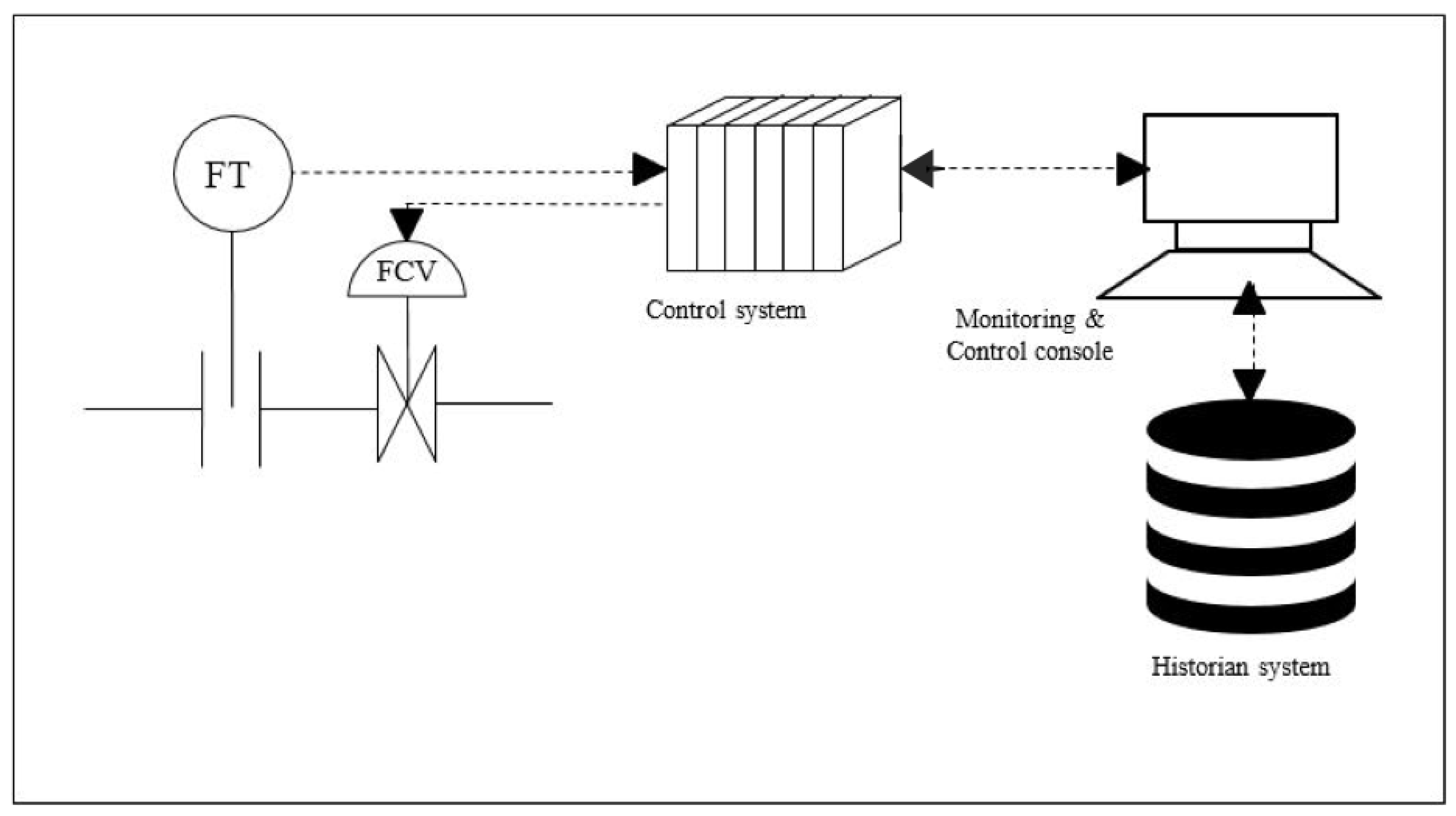
In order to respond to increasing demand for safe and efficient oil and gas plant operation while considering environmental regulations, the subject of “process control” has become increasingly important in recent years [1]. In process control systems, some activities such as supervisory control, data logging and performance monitoring, with their hierarchical relation illustrated in Figure 1, are pursued based on available process variables [2]. These variables include pressure and flow rate of fluids, temperature of flame or materials, liquid level in tanks, and other quantitative items [3]. Some of these variables are measured by sensors, transferred on industrial networks, processed in distributed or central control systems, and monitored in control consoles [4]. Management of the huge amount of process variables of chemical process plants is recently categorized as a “BIG-DATA” concept [5]. Transmission and storage of these variables has considerable cost in many industrial plants, such as oil and gas refineries, and so reduction of these expenses is vital for managers [6].
The main motivation for this research originates from the important issue of “big data management” in large-scale chemical plants. Subjects such as appropriate alarm management, efficient decision-making, and simultaneously handling a large amount of received data in control and monitoring systems imply that an applicable algorithm for reducing the size of stored data is crucial. The presented methodology in this paper is a solution to ignore less important information and just to keep and save the vital data for controlling and monitoring purposes, and also for future studies and analysis. In addition, it should be highlighted that in large-scale chemical plants such as oil and gas refineries, due to high sampling rates and also the large number of field instruments and transmitters, the dedicated costs related to data storage capacity are too high. This issue also persuades field engineers to develop applicable algorithms to decrease the volume of the online and stored data, while not imposing negative effects on normal operational conditions of the plants.
Horch and Isaksson [7] have introduced a method for sampling rate assessment based on the Harris Performance Index [8] for a control system. Adaptive sampling rate has been applied in [9,10] for data size reduction in remote monitoring and control systems. In [11,12,13] real-time and in [14,15] offline data compressing methods have been developed. Another work on this concept can be seen in [6], in which the compression effect on archived data in a control system has been studied. For industrial network performance enhancement, an effective method has been proposed in [16]. Although many other works are in progress on principal component analysis (PCA), which can reduce data size in control systems, the PCA method is not considered in this paper due to its high dependence on data correlation and its inability to reduce data size in the case of non-correlated variables [17]. In addition, the reliability of PCA-based methods depends on process condition stability [17]. Another limitation for this method is transforming the main process values to some new variables which cannot be interpreted by process engineers for process analysis [17]. Furthermore, some of the effects of variable characteristics such as serial correlation of the results of PCA-based methods are still unknown and should be investigated in future research [18]. As previously mentioned, signals and data handling in oil and gas plants are a subset of “Big-Data Management”. According to [5,19,20,21], although the study of chemical plants online and recorded variables can be categorized as a concept of BIG-DATA management, most of the existing methods for handling BIG-DATA are not totally applicable to chemical process controllers due to the following reasons. First, the proposed techniques are mostly appropriate solely for monitoring, and not controlling, purposes. Secondly, the cloud data processing needs outsourcing and hand-overing of data to a third party. In other words, this issue is not a routine task in the chemical industries, especially in oil and gas plants, due to security and safety concerns. Most of the established research noted here has focused only on one aspect of data size reduction in oil and gas plant control and monitoring systems.
The main goal of this article is to develop an applicable algorithm for oil and gas plants to decrease the data size in the control and monitoring system. To this aim, three practical procedures have been introduced in a pilot-scale hydrocarbon refinery to reduce communication, control and storage costs. One method for decreasing the data size and consequently reducing the transmitted data from sensors or input cards to controllers is decreasing the samples at a given time. In this paper, at the first step, selected process variables have been analyzed in the frequency domain for all data gathering periods, by modelling the signals using Fourier transform and fast Fourier transform (FFT) in order to obtain an overall view of frequency components. Next, real signals have been analyzed by the discrete wavelet transform (DWT) method to study frequency component variations in time. We have also executed performance index analysis to verify the obtained results from FFT and DWT analysis by the frequency indirect method in determining sampling rate and data compressing method selection [22]. The performance index analysis technique is more useful for obtaining sampling rate of those process values which cannot be calculated by frequency-domain analysis methods like FFT or DWT. Frequency-domain analysis of process variables is beneficial because for a slow process value, data may be compressed by a simple algorithm and saved in a smaller memory space in comparison with uncompressed data [22]. Frequency analysis results can also be used for control device selection [23]. Some efforts for sampling rate assessment have been made, like the method in [7], by using a performance-index-based method in which an ARMA (auto-regressive moving average) model of a control system was applied. One of the superior aspects of the ARMA model for sampling rate assessment is the prediction of the future behavior of a system [24]. There are also ongoing works to improve the predictive property of the ARMA model [25]. Predictive property is essential for a control system to determine the best sampling rate not only according to the past events, but also to take into account the future conditions. By doing frequency and performance index analysis, a new and useful method for sampling rate selection has been introduced in this paper. In the next step, traffic model of a well-known industrial network (Foundation Fieldbus) has been studied to determine how useful the proposed approach in comparison with other methods is for the reduction of communication traffic in industrial networks, where process variables were studied from a statistical characteristic point of view. One of the most useful statistical criteria is correlation, which shows a relationship between process variables [26]. It may be used for data removing and compressing without information loss. Finally, based on Harris performance index benchmarking [8] and also other technical considerations, negative effects of the proposed methods, for data size reduction on control system performance and safety, have been fully studied. These methods can also be used for other chemical process plants [27], and in this article process variables in a dehydration unit of a gas refinery have been used.
2. Details of the Selected Process Unit
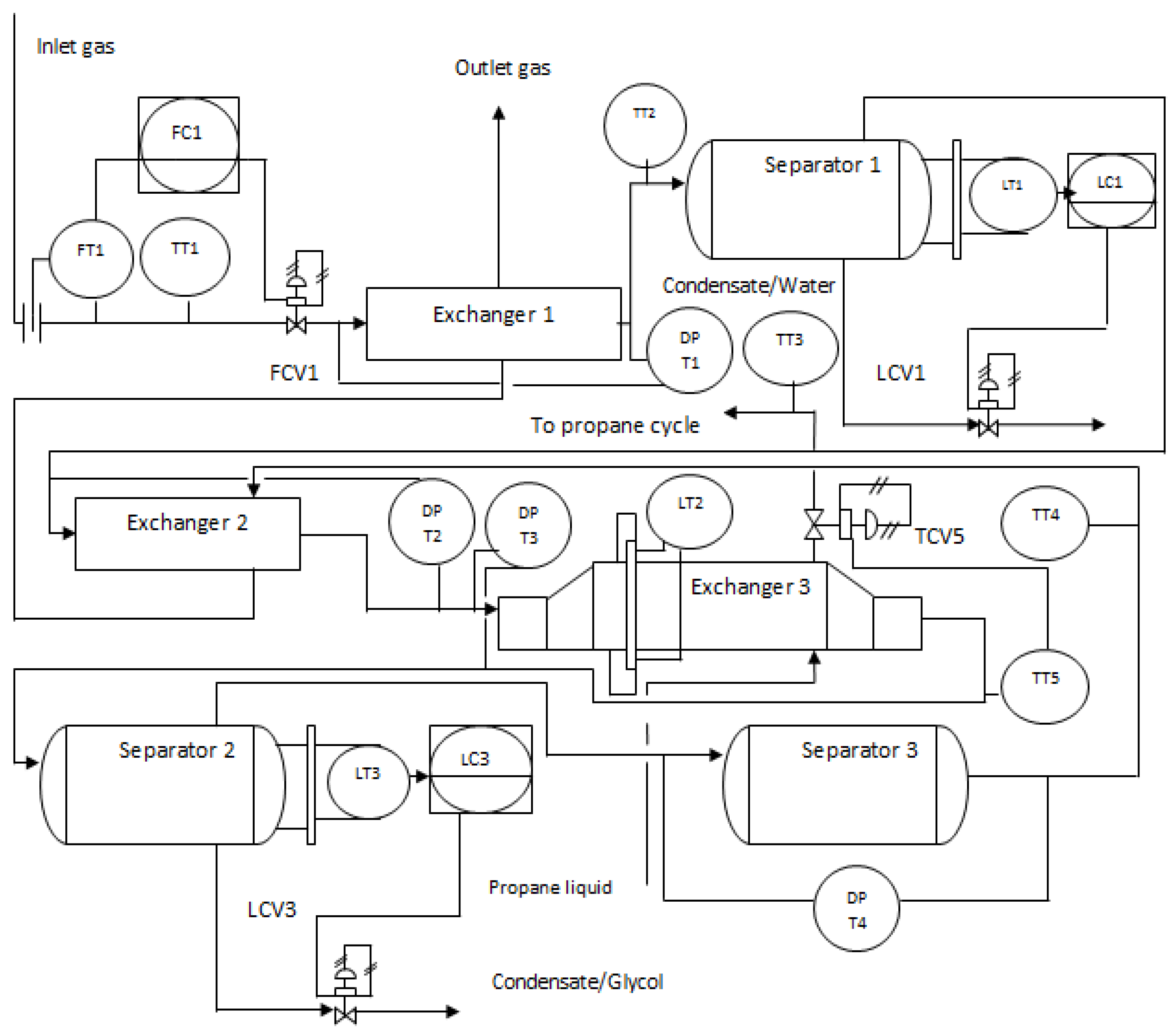
The main function of a dehydration unit, considered in this case study, is to reduce moisture and heavy hydrocarbon components of output gas in a gas refinery. The schematic of the unit and the selected process variables are shown in Figure 2. The applied symbols used in Figure 2 are standard ones recommended by ISA 5.1 1984 [28].
Gas enters Exchanger 1 at a nominal flow rate of 3.4 million cubic meters per day. The temperature of the input gas varies in the range of +50 °C to +70 °C. Exchanger 1 reduces gas temperature to +20 °C. Separator 1 separates condensed liquid from gas. Then, gas enters Exchanger 2 and its temperature decreases to about +5 °C. Finally, it travels to Exchanger 3 and its temperature comes down to about −15 °C. After separating remaining liquids from gas, it returns to Exchanger 2 and Exchanger 1 tube-side for cooling the input gas to the unit, and then leaves the dehydration unit as refinery output gas.
In the normal operation mode of the mentioned unit, the input gas–water component dew point is about +25 °C to +30 °C in summer and +15 °C to +20 °C in winter, and the dew point of output gas is −14 °C in summer and −20 °C in winter. The dew point of heavy hydrocarbon components in the input gas is +40 °C in summer and +30 °C in winter, while for the output gas it is −6 °C in summer and −10 °C in winter.
In the present study, some key process values which have been accessible and have had a main role in the process functionality have been considered.
3. Archived Data Specification
In this paper, the studied data have been taken in an interval of 18 months. The first selected period of time had the greatest changing rate in process values according to the long-term observations and the second batch of data is from moments after an unscheduled shutdown occurrence. The fastest and greatest changes in variables are when the output line pressure is low due to a large flow of gas consumption on the consumer side. The sample rate for data gathering has been set to 5 Hz and we have 27,391 (for normal operation) plus 25,586 (for shutdown condition) samples for each selected process variable. Each sample has been saved as a double floating point variable in the data base [29,30]. Ensemble length and sample intervals are larger than what is recommended in [31].
4. Data Size Reduction Methods
4.1. Frequency Domain and Statistical Analysis
4.1.1. Frequency-Domain Method
Since process variables, which are used and recorded in modern control systems such as programming logic controllers (PLCs), distributed control systems (DCSs) and Fieldbuses, are generally digital [3], discrete Fourier transform (DFT) (fast Fourier transform (FFT)) and discrete wavelet transform (DWT) are appropriate approaches as discrete frequency analysis methods. FFT is utilized for an overall view of frequency components in a signal study time window [32] and the DWT method is a time–frequency analysis and is localized in a time domain [33,34].
In FFT analysis of selected process variables, signal concentrates in 0 Hz and decays rapidly in the near neighborhood of 0 Hz for all process variables. Since most process variables can be estimated by a second order differential equation, whose magnitude decays rapidly after the second pole, it is not necessary to consider process values after the cut-off frequency [1,32]. Table 1 shows a 3 db cut-off frequency for each process value and also a comparison between absolute mean values of a process value (zero frequency component) and a maximum value of FFT analysis.
Figure 3 shows a sample of a FFT curve of a process variable, which looks like a low-pass filter transfer function [35]. It is obvious that the absolute mean value of each process variable is equal to the maximum of frequency component magnitude in FFT analysis. The mean value of a signal is its zero-frequency component magnitude [36]. So, the maximum of frequency component magnitude occurs at zero frequency and this result validates FFT curves.
It can be seen in Table 1 that a 3 db bandwidth of frequency components in FFT analysis is from 0 Hz to frequencies between and . This shows that the shortest period of change in process values is about 5 h.
For further study, the mean value of each process variable has been removed. According to the band-pass property of the frequency-domain pattern of the remaining signal, low and high cut-off frequencies and the peak values in the frequency domain, in comparison with the mean value of process variables, have been stated in percentages in Table 2. In Table 2 it can be seen that 79% of process values have about 0.0001 Hz bandwidth and only DPT3, DPT4 and PT1 have more than 0.0001 Hz bandwidth, which has a small magnitude in comparison with the DC value (under 1%) and hence their bandwidth is not important or influencing [3]. The worst case happens for LT1 which has a 0.0003 Hz cut-off frequency and 7.81% of DC component magnitude as its peak magnitude. For LT1, according to Nyquist rule [32], we need 0.7 h sampling interval as the shortest interval between the samples.
Bandwidth difference between an original signal and a DC-removed signal originates from the fact that bandwidth is obtained from cut-off frequencies according to finding a 3 db frequency drop in comparison with the maximum value of the signal. For signals in which the DC component is dominant, when the DC component is removed, the remaining signal will have a completely different maximum amplitude value and therefore different 3 db frequencies. As a result of FFT analysis of process variables and also based on Nyquist theorem, we found 5 h as the shortest sampling interval for process variables with DC component and 0.7 h for process variables without DC frequency component for change analysis. It is clear that both sampling intervals are too long for typical oil and gas processes to take an action against fluctuation [1].
Generally, FFT analysis for overall frequency-domain analysis is perfect, and other frequency analysis methods cannot give a complete view of the overall properties of a signal in the frequency domain [33]. However, for the detection of frequency components which take place in a short time and cannot be studied in FFT analysis, wavelet analysis may be performed. For wavelet analysis, normally the mother function Daubechies 3 is selected. The reason for this selection is its fast vanishing, orthonormality and also compactly supported property, which shorten calculation time for wavelet transformation beside its relative smoothness [33].
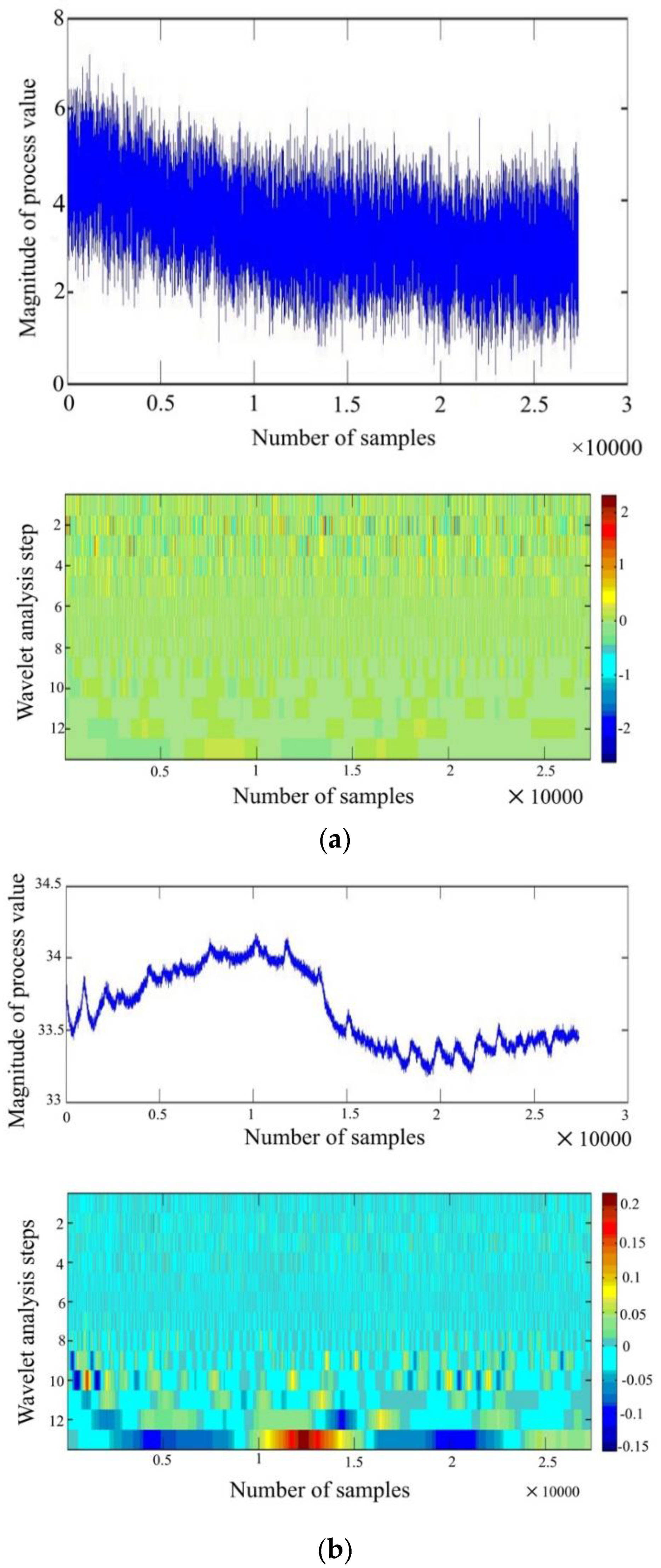
Figure 4a,b shows the time domain and wavelet analysis trend for one of the variables. As it can be seen in Figure 4a,b, the most common background magnitudes (colored) in 2D diagrams are zero. But in TT2, non-zero magnitudes start from step 13 (smallest frequency = 4.8828 × 10⁻⁴ Hz) and continues up to step 9 (0.0078 Hz). In LT2, non-zero magnitudes start from step 13 to 1. It is clear that non-zero magnitude components are observed in some moments, but not for the entire signal existence duration. So, it can be stated that LT2 has instantaneous frequency components in greater frequencies in comparison with TT2.
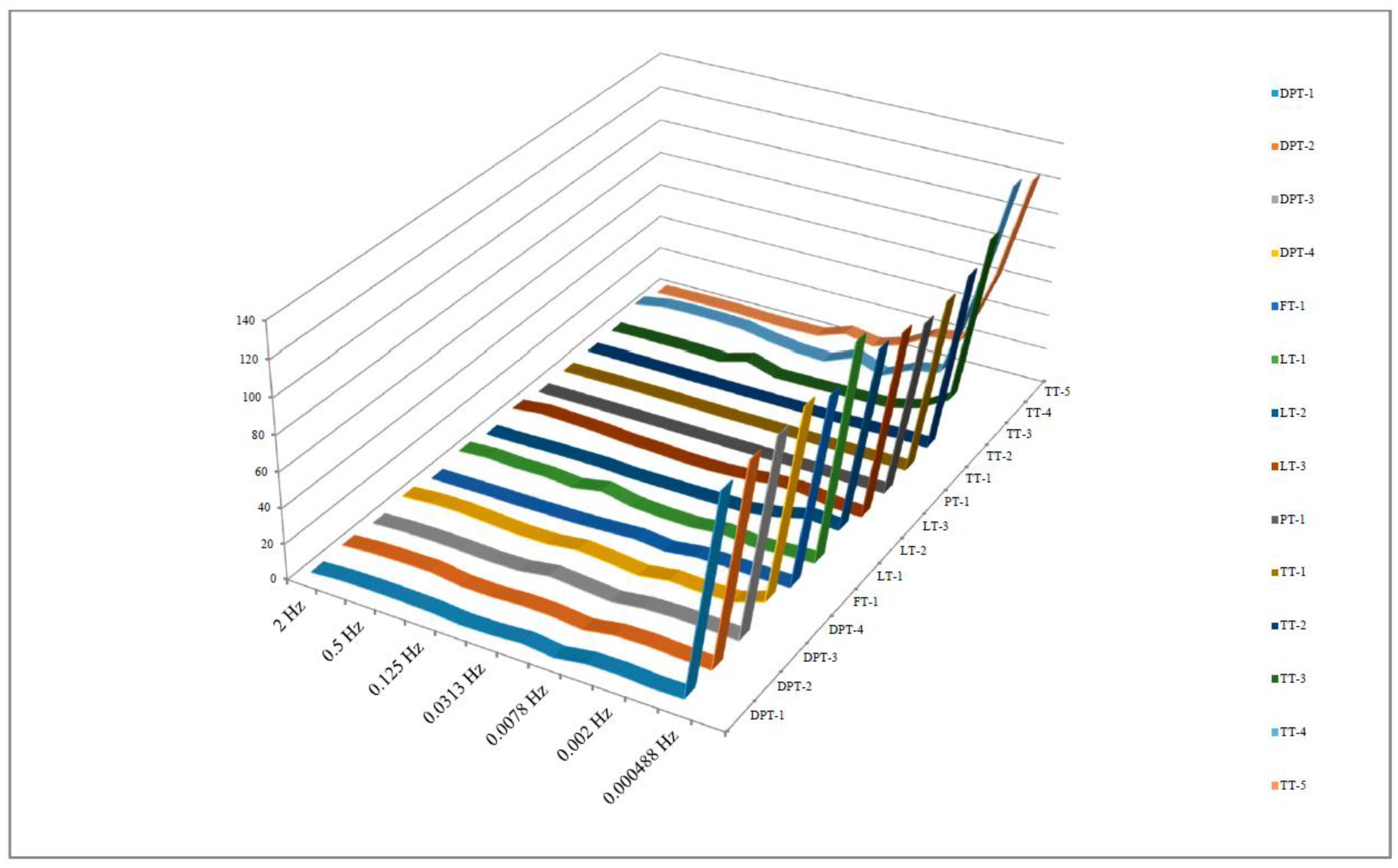
In wavelet output analysis, according to 2D diagrams, no important frequency component is observed at high frequencies except for LT2, LT3, and TT1. In the next step, time-varied frequency components obtained by wavelet analysis for each process value have been studied in detail. In this study, for each step of the process value wavelet analysis, the maximum of absolute value of each step output has been normalized by absolute of the process variable mean value. So, this method shows the ratio of maximum value of a frequency component to the mean value of the process variable (mean value of a process variable is the magnitude of zero frequency component which is generally the dominant frequency in process industries).
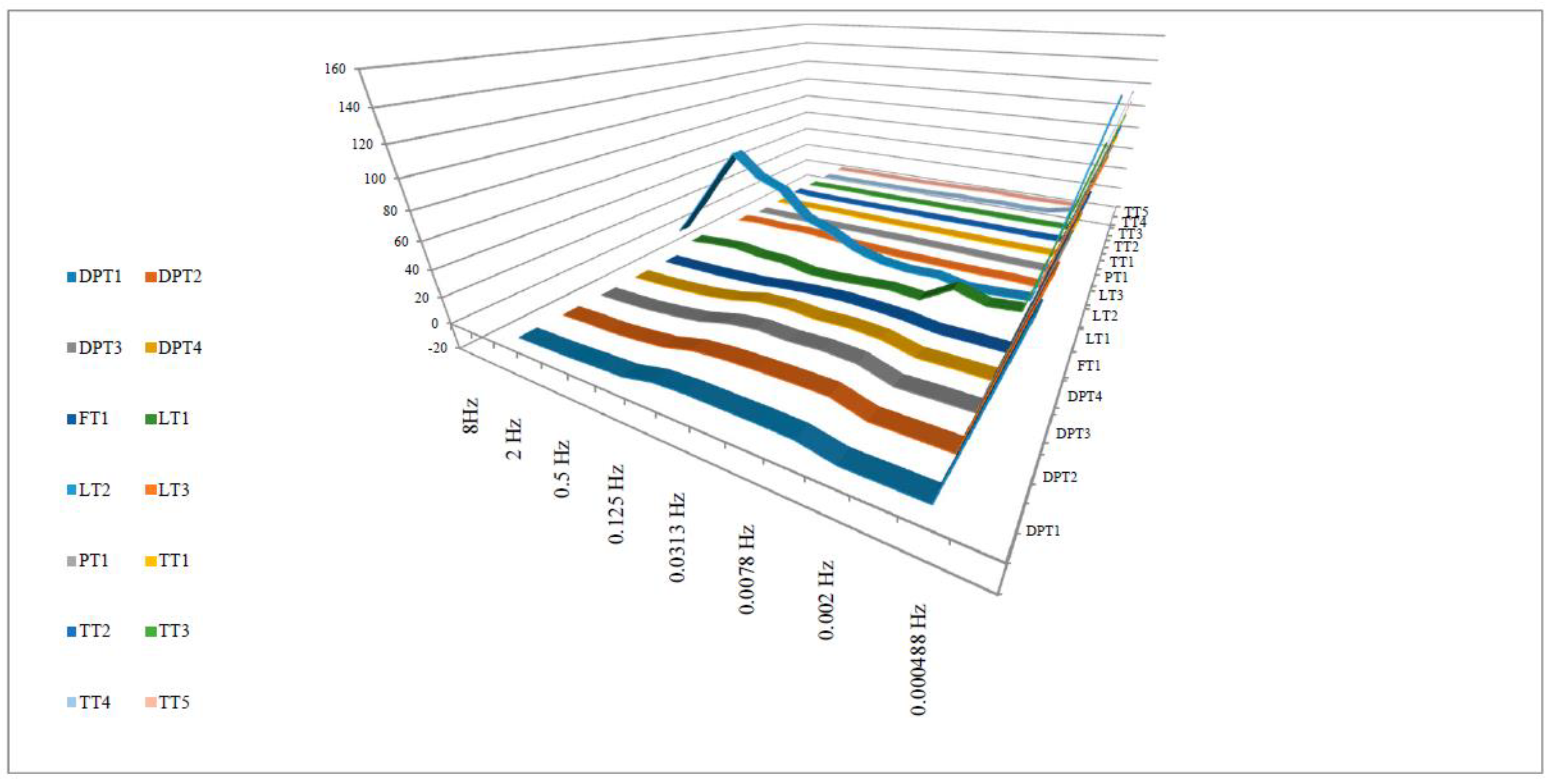
In Figure 5, the ratio of absolute maximum magnitude of process variable time-varied frequency components to absolute of mean value of process variables has been depicted in percentage. It is obvious that, except for LTs, especially for LT2, there are not too many dominant frequency components greater than zero even for the absolute maximum of instantaneous frequency component magnitudes. So, we can claim that there is no valuable frequency component for frequencies greater than zero for process variables.
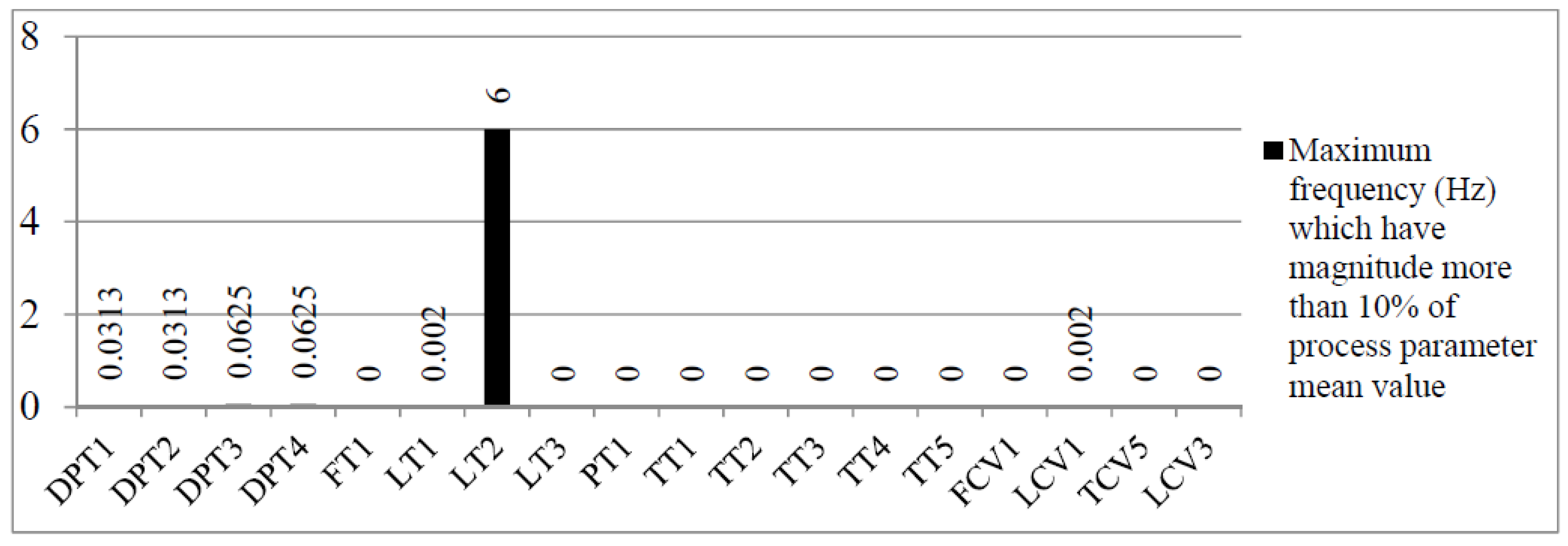
Generally, measurements for control purposes rarely need precision above 10% of the absolute value [3]. For each process variable, the greatest frequency component with its absolute maximum greater than 10% of the process variable mean value is found (as showed in Figure 6), from which the process variable bandwidth, and therefore best sampling rate, are calculated according to Nyquist rule. In this paper, 10% precision for the absolute value of each process variable has been considered.
In Figure 6, the best sampling rate can be obtained by doubling the frequency, which is written above the bars, for related process variables. These sampling rates are slower in comparison with the recommended refresh rate for process variables in the American Petroleum Standard API RP 554 [37] for a proportional integral derivative (PID) loop controller, which is 50 Hz.
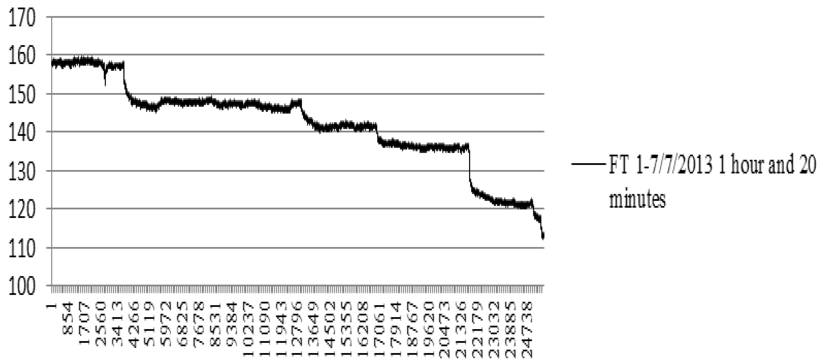
To validate the obtained results, data for an unscheduled plant shutdown have been studied. As it can be seen in Figure 7 and Figure 8, for FT1, which measures the main process variable that passes through the whole unit, unscheduled plant shutdown data was changing much slower in comparison with normal operation mode. FFT analysis for unscheduled shutdown trends shows that 3 db bandwidth for all process values is about . In addition, in Figure 9 it is obvious that from wavelet analysis results for the fastest process variable (LT1), the greatest amplitude of frequency components takes place at a frequency of 1 Hz. Magnitude of this frequency component, for ordinary operation, is about 80% and for unscheduled shutdown is about 10% of the DC frequency component value.
By performing FFT analysis, it can be observed that the frequency bandwidth of process values in both normal operation and unscheduled shutdown cases is about . However, by applying wavelet frequency–time analysis for finding transient events, it can be said that the unscheduled shutdown case has no process-variable transient changing (substantial transient frequency component greater than 0 Hz component) faster than the normal operation case.
For a more precise study of the process variables in both the worst case of normal operation and also occurrence of an unscheduled shutdown, an analytical support for the obtained results by applying direct signal processing over the measured process variables and also proof for frequency component analysis of signals have been presented. In the dehydration unit, the main process variable is the flow rate of natural gas. So, this variable (FT1) has been selected to be modeled and also to provide mathematical and theoretical calculations to find an exact and closed form of the frequency-domain formula. In the normal operation case, the mathematical model of FT1 signal is a superposition of two types of Poisson narrow triangular pulse trains, which are different in height as depicted in Figure 7. For the unscheduled shutdown case, FT1 is a superposition of step functions, as can be seen in Figure 8. For the first case (worst case of normal operation), the narrow triangular-pulses happening distribution in the time domain is assumed as a Poisson distribution, because it satisfies three conditions of Poisson processes stated by Chung and AitSahila [38]. Due to the Oppenheim, Willsky and Nawab statement [32], for the Poisson triangular pulse train it can be said that it is the result of the convolution of a triangle pulse and a Poisson impulse train in the time domain. The frequency-domain equation of a triangle pulse is [32]:
And frequency-domain equation for Poisson impulse train is [39]:
It is obvious that the convolution in time domain equals multiplying the frequency domain [32]. So, the frequency-domain definition of the Poisson triangular pulse train would be
By assuming T to be small enough, sin c2 term in Equation (3) will be very small and Equation (3) becomes
which shows 0 Hz property of signal and corresponds with results of frequency analysis from FFT and DWT of signals.
For an unscheduled shutdown signal, it can be seen that in the selected time window, the signal is the superposition of step functions as shown in Equation (5),
while
Hence, in the frequency domain we have [32]:
By taking into account condition (6), the term in parentheses will be a positive value k and the result reduces to Equation (8):
From Equation (8), it is clear that the unscheduled shutdown signals also have a dominant 0 Hz component and behave as a DC signal. This result corresponds with results of frequency analysis from the FFT and DWT of the signal.
4.1.2. Adaptive Sampling Rate Method Investigation
In this method, the sampling rate of process variables varies based on the rate of their changes (signal frequency-domain property) [10].
In existing control networks adopted for oil and gas plants, such as Foundation Fieldbus, measurements and commands for controlling purpose are categorized as scheduled transmissions, for which their transmission interval cannot be changed [40]. In addition, in control networks in other type of plants, besides sending measurements and receiving commands from remote supervisors in an adaptive sampling rate, control and monitoring systems include local main controllers which do not use an adaptive sampling rate. This policy is generally being followed to increase the total reliability of the plant [10].
It shows that the adaptive sampling rate has not been assessed as a reliable solution for control purposes in critical plants.
4.1.3. Performance Index Based Analysis
Based on performance index for control loops introduced by Harris [8], an approach to obtaining the almost-optimal sampling rate for controlling purposes has been developed by Alexander Horch and Alf J. Isaksson [7]. In this article, the mentioned approach for performance-index calculation has been used in a different way, in which its aim is finding the best sampling rate of control and also data storage systems of process variables. To find the best sampling rate using a performance index criterion, first, the fastest available sampling rate in a well-tuned controlling system can be used and the performance index will be calculated. If the selected sampling rate is greater than the needed value, the process variable time series present noisy behavior. So, the performance index becomes less than one due to oversampling and also taking many samples during the system time delay [6]. In the next step, samples will be picked up at a lower frequency, from the original ensemble of data. So, the process variable time series demonstrate more predictability, and the performance index will go up. By iterating the previous steps, and in each step picking up samples from the original sample series at a lower frequency, the performance index will increase. The sampling period which causes the performance index to become equal to one will be selected as the appropriate sampling rate. For applying the proposed method over the selected unit, in the first step an auto-regressive moving average (ARMA) model for the control loop in 1/80 of the basic sample rate (16 sec interval) has been considered. For more details on ARMA structure refer to [41]. ARMA model parameters for the subsystems studied in this paper are summarized in Table 3.
The performance index for 1/80 of the basic sample rate is equal to 2.06. The performance indexes for other data-saving sampling rates have been summarized in Figure 10. As it has been depicted, by decreasing the sample pick-up interval, performance index decreases, and for a specific interval it is equal to 1. For each control system, it is not possible to have intervals greater than the delay size between input and output. For LT2, due to controller sampling rate limitation and its wide frequency band, frequency components more than the basic sampling rate frequency cannot be tracked. As a result, curves after sampling rate frequency would be estimated by linear extrapolation.
By comparison of sampling intervals obtained in Figure 10 for selected process variables from the performance index analysis with those obtained from wavelet analysis, it can be deduced that performance index results have a smaller sampling period (greater sampling rate) than the obtained results from wavelet analysis. Hence, they can capture more precisely the fast phenomena details and changes. The obtained results have been summarized in Table 4.
Finally, although in this paper applicability of the proposed method has been presented for both normal operation and unscheduled shutdown cases, it should be reminded that during shutdown or startup condition all systems are in a manual state and, in fact, there is no need to apply the calculated sample rates to the control systems.
4.1.4. Combination of Frequency and Statistical Analysis Methods
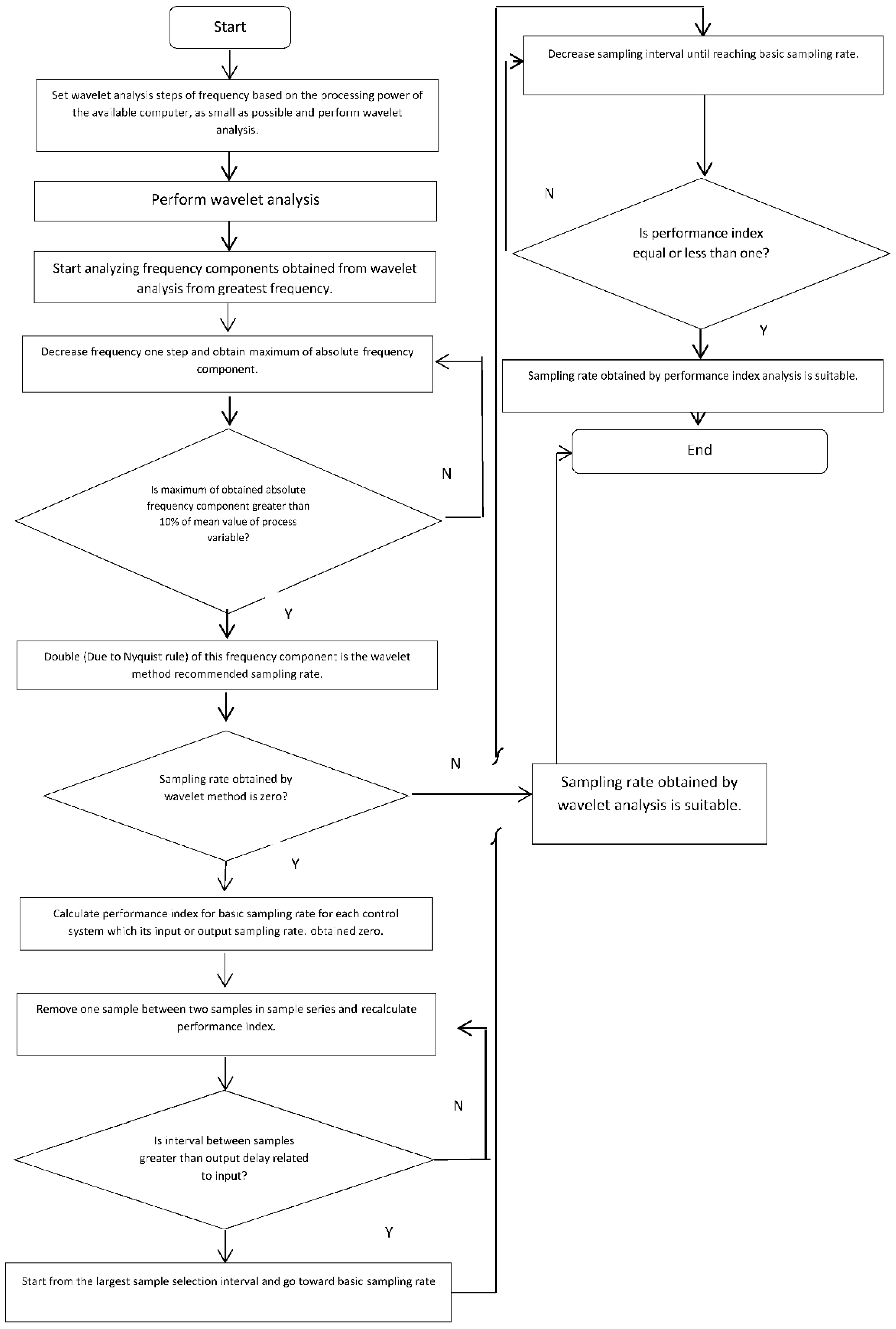
By combining both wavelet and performance index methods, the flowchart for the developed algorithm to find a sampling interval for the process variables is presented in Figure 11.
Moreover, it should be noted that sampling rate plays a vital role in modern process control systems. In other words, these systems are completely digital, and what connects real analog process values to the digital world is sampling rate selection. An illustration of the sampling mechanism and a comparison between conventional and proposed sampling-rate determination methods are shown in Figure 12.
To find the best sampling rate in oil and gas plant process control and monitoring systems, sampling rates obtained by conventional methods are compared with the sampling rates using the proposed method as shown in Table 4.
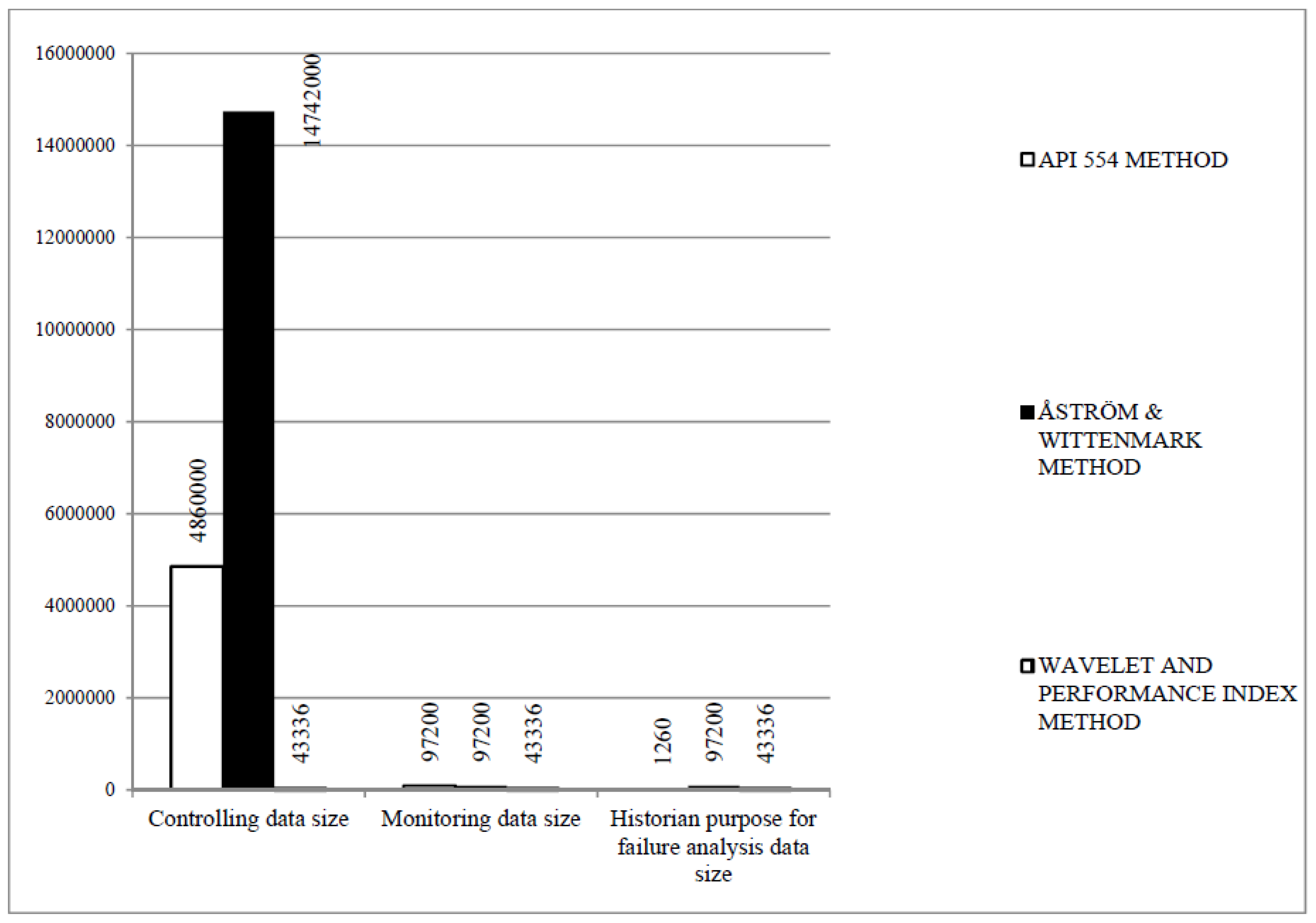
Figure 13 illustrates the size of data which were generated in 1.5 h from sampling rates obtained by using the proposed method in this paper for all process values in a gas refinery dehydration unit, compared to the conventional methods mentioned in Table 4. Numerical interpretation of Figure 13 can be seen in Table 5. It should be noted that for the outputs of the control system, such as control valve commands, the sampling rate of the input of the control loop may be used, because the output frequency spectrum of a control loop is the multiplication of the input spectrum and control loop transfer function spectrum. The output frequency spectrum is like a low-pass filter [1]. As it can be seen in Figure 13, for controlling purposes, the sampling interval calculated by the presented method would reduce the data communication traffic and data processing load of the controller by more than 99.11% in comparison with the API 554 method. For monitoring purposes, the presented technique will also reduce data size by 55.42% in comparison with the API 554 method. However, for historian purposes, the introduced method increases the size of data approximately 33.4 times. In comparison with the Åström and Wittenmark method [1], in controlling purposes about 99.71% and for both monitoring and historian purposes about 55.42% reduction in data size was observed. The reason for increasing data in comparison with the API 554 method for historian purposes is because of the disability of the API 554 method in historian purposes, to show the process dynamics. According to the API 554 standard, for the studies which may be done during the 30 days after data recording, the recorded data may be used for process behavior and failure analysis. So, it should consist of process dynamics. Among all the mentioned methods, only the presented technique can show process dynamics in historian purposes properly. So, it is not a drawback if the size of the data collected by this method is greater than other approaches for historian purposes.
For verification of previous studies, data gathered in an unscheduled shutdown have been studied. The results show that for TT2, LT1, LT2 and DPT1 frequency-band widths are almost zero for all cases. This observation shows slower changes for an unscheduled shutdown case, compared to the normal operation worst-case signals. The obtained results verify the theoretical frequency-domain analysis of process variables and the slow rate of changes, presented in Section 4.1.1.
4.2. Traffic Model Analysis
Industrial networks can be modelled as a queuing system. This is possible because published packets on the network can be assumed to be arriving customers, and the length of a packet as the serving time of the server.
Foundation Fieldbus as an industrial network sample can be defined in Kendall’s notation as a D/D/1 traffic model. D stands for Deterministic (Figure 14) [40,42]. As a result, the time of packet transmission starting and its duration are known and cannot be changed.
Whereas a macrocycle is the least common multiple of the entire loop times on a given link [43], it will be possible to take the length of a macrocycle for the control system studied in this paper as 500 s. For existing fieldbus systems, such as the Delta-V system, we have a maximum 5 s length for the macrocycle [44] and this value could be revised according to the results of this paper. This extension of the macrocycle time is possible because for variables DPT1, DPT2, DPT3, DPT4, FT1, LT1, LT3, PT1, TT1, TT2, TT3, TT4 and TT5, the publishing period can be 500 s instead of 5 s. Using the proposed macrocycle in the presented manuscript and also the introduced methods in [16] for data obtaining after applying the sample-rate changing method in Section 4.1.4, it is possible to make a larger capacity for the Foundation Fieldbus network. For example, for the studied dehydration unit, saving about 82% of the occupied communication time is feasible. It should be noted that the time-saving calculated for the Foundation Fieldbus system is in comparison to the traffic for data after applying the enhanced sampling rate, not in comparison with the API 554 method sampling-rate selection. As a result, installing more transmitters on a Fieldbus network segment instead of 32 devices, which is the maximum capacity for a H1 segment [45], would be possible.
4.3. Correlation Analysis
In this section, a correlation analysis of process variables has been presented. From linear correlation, we cannot judge non-linear correlation. So, as a complementary test of this method, a visual check of scatter diagrams of each pair of process values, which have correlation factors between +0.8 and −0.8, has been performed and no meaningful correlation in that range has been detected. In this study, correlation analysis between process variables in two cases (normal operation and unscheduled shutdown) has been done.
These correlations and process-variables coupling in an oil and gas plant are often due to the laws of fluid mechanics which relate them to each other. By the aspect of the control system which has been considered in this paper, there is good linear correlation for DPT1, DPT2, DPT3, DPT4, PT1 and FT1 and also between TT3 and TT5 in a normal operation case. Moreover, there is a linear correlation for DPT1, DPT2, DPT3, DPT4, PT1 and FT1 and also for TT3, TT4 and TT5 in an unscheduled shutdown case. As a result, the removal of 4 process variables in a normal operation case and 5 process variables in an unscheduled shutdown case is acceptable.
Using the presented method in this section (for normal operation case), 55.56% (and if its association with changing sampling-rate method is used, 99.19%) of the data resources in the control system can be saved in comparison with the API 554 technique. For an unscheduled shutdown case, even removing redundant data is more effective to reduce data size, because instead of 5 variables, 6 variables are removed.
The results of using only this method and also associated with other methods for data monitoring and storage, and traffic (networking) systems, can be seen in Table 6.
5. Effect of Proposed Data Size Reduction Methods on Control System Performance and Plant Safety
For the implementation of data size reduction methods in industrial oil and gas plants introduced in the previous sections, it is essential to determine that the proposed techniques have no negative effect on control system performance and plant safety. Related to “process safety and control” concerns, three reasons can be mentioned:
- (A)
- It should be ensured that any important change in the selected process variables is not missed, which enables the control/safety system to take an on-time and accurate reaction as a response. Hopefully, by applying a time–frequency analysis method (DWT method), finding drastic changes in the process variables is possible. As a result, by choosing a fast enough sampling rate, based on the presented methodology and according to time–frequency analysis, a suitable scheme can be designed to guarantee not to miss important changes in the selected process variables.
- (B)
- Another issue which may cause the missing of important changes in the process variables is the high volume of calculations between two consecutive sampling times. To prove this concept, the Harris performance index is a reliable benchmarking tool [8]. Two essential factors that affect the Harris performance index are sampling rate and controller dead-time [7]. So, for each method, the effects on these two factors are evaluated to find out whether they have any side effects on the control system performance.
5.1. Sampling Rate Changing Method
Because sampling rate is fixed, it needs minimum processing power and it cannot cause significant delay due to increasing processing time. So, this method has no side effect on control system performance.
5.2. Traffic Enhancement Method
From a delay point of view, there exists no difference compared to the Foundation Fieldbus network, which is widely utilized in oil and gas plants. So, it has no negative effect on control system performance.
5.3. Correlation Analysis Method
By selecting the fastest sampling rate among linear correlated process variables, no negative effect on sampling rate of process variables will appear.
For delay analysis in this method, it can be stated that one real analog input is used as a main process variable. Then, by utilizing a linear equation like Equation (9), other variables which have linear correlation with the selected one are calculated.
In industrial PLCs which are known as the main controllers in oil and gas plants, the program runs in a scanning manner. Each duration of the program running from start to end is called a scan time. Scan time depends on the number and types of instructions in the program, the interrupts and their duration, and the CPU type. Its typical duration can be from 5 ms to 20 ms or even more [46]. So, for investigating the delay effect of analog input by removing by correlation analysis method, time of multiplication and summation together in Equation (9) should be stated as a percentage of a typical scan time. This concept has been studied on a S7-400 CPU in a SIEMENS SIMATIC PLC system [47]. Floating-point math instructions have 0.3 μs duration, which is 0.006% of total scan time. This fact shows that the correlation-based method of data size reduction has no considerable effect on control system delay.
- (C)
- Finally, there are many safety associated systems/equipment generally embedded in chemical plants, such as emergency shut down (ESD), safety and relief valves, which ensure a safe operation even if failures occur in the regular “control and monitoring” system.
Thus, it can be concluded that the method presented in this paper to reduce the data size in typical oil and gas plants does not have a negative impact on the total performance of the control system and also plant safety.
6. Conclusions
In this paper, several process variables in a gas refinery dehydration unit in the frequency domain and also statistical, traffic and correlation points of view have been analyzed to find applicable methods of data size reduction. To check the general characteristics of the presented method, a normal operation worst-case and an unscheduled shutdown case have been studied. Adaptive sampling rate in oil and gas plants has been assessed and recognized as an improper method due to lack of reliability in industrial networks and also slow rate of change across many process variables.
In comparison with common techniques, by applying the introduced method, data size reduced to more than 99% for controlling purposes and more than 55% for monitoring objectives. In addition, there was no data size reduction for historian purposes, compared to the API 554 method. Using Harris performance-index benchmarking, it has been demonstrated that the data size reduction methods proposed in this paper have no negative effect on the control system performance and plant safety. Moreover, by applying the proposed methods, cost and size of the control system storage facilities, network hardware, and also input signal devices can be dramatically reduced, without significant data loss. Furthermore, as a future research plan, non-linear correlation analysis of the process variables can be considered to increase the efficiency of the presented methodology.
Author Contributions
Conceptualization, all the authors.; methodology, R.A. and F.H.; software, R.A.; validation, R.A. and F.H.; formal analysis, R.A. and F.H.; investigation, all the authors; data curation, R.A., F.H. and C.M.R.M.; writing—original draft preparation, R.A.; writing—review and editing, F.H., C.M.R.M. and A.E.; visualization, all the authors; supervision, C.M.R.M. and A.E.; project administration, A.E.; All authors have read and agreed to the published version of the manuscript.
Funding
This research received no external funding.
Acknowledgments
The first author would like to appreciate for Sarkhoon and Qeshm Gas Treating Company supports, especially H. Saiiar and M. Jafari from Sarkhoon Gas refinery.
Conflicts of Interest
The authors declare no conflict of interest.
References
- Seborg, D.; Edgar, T.; Mellichamp, D. Process Dynamics and Control; Wiley: New York, NY, USA, 2004. [Google Scholar]
- Couper, J.R.; Penney, W.R.; Fair, J.R. Chemical Process Equipment Revised 2E: Selection and Design; Gulf Professional Publishing: Houston, TX, USA, 2009. [Google Scholar]
- McMillan, G.K.; Considine, D.M. Process/Industrial Instruments and Controls Handbook; McGraw Hill: New York, NY, USA, 1999. [Google Scholar]
- Park, J.; Mackay, S. Practical Data Acquisition for Instrumentation and Control Systems; Newnes, Elsevier, IDC Technologies: Perth, Australia, 2003. [Google Scholar]
- Chiang, L.; Lu, B.; Castillo, I. Big Data analytics in chemical engineering. Annu. Rev. Chem. Biomol. Eng. 2017, 8, 63–85. [Google Scholar] [CrossRef] [PubMed]
- Thornhill, N.F.; Shoukat Choudhury, M.; Shah, S.L. The impact of compression on data-driven process analyses. J. Process Control 2004, 14, 389–398. [Google Scholar] [CrossRef] [Green Version]
- Horch, A.; Isaksson, A.J. Assessment of the sampling rate in control systems. Control Eng. Pract. 2001, 9, 533–544. [Google Scholar] [CrossRef]
- Desborough, L.; Harris, T. Performance assessment measures for univariate feedback control. Can. J. Chem. Eng. 1992, 70, 1186–1197. [Google Scholar] [CrossRef]
- Jain, A.; Chang, E.Y. Adaptive sampling for sensor networks. In Proceedings of the 1st International Workshop on Data Management for Sensor Networks: In Conjunction with VLDB, Chicago, IL, USA, 27 June–2 July 2004; pp. 10–16. [Google Scholar]
- Zheng, L.; Chow, M.-Y. Adaptive multiple sampling rate scheduling of real-time networked supervisory control system-part I. In Proceedings of the IECON 2006—32nd Annual Conference on IEEE Industrial Electronics, Paris, France, 6–10 November 2006. [Google Scholar]
- Mah, R.; Tamhane, A.; Tung, S.; Patel, A. Process trending with piecewise linear smoothing. Comput. Chem. Eng. 1995, 19, 129–137. [Google Scholar] [CrossRef]
- Watson, M.J.; Liakopoulos, A.; Brzakovic, D.; Georgakis, C. A practical assessment of process data compression techniques. Ind. Eng. Chem. Res. 1998, 37, 267–274. [Google Scholar] [CrossRef]
- Hale, J.C.; Sellars, H.L. Historical data recording for process computers. Chem. Eng. Prog. 1981, 77, 11. [Google Scholar]
- Donoho, D.L.; Vetterli, M.; DeVore, R.A.; Daubechies, I. Data compression and harmonic analysis. IEEE Trans. Inf. Theory 1998, 44, 2435–2476. [Google Scholar] [CrossRef] [Green Version]
- Nesic, Z.; Davies, M.; Dumont, G. Paper machine data analysis and compression using wavelets. Tappi J. 1997, 80, 191–204. [Google Scholar]
- Hodson, R. Optimizing Fieldbus Link Schedules Makes a Difference! ISA EXPO 2005, 2005, 1711. [Google Scholar]
- Bezergianni, S.; Kalogianni, A. Application of principal component analysis for monitoring and disturbance detection of a hydrotreating process. Ind. Eng. Chem. Res. 2008, 47, 6972–6982. [Google Scholar] [CrossRef]
- AlGhazzawi, A.; Lennox, B. Monitoring a complex refining process using multivariate statistics. Control Eng. Pract. 2008, 16, 294–307. [Google Scholar] [CrossRef] [Green Version]
- Ur Rehman, M.H.; Liew, C.S.; Abbas, A.; Jayaraman, P.P.; Wah, T.Y.; Khan, S.U. Big data reduction methods: A survey. Data Sci. Eng. 2016, 1, 265–284. [Google Scholar] [CrossRef] [Green Version]
- Khan, A.R.; Schioler, H.; Kulahci, M.; Knudsen, T. Big data analytics for industrial process control. In Proceedings of the 2017 22nd IEEE International Conference on Emerging Technologies and Factory Automation (ETFA), Limassol, Cyprus, 12–15 September 2017; pp. 1–8. [Google Scholar]
- Moyne, J.; Iskandar, J. Big data analytics for smart manufacturing: Case studies in semiconductor manufacturing. Processes 2017, 5, 39. [Google Scholar] [CrossRef] [Green Version]
- Salomon, D. Data Compression: The Complete Reference; Springer: Berlin/Heidelberg, Germany, 2004. [Google Scholar]
- Lipták, B.G. Instrument Engineers’Handbook, Volume Two: Process Control and Optimization; CRC Press: Boca Raton, FL, USA, 2005; Volume 2. [Google Scholar]
- Baptista, M.; Sankararaman, S.; de Medeiros, I.P.; Nascimento, C., Jr.; Prendinger, H.; Henriques, E.M. Forecasting fault events for predictive maintenance using data-driven techniques and ARMA modeling. Comput. Ind. Eng. 2018, 115, 41–53. [Google Scholar] [CrossRef]
- Bao, Y. A general result on the estimation bias of ARMA models. J. Stat. Plan. Inference 2018, 197, 107–125. [Google Scholar] [CrossRef]
- Von Storch, H.; Zwiers, F.W. Statistical Analysis in Climate Research; Cambridge University Press: Cambridge, UK, 2001. [Google Scholar]
- Erwin, D.L. Industrial Chemical Process Design; McGraw Hill Professional: Pennsylvania Plaza, NY, USA, 2002. [Google Scholar]
- Norma, I. 5.1 Instrumentation Symbols and Identification; ANSI/ISA: Research Triangle Park, NC, USA, 1992. [Google Scholar]
- Markstein, P.W. The New IEEE-754 Standard for Floating Point Arithmetic. In Numerical Validation in Current Hardware Architectures; Springer-Verlag Berlin and Heidelberg GmbH & Co.: Berlin/Heidelberg, Germany, 2008. [Google Scholar]
- Citect Facilities 7.10 Service Pack 4- Release Notes. 2011. Available online: https://docplayer.net/1303759-Citectscada-7-10-release-notes-for-service-pack-4.html (accessed on 30 September 2019).
- Thornhill, N.; Oettinger, M.; Fedenczuk, P. Refinery-wide control loop performance assessment. J. Process Control 1999, 9, 109–124. [Google Scholar] [CrossRef] [Green Version]
- Oppenheim, A.V.; Willsky, A.S.; Nawab, S.H. Signals and Systems; Prentice-Hall Englewood Cliffs: Upper Saddle River, NJ, USA, 1983; Volume 2. [Google Scholar]
- Daubechies, I. Ten Lectures on Wavelets; SIAM: Philadelphia, PA, USA, 1992; Volume 61. [Google Scholar]
- Percival, D.B.; Walden, A.T. Wavelet Methods for Time Series Analysis (Cambridge Series in Statistical and Probabilistic Mathematics); Cambridge University Press: Cambridge, UK, 2000. [Google Scholar]
- Carlson, A.B.; Crilly, P.; Rutledge, J. Communication Systems: An Introduction to Signals and Noise in Electrical Communication; McGraw Hill Professional: Pennsylvania Plaza, NY, USA, 1986. [Google Scholar]
- Bissell, C.C.; Chapman, D. Digital Signal Transmission; Cambridge University Press: Cambridge, UK, 1992. [Google Scholar]
- API RP 554: Process Instrumentation and Control; American Petroleum Institue: Washington, DC, USA, 1995.
- Chung, K.L.; AitSahlia, F. Elementary Probability Theory: With Stochastic Processes and an Introduction to Mathematical Finance (Undergraduate Texts in Mathematics); Springer-Verlag: New York, NY, USA, 2003. [Google Scholar]
- Beutler, F.J.; Leneman, O.A. The spectral analysis of impulse processes. Inf. Control 1968, 12, 236–258. [Google Scholar] [CrossRef] [Green Version]
- Glanzer, D. Technical Overview: Foundation Fieldbus, FD-043 Revision 2.0; Fieldbus Foundation: Austin, TX, USA, 1998. [Google Scholar]
- Brockwell, P.J.; Davis, R.A. Time Series: Theory and Methods; Springer Science & Business Media: Berlin/Heidelberg, Germany, 2013. [Google Scholar]
- Sigua, R.G. Fundamentals of Traffic Engineering; UP Press: Metro Manila, Philippines, 2008. [Google Scholar]
- Corporation, N.I. Foundation Fieldbus Overview; National Instruments: Austin, TX, USA, 2011; Volume 370729C-01. [Google Scholar]
- Services, F.-R.E. Course 7032 Foundation Fieldbus Systems & Devices. 2000. Available online: http://www.emersonprocesscourseadvisor.eu (accessed on 30 September 2019).
- Mackay, S.; Wright, E.; Park, J. Practical Data Communications for Instrumentation and Control; Newnes, Elsevier, IDC Technologies: Perth, Australia, 2003. [Google Scholar]
- Yadav, D.; Singh, A.K. Microcontroller: Features and Applications; New Age International: New Delhi, India, 2004. [Google Scholar]
- SIMATIC. Auto Mation System S7-400 CPU Specification. 2008, Volume A5E00267840-03. Available online: http://www.tk-siemens.com/upload/PDF/tk-siemense.com-S7400.pdf (accessed on 30 September 2019).
Figure 1.
A schematic of hierarchical connections of control, monitoring and historian systems.

Figure 2.
Process flow diagram (PFD) of a typical dehydration unit in a gas refinery plant. (DPT, PT, FT, TT, LT stand for differential pressure, pressure, flow, temperature, and level transmitters, FC and LC stand for flow and level controllers, and FCV and LCV stand for flow and level control valves).

Figure 3.
Fast Fourier transform (FFT) curve of DPT1 as a sample of process variables FFT curves.
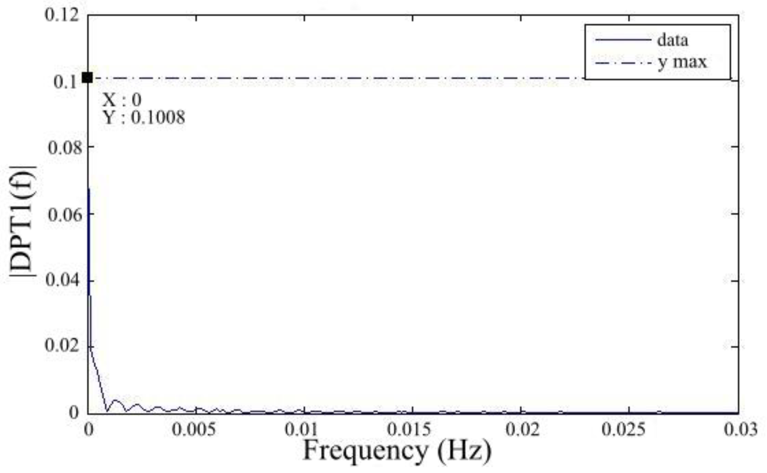
Figure 4.
Time domain and steps of discrete wavelet transform trends for (a) LT2 (b) TT2.

Figure 5.
Absolute maximum magnitude of time-varied frequency components in wavelet analysis as a percentage of absolute mean of process values in normal operation for the worst case scenario.
Figure 5.
Absolute maximum magnitude of time-varied frequency components in wavelet analysis as a percentage of absolute mean of process values in normal operation for the worst case scenario.

Figure 6.
Maximum frequency which has components more than 10% of the process variable mean value.

Figure 7.
Time domain trend for FT1 in normal operation, worst case scenario.
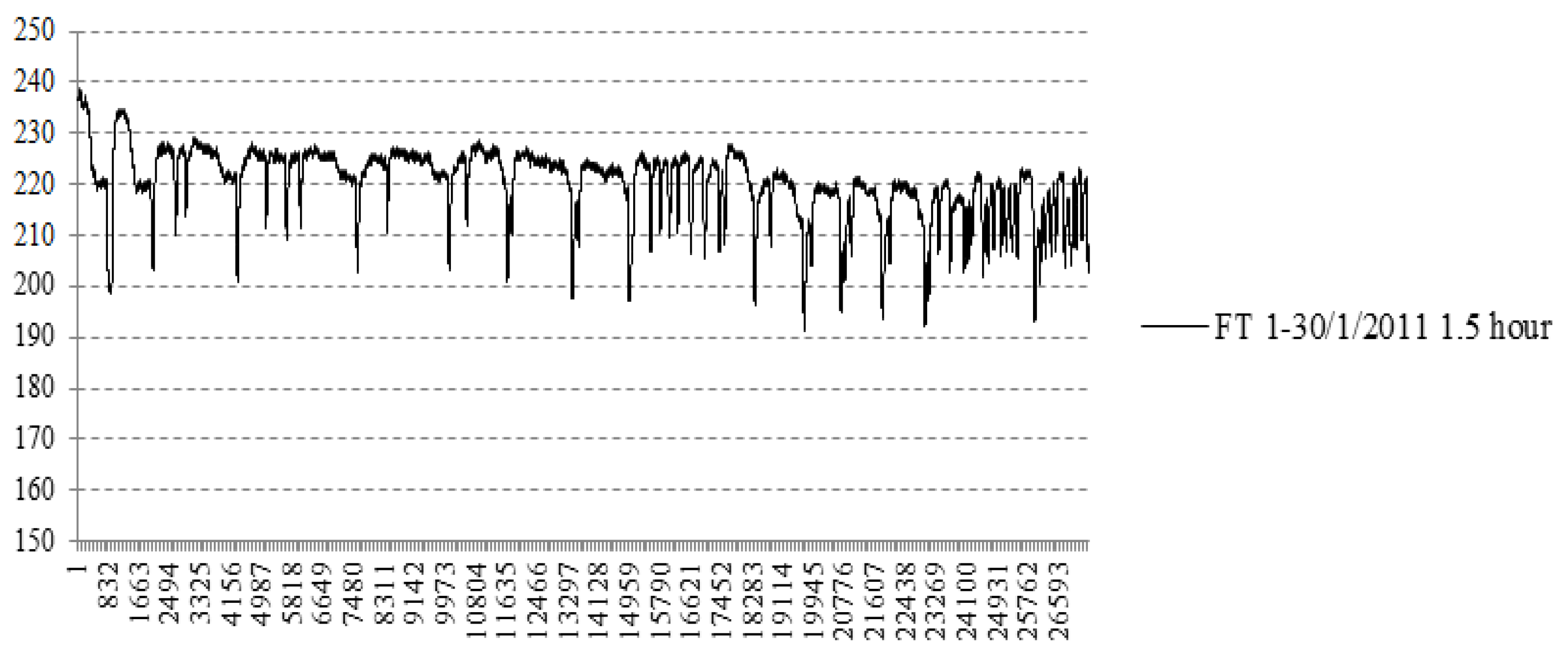
Figure 8.
Time domain trend for FT1 in unscheduled shutdown case.

Figure 9.
Absolute maximum magnitude of time-varied frequency components in wavelet analysis as a percentage of absolute mean of process value in an unscheduled shutdown case.
Figure 9.
Absolute maximum magnitude of time-varied frequency components in wavelet analysis as a percentage of absolute mean of process value in an unscheduled shutdown case.

Figure 10.
Variations in performance index due to sample pick-up interval change in four control blocks.
Figure 10.
Variations in performance index due to sample pick-up interval change in four control blocks.
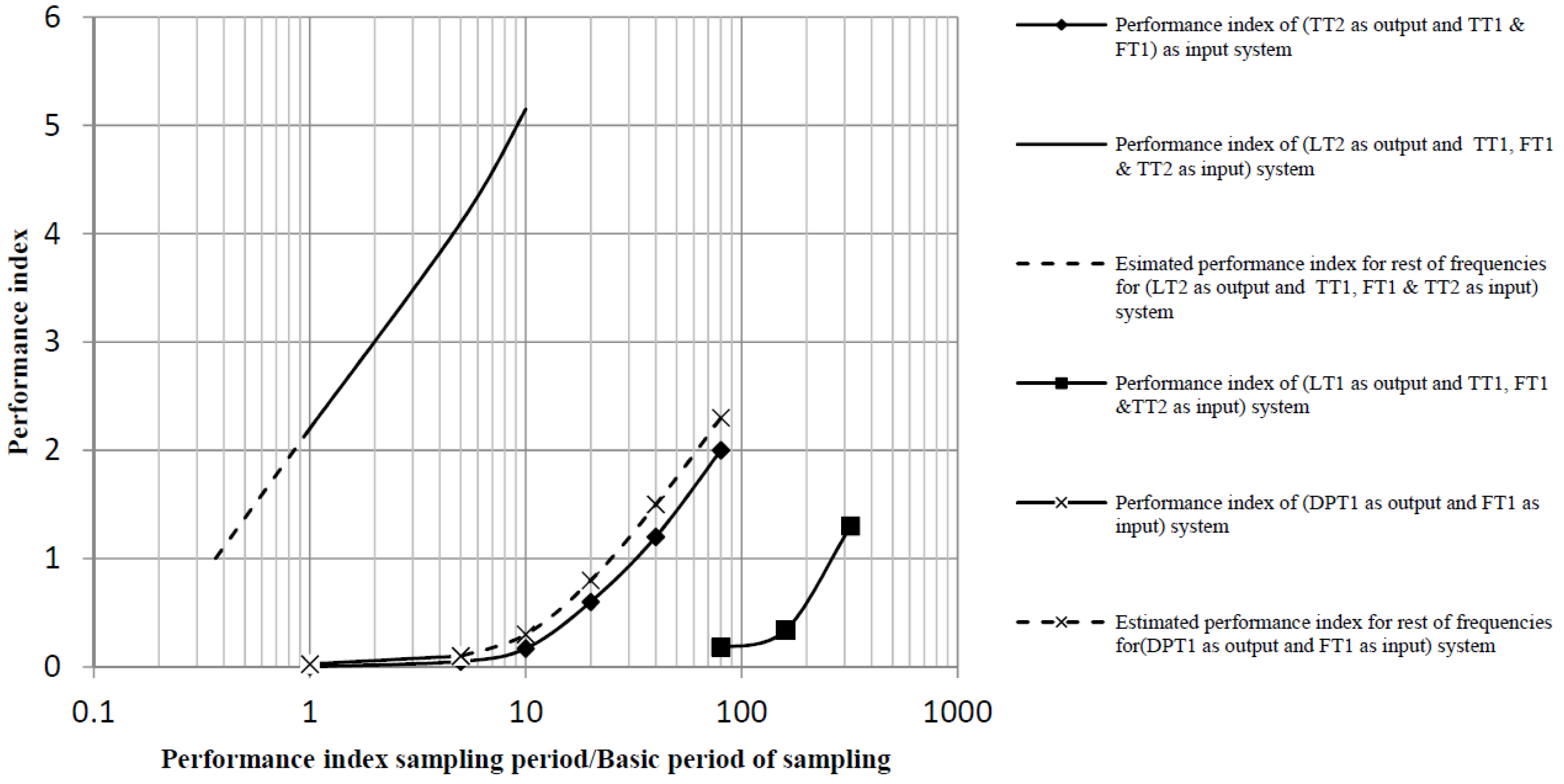
Figure 11.
Flowchart for obtaining best sampling rate for control, monitoring and historian purposes algorithm.
Figure 11.
Flowchart for obtaining best sampling rate for control, monitoring and historian purposes algorithm.

Figure 12.
A schematic of analog signal digitizing by hierarchical sampling rate: from the fastest (for controlling purpose) to the slowest (for historian purpose) sampling rates, a comparison between conventional methods and the proposed method.
Figure 12.
A schematic of analog signal digitizing by hierarchical sampling rate: from the fastest (for controlling purpose) to the slowest (for historian purpose) sampling rates, a comparison between conventional methods and the proposed method.

Figure 13.
Comparison of data size generated by different sampling-interval calculation methods in 90 min for controlling, monitoring and historian (for failure analysis) purposes.
Figure 13.
Comparison of data size generated by different sampling-interval calculation methods in 90 min for controlling, monitoring and historian (for failure analysis) purposes.

Figure 14.
An elementary link schedule showing a schedule for transmitter with an analog input, PID block, and a valve with an analog output block [16].
Figure 14.
An elementary link schedule showing a schedule for transmitter with an analog input, PID block, and a valve with an analog output block [16].


Table 1.
Overall cut-off frequency of process values in FFT analysis.
| Process Value Name | Cut-Off Frequency (Hz) | Absolute Mean Value of Variable | Maximum Value of FFT |
|---|---|---|---|
| DPT1 | 0.1008 | 0.1008 | |
| DPT2 | 0.1438 | 0.1438 | |
| DPT3 | 0.1827 | 0.1828 | |
| DPT4 | 0.1424 | 0.1424 | |
| FT1 | 220.2619 | 220.25 | |
| LT1 | 13.8186 | 13.82 | |
| LT2 | 3.3918 | 3.392 | |
| LT3 | 30.0275 | 30.03 | |
| PT1 | 65.6893 | 65.7 | |
| TT1 | 63.7867 | 63.8 | |
| TT2 | 33.6374 | 33.635 | |
| TT3 | 18.6766 | 18.675 | |
| TT4 | 21.1327 | 21.135 | |
| TT5 | 10.6754 | 10.675 |
Table 2.
Low and high cut-off frequencies for FFT analysis of process values deviation from mean value.
Table 2.
Low and high cut-off frequencies for FFT analysis of process values deviation from mean value.
| Process Value Name | Low Cut-Off Frequency (Hz) | High Cut-Off Frequency (Hz) | Maximum Value of FFT as a Percentage of Absolute Mean Value of Process Variable in Time Domain (%) |
|---|---|---|---|
| DPT1 | 0.0001 | 0.0002 | 1.19 |
| DPT2 | 0.0042 | 0.0048 | 0.97 |
| DPT3 | 0.0002 | 0.0088 | 0.93 |
| DPT4 | 0.0001 | 0.0089 | 0.70 |
| FT1 | 0.0001 | 0.0002 | 1.23 |
| LT1 | 0.0001 | 0.0003 | 7.81 |
| LT2 | 0.0001 | 0.0002 | 10.62 |
| LT3 | 0.0005 | 0.0007 | 0.47 |
| PT1 | 0.0001 | 0.0048 | 0.05 |
| TT1 | 0.0001 | 0.0002 | 0.16 |
| TT2 | 0.0001 | 0.0002 | 0.53 |
| TT3 | 0.0001 | 0.0002 | 1.43 |
| TT4 | 0.0001 | 0.0002 | 7.59 |
| TT5 | 0.0001 | 0.0002 | 1.78 |
Table 3.
Summarized auto-regressive moving average (ARMA) model parameters for the studied chemical process.
Table 3.
Summarized auto-regressive moving average (ARMA) model parameters for the studied chemical process.
| Subsystem | A | B | C | D |
|---|---|---|---|---|
| TT2 as output TT1 & FT1 as input (1, 1) | [1, −0.9981] | B1–78 = 0 B79 = −0.007830 | [1, 0.7830] | 1 |
| TT2 as output TT1 & FT1 as input (1, 2) | [1, −0.9981] | B1–54 = 0 B55 = −5.4282e−4 | [1, 0.7830] | 1 |
| LT2 as output TT1, FT1 & TT2 as input (1, 1) | [1, −0.3786] | B1–10 = 0 B11 = −0.0081 | [1, 0.8698] | 1 |
| LT2 as output TT1, FT1 & TT2 as input (1, 2) | [1, −0.3786] | B1–10 = 0 B11 = 0.0438 | [1, 0.8698] | 1 |
| LT2 as output TT1, FT1 & TT2 as input (1, 3) | [1, −0.3786] | B1–10 = 0 B11 = −0.0480 | [1, 0.8698] | 1 |
| LT1 as output TT1, FT1 & TT2 as input (1, 1) | [1, −0.9704] | B1–8 = 0 B9 = −0.0333 | [1, −0.4690] | 1 |
| LT1 as output TT1, FT1 & TT2 as input (1, 2) | [1, −0.9704] | B1–40 = 0 B41 = −0.0229 | [1,−0.4690] | 1 |
| LT1 as output TT1, FT1 & TT2 as input (1, 3) | [1, −0.9704] | B1–4 = 0 B5 = 0.0181 | [1, −0.4690] | 1 |
| DPT1 as output FT1 as input (1, 1) | [1, −0.9291] | B1–5 = 0 B6 = 0.0567 | [1, 0.7887] | 1 |
Table 4.
Comparison of different sampling-rate selection methods.
| Period of Sampling Rate (Sec) | |||||
|---|---|---|---|---|---|
| Existing Methods (Fixed Sampling Rates) | Methods Used in This Paper (Flexible Methods) | ||||
| Process parameter | API 554 recommendation | Åström & Wittenmark, recommendation [1] | Wavelet analysis (10% criteria) | Performance index analysis | |
| Controller | TT2 | 0.02 | 0.005 | ∞ | 6 |
| LT2 | 0.02 | 0.01 | 0.08 | 0.07 | |
| LT1 | 0.02 | 0.1 | 250 | 50 | |
| DPT1 | 0.02 | 0.005 | 16 | 5 | |
| Monitoring | TT2 | 1 | 1 | ∞ | 6 |
| LT2 | 1 | 1 | 0.08 | 0.07 | |
| LT1 | 1 | 1 | 250 | 50 | |
| DPT1 | 1 | 1 | 16 | 5 | |
| Historian Purpose | TT2 | <60 | 1 | ∞ | 6 |
| LT2 | <60 | 1 | 0.08 | 0.07 | |
| LT1 | <60 | 1 | 250 | 50 | |
| DPT1 | <60 | 1 | 16 | 5 | |
Table 5.
Data generated by each method for different applications in control and monitoring systems.
Table 5.
Data generated by each method for different applications in control and monitoring systems.
| Purpose | Controlling | Monitoring | Historian | |
|---|---|---|---|---|
| Method | ||||
| Proposed approach | 43,336 | 43,336 | 43,336 | |
| API 554 approach | 4,860,000 | 97,200 | 1260 | |
| Åström & Wittenmark recommendation | 14,742,000 | 97,200 | 97,200 | |
Table 6.
Summary of data size reduction for control, monitoring and data storage obtained by different methods.
Table 6.
Summary of data size reduction for control, monitoring and data storage obtained by different methods.
| Decreasing Percent | |||||||
|---|---|---|---|---|---|---|---|
| Controlling | Monitoring | Historian | Traffic of Industrial Network | ||||
| Sampling rate changing method | 99.11% of API 554 method | 99.71% of Åström & Wittenmark method | 55.42% of API 554 method | 55.42% in comparison with Åström & Wittenmark method | No decrease compared with API 554 method | 55.42% decrease compared with Åström & Wittenmark method | Associated with Hodson [16] method in comparison with existing methods in Foundation Fieldbus in Delta V system: 82% |
| Linear correlation method | 99.19% of API 554 method, associated with sampling rate method | 55.56% of API 554 method, using only this method. | 59.67% of API 554 method, associated with sampling rate method | 55.56% of API 554 method, using only this method. | No decrease in comparison with API 554 method, associated with sampling rate method | No decrease in comparison with all methods, using only this method. | Associated with Hodson [16] and sampling rate change method in comparison with existing methods in Foundation Fieldbus in Delta V system: 85% |
© 2020 by the authors. Licensee MDPI, Basel, Switzerland. This article is an open access article distributed under the terms and conditions of the Creative Commons Attribution (CC BY) license (http://creativecommons.org/licenses/by/4.0/).
Share and Cite
MDPI and ACS Style
Abbasinejad, R.; Hourfar, F.; Madhuranthakam, C.M.R.; Elkamel, A. A Data Size Reduction Approach Applicable in Process Control System of Oil and Gas Plants. Sustainability 2020, 12, 639. https://0-doi-org.brum.beds.ac.uk/10.3390/su12020639
AMA Style
Abbasinejad R, Hourfar F, Madhuranthakam CMR, Elkamel A. A Data Size Reduction Approach Applicable in Process Control System of Oil and Gas Plants. Sustainability. 2020; 12(2):639. https://0-doi-org.brum.beds.ac.uk/10.3390/su12020639
Chicago/Turabian StyleAbbasinejad, Reza, Farzad Hourfar, Chandra Mouli R Madhuranthakam, and Ali Elkamel. 2020. "A Data Size Reduction Approach Applicable in Process Control System of Oil and Gas Plants" Sustainability 12, no. 2: 639. https://0-doi-org.brum.beds.ac.uk/10.3390/su12020639
Note that from the first issue of 2016, this journal uses article numbers instead of page numbers. See further details here.