An Integrated Multi-Criteria and Multi-Objective Optimization Approach for Establishing the Transport Plan of Intercity Trains


Faculty of Transport, Technical University of Sofia, 8 Kl. Ohridski Blvd., 1000 Sofia, Bulgaria
Sustainability 2020, 12(2), 687; https://0-doi-org.brum.beds.ac.uk/10.3390/su12020687
Submission received: 2 January 2020
/
Revised: 9 January 2020
/
Accepted: 15 January 2020
/
Published: 17 January 2020
(This article belongs to the Special Issue Sustainable Railway System)
Abstract
:The development of the transport plan must take into account various criteria impacting the transport process. The main objective of the study is to propose an integrated approach to determine the transport plan of passenger trains. The methodology consists of five steps. In the first step, the criteria for optimization of the transport plan were defined. In the second step, variants of the transport plan were formulated. In the third step, the weights of the criteria are determined by applying the step-wise weight assessment ratio analysis method (SWARA) multi-criteria method. The multi-objective optimization was conducted in the fourth step. The following multi-objective optimization approaches were used and compared: weighted sum method (WSM), compromise programming method (CP), and the epsilon–constraint method (EC). The study proposes a modified epsilon–constraint method (MEC) by applying normalization of each objective function according to the maximal value of the solution by individual optimization for each objective function, and hybrid methods: hybrid WSM and EC, hybrid WSM and MEC, hybrid CP and EC, and Hybrid CP and MEC. The impact of the variation of passenger flows on the choice of an optimal transport plan was studied in the fifth step. The Laplace’s criterion, Hurwitz’s criterion, and Savage’s criterion were applied to come to a decision. The approbation of the methodology was demonstrated through the case study of Bulgaria’s railway network. Suitable variant of transport plan is proposed.
1. Introduction
The establishment of passenger train services is the most important task in railway operations planning and determines its sustainable development. The determination of the transport plan of intercity trains is an optimization problem that depends on different criteria affecting the transport process. Passenger train planning is related to the train timetable, rolling stocks planning, crew scheduling, and other operational parameters (trains stopping, railway vehicles circulation in passenger transport). The transport plan includes fixing the routes of intercity trains, the number of trains for each route (frequency of service), and the stations at which each train stops. Determining the transport plan by means of one criterion alone is not sufficient to meet the needs of both the passenger transport service and the carrier’s capabilities. Usually the basic criterion for determining the transport plan is transport costs. The effective planning for passenger services requires a complex view of passenger satisfaction and the possibilities of railway operators. The train frequency, journey time, safety, and reliability are the factors related to the convenience of passengers and their choice of transport. It is important to increase the effectiveness of decision making by taking into account different important criteria affecting the transport process when choosing a transport plan.
Multi-objective optimization allows us to minimize or maximize more than one objective function simultaneously. Each objective aims at a minimization or a maximization of a specific output. There are different multi-objective optimization (MOO) approaches such as the weightage method, epsilon-constraint method, compromise programming, genetics algorithms, differential evaluation, and others. MOO methods search for the set of optimal solutions that form the so-called Pareto front. So, a compromise solution between the various objectives has to be determined. Multi-objective optimization allows for a compilation of a mathematical model using the standard optimization algorithms for single-objective optimization.
The hypothesis of the study is that the transport plan of intercity trains depends on the economic and technological criteria related to transport, so the determination of an optimal compromise solution based on these criteria can help railway companies to make decisions about the improvement of railway transport services.
The present paper aims to propose an integrated approach based on the multi-criteria and multi-objective methods to develop a transport plan that takes into consideration the railway operator’s capabilities and passenger needs. The multi-criteria approach was used to determine the weights of the defined criteria related to transport. Multi-objective optimization was applied to solve a compromise solution of the transport scheme of intercity trains based on simultaneous application of defined objectives.
The methodology of the study includes: defining the criteria to assess the transport plan, determining the weights of the criteria by applying multi-criteria approach, applying different multi-objective modelling to determine the suitable transport plan, and experimentation of new hybrid approaches of multi-objective and multi-criteria methods.
The novelty of the proposed methodology and its main contribution consists of determining the criteria for assessment of the transport plan of passenger trains that take into account important factors for the railway company and passengers factors such as: operating cost of railway operator, travel time, stop-planning, reliability, capacity, operational speed, and directness; integration of the multi-criteria approach that define the importance of criteria with the multi-objective methods that determine the most suitable transport plan in railway networks; experimentation of a new modified epsilon-constraint method and also hybrid multi-criteria methods; verification of the results by applying different multi-objective methods. This study proposes new criteria for multi-objective optimization such as reliability indicated by the coefficient that accounted for the delays of trains, directness, and number of stops, which have not been studied in the literature.
The structure of the paper is as follows. First, Section 2 presents a literature review. Section 3 constructs a research methodology. Section 4 presents computational procedures and an analysis of the results. Finally, Section 5 presents the conclusions. The capabilities of the elaborated approach are illustrated through its application for the optimization of the transport plan of intercity trains in Bulgaria’s railway network considering several important indicators for transport process.
2. Literature Review
Mathematical programming methods were applied to the optimization of train planning. A single objective optimization is usually used, such as transport costs [1,2], time [3], or distance [4]. Multi-objective programming techniques provide the decision maker with a tool for considering the relative importance of the objectives as a single-objective approach.
A two-layer optimization model for high-speed railway was elaborated in [5]. The first model determined the service frequencies and achieved an optimal stop-schedule. The second model was based on mixed integer programming to maximize passenger volume and minimize the total travel time for all passengers. The model was experimented on Taiwan’s high-speed railway and also on the Beijing–Shanghai high-speed railway line in China. In [6] the authors proposed five factors: cost, speed, security, punctuality, and transport capacity to determine the advantages and disadvantages of each transport mode (railway, road, water, air, and pipeline). The Analytic Hierarchy Process (AHP) was applied to identify the best alternative. A multi-objective optimization model for railway route selection was elaborated on in [7]. The objectives included minimization of the train-running time, railway fare, transfer frequencies, distance between transfer stations, transfer interval time, and time to restore energy after fatigue. The two-phase algorithm for feasible routes taking into account the train timetable and information entropy was proposed. The model was tested for routes of China’s railway network. A multi-objective two-stage mixed-integer stochastic programming model for the design of transfer stations was elaborated on in [8]. The expected costs and the distance travelled by the vehicles were taken into account. The model used a parameter to describe the level of trade-off between the two objectives.
A multi-objective linear programming model was proposed to supply chain planning [9]. The authors introduced six objective functions connected to the economic objective, environmental objectives, and social objectives. An improved version of the augmented epsilon-constraint method was used to do the research.
A multi-objective train scheduling model aimed at the satisfaction of the railway company and the passengers was developed in [10]. The mathematical model included lowering the fuel consumption cost and shortening the total passenger-time. First, the epsilon-constraint method was applied for solving the problem. Using the obtained Pareto frontier, a detailed multi-objective optimization was performed using distance-based methods. The problem of the optimal allocation of passenger train services on an intercity high-speed rail line was studied in [11] based on a multi-objective programming model. The fuzzy approach was used for obtaining the best-compromise solution, including the train stop-schedule plan, service frequency, and fleet size. The authors used the following objectives in the model: minimizing the total operating cost for the operator and minimizing the passenger’s total travel time loss. The model was experimented on Taiwan’s high-speed rail system. The multi-objective mixed integer linear approach was applied to optimize both train stop planning and train scheduling problems, [12]. The linear weighted method was used. The total dwelling time at intermediate stations and total delay at origin station were the objectives for the model. The proposed model was experimented on the Beijing–Shanghai high-speed railway line. The train routing and train scheduling problem was solved by multi-objective optimization [13]. Three objective functions were listed: minimizing the average travel time of the trains, minimizing the traction energy consumption of the trains, and minimizing the total delayed times. The values of the weighted coefficients were determined by means of fitness function and sensitivity analysis.
An improved genetic algorithm based on train control and multi-objective optimization model was designed to solve train routing. A bi-level optimization model was formulated for transport network management, [14]. A genetic algorithm was used as a multi-objective method. The total network travel time, the total network flow, and the origin-destination pair accessibility were used as criteria of the optimization.
A multi-objective passenger railway transport plan optimization model was proposed in [15] based on minimization of the generalized travel time and minimization of the operating costs. The epsilon-constraint method was used to present a multi-objective problem into a single-objective problem. The model was experimented for SNCF Transilien (French railway operator for Parisian suburban mass transit). A time-energy-efficient model based on multi-objective optimization was introduced in [16]. The following three methods to transform the multi-objective model into a single-objective model were applied: linearly weighted compromise approach, ideal-point compromise approach, and fuzzy linear programming approach. A genetic algorithm and augmented max–min operator were designed to solve the problem.
A multi-modal routing problem was explored in [17]. The multi-objective optimization consisted of two objective functions, one of minimizing the generalized costs and the other of minimizing the social risk along the planned routes. The authors applied the normalized weighted sum method, to solve the optimization problem. The model was experimented on the Beijing–Tianjin–Hebei region in China. In [18], a multi-objective mixed integer programming model was proposed to study a routing problem. Two objectives were formed, one was minimization of total cost and the other objective was minimization of transport risk. The weighted sum method was applied to solve the problem by one objective function. The Pareto optimization and the Pareto frontier by normalized normal constraint method were used in [19] to study the multi-modal transport routing problem. The two objectives of the bi-objective optimization model were minimization of the total transport costs and total transport time.
A genetic algorithm was used to solve multi-objective model presented by two objectives: the expected total energy consumption and the total traversing time [20]. In [21], a multi-objective train-scheduling optimization model was elaborated for the minimization of both the operation costs and trip time. Fuzzy mathematical programing was applied to solve the multi-objective problem. In [22], a new multi-objective approach with examples of two and three objectives was studied. The bi-objective model included minimization of the transport cost and time, and the three objective models took into account the minimization of transport cost, time, and damage cost. A weighted goal programming model was proposed that helps to obtain the multiple solution points by using different weights.
In [23], the authors solved a bi-objective transport problem, minimizing the total transport cost and delivery time by using the distance method of lexicographic goal programming. A similar approach was used also in [24]. A weighted goal programming model was proposed. A new multi-objective periodic railway timetabling problem was elaborated in [25]. Four objectives for minimization were considered, such as train journey time, timetable regularity deviation, timetable vulnerability, and the number of overtaking. The epsilon-constraint method was applied to solve the multi-objective model. The trade-offs solution for the four objectives were determined by using standardized Euclidean distance and applying an additional indicator as the capacity utilization. The approbation of the model was made for a Dutch railway corridor.
Rail passenger safety and comfort system was presented as a multi-objective optimization problem in [26]. The following objectives were proposed: functionality and upgradeability, compliance with standards, and costs. A new hybrid method based on the weighted sum and epsilon-constraint methods was proposed. A multi-objective high-speed rail passenger fares optimization problem was developed in [27]. The profit and passenger welfare were tested as objectives. The epsilon-constraint method and lexicographic optimization approach were used. The computational experiments were formed for the Beijing–Shanghai regional network.
The route choice of travelers was presented by a multi-objective model including the travel time and travel costs [28]. The authors developed heuristic solution methods to solve the model. A multi-objective transport problem was formulated in [29], where the authors optimized transport time and the cost function. An optimal (compromise) solution was determined that minimizes the total time without considering the objective function of time in the model, and also sustainable development was considered by minimizing the pollution factor. A goal programming method was applied.
It may be concluded that the following problems were studied: railway route planning, design of transfer stations, supply chain planning, passenger train service, stop planning, train schedule planning, train routing, and transport planning. Most authors consider the main criteria as the operating cost and time travel, which has a great importance for developing the transport plan of the trains, [11,15,19,21,22,23,24,29]. Some authors also investigated the criteria of transfer interval time [7], delayed times [13], social risk [17], transport risk [18], total energy consumption [20], damage cost [22], functionality and upgradeability, number of overtaking [25], compliance with standards [26], and the pollution factor [29]. The choice of criteria depends of the object of the study. It is necessary when elaborating the transport plan of passenger trains to apply criteria related to the transport process. The impact of the directness of the passenger trains was not studied. The number of stops and train delays are also important technological indices that could be studied. On the other hand, it is also important to examine the impact of changing passenger traffic on the choice of transport plan.
The authors used a multi-criteria approach such as AHP method [6] or MOO. To summarize, the following multi-objective methods that were applied: epsilon-constraint method [9,10,15,25,27], lexicographical approach [23], fuzzy approach [11,16,21], WSM [12,17,19,22], genetic algorithm [13,14,19,20], and hybrid method WSM and epsilon-constraint [26]. Epsilon-constraint method and WSM were used most by the authors. Usually, when using the epsilon-constraint method, the most important criterion was determined by the decision maker, without determining the weight of the criteria. The hybrid methods were not sufficiently studied in literature.
The MOO could serve as a tool to determine the suitable solution depending on different criteria. In this study three different multi-objective methods are proposed and a new modified epsilon-constraint method is experimented.
The elaboration of the transport plan serves different purposes and it is important for the development and attractiveness of railway transport. It can be summarized that transport planning is aimed at dealing with the following problems: technological-service frequencies, stop-schedule, distance travelled; economic-operating costs, railway fare; social-transport and convenience of the passengers; integrated-satisfaction of the railway company and passengers.
3. Materials and Methods
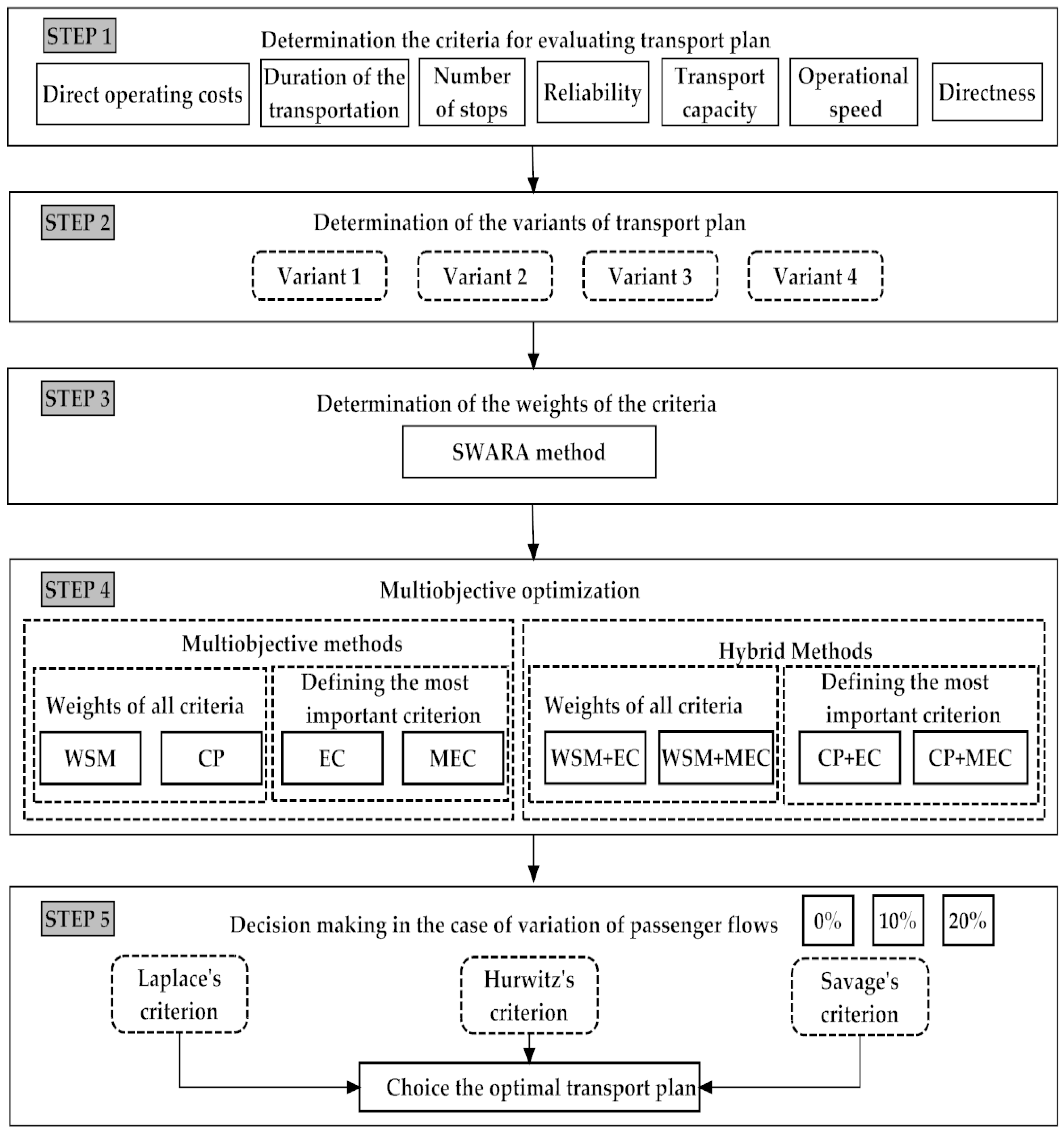
The methodology is illustrated in Figure 1.
The methodology includes the following five steps:
- In the first step, the criteria for optimization of the transport plan of passenger trains are defined.
- In the second step, the variants of transport plan are formed. The variants include the categories of passenger trains, the number of wagons in the train composition, and the number of itineraries of the trains.
- In the third step, the weights of the criteria are determined by applying the step-wise weight assessment ratio analysis method (SWARA) method.
- In the fourth step, the multi-objective optimization is made. The following multi-objective optimization approaches are used and compared:
- ○
- Multi-objective optimization by using the weighted sum method (WSM). The method transforms multiple objectives into an aggregated objective function by multiplying each objective function by a weight. Each single objective optimization determines a different optimal solution on the Pareto front. The solution obtained by WSM approximates the Pareto front.
- ○
- Multi-objective optimization using compromise programming method (CP).
- ○
- Both methods use the results obtained for the weights of the criteria by SWARA method.
- ○
- Multi-objective optimization using epsilon–constraint method (EC).
- ○
- Multi-objective optimization using modified epsilon–constraint method (MEC).
- ○
- Multi-objective optimization through hybrid methods: hybrid WSM and EC; hybrid WSM and MEC; hybrid CP and EC; hybrid CP and MEC.
- In the fifth step the variation of values of passenger flows is studied. The choice of the suitable variant of transport plan is made.
3.1. Step 1: Determination of the Criteria for Optimization
Table 1 presents the criteria to determine the optimal transport plan for a variant scheme of organization of passenger trains. These criteria are related to the capabilities of the transport operator and the requirements of passengers for transport.
The coefficient of reliability is determined as follows:
where: is the number of delayed trains from itinerary i, trains /day; is the number of trains from itinerary i, trains /day.
In this study the train capacity and speed are accounted for by coefficients to minimize the optimization functions for these criteria.
The coefficient representing the transport capacity is determined as follows:
where: is the number of seats on a train of itinerary i
The coefficient representing the average speed is determined as:
The coefficient representing the number of stops per kilometer for itinerary i.
where: is the length of the itinerary i, km.
3.2. Step 2: Determination of the Variants of Transport Plan of Passenger Trains
The transport plan includes the number of categories of trains and number of trains for each category by itinerary. The variant schemes could be formed taking into account the number of wagons in train composition and the number of categories of trains.
3.3. Step 3: Determination of the Weights of Criteria by the SWARA Method
The SWARA method is an easy and powerful tool that uses experts to evaluate the criteria. The method is based on experts’ assessment of the comparative importance of criteria and recalculated weights. SWARA does not use a scale for evaluation. The method consists of the following steps [30]:
- The expert ranks the criteria in descending order of their expected significance.
- Determination of the comparative importance of average values For this purpose starting from the second criterion the expert assesses the relative importance of criterion to the previous criterion.
- Determination of the value of coefficient
- Determination of the recalculated weight :
- Calculation of the weight of criteria as follows:where: —represents the relative weight of the criteria.
For the weights the following condition must to be met:
To determine the consistency of the experts’ assessment in the study the Spearman Rank correlation coefficient is proposed, Ref. [22].
where is the Spearman Rank correlation coefficient; is the distance between the ranks for each , data pairs, n is the number of elements in each data series (i.e., number of criteria).
This approach allows us to determine the correlation between the evaluations obtained by experts.
3.4. Step 4: Multi-Objective Optimization
The multi-objective optimization problem is as follow:
Subject to:
where: is the number of itineraries in railway network; is the number of trains for itinerary , train/day; is the passenger train capacity utilization coefficient; is the coefficients that take into account the possibility of passenger train on route to serve the section formed between two adjacent stations and ; is the passenger flow in a section formed between two adjacent stations and , who will use trains on itinerary , pass./day; is the maximum capacity of the railway line between two adjacent stations and which is being examined, train/day; is the minimal number of trains for itinerary , train/day.
The objective functions (11)–(17) are linear and define the optimal transport plan. Condition (18) means ensuring a seat for each passenger on any section of the railway network. Condition (19) means that the number of trains must not exceed the maximum capacity of the railway line. Condition (20) ensures the realization of the frequency of certain transport links for some routes, serving major transport and administrative hubs. Condition (21) means that the number of trains must be positive and integer.
The multi-objective optimization by WSM converts objective functions into scalar-based objective functions by defining them as weighted sums of various objectives, Ref. [31,32,33].
The multi-objective optimization model by WSM is defined as follow:
Subject to:
and condition (18)–(22).
where: is the number of optimization function in multi-objective linear optimization model; is the weight of j-th optimization function; is the normalized value of j-th optimization function.
The objective functions are of different nature and that is the reason why the normalization method is applied. The normalization is made according to the maximal value of objective functions.
The multi-objective optimization model by compromise programming (CP) method defines the best/suitable solution based on the shortest distance from the reference point (i.e., ideal solution).
The criterion of optimization is as follows, [19]:
and conditions (18)–(22), and (24).
where: is a metric for optimal solution, is the ideal value of criterion j (in the case of minimization this is the minimal value of criterion, is the anti-ideal point for the j-th objective (in the case of minimization this is the maximal value of the solutions—, is a parameter that is used to present the attitude of the decision-maker with respect to compensation between deviations; p = 1 is the so-called street-block distance, or Manhattan distance; p = 2, it is represents the Euclidean distance; p = , it is Tchebyshev distance, and correspond to min-max problem. The value of p = 1 has used in the study as the problem could be solved by linear programming.
The epsilon-constraint method optimizes one of objective functions by using the other objective functions as constraints, [31,32]. The criterion that presents the objective function is determined by a decision maker who defines it as more important than the other ones. The determination of the importance of objective functions can be made also by the determined weights of criteria using the SWARA method. For example, the multi-objective optimization model by the epsilon-constraint method is structured by placing the objective operational costs as the objective function, while the other six are placed as the additional constraints along with the existing constraints as follows:
Subject to:
and conditions (18)–(22)
where: is the bound of objective j.
The values of can be determined using the solution of each objective function j, or can be set by a decision maker. In the study, is determined by using the maximum value of objective function j obtained by individual optimization.
In this study, a modified epsilon-constraint method is purposed using normalization of each objective function. The normalization is made using the maximum value of the solution by individual optimization for each objective function. The choice which function j to represent as an objective is performed as in the EC method. For example, MEC apply like EC for an objective function the operational costs .
The multi-objective optimization model by using the modified epsilon-constraint method is presented as follows:
Subject to:
and conditions (18–22).
The multi-objective optimization models by using the hybrid methods are formed as follows:
- Hybrid WSM and EC—it uses objective function (23) and conditions (24), (18)–(22), (28)–(33), and:
- Hybrid WSM and MEC—it uses objective function (23) and conditions(24), (18)–(22), (36)–(41), and:
- Hybrid CP and EC—it uses objective function (26), and conditions (24), (18)–(22), (28)–(33), and (42).
- Hybrid CP and MEC—it uses objective function (26) and conditions (24), (18)–(22), (36)–(41), and (43).
To determine the optimal transport plan, the variant schemes of transport are defined and compared. Each variant scheme is optimized by multi-objective optimization models.
The herein presented multi-objective optimization models are linear and can be solved by using linear optimization.
The optimal transport plan is determined as follows:
where: is the number of variant schemes, is the value of optimization function given by multi-objective optimization.
3.5. Step 5: Decision Making in the State of Variation of Passenger Flows
In this case, the best transport plan is determined taking into account the uncertainty of passenger flows. The decision matrix is formed according to the number of variations of passenger flows (and the number of variants of transport plan (.
In the study Laplace’s criterion, Hurwitz’s criterion and Savage criterion are proposed to make decisions [23].
Laplace’s criterion is based on the principle that all events are equal. The criterion of choosing an optimal transport plan in the case of minimum of multi-objective optimization is:
Hurwitz’s criterion uses the coefficient of optimism that allows for making a decision depending on different decision approaches. The value of can be set between 0 and 1. Generally, . While = 1 represents an optimistic approach, represents a totally pessimistic approach.
The optimal alternative in the case of minimum of multi-objective optimization is determined as:
Savage’s criterion represents the regrets of the decision maker of the possibility to obtain non-optimal results. The regret matrix is construed with the following elements in the case of minimum of multi-objective optimization:
where: k is the minimal value of column q.
The newly-formed matrix represents a loss and therefore only for it the minimax criterion can be applied. To apply the mini-max criterion, the maximum element by rows for each variant of transport plan of the new matrix is determined. Optimal is the variant for which the maximum value of criterion is the smallest, i.e.:
4. Results and Discussion. A Case Study of the Bulgarian Railway Network
4.1. Defining the Variants of the Transport Plan
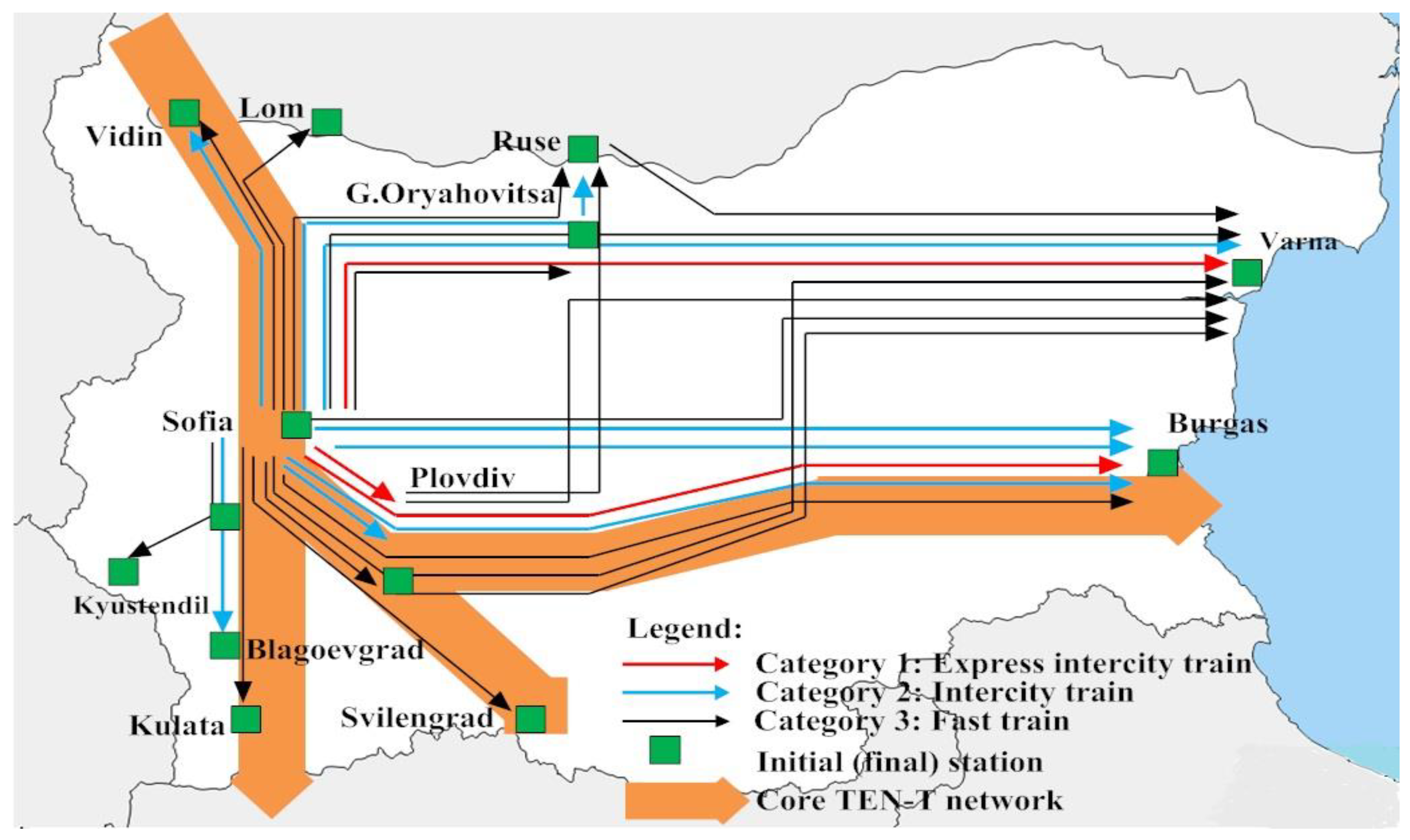
The herein presented multi-objective approaches are applied to Bulgaria’s railway network in order to investigate the transport plan of intercity trains. The itineraries include sections of Orient/East-Med TEN-T railway core corridor passing across Bulgaria and also a compressive railway network. Four variants of transport of passenger trains were examined in the study. The variants differ according to train categories and number of wagons in the train compositions. The following categories of passenger trains were examined: category 1—refers to express intercity trains with a reduced number of stops, reservation is needed; category 2—intercity trains that stopped in additional big transport centers and administrative centers as compared to category 1, reservation is needed; category 3—fast trains that serve additional intermediate stations between cities, big transport and important administrative centers compared to category 2. The study included two types of train composition according to the number of wagons with 3 or 4 wagons. The following variants of train composition are formed: express intercity trains (category 1) with 3 wagons or 4 wagons, intercity trains (category 2) with 3 wagons or 4 wagons, and fast train (category 3) with 4 wagons. The following number of itineraries in Bulgaria’s railway network were examined: category 1–3 itineraries; category 2–7 itineraries, category 3–17 itineraries.
The following variants of transport plan were examined:
- Variant 1 includes three categories of trains. Train category 1 includes 3 wagons; category 2 and category 3 include 4 wagons.
- Variant 2 includes also three categories of trains composed by 4 wagons.
- Variant 3 includes two categories of trains – category 2 composed by 3 wagons and category 3 composed by 4 wagons.
- Variant 4 is formed with train category 2 and category 3; both are composed of 4 wagons.
Figure 2 presents a scheme of categories of trains and itineraries for the Bulgarian railway network.
Table 2 presents the examined variants. The first row in the Table 2 shows the categories of passenger trains examined, the second row shows the number of wagons in the train composition for the respective train category, and the third row presents the number of investigated itineraries for each train category.
4.2. Determination of the Weights of Criteria
In the third step of the methodology assessments of the criteria weights by SWARA method, they were given by nine experts. Table 3 presents the values of comparative importance and weights for each expert. The end of the table shows the average values of weights obtained by the SWARA method.
The selection of the experts was conducted according to their experience in railway transport and the positions they hold in the Ministry of Transport, Information Technology, and Communications, or in the railway operator; scientific and research experience in the field of railway transport in academia. The experts independently of each other evaluated the comparative importance . The final weights are determined as average values of expert assessment.
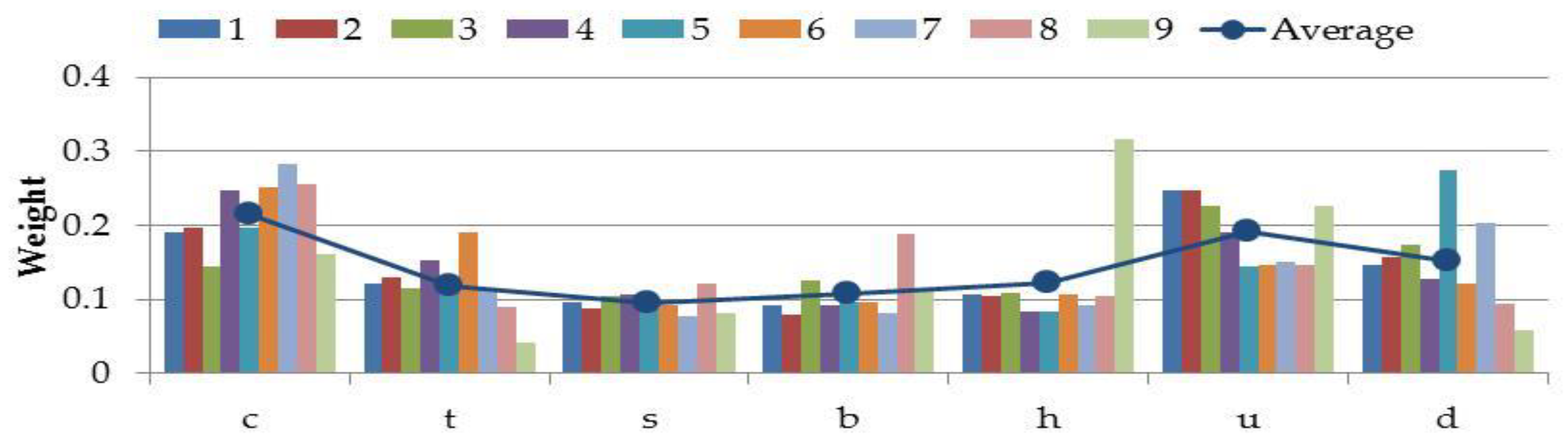
Figure 3 presents the comparison of experts’ assessment for each of the criteria and the average value of criteria weights. It can be seen that most important are the criteria: direct operating costs (), average speed (), and directness of transport ().
Table 4 presents the Spearman Rank Correlation coefficients between experts’ evaluations. The last row and the last column in the table show the values of Spearman rank correlation coefficients between the average value of weights and each of the experts’ assessment.
It can be seen that there is a different correlation between the experts’ evaluations and its average score. The results show that the scores of seven experts have strong correlation with the average value of weights ( is between 0.7 and 1); the scores of two experts have moderate strength of the correlation ( is between 0.4 and 0.5).
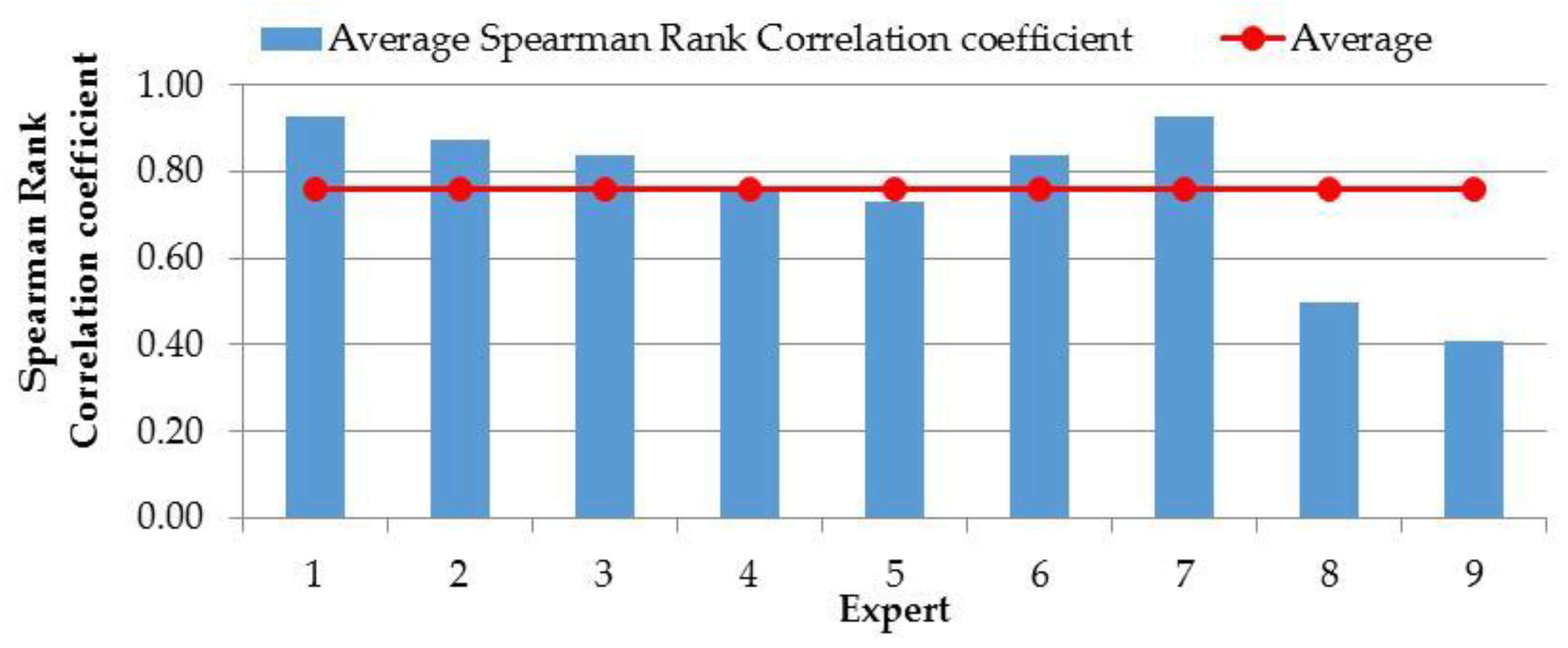
Figure 4 presents a comparison of values of average Spearman rank correlation coefficient for each of the experts (the last column in Table 4) and average value of Spearman rank correlation coefficient of experts’ assessment. The average value of Spearman rank correlation coefficient is determined by dividing the sum in last column of Table 4 by the number of experts, (0.76). It could be concluded that there is a strong correlation between experts’ assessment and the average weights.
4.3. Multi-Objective Optimization
The multi-objective optimization was conducted according to the proposed methodology.
Table 5, Table 6, Table 7 and Table 8 present the results of individual optimizations by each of objective functions from (11) to (17) subject to restrictive conditions from (18) to (22). The diagonal elements of the tables in bold show the solution of each objective function presented in the first column. The other modified elements of the tables present the solution according to the criteria given in the first row of the tables.
To determine the modified elements of the tables the following procedures are made:
- Let be the results of linear optimization of objective function (11) and restrictive conditions from (18) to (22) presented minimum of operational costs. The result of the objective function is presented in the first cell of diagonal elements of Table 5, Table 6, Table 7 and Table 8. For example, in Table 5 the value is 25,367.00 EUR/day. The modified results for values of objective function for others criteria are determined as follows:
- Let be the results of linear optimization of objective function (12) and restrictive conditions from (18) to (22) presented the minimum duration of the transport. The result of the objective function is presented in the second cell of diagonal elements of Table 5, Table 6, Table 7 and Table 8. For example, in Table 5 the value is 19,020.00 minutes/day. The modified results for values of objective function for other criteria are determined as follows:
- The same procedure is repeated for the other criteria.
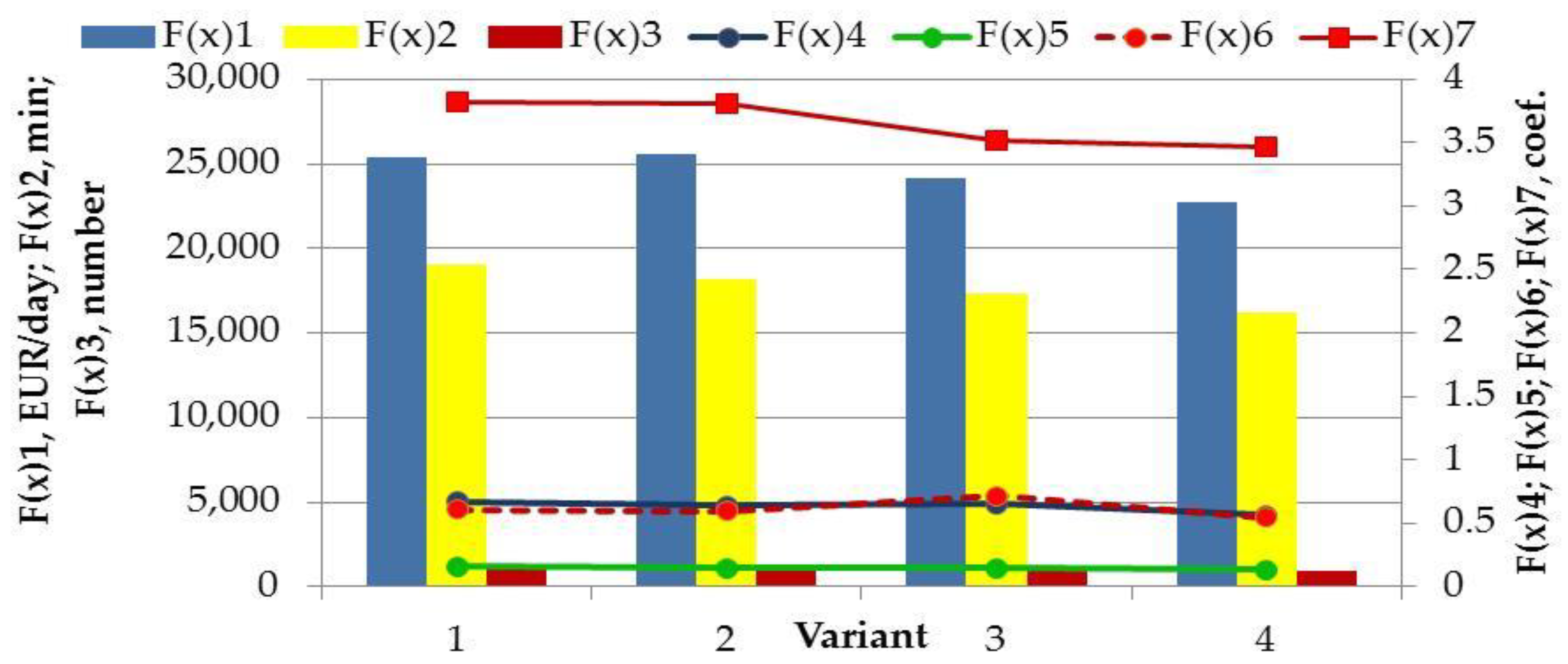
Figure 5 presents the comparison of solution by individual optimization for studied variants. The values are given in the diagonal elements of Table 5, Table 6, Table 7 and Table 8. It can be seen that for all individual optimization the optimal is Variant 4 of the transport plan.
The multi-objective optimization models presented in the methodology were applied to examine the different variants of the transport plan. Table 9 shows the results of the different approaches. The numbers in bold indicate the optimal values. It can be seen that for most multi-objective optimization models, the optimal transport plan is Variant 2. The epsilon-constraint method is an exception: the optimal solution is Variant 4. This result was equal to the solutions obtained through individual optimizations using direct operating costs. It could be seen in the results given in Table 8 and Table 9. The results presented through WSM and hybrid methods with WSM are equal. The results obtained by using CP and hybrid methods with CP are also similar. This indicates that the additional restrictions imposed on the WSM and CP did not affect the decision. The most important objective function for EC and MEC methods were determined according to the results of weights of criteria calculated by the SWARA method. It was found out that the objective direct operational costs had the greatest impact. The results from the epsilon-constraint method and modified epsilon-constraint method proposed in the study are different. The modified epsilon-constraint method gives similar results in regard to the optimal variant (Variant 2) as WSM and CP methods. It could be concluded that Variant 2 is most suitable for transport plan of intercity trains.
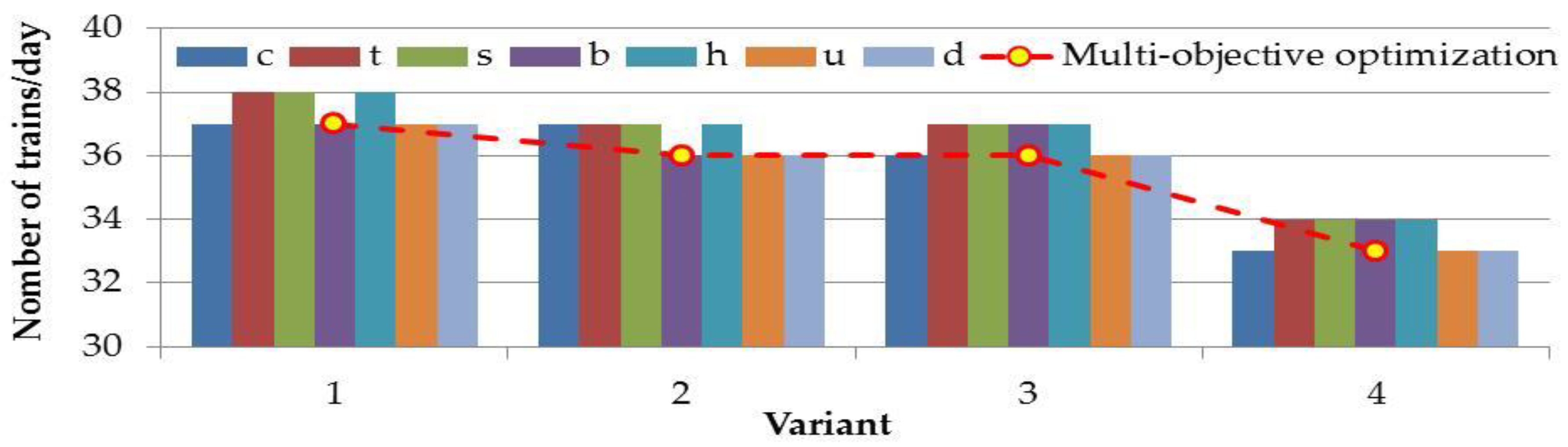
Figure 6 presents the comparison of the number of trains in the transport plan for all variants according to the individual optimizations and multi-objective methods. The results about the number of trains for different multi-objective approaches are similar.
It could be seen that the number of trains for Variant 2 is 37, and the number of trains for Variant 4 is 33. The value of the direct operational costs corresponding to the results of the number of trains given by WSM, CP, and MEC are 24,973.00 EUR/day. This value has been determined by multiplication of the results for number of trains for each itinerary by the relevant direct operational costs. The value of the direct operational costs for Variant 4 given by using the individual optimization, and by using EC method presented in Table 8 and Table 9 is respectively 22,715.00 EUR/day. It could be concluded that the application of proposed integrated multi-criteria and multi-objective optimization approach for establishing the transport plan of intercity trains allows for an increase in the train transport service with a minimum increase in transport costs (about 9%) as compared to the optimal variant, determined only by the criterion of minimum direct operating costs. This approach makes it possible to take into account not only the direct operating costs, but also the additional technological factors related to the transport process.
Sensitivity analysis was conducted to determine the limits of changing the weights of the criteria while preserving the optimal solution by WSM and CP (these methods use the criteria’s weights). Table 10 shows the lower and upper limits of the weights.
It can be seen that the criteria direct operating costs (c), operational speed (u), and directness (d) have a larger weight stability interval. It indicates that it could have a large effect on optimization.
The study shows that the following approaches for selecting the multi-objective method could be determined:
- Application of all specified criteria weights in multi-objective optimization. In this case it is recommended to apply WSM or CP to select the appropriate transport plan.
- The criterion with maximal importance (weight) is applied as objective function. The other criteria are included in the restrictive conditions of the multi-objective model. In this approach the weights of the criteria are not used in multi-objective optimization. In this case it is recommended to apply the MEC method.
An advantage of the study is the application of multi-criteria analysis to determine the most important criterion which is used for the objective function, and also the weights of criteria.
4.4. Decision Making in the State of Variation of Passenger Flows
The impact of the variation of passenger flows on choosing the optimal transport plan was studied by applying the Laplace’s, Hurwitz’s, and Savage’s criteria for decision making. Three variants of increment of passenger flows were compared—0%, 10% and 20%. The results are presented in Table 11, Table 12 and Table 13. The formulas (45), (46), and (48) are applied.
Table 11, Table 12 and Table 13 consist of two parts. The first part shows the results obtained for the objective function by using WSM, CP, and MEC. The second part presents the values of the criteria for decision making. The numbers in bold indicate the optimal values.
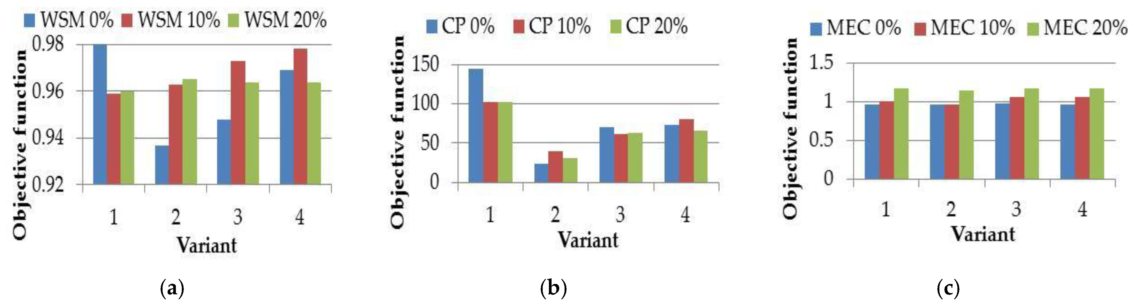
Figure 7 presents the comparison of values of objective function by different multi-objective optimizations and different variation in passenger flows.
It can be seen that when changing the values of passenger flows, the optimal variant of the transport plan is different. The results given by WSM show a change in the optimal transport plan when increasing passenger flows from Variant 2 to Variant 1. The results obtained by using the CP and MEC methods indicate persistence in the results. It could be concluded that the optimal variant for all changes in passenger flows is Variant 2.
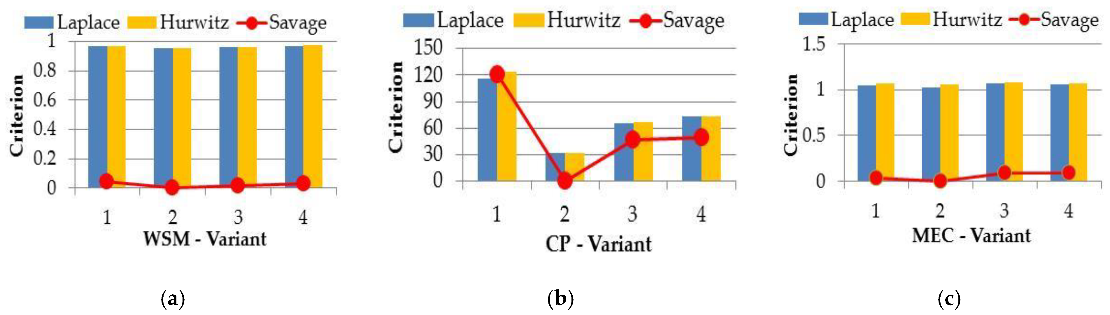
The application of the criteria for decision making makes it possible to choose the optimal transport plan in the case of uncertainty. The results of the optimal variant are similar by using the proposed criteria. The solution is also saved when the coefficient of optimism for Hurwitz’s criterion is changed.
Figure 8 presents a comparison of variants of the transport plan according to the criteria of decision making. For Hurwitz’s criterion, the value of is presented. The main advantage of Laplace’s criterion is its easy way of determining the best variant. The main advantage of Hurwitz’s criterion is the application of a parameter that allows for the variability of the results to be examined.
5. Conclusions
This research studied a combined SWARA multi-criteria method and multi-objective optimization approach to optimize the transport plan of passenger trains in the railway network. The variants of transport plan have been defined according to the stops and the number of wagons in the train compositions. The criteria of multi-objective optimization have been defined. The SWARA method has been applied to determine the weights of the criteria. The Spearman rank correlation coefficient has been applied to evaluate the expert assessments. The study showed that the direct operating costs (c = 0.21), operational speed (u = 0.19), and directness of transport (d = 0.15) are of main importance when determining a transport plan. Four variants of transport plan of intercity passenger trains were examined for the Bulgarian railway network. Different multi-objective optimization approaches were studied, such as WSM, CP, EC, and hybrid methods. WSM and the CP methods use weights of criteria in the objective function. The modified EC method was proposed. The determined weights by the SWARA method were applied in the WSM, CP, and hybrid methods. EC and MEC methods use the weights of criteria as a means to determine the criterion and objective function respectively with greatest importance. It was found out that all investigated approaches, except the EC method, give similar results with respect to the optimal variant. The optimal transport plan obtained by the EC method is similar to those given by individual optimizations. The modified epsilon-constraint method gives similar results with respect to the optimal variant like the WSM and CP methods.
The hybrid method formed through the integration of WSM, or CP with EC or MEC have been investigated. It was found out that the results are equal as the independent application of the relevant multi-objective method.
The impact of the variation of passenger flows on the choice of optimal transport plan was studied. Laplace’s criterion, Hurwitz’s criterion, and Savage’s criterion were applied to decision making. The WSM, CP, and MEC were used for studying the change in passenger flows. The determination of the optimal transport plan by different approaches serves to verify the obtained results.
By using the proposed multi-criteria and multi-objective optimization approach it was found out that the optimal variant of transport plan of intercity trains on the Bulgarian railway network is Variant 2 that included three categories of intercity trains composed with four wagons. The sensitivity analysis showed that the criteria of direct operating costs, operational speed, and directness have a larger weight stability interval to save the optimal variant. The optimal variant was also preserved with the studied increase in passenger flow of up to 20%. The application of the proposed integrated multi-criteria and multi-objective optimization approach for establishing the transport plan of intercity trains allows for an increase in the train transport service with a minimum increase in transport costs (of about 9%) as compared to the optimal variant, determined only by the criterion of minimum direct operating costs.
The main benefit of this study is the integration of a multi-criteria and multi-objective approach as a five step methodology to make a decision regarding the transport plan of passenger trains in the state of certainty and uncertainty of passenger flows. The multi-criteria approach allows us to determine the weights of the criteria and to define variants of the transport plan. The proposed criteria are important for railway companies and passenger requirements. In this study we have investigated not only the operating costs and time travel that are the preferred criteria in the literature, but also new criteria for multi-objective optimization, such as directness, number of stops, and reliability given by coefficient that accounted for the delays of trains, which have not been studied in the literature. The multi-objective approach defines an optimization problem that involves multiple objective functions in order to determine the appropriate solution. The weights assigned to the objectives, as well as the most important objective function, are determined by means of the multi-criteria approach. Each of the variants is optimized by using the multi-objective optimization models. The optimal transport plan in the state of certainty is determined according to the minimum value of multi-objective functions. In the state of uncertainty, multi-objective optimization models for different variations of passenger flows for each of the variants are solved. On the basis of the criteria for decision making, the suitable transport plan was determined.
The proposed methodology could serve in the decision-making process for transport plan selection and route planning in situations related to change in passenger traffic.
Funding
This research was supported by contract №KП-06-H27/12 of 11.12.2018 “Modeling and elaboration of complex system for selection of transport technology in transport network” funded by the National Science Fund of the Ministry of Education and Science of Bulgaria.
Acknowledgments
Thanks to “BDZ Passenger Services” Ltd. for providing the data used in this study.
Conflicts of Interest
The author declares no conflict of interest.
References
- Goossens, J.H.M.; van Hoesel, S.; Kroon, L.G. On solving multi-type railway line planning problems. Eur. J. Oper. Res. 2006, 168, 403–424. [Google Scholar] [CrossRef]
- Schöbel, A. Line planning in public transportation models and methods. OR Spectr. 2012, 34, 491–510. [Google Scholar] [CrossRef] [Green Version]
- Schöbel, A.; Scholl, S. Line Planning with Minimal Traveling Time. In Proceedings of the 5th Workshop on Algorithmic Methods and Models for Optimization of Railways, Palma de Mallorca, Spain, 14 September 2005; pp. 1–16. Available online: https://drops.dagstuhl.de/opus/volltexte/2006/660/ (accessed on 15 December 2019).
- Jin, J.G.; Zhao, J.; Lee, D.H. A column generation based approach for the Train Network Design Optimization problem. Transp. Res. Part E Logist. Transp. Rev. 2013, 50, 1–17. [Google Scholar] [CrossRef]
- Wang, L.; Jia, L.; Qin, Y.; Xu, J.; Mo, W. A Two-Layer Optimization Model for High-Speed Railway Line Planning. In Advances in High-speed Rail Technology; China’s High-Speed Rail Technology, Fang, Y., Zhang, Y., Eds.; Springer: Singapore, 2018; pp. 447–465. [Google Scholar] [CrossRef]
- Xukuo, G.; Qiong, W. Research on the mode of present transportation in China and the analysis of railway transportation. In Proceedings of the 6th International Conference on Information Management, Innovation Management and Industrial Engineering, Xi’an, China, 23–24 November 2013; pp. 414–416. [Google Scholar] [CrossRef]
- Xinfeng, Y.; Lanfen, L.; Yinzhen, L.; Ruichun, H. Route Selection for Railway Passengers: A Multi-objective Model and Optimization Algorithm. J. Transp. Syst. Eng. Inf. Technol. 2013, 13, 72–78. [Google Scholar] [CrossRef]
- Kudela, J.; Somplak, R.; Nevrly, V.; Lipovsk, T.; Smejkalov, V.; Dobrovsky, L. Multi-objective strategic waste transfer station planning. J. Clean. Prod. 2019, 230, 1294–1304. [Google Scholar] [CrossRef]
- Vafaeenezhad, T.; Tavakkoli-Moghaddam, R.; Cheikhrouhou, N. Multi-objective mathematical modeling for sustainable supply chain management in the paper industry. Comput. Ind. Eng. 2019, 135, 1092–1102. [Google Scholar] [CrossRef]
- Ghoseiri, K.; Szidarovszky, F.; Asgharpour, M.J. A multi-objective train scheduling model and solution. Transp. Res. Part B 2004, 38, 927–952. [Google Scholar] [CrossRef]
- Chang, Y.-H.; Yeh, C.-H.; Shen, C.-C. A multi-objective model for passenger train services planning: Application to Taiwan’s high-speed rail line. Transp. Res. Part B 2000, 34, 91–106. [Google Scholar] [CrossRef]
- Yang, L.; Qi, J.; Li, S.; Gao, Y. Collaborative optimization for train scheduling and train stop planning on high-speed railways. Omega 2016, 64, 57–76. [Google Scholar] [CrossRef]
- Sun, Y.; Cao, C.; Wu, C. Multi-objective optimization of train routing problem combined with train scheduling on a high-speed railway network. Transp. Res. Part C 2014, 44, 1–20. [Google Scholar] [CrossRef]
- Konstantinidou, M.A.; Kepaptsoglou, K.L.; Stathopoulos, A. A Multi-objective Network Design Model for Post-disaster Transportation Network management. Promet-Traffic Transp. 2019, 31, 11–23. [Google Scholar] [CrossRef] [Green Version]
- Brethome, L.; Bouvet-Agnelli, C.; Chevrier, R.; van Oort, N.; Rodriguez, J. Optimization of a Passenger Railway Transportation Plan Considering Mobility Flows and Service Quality. 2017. Available online: http://resolver.tudelft.nl/uuid:e668596d-e4e7-4d53-880c-d774733fef83 (accessed on 15 December 2019).
- Xu, X.; Li, K.; Li, X. A multi-objective subway timetable optimization approach with minimum passenger time and energy consumption. J. Adv. Transp. 2016, 50, 69–95. [Google Scholar] [CrossRef]
- Sun, Y.; Lang, M.; Wang, D. Bi-Objective Modelling for Hazardous Materials Road-Rail Multimodal Routing Problem with Railway Schedule-Based Space-Time Constraints. Int. J. Environ. Res. Public Health 2016, 13, 762. [Google Scholar] [CrossRef] [PubMed] [Green Version]
- Boyer, O.; Sai Hong, T.; Pedram, A.; Mohd Yusuff, R.B.; Zulkifli, N. A Mathematical Model for the Industrial Hazardous Waste Location-Routing Problem. J. Appl. Math. 2013. [Google Scholar] [CrossRef] [Green Version]
- Sun, Y.; Lang, M. Bi-objective Optimization for Multi-modal Transportation Routing Planning Problem Based on Pareto Optimality. J. Ind. Eng. Manag. 2015, 8, 1195–1217. [Google Scholar] [CrossRef] [Green Version]
- Yang, L.; Li, K.; Gao, Z.; Li, X. Optimizing trains movement on a railway network. Omega 2012, 40, 619–633. [Google Scholar] [CrossRef]
- Hu, H.; Li, K.; Xu, X. A multi-objective train-scheduling optimization model considering locomotive assignment and segment emission constraints for energy saving. J. Mod. Transp. 2013, 21, 9–16. [Google Scholar] [CrossRef] [Green Version]
- Nomani, M.A.; Ali, I.; Ahmed, A. A new approach for solving multi-objective transportation problems. Int. J. Manag. Sci. Eng. Manag. 2017, 12, 165–173. [Google Scholar] [CrossRef]
- Quddoos, A.; Javaid, S.; Ali, I.; Khalid, M.M. A Lexicographic goal programming approach for a bi-objective transportation problem. Int. J. Sci. Eng. Res. 2013, 4, 1084–1089. [Google Scholar]
- Gupta, N.; Ali, I.; Bari, A. A compromise solution for multi-objective chance constraint capacitated transportation problem. ProbStat Forum 2013, 26, 60–67. [Google Scholar]
- Yan, F.; Besinovic, N.; Goverde, R.M.P. Multi-objective periodic railway timetabling on dense heterogeneous railway corridors. Transp. Res. Part B Methodol. 2019, 125, 52–75. [Google Scholar] [CrossRef]
- Galuszka, A.; Swierniak, A.; Hejczyk, T.; Mlynczak, J. Hybrid Optimization Method for Design of Rail Passengers Safety and Comfort System. Procedia Technol. 2016, 22, 905–912. [Google Scholar] [CrossRef] [Green Version]
- Cao, H.; Li, X.; Vaze, V.; Li, X. Multi-Objective Pricing Optimization for a High-Speed Rail Network under Competition. Transp. Res. Rec. 2019, 2673, 215–226. [Google Scholar] [CrossRef]
- Raith, A.; Wang, J.; Ehrgott, M.; Mitchell, S. Solving multi-objective traffic assignment. Ann. Oper. Res. 2014, 222, 483–516. [Google Scholar] [CrossRef]
- Maity, G.; Roy, S.K.; Verdegay, J.L. Time Variant Multi-Objective Interval-Valued Transportation Problem in Sustainable Development. Sustainability 2019, 11, 6161. [Google Scholar] [CrossRef] [Green Version]
- Kersuliene, V.; Zavadskas, E.K.; Turskis, Z. Selection of rational dispute resolution method by applying new step-wise weight assessment ratio analysis (SWARA). J. Bus. Econ. Manag. 2010, 11, 243–258. [Google Scholar] [CrossRef]
- Ehrgoot, M. Multicriteria Optimization, 2nd ed.; Springer: Berlin/Heidelberg, Germany, 2005; p. 329. [Google Scholar] [CrossRef] [Green Version]
- Emmerich, M.; Deutz, A. A tutorial on multi-objective optimization: Fundamentals and evolutionary methods. Nat. Comput. 2018, 17, 585–609. [Google Scholar] [CrossRef] [Green Version]
- Gunantara, N. A review of multi-objective optimization: Methods and its applications. Cogent Eng. 2018, 5, 1502242. [Google Scholar] [CrossRef]
Figure 1.
Methodology of research. Abbreviations: SWARA, step-wise weight assessment ratio Analysis Method; WSM, weighted sum method; CP, Compromise programming method; EC, epsilon–constraint method; MEC, modified epsilon–constraint method.
Figure 1.
Methodology of research. Abbreviations: SWARA, step-wise weight assessment ratio Analysis Method; WSM, weighted sum method; CP, Compromise programming method; EC, epsilon–constraint method; MEC, modified epsilon–constraint method.

Figure 2.
Scheme of itineraries for Bulgarian railway network.

Figure 3.
Comparison of experts’ assessments and average value of the weights. Legend: 1–9 are the numbers of experts; u—coefficient representing the operational speed; c—direct operational costs; d—coefficient representing the directness of transport; t—duration of transport from the initial to the end point of the route; h—coefficient representing the transport capacity; s—number of stops for train on route; b—coefficient of reliability.

Figure 4.
Comparison of average Spearman rank correlation coefficient for expert’s evaluations.

Figure 5.
Comparison of the individual optimization.

Figure 6.
Comparison of the number of trains per day. Legend: u—coefficient representing the operational speed; c—direct operational costs; d—coefficient representing the directness of transport; t—duration of transport from the initial to the end point of the route; h—coefficient representing the transport capacity; s—number of stops for train on route; b—coefficient of reliability.

Figure 7.
Comparison of results according to the change in passenger flows: (a)—WSM method, (b)—compromise programming method, and (c)—modified epsilon-constraint method.
Figure 7.
Comparison of results according to the change in passenger flows: (a)—WSM method, (b)—compromise programming method, and (c)—modified epsilon-constraint method.

Figure 8.
Comparison of variants according the criteria of decision making when changing the passenger flows: (a)—WSM method, (b)—compromise programming method, and (c)—modified epsilon-constraint method.
Figure 8.
Comparison of variants according the criteria of decision making when changing the passenger flows: (a)—WSM method, (b)—compromise programming method, and (c)—modified epsilon-constraint method.


Table 1.
Criteria for optimization.
| Criterion | Description |
|---|---|
| Direct operational costs, EUR/day. This criterion is an economic assessment of the transport operator to ensure the transport of passengers. | |
| Duration of transport from the initial to the end point of route i, including the time of stops, min. This indicator represents the time spent on travelling. | |
| Number of stops for train on route i; This criterion is a measure of the time spent by passengers on traveling. | |
| Coefficient of reliability. It represents the delay of the trains of up to 30 minutes on itinerary i. | |
| Coefficient representing the transport capacity. This indicator is a measure for the needs of transport for passengers. | |
| is the coefficient representing the operational speed of the train for itinerary i. This criterion assesses the speed of transport services. | |
| Coefficient representing the directness of transport evaluated by the number of stops per kilometre for itinerary i. This criterion presents the availability of service with direct transport. |
Table 2.
Variants of transport plan.
| Variant | 1 | 2 | 3 | 4 | ||||||
|---|---|---|---|---|---|---|---|---|---|---|
| Category of train | 1 | 2 | 3 | 1 | 2 | 3 | 2 | 3 | 2 | 3 |
| Number of wagon in train composition | 3 | 4 | 4 | 4 | 4 | 4 | 3 | 4 | 4 | 4 |
| Number of itineraries | 3 | 7 | 17 | 3 | 7 | 17 | 7 | 17 | 7 | 17 |
Table 3.
Expert assessment , values of weights using the SWARA method.
| SWARA | Criteria | ||||||
|---|---|---|---|---|---|---|---|
| Expert 1 | u | c | d | t | h | s | b |
| 0.25 | 0.25 | 0.22 | 0.25 | 0.18 | 0.12 | ||
| 0.25 | 0.19 | 0.15 | 0.12 | 0.11 | 0.09 | 0.09 | |
| Expert 2 | u | c | d | t | h | s | b |
| 0.25 | 0.25 | 0.22 | 0.25 | 0.18 | 0.12 | ||
| 0.25 | 0.20 | 0.16 | 0.13 | 0.10 | 0.09 | 0.08 | |
| Expert 3 | u | d | c | b | t | h | s |
| 0.30 | 0.20 | 0.15 | 0.10 | 0.05 | 0.05 | ||
| 0.23 | 0.17 | 0.15 | 0.13 | 0.11 | 0.11 | 0.10 | |
| Expert 4 | c | u | t | d | s | b | h |
| 0.30 | 0.25 | 0.2 | 0.2 | 0.15 | 0.1 | ||
| 0.25 | 0.19 | 0.15 | 0.13 | 0.11 | 0.09 | 0.08 | |
| Expert 5 | d | c | u | t | b | s | h |
| 0.4 | 0.35 | 0.25 | 0.2 | 0.1 | 0.05 | ||
| 0.27 | 0.20 | 0.15 | 0.12 | 0.10 | 0.09 | 0.08 | |
| Expert 6 | c | t | u | d | h | b | s |
| 0.32 | 0.3 | 0.20 | 0.15 | 0.1 | 0.05 | ||
| 0.25 | 0.19 | 0.15 | 0.12 | 0.11 | 0.10 | 0.09 | |
| Expert 7 | c | d | u | t | h | b | s |
| 0.40 | 0.35 | 0.30 | 0.25 | 0.15 | 0.05 | ||
| 0.28 | 0.20 | 0.15 | 0.12 | 0.09 | 0.08 | 0.08 | |
| Expert 8 | c | u | t | d | h | b | s |
| 0.35 | 0.30 | 0.20 | 0.15 | 0.12 | 0.05 | ||
| 0.26 | 0.15 | 0.09 | 0.09 | 0.11 | 0.19 | 0.12 | |
| Expert 9 | u | c | t | b | d | h | s |
| 0.40 | 0.20 | 0.10 | 0.07 | 0.05 | 0.03 | ||
| 0.23 | 0.16 | 0.04 | 0.12 | 0.06 | 0.32 | 0.08 | |
| Average | c | t | s | b | h | u | d |
| 0.21 | 0.12 | 0.09 | 0.11 | 0.12 | 0.19 | 0.15 | |
Legend: u-Coefficient representing the operational speed; c-Direct operational costs; d-Coefficient representing the directness of transport; t-Duration of transport from the initial to the end point of the route; h-Coefficient representing the transport capacity; s-Number of stops for train on route; b-Coefficient of reliability.
Table 4.
Spearman rank correlation coefficient.
| Expert | 1 | 2 | 3 | 4 | 5 | 6 | 7 | 8 | 9 | Average |
|---|---|---|---|---|---|---|---|---|---|---|
| 1 | - | 0.98 | 0.88 | 0.84 | 0.77 | 0.80 | 0.89 | 0.32 | 0.27 | 0.93 |
| 2 | 0.98 | - | 0.79 | 0.82 | 0.71 | 0.79 | 0.88 | 0.16 | 0.18 | 0.88 |
| 3 | 0.88 | 0.79 | - | 0.61 | 0.79 | 0.54 | 0.77 | 0.41 | 0.32 | 0.84 |
| 4 | 0.84 | 0.82 | 0.61 | - | 0.75 | 0.82 | 0.80 | 0.38 | −0.14 | 0.77 |
| 5 | 0.77 | 0.71 | 0.79 | 0.75 | - | 0.64 | 0.88 | 0.16 | −0.32 | 0.73 |
| 6 | 0.80 | 0.79 | 0.54 | 0.82 | 0.64 | - | 0.84 | 0.20 | −0.04 | 0.84 |
| 7 | 0.89 | 0.88 | 0.77 | 0.80 | 0.88 | 0.84 | - | 0.29 | 0.09 | 0.93 |
| 8 | 0.32 | 0.16 | 0.41 | 0.38 | 0.16 | 0.20 | 0.29 | - | 0.52 | 0.50 |
| 9 | 0.27 | 0.18 | 0.32 | −0.14 | −0.32 | −0.04 | 0.09 | 0.52 | - | 0.41 |
| Average | 0.93 | 0.88 | 0.84 | 0.77 | 0.73 | 0.84 | 0.93 | 0.50 | 0.41 | - |
Table 5.
Solution obtained by minimization of individual objective functions for Variant 1.
| Objective Function | |||||||||
|---|---|---|---|---|---|---|---|---|---|
| c | t | s | b | h | u | d | |||
| EUR/day | 25,367.00 | 25,970.00 | 25,970.00 | 25,367.00 | 26,170.00 | 25,367.00 | 25,367.00 | 26,170.00 | |
| min | 19,188.00 | 19,020.00 | 19,020.00 | 19,188.00 | 19,153.00 | 19,188.00 | 19,188.00 | 19,188.00 | |
| number | 1034 | 1032.00 | 1032.00 | 1034.00 | 1039.00 | 1034.00 | 1034.00 | 1039.00 | |
| Coef. | 0.668 | 0.684 | 0.684 | 0.668 | 0.669 | 0.668 | 0.668 | 0.684 | |
| Coef. | 0.156 | 0.160 | 0.160 | 0.156 | 0.160 | 0.156 | 0.156 | 0.160 | |
| Coef. | 0.607 | 0.624 | 0.624 | 0.607 | 0.625 | 0.607 | 0.607 | 0.625 | |
| Coef. | 3.822 | 3.841 | 3.841 | 3.822 | 3.846 | 3.822 | 3.822.00 | 3.846 | |
| trains/day | 37.00 | 38.00 | 38.00 | 37.00 | 38.00 | 37.00 | 37.00 | - | |
The diagonal elements in bold show the solution of each objective function presented in the first column.
Table 6.
Solution obtained by minimization of individual objective functions for Variant 2.
| Objective Function | |||||||||
|---|---|---|---|---|---|---|---|---|---|
| c | t | s | b | h | u | d | |||
| EUR/day | 25,612.00 | 25,435.00 | 25,435.00 | 24,831.00 | 25,776.00 | 24,973.00 | 24,831.00 | 25,776.00 | |
| min | 19,182.00 | 18,162.00 | 18,162.00 | 18,330.00 | 19,658.00 | 18,378.00 | 18,330.00 | 19,658.00 | |
| number | 1106.00 | 1024.00 | 1024.00 | 1026.00 | 1129.00 | 1030.00 | 1026.00 | 1129.00 | |
| Coef. | 0.706 | 0.653 | 0.653 | 0.637 | 0.705 | 0.669 | 0.637 | 0.706 | |
| Coef. | 0.108 | 0.108 | 0.148 | 0.144 | 0.148 | 0.144 | 0.144 | 0.148 | |
| Coef. | 0.614 | 0.434 | 0.611 | 0.594 | 0.629 | 0.594 | 0.594 | 0.629 | |
| Coef. | 4.159 | 3.826 | 3.826 | 3.807 | 4.206 | 3.809 | 3.807 | 4.205 | |
| trains/day | 37.00 | 37.00 | 37.00 | 37.00 | 36.00 | 37.00 | 36.00 | - | |
The diagonal elements in bold show the solution of each objective function presented in the first column.
Table 7.
Solution obtained by minimization of individual objective functions for Variant 3.
| Objective Function | |||||||||
|---|---|---|---|---|---|---|---|---|---|
| c | t | s | b | h | u | d | |||
| EUR/day | 24,165.00 | 24,627.00 | 24,627.00 | 24,826.00 | 24,814.00 | 24,307.00 | 24,604.00 | 24,826.00 | |
| min | 17,498.00 | 17,282.00 | 17,282.00 | 17,415.00 | 17,815.00 | 17,546.00 | 17,752.00 | 17,815.00 | |
| number | 976.00 | 970.00 | 970.00 | 977.00 | 989.00 | 980.00 | 982.00 | 989.00 | |
| Coef. | 0.68 | 0.664 | 0.664 | 0.649 | 0.689 | 0.592 | 0.715 | 0.715 | |
| Coef. | 0.144 | 0.148 | 0.148 | 0.148 | 0.148 | 0.144 | 0.144 | 0.148 | |
| Coef. | 0.592 | 0.609 | 0.609 | 0.610 | 0.608 | 0.712 | 0.591 | 0.712 | |
| Coef. | 3.524 | 3.540 | 3.540 | 3.546 | 3.565 | 3.527 | 3.521 | 3.565 | |
| trains/day | 37.00 | 36.00 | 37.00 | 37.00 | 37.00 | 37.00 | 36.00 | - | |
The diagonal elements in bold show the solution of each objective function presented in the first column.
Table 8.
Solution obtained by minimization of individual objective functions for Variant 4.
| Objective Function | |||||||||
|---|---|---|---|---|---|---|---|---|---|
| c | t | s | b | h | u | d | |||
| EUR/day | 22,715.00 | 23,176.00 | 23,176.00 | 23,376.00 | 23,392.00 | 23,392.00 | 23,249.00 | 23,392.00 | |
| min | 16,392.00 | 16,176.00 | 16,176.00 | 16,309.00 | 16,694.00 | 16,694.00 | 16,646.00 | 16,694.00 | |
| number | 952.00 | 946.00 | 946.00 | 953.00 | 971.00 | 962.00 | 958.00 | 971.00 | |
| Coef. | 0.592 | 0.576 | 0.576 | 0.561 | 0.636 | 0.659 | 0.627 | 0.659 | |
| Coef. | 0.132 | 0.136 | 0.136 | 0.136 | 0.136 | 0.132 | 0.132 | 0.136 | |
| Coef. | 0.547 | 0.564 | 0.564 | 0.565 | 0.562 | 0.546 | 0.546 | 0.565 | |
| Coef. | 3.470 | 3.486 | 3.486 | 3.492 | 3.508 | 3.470 | 3.467 | 3.508 | |
| trains/day | 37.00 | 33.00 | 34.00 | 34.00 | 34.00 | 33.00 | 33.00 | - | |
The diagonal elements in bold show the solution of each objective function presented in the first column.
Table 9.
Value of objective function for multi-objective optimization.
| Variant | WSM | CP | EC | MEC | Hybrid Methods | |||
|---|---|---|---|---|---|---|---|---|
| WSM-EC | CP-EC | WSM-MEC | CP-MEC | |||||
| 1 | 0.981 | 144.45 | 25,367.00 | 0.969 | 0.981 | 144.45 | 0.981 | 144.45 |
| 2 | 0.937 | 23.43 | 24,831.00 | 0.968 | 0.937 | 23.43 | 0.937 | 23.43 |
| 3 | 0.948 | 70.72 | 24,165.00 | 0.973 | 0.948 | 70.72 | 0.948 | 70.72 |
| 4 | 0.969 | 72.54 | 22,715.00 | 0.971 | 0.969 | 72.54 | 0.969 | 72.54 |
The numbers in bold indicate the optimal values.
Table 10.
Limits of changing the weights of the criteria.
| Criterion | c | t | s | b | h | u | d |
|---|---|---|---|---|---|---|---|
| Weight, % | 21 | 12 | 9 | 11 | 12 | 19 | 15 |
| Lower limit, % | 4 | 0 | 0 | 0 | 0 | 0 | 0 |
| Upper limit, % | 100 | 14 | 15 | 15 | 35 | 25 | 35 |
| Range difference, % | 96 | 14 | 15 | 15 | 35 | 25 | 35 |
Table 11.
Decision making according the results obtained from WSM.
| Variant | Variants of Change of Passenger Flows | Criteria | |||||||||||
|---|---|---|---|---|---|---|---|---|---|---|---|---|---|
| Laplace | Hurwitz | Savage | |||||||||||
| 0% | 10% | 20% | - | Savage’s Matrix | Minimax Sz | ||||||||
| 0 | 0.25 | 0.5 | 0.75 | 1.00 | |||||||||
| 1 | 0.981 | 0.959 | 0.960 | 0.967 | 0.959 | 0.965 | 0.970 | 0.976 | 0.981 | 0.044 | 0.000 | 0.000 | 0.044 |
| 2 | 0.937 | 0.963 | 0.965 | 0.955 | 0.937 | 0.944 | 0.951 | 0.958 | 0.965 | 0.000 | 0.004 | 0.005 | 0.005 |
| 3 | 0.948 | 0.973 | 0.964 | 0.962 | 0.948 | 0.954 | 0.961 | 0.967 | 0.973 | 0.011 | 0.014 | 0.004 | 0.014 |
| 4 | 0.969 | 0.978 | 0.964 | 0.970 | 0.964 | 0.968 | 0.971 | 0.975 | 0.978 | 0.032 | 0.019 | 0.004 | 0.032 |
The numbers in bold indicate the optimal values.
Table 12.
Decision making according the results obtained from CP.
| Variant | Variants of Change of Passenger Flows | Criteria | |||||||||||
|---|---|---|---|---|---|---|---|---|---|---|---|---|---|
| Laplace | Hurwitz | Savage | |||||||||||
| 0% | 10% | 20% | - | Savage’s Matrix | Minimax Sz | ||||||||
| 0.00 | 0.25 | 0.50 | 0.75 | 1.00 | |||||||||
| 1 | 144.45 | 102.53 | 102.71 | 116.56 | 102.53 | 113.01 | 123.49 | 133.97 | 144.45 | 121.02 | 63.28 | 71.39 | 121.02 |
| 2 | 23.43 | 39.25 | 31.32 | 31.33 | 23.42 | 27.38 | 31.34 | 35.29 | 39.25 | 0.00 | 0.00 | 0.00 | 0.00 |
| 3 | 70.72 | 62.06 | 62.45 | 65.08 | 62.06 | 64.23 | 66.39 | 68.55 | 70.72 | 47.29 | 22.81 | 31.13 | 47.29 |
| 4 | 72.54 | 81.06 | 66.55 | 73.38 | 66.55 | 70.18 | 73.81 | 77.43 | 81.06 | 49.11 | 41.81 | 35.23 | 49.11 |
The numbers in bold indicate the optimal values.
Table 13.
Decision making according the results obtained from MEC.
| Variant | Variants of Change of Passenger Flows | Criteria | |||||||||||
|---|---|---|---|---|---|---|---|---|---|---|---|---|---|
| Laplace | Hurwitz | Savage | |||||||||||
| 0% | 10% | 20% | - | Savage’s Matrix | Minimax Sz | ||||||||
| 0.00 | 0.25 | 0.50 | 0.75 | 1 | |||||||||
| 1 | 0.969 | 1.003 | 1.180 | 1.051 | 0.969 | 1.022 | 1.075 | 1.127 | 1.180 | 0.001 | 0.034 | 0.031 | 0.034 |
| 2 | 0.968 | 0.968 | 1.149 | 1.029 | 0.969 | 1.014 | 1.059 | 1.104 | 1.149 | 0.000 | 0.000 | 0.000 | 0.000 |
| 3 | 0.973 | 1.063 | 1.181 | 1.072 | 0.973 | 1.025 | 1.077 | 1.129 | 1.181 | 0.004 | 0.094 | 0.032 | 0.094 |
| 4 | 0.971 | 1.057 | 1.168 | 1.065 | 0.971 | 1.020 | 1.070 | 1.119 | 1.168 | 0.002 | 0.088 | 0.019 | 0.088 |
The numbers in bold indicate the optimal values.
© 2020 by the author. Licensee MDPI, Basel, Switzerland. This article is an open access article distributed under the terms and conditions of the Creative Commons Attribution (CC BY) license (http://creativecommons.org/licenses/by/4.0/).
Share and Cite
MDPI and ACS Style
Stoilova, S. An Integrated Multi-Criteria and Multi-Objective Optimization Approach for Establishing the Transport Plan of Intercity Trains. Sustainability 2020, 12, 687. https://0-doi-org.brum.beds.ac.uk/10.3390/su12020687
AMA Style
Stoilova S. An Integrated Multi-Criteria and Multi-Objective Optimization Approach for Establishing the Transport Plan of Intercity Trains. Sustainability. 2020; 12(2):687. https://0-doi-org.brum.beds.ac.uk/10.3390/su12020687
Chicago/Turabian StyleStoilova, Svetla. 2020. "An Integrated Multi-Criteria and Multi-Objective Optimization Approach for Establishing the Transport Plan of Intercity Trains" Sustainability 12, no. 2: 687. https://0-doi-org.brum.beds.ac.uk/10.3390/su12020687
Note that from the first issue of 2016, this journal uses article numbers instead of page numbers. See further details here.