Empirical Modeling of Direct Expansion (DX) Cooling System for Multiple Research Use Cases

1
Department of Architectural Engineering, INHA University, Inha-ro 100, Nam-gu, Incheon 22212, Korea
2
Oak Ridge National Laboratory, One Bethel Valley Road, Oak Ridge, TN 37831, USA
*
Author to whom correspondence should be addressed.
Sustainability 2020, 12(20), 8738; https://0-doi-org.brum.beds.ac.uk/10.3390/su12208738
Submission received: 11 September 2020
/
Revised: 16 October 2020
/
Accepted: 20 October 2020
/
Published: 21 October 2020
(This article belongs to the Special Issue Collective and Computational Intelligence Techniques in Energy Management)
Abstract
:This study provides a general procedure to generate a direct expansion (DX) cooling coil system for a roof top unit (RTU), which is a typical heating ventilation and air-conditioning (HVAC) system for commercial buildings in the United States. Experimental data from a full-scale unoccupied 2-story commercial building is used for the HVAC modeling. The regression for identifying the model coefficients was carried out with multiple stages, and the results were validated with measured data. The model’s applicability was evaluated with multiple case studies, including a building energy simulation (BES) program validation, model-based predictive control (MPC), and fault diagnostics and detection (FDD).
1. Introduction
1.1. Background
Globally, the building sector uses approximately 1/3 of the energy consumed. In the United States, building energy consumption consumes about 40% among all other sectors, including industry and transportation. Half of that is consumed by commercial buildings, and heating ventilation and air-conditioning (HVAC) systems account for around a quarter of the commercial energy consumption [1]. Constant efforts have been made globally to improve building energy performance and ensure sustainable environments.
Building energy simulation (BES) tools play a significant role by mimicking the thermal behavior of a building, which is extremely complicated due to the heat transfer phenomena at the building envelope and the HVAC systems. Energy-efficient technologies and designs for new buildings [2] and load prediction methods for residential [3] and commercial buildings [4] have been investigated with machine learning and BES. In addition, prediction methods for annual energy consumption at a district level were developed in a European climate using BES [5]. Advanced building operation methods such as model-based predictive control (MPC) have also shown significant potential to save the energy and cost for operating HVAC systems in buildings [6,7,8]. Efforts for detecting faults in HVAC systems have been made to improve performance and save operation cost [9,10].
Many building simulation and control-related studies rely heavily on the performance of the HVAC models. Realistically estimating the HVAC energy usage is one of the most crucial factors. However, due to the lack of actual experimental data from HVAC systems, many building modelers use the default HVAC model in building simulation programs. Often, the generic performance curves for a specific HVAC system do not reflect the real system performance, mainly due to a lack of different system characteristics from the manufacture and the different system and duct layouts of the existing HVAC system in real buildings compared to the standard system setup in the rating condition. Furthermore, the generic performance curves are often created based on the manufacturer’s performance table, which is generated in confined environments such as a test chamber or even simulations in many cases. Furthermore, key characteristics of the HVAC system are limited and too simple to be evaluated for various outdoor conditions. For example, only the nominal coefficient of performance (COP) is provided in a typical catalogue or brochure. Therefore, well-calibrated and well-estimated HVAC system models will benefit many researchers in academia as well as engineers and designers in practice.
1.2. Literature Review
This study investigates a roof top unit (RTU) HVAC system, which is a prevailing system for commercial buildings in the United States, where they are applied to more than 60% of commercial building floor spaces [11]. In 2011, the U.S. Department of Energy’s Building Technology Office developed design specifications for a high-performance RTU for the RTU Challenge [1]. The aim was the market penetration of energy-efficient RTUs that would significantly outperform existing RTU models. A number of manufacturers have participated in the challenge to meet the specifications, which could potentially reduce the energy use by as much as 50% compared to the current standards. In addition, the RTU is one of the main HVAC retrofit options in OpenStudio measures [12], such as Measure 1 (variable air volume (VAV) RTU with 2-Stage DX Cooling and Hot Water Heating). This measure is the first among 7 retrofit options. This indicates the significance of this RTU system in terms of the energy saving potential, which can potentially involve various studies and research projects.
Experimentally calibrated HVAC models can be leveraged in multiple case studies. For example, an RTU model can be used for the empirical validation of a BES to identify potential flaws and develop internal algorithms/functions of new or existing BES tools. Some recent examples are based on an RTU model developed for cooling seasons [13,14].
Other examples are MPC-related works. To maximize the pre-cooling potential, an MPC formulation is constructed with COP prediction with respect to the forecasted outdoor air-temperature profile. This method uses a higher HVAC efficiency and low electricity price at night by leveraging the building thermal mass to optimize the building operation [15]. Significant energy/cost-saving potential has been demonstrated in simulations and actual implementation in previous studies. The electricity cost was reduced by more than 30% in the cooling season compared to typical feedback control with a radiant floor system through implementation in an actual office building [16]. Cooling energy was reduced by approximately 13% through optimized RTU coordination in a small retail store [17]. In addition, the electricity cost with a demand charge was reduced by up to 40% in a simulation study with small commercial buildings [18]. The studies used experiment-based HVAC models (e.g., air-cooled chillers and RTUs) to realistically evaluate the energy consumption and corresponding electricity cost calculated and optimized in MPC formulation. MPC is often applied to the larger scale such as the residential sector [19,20] or integrated with micro-grid where the renewable energy source feeds the buildings [21].
The last potential example is fault diagnostics and detection (FDD)-related work. A number of faults in building operation are related to the RTU according to a prioritized list of 20 top-priority faults [22]. Many previous works investigated RTU faults in an automated fashion [11] or by leveraging a virtual sensor set [23] that calculates the cooling energy to compare it with an empirical model to distinguish faulty operation. In addition, a detailed HVAC model was empirically validated with experiments [24] and used to develop automated FDD tools in a BES program (e.g., EnergyPlus, OpenStudio) [25,26]. This is capable of generating fault data as training sets to develop an FDD algorithm.
1.3. Objectives
This study proposes a method for generating performance curves of a direct expansion (DX) cooling coil in an RTU based on field measurement. The developed model was evaluated with various case studies. Previous studies were generally limited to a simulation-based HVAC system, which might lead to an unrealistic analysis of building energy performance. This study leverages long-term experimental data from an RTU installed in an unoccupied full-scale commercial building that is monitored with a number of building-energy/environment-related sensors. The modeling and performance evaluation are discussed in Section 2. Section 3 presents three different case studies, and conclusions and a discussion are presented in Section 4.
2. Modeling and Evaluation
2.1. Test-Bed Description
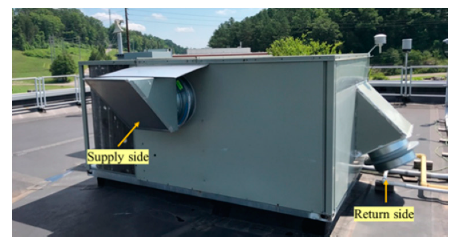
The flexible research platform (FRP) in Oak Ridge National Lab (ORNL) was used for the RTU experiment (Figure 1). It is a common two-story lightweight commercial building consisting of slabs and a steel superstructure with a footprint of 13.4 m by 13.4 m. A 44-kW RTU with a DX cooling coil system conditions zones of the building with an air handling unit (AHU) and VAV boxes in each room, as shown in Figure 1 (right). The DX cooling system consists of two cooling coils that operate with two stages. One cooling coil turns on in stage 1, and two coils are on in stage 2. Stage 2 is triggered when the supply air temperature is not maintained at the setpoint (e.g., 12.8 °C (55 °F)).
2.2. RTU Modeling
2.2.1. General RTU Model Structure
In general, the power consumption of a DX cooling coil consists of multiple polynomials regarding the cooling capacity, energy input ratio (EIR), and part load ratio (PLR). They are functions of the outdoor air temperature and air temperature passing the cooling coil. The latter is a wet-bulb temperature, which can be calculated based on the air temperature and relative humidity. Each polynomial does not vary dramatically from one, and they are multiplied by the nominal value (i.e., rated condition), so they do not deviate much from the nominal performance. In this study, a general form is adopted from the EnergyPlus engineering reference (Equation (1)) [27].
where:
2.2.2. Modeling Results
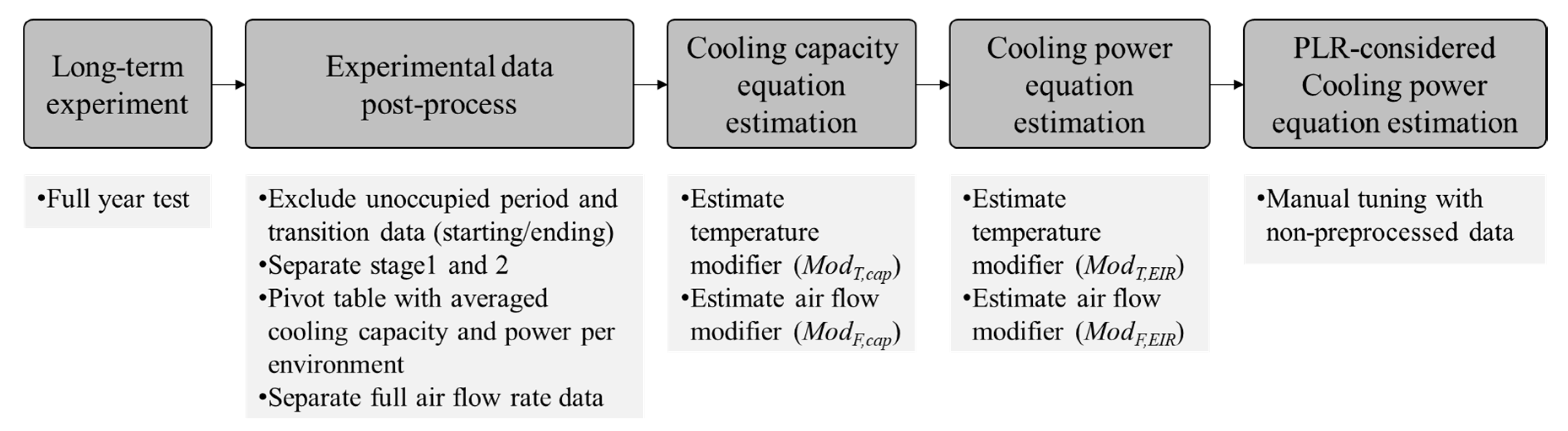
Figure 2 presents the process to obtain the RTU model from the experiments. The process includes (1) a long-term experiment (e.g., a full year), (2) post-processing to obtain steady-state experimental data, (3) cooling capacity curve estimation, (4) EIR curve estimation, and (5) PLR curve estimation.
The RTU was operated constantly for a year (2017) according to the test procedure for multiple research projects. The setpoint temperature of the supply air was set to 12.8 °C (55 °F) and 16.7 °C (62 °F) for cooling and heating seasons with binary control (on/off) of the two cooling coils. The second cooling coil is only activated when the supply air temperature is not maintained at the setpoint. The supply fan is operated according to the duct pressure with VAV damper operation. During the test, the temperature and humidity of the supply and return air, the outdoor air temperature, the air flow rate through the RTU, and the power consumption of the RTU are measured.
To create the performance curve, quasi-steady-state data were filtered from 1 year of HVAC operation data (6 a.m.–6 p.m. for cooling season and 7 a.m.–10 p.m. for heating season) with 1-min resolution (268,778 data points). The transition period was excluded for the starting/ending times (6- and 4-min data points, respectively). The number of the final data points is 41,457. Then pivot tables were built in an Excel sheet to provide the averaged cooling capacity and power consumption of the RTU with respect to Tout and Tcoil for each stage. The sizes of the pivot tables are 1653 and 344 for stages 1 and 2, respectively. Finally, the data of the full air flow rate were separated.
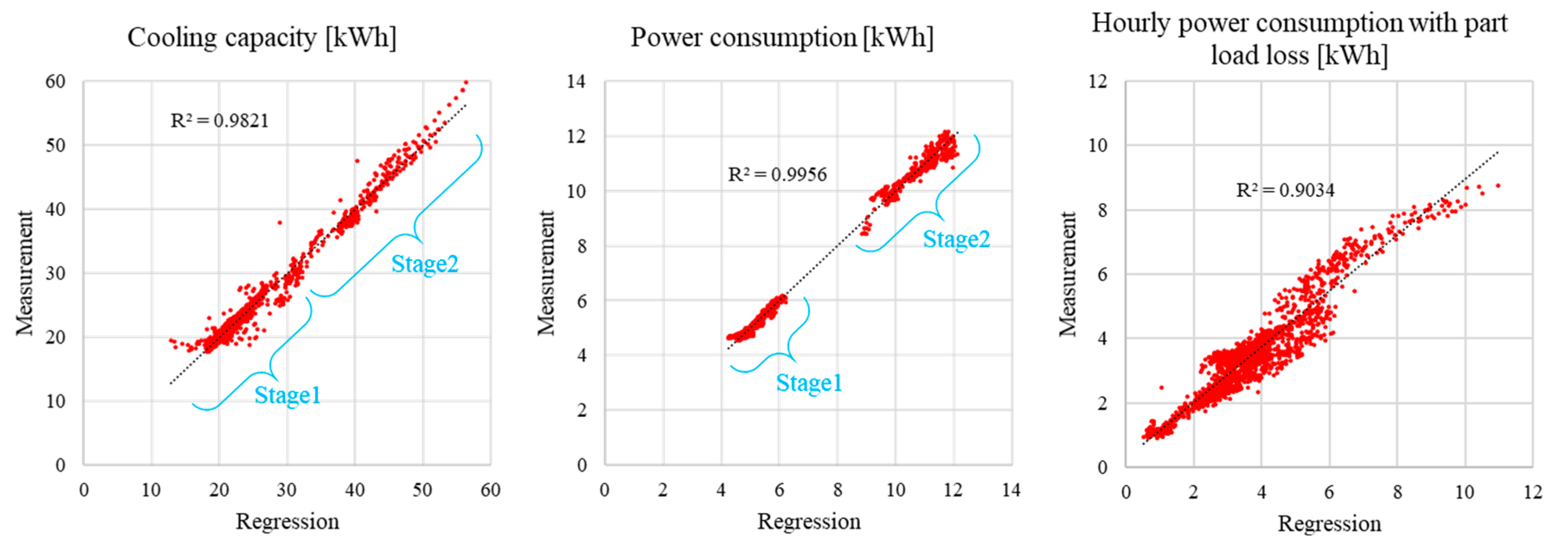
Gross cooling capacity was calculated with the enthalpy difference between the mixed and supply air across the RTU using temperature/humidity sensors installed in the RTU, as shown in Figure 1 (bottom), which is based on ASHRAE fundamental [28]. Then the coefficients of the temperature modifier for the cooling capacity (Ccap,i (i = 1–6)) were estimated with full air flow rate data. Constrained linear regression was carried out in Matlab (lsqlin). The inequality constraint was set to normalize the multiplier so that it is close to one in rated conditions (67 °F and 95 °F for Tout and TWB,coil). Then the coefficients of the air flow rate modifier (Ccap,i (i = 7–9)) were estimated in the same fashion with varying air flow data.
Figure 3 (left) shows the result of the regression for the cooling capacity. The horizontal and vertical axes represent the regressed and experimental value. The root mean square error (RMSE) of the model compared to the experimental data is 0.96 kWh, and its correlation coefficient (R2) is 0.98. The coefficients for EIR (CEIR,i (i = 1–9)) were estimated in the same fashion. Figure 3 (center) shows the result of the regression for the power consumption. The RMSE and correlation coefficient are 0.14 kWh and 0.99, respectively.
Previous sections focused on estimating the coefficient for the cooling capacity and EIR without the loss from the PLR, so the data was filtered to only consider the ideal cases without the loss from the part load operation. In this section, however, unfiltered data (268,778) are used with 1-min resolution. These 1-min data are averaged for an hour to capture the average power loss of the on/off operation of the RTU. Typical coefficients for PLR are 0.85 and 0.15. Manual calibration with 2-digit resolution yields the best results at 0.8 and 0.2. Figure 3 (right) shows the regression results of the hourly power consumption considering the loss from the PLR. The RMSE and correlation coefficient are 0.39 kWh and 0.99, respectively. The final coefficients are summarized in Table 1.
2.2.3. Model Analysis
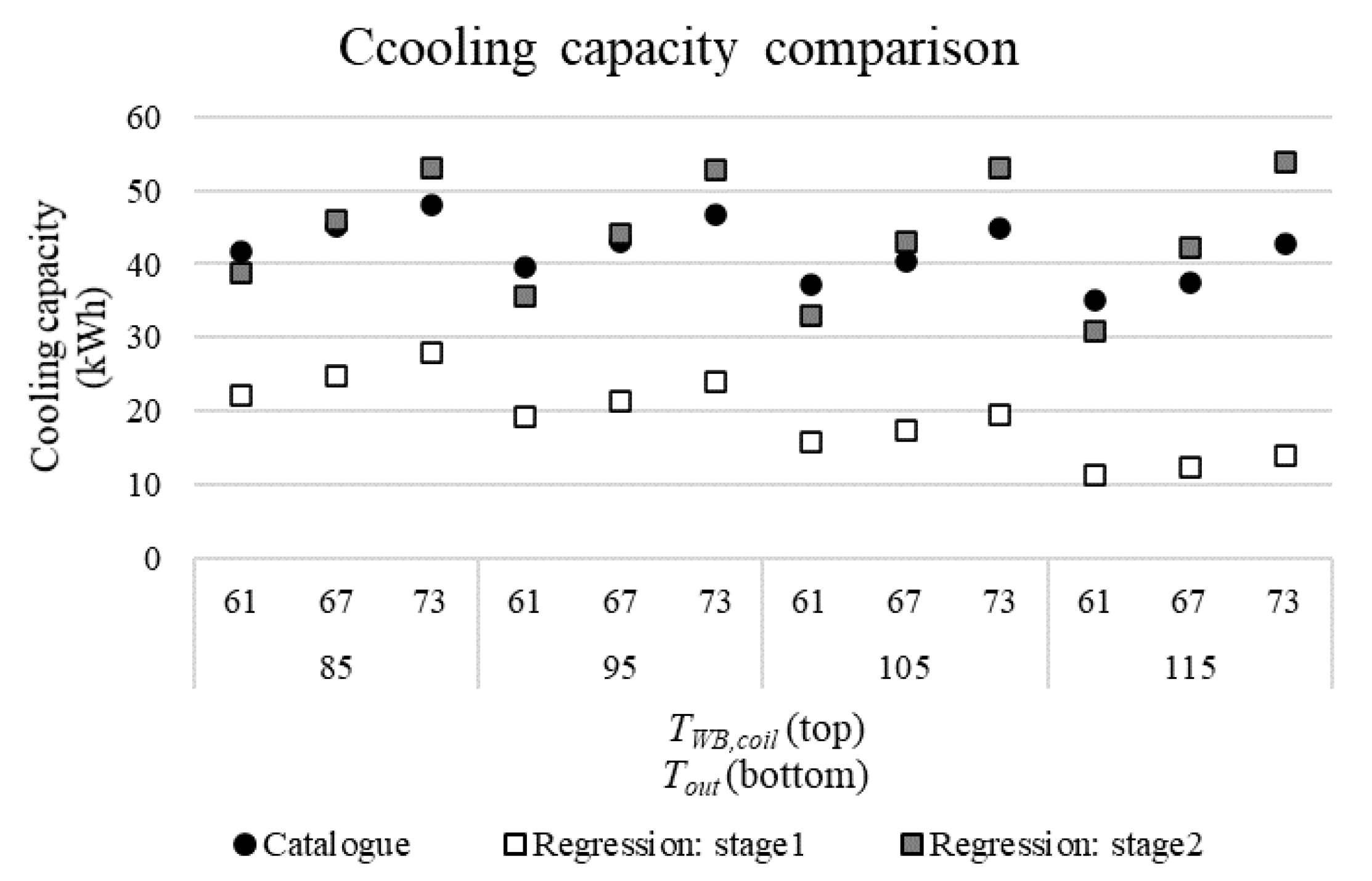
The performance of the estimated RTU model was compared with that of the manufacturer’s data (Figure 4). We assume that the performance data with gross cooling capacity in the manufacturer are based on stage 2 operation. According to the comparison, regression with stage 2 operation is close to the manufacturer data. Unfortunately, no cooling power data are provided from the manufacturer. Even though the manufacturer data follow the performance trend of the actual measurement, they are limited as only stage 2 operation is provided, and cooling power performance is not given.
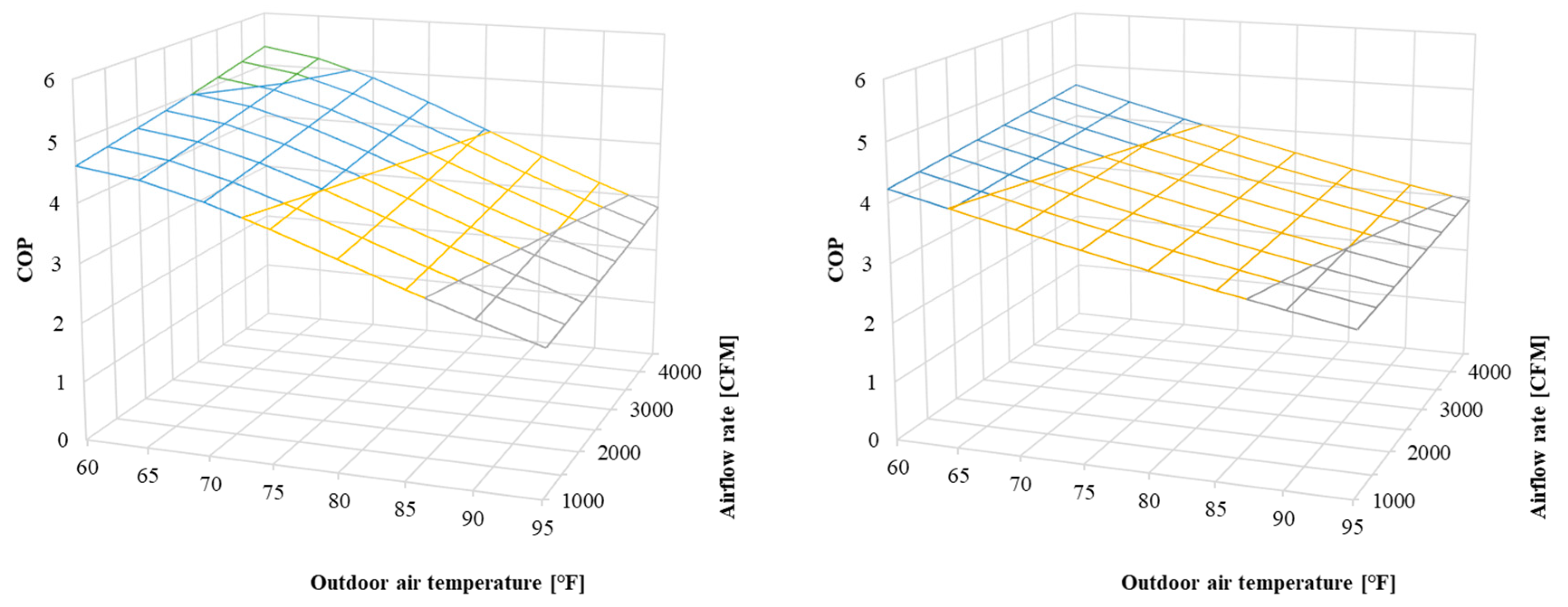
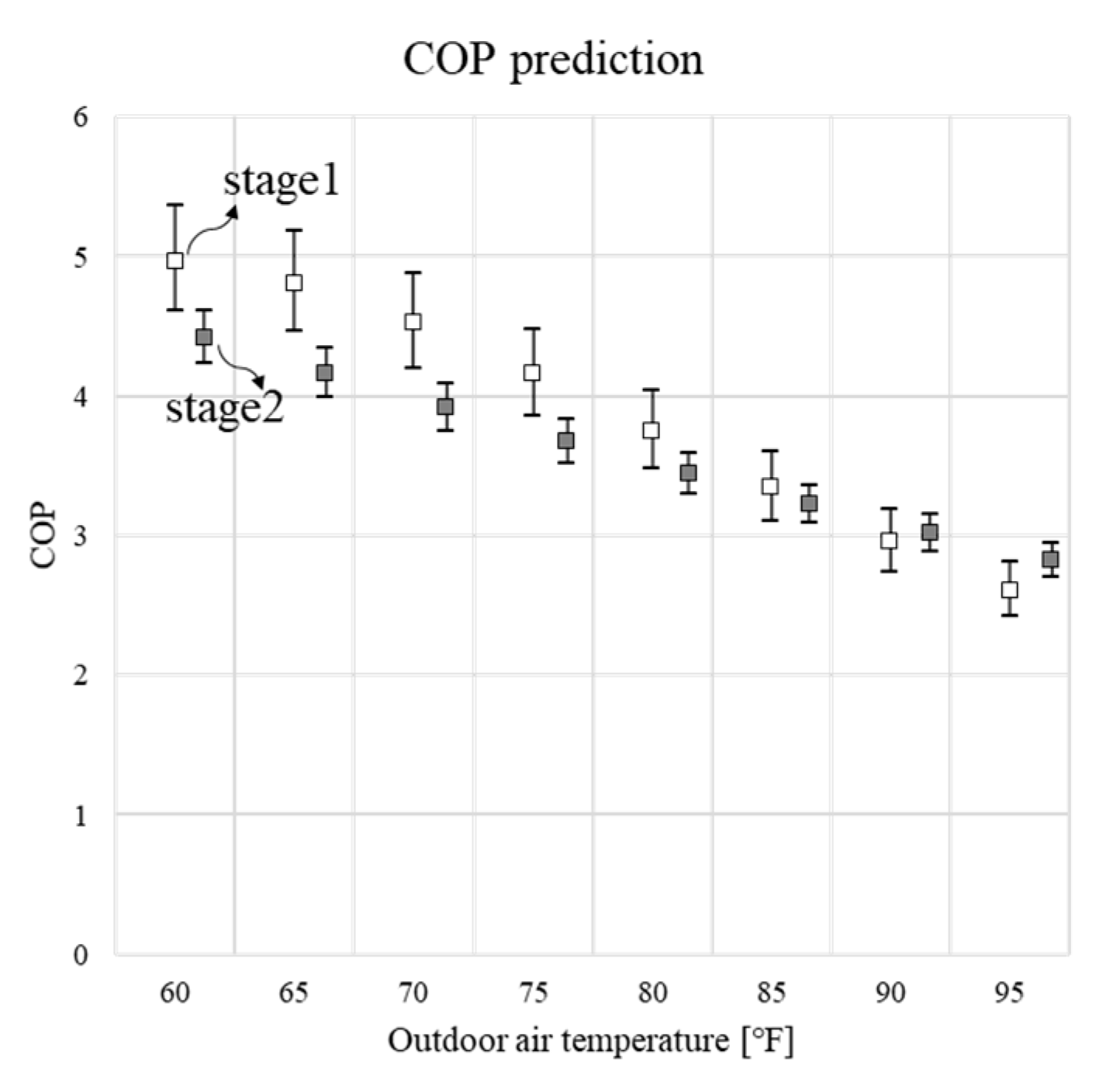
Figure 5 shows the COP variation of the estimated RTU model with respect to the outdoor air temperature and airflow rate. The wetbulb temperature of the air entering the cooling coil (TWB,coil) is fixed at 67 °F (19.4 °C). The left and right figures show stage 1 and stage 2, respectively. As one can expect, the COP becomes high when the outdoor air temperature is low. Likewise, the higher COP is obtained with higher airflow. However, this is not as sensitive as the impact from the outdoor air temperature. The experimental data for the stage 1 are obtained when the outdoor air temperature is not that high and vice versa for the stage 2 which is activated only for hot weather condition. Ideally, those two could be united to one curve by dividing the weather/operation condition between two stages. Figure 6 presents the simplified relation between the COP and outdoor air temperature. It shows the maximum, average, and minimum value from the airflow rate variation for stages 1 and 2 with TWB,coil fixed at 67 °F (19.4 °C). Typically, stage 2 is required when the outdoor air temperature is high, so stage 2 data might not be applicable with lower outdoor air temperature.
3. Case Study
In this section, simulation/experimental case studies were carried out with regressed RTU model to evaluate the significance of the model in three different research topics. In building energy modeling study (Case 1), cooling DX electricity consumption, delivered cooling energy, and room air temperature were compared between the simulation and experiment. In MPC study (Case 2), the room air temperatures were compared between the simulation and experiment for the building modeling. Then the cooling rate, power consumption, and corresponding electricity cost of the simulations with different control strategies were compared. In the FDD study (Case 3), the COP, delivered cooling, and power consumption were compared between the simulated performance with regressed RTU model and experimental test based on the faults that were implemented by the authors.
3.1. Case 1: Building Energy Modeling Study
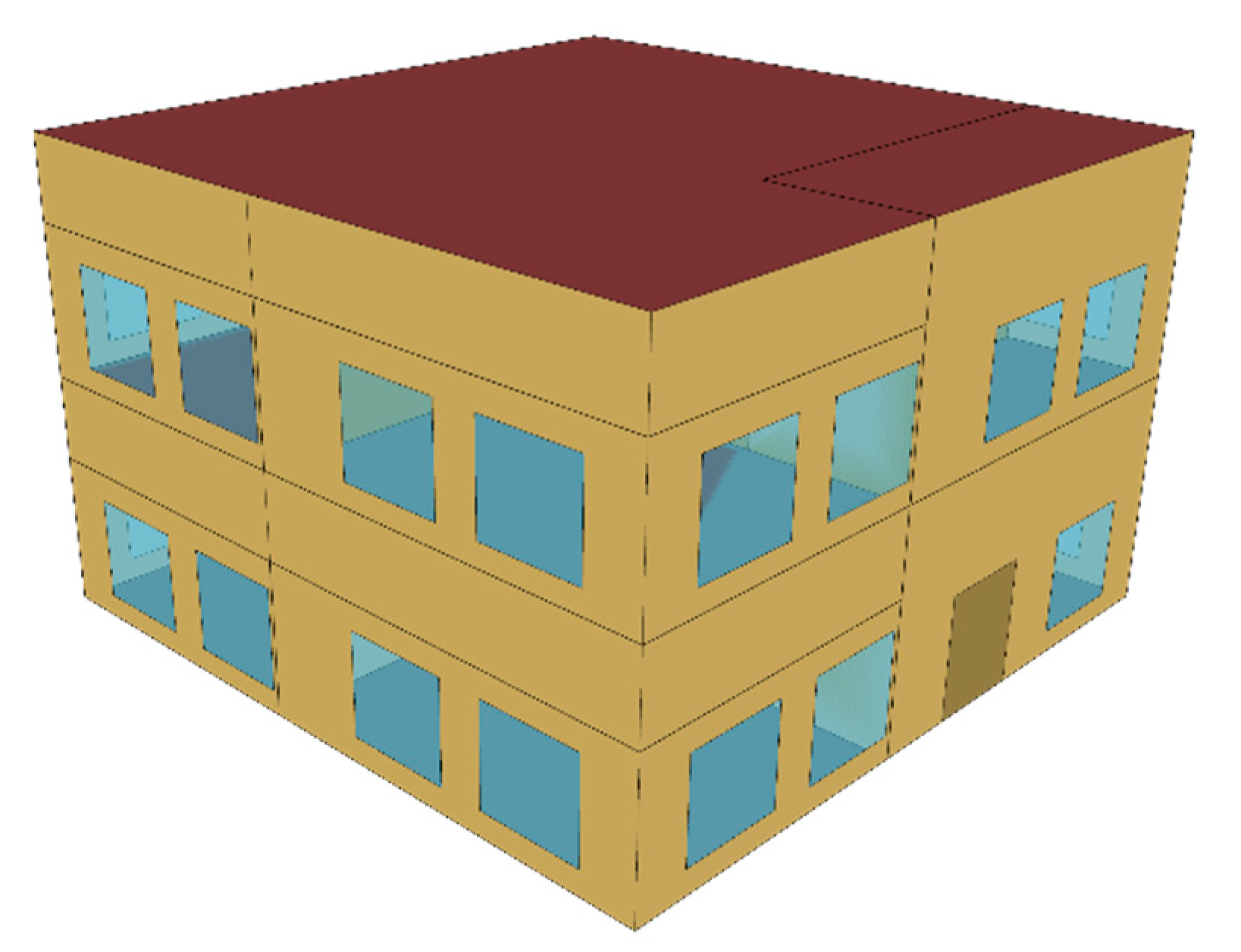
The regressed RTU model in previous section was tested in a building energy modeling study with a simulation program, EnergyPlus. The building envelope model was constructed in OpenStudio according to the building information from drawings, specifications, and a site audit (Figure 7). Then the model was imported in the EnergyPlus program for the additional settings of the HVAC system and envelope details. The weather file was packed based on the data from the weather station on the roof. In addition, a blower door and tracer gas test were performed to identify the infiltration rate of the building envelope and input to the simulation.
The AHU and VAV were modeled with ZoneHVAC:OutdoorAirUnit and AirTerminal:SingleDuct:VAV:Reheat. The RTU DX cooling system was modeled with Coil:Cooling:DX:TwoStageWithHumidityControlMode. The regressed cooling coil performance was implemented with Curve:Quadratic and Curve:Biquadratic, while the detailed performance information, such as the COP and cooling capacity, was input in CoilPerformance:DX:Cooling.
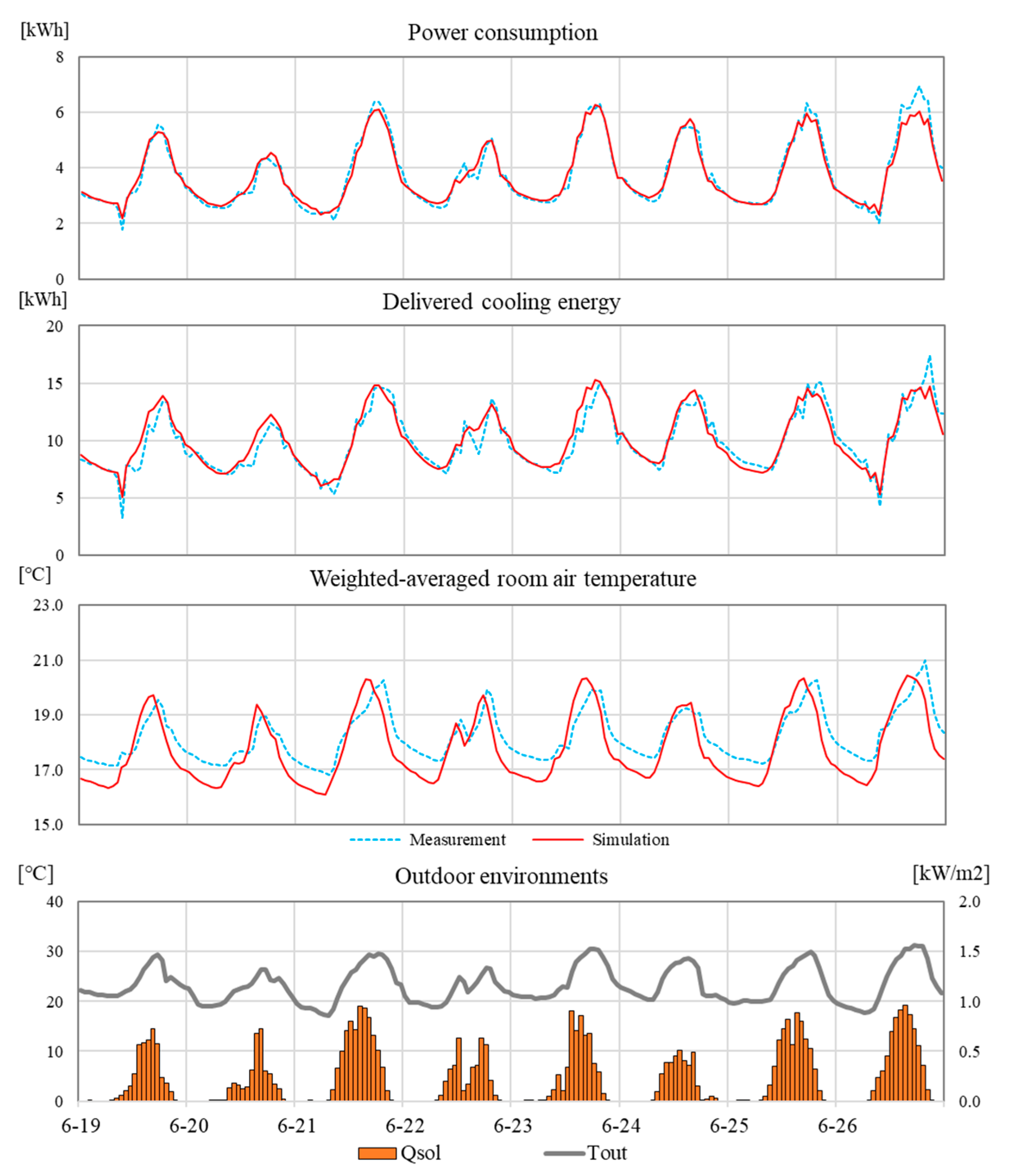
The experiment for the validation test was performed for 8 days in the cooling season (19–26 June 2019). A total of 10 zones were conditioned with a fixed damper position at a minimum opening rate and providing air flow from 116 to 352 cfm (cubic feet per minute). The setpoint of the supply air temperature from the AHU was set to 12.8 °C (55 °F), and measurements show fluctuation of approximately ±1.5 °C due to the on/off control of the RTU. During the test, all heating coils in the AHU and VAV were turned off. The room air setpoint temperature of all zones was set to 22.2 °C (69.8 °F). However, they were not maintained at the setpoint due to the minimum airflow rate with the fixed damper position, and the reheating coils were not operated. The detailed procedure and grounds for the experiment are described in a previous study [13].
Figure 8 shows the validation results along with environmental data. The simulated RTU cooling power consumption and delivered cooling matched well with the experimental trajectories. The simulation trajectory of the average (volume-weight) room air temperature follows the trend of the experimental trajectory. However, it was impossible to match all trajectories of the room air temperatures (not shown in the figure due to the page limit), which vary according to characteristics such as the room size, window orientation, and window-wall ratio.
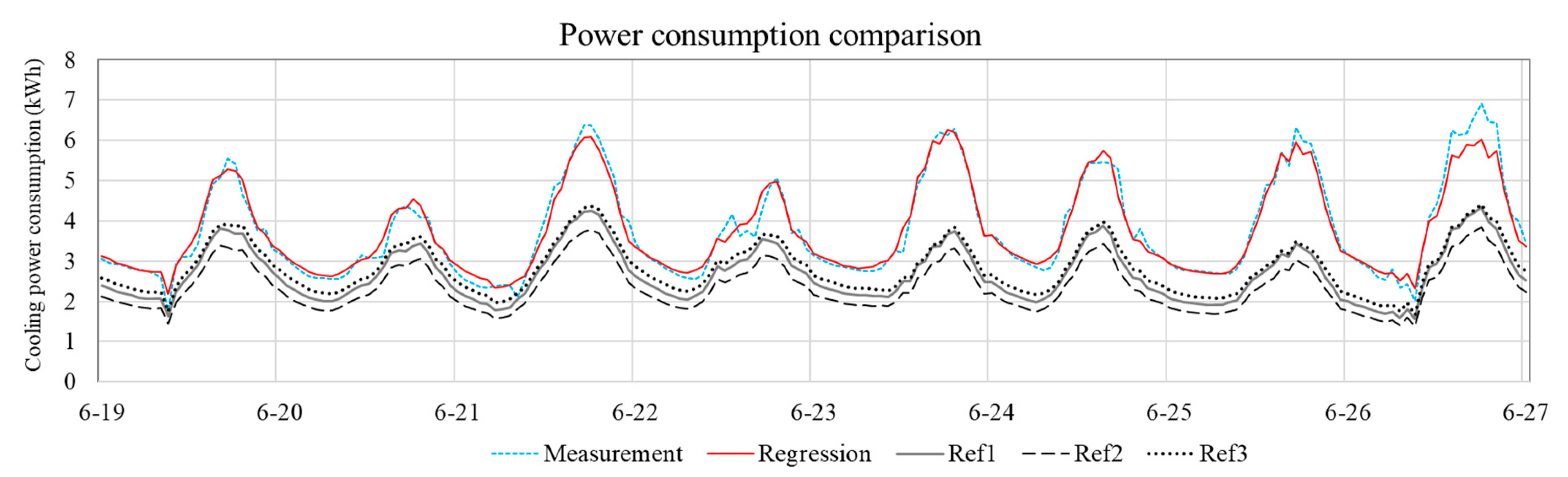
The regressed RTU model was compared with the generic models in the open dataset of EnergyPlus. Three curves (Lennox KCA120S4, Lennox SCA120H4B, Lennox TCA120S) that are operated with similar cooling capacity were selected. Only the curve data (Curve:Quadratic, Curve:Biquadratic) are used, while the coil performance remains the same (CoilPerformance:DX:Cooling). Figure 9 shows the comparison of the measured and simulated cooling power trajectories and reference curves. The NMBE and coefficient of variation of sRMSE (cv(RMSE)) obtained with the naive adoption of the nominal curve are −21.7~−37.1% and 25.5–41.4%, but those of the regressed curve are reduced to −0.2% and 6.1%, respectively.
3.2. Case 2: Model-Based Predictive Control (MPC)
The second case was an MPC study. A control-oriented building model was estimated with actual building operation data and then input to a state-space formulation for optimization in MPC. The grey-box model structure was applied, which is simple and robust so has been applied for a number of MPC studies [29,30]. The experiment was conducted for four days (21–24 September 2019) to generate building data from the test-bed. A total of 10 zones of the FRP were conditioned with bang-bang control to decorrelate the impact of the control and disturbance inputs to the output. This was done to facilitate the estimation process and obtain a robust building model.
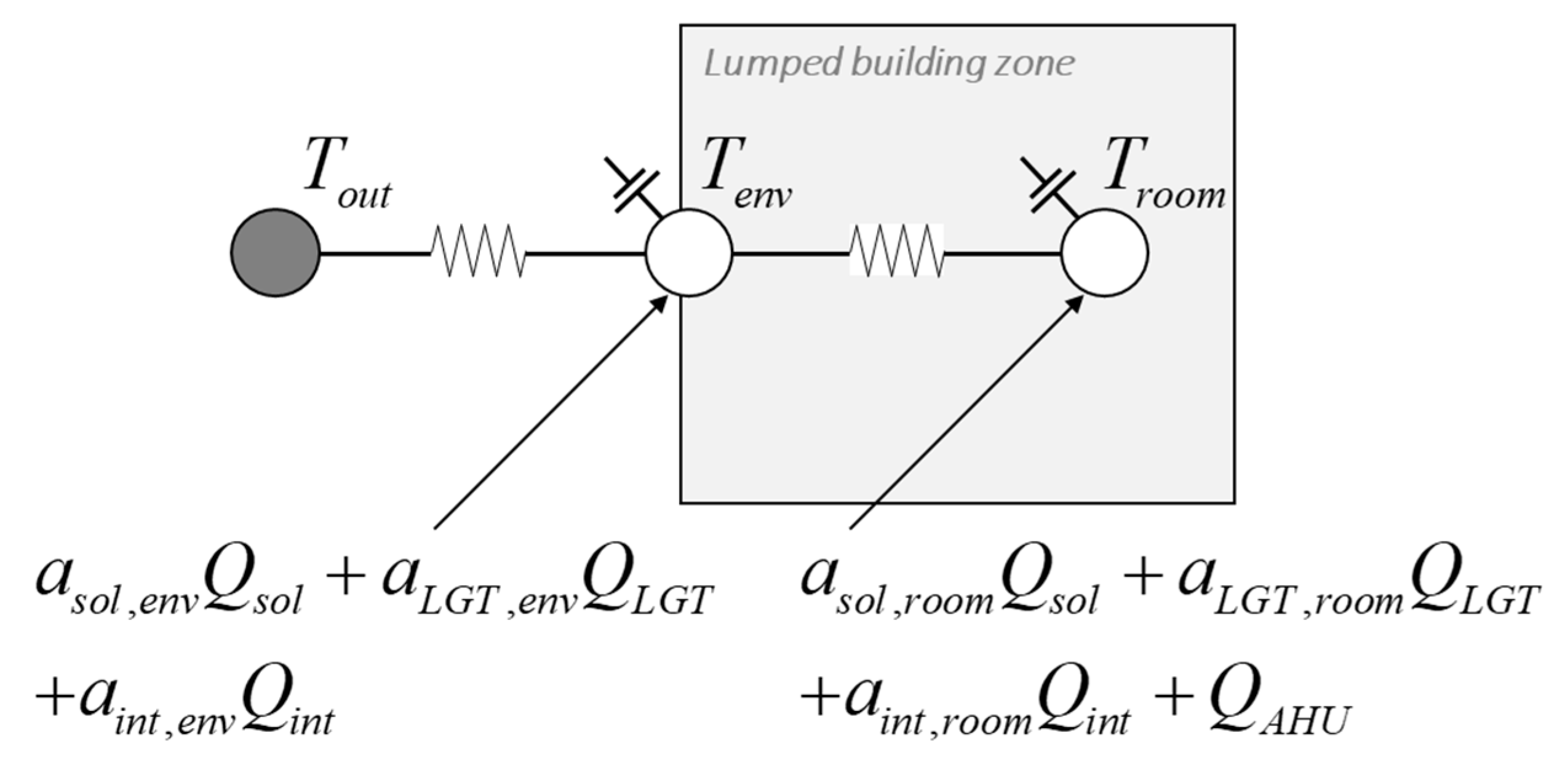
To simplify the building model, the 10 building zones were lumped into a single-zone model, as shown in Figure 10. This is the 2C2R model with one boundary temperature (Tout), one control input (QAHU), and three disturbance inputs (Qsol, QLGT, and Qint). The cooling rate from the supply duct to each zone and the internal heat gain are summed and input to each state (envelope and room node). The heat gain from the lighting (QLGT) and internal equipment (a heater in this study, Qint) are distributed to the envelope and room nodes; αLGT,room + αLGT,env = 1 and αint,room + αint,env = 1. The corresponding state-space formulations are shown in Equations (2) and (3).
where:
Non-linear optimization was performed to identify the model parameters (Roe, Rer, Cenv, Croom, αsol,env, and αsol,room) with the average (volume-weight) room air temperature. The internal Matlab function fmincon was used. The initial values of the estimate parameters, such as the convective heat transfer coefficient, were adopted from the building energy simulation program. Figure 11 presents the estimation and validation results along with the control and disturbance inputs. The RMSE of the estimated building model was 0.76 °C, which is acceptable for implementation in the simulation and actual test-bed building.
The MPC simulation was performed with the estimated building and RTU models. In the MPC formulation, a simple COP prediction with linear relation to the outdoor air temperature was used, as shown in Equation (4). This was derived from Figure 6 based on the least squares method. All stage 1 data were used, while only high-temperature data (80–95 °F) were applied.
To formulate the linear optimization (e.g., linear programming), the continuous state space formulation was discretized with a time step k, and then the input matrix B was divided according to the disturbance and control input (Equations (5) and (6)). Bd,w and Bd,Q are input matrices incorporating the disturbance and control input. This was iterated with the time step, and a series of matrices were generated, including a column matrix (Ωx) and lower triangular matrices (Ωw and Ωu), as shown in Equation (7). The matrices are expressed with bold notation.
Equation (8) represents the optimization formulation for the MPC simulation. The objective function is the electricity consumption of the RTU, which is calculated by dividing the control input matrix (QAHU) by the predicted COP (COPT, where T is the transpose operator). The room air temperatures (Tlower and Tupper) are set to 20 °C and 23 °C. They are hard constraints incorporated in an inequality constraint so that no comfort violation occurs in the room during the optimization. CT is a pre-defined matrix for extracting the target temperature from the state (e.g., air temperature).
where:
The existing Matlab solver linprog was used for solving the linear programming problem. The time step and the prediction horizon were set to 15 min and 24 h, so the dimension of the control input (QAHU) is 96. The initial state temperatures for the envelope and room were set to 21.5 °C, which is the mid-point of the comfort bound. Ventilation load is not considered (i.e., no outdoor air is included in the cooling load calculation).
One-day data after the estimation/validation period were selected (25 September 2019), which was a typical sunny day in the cooling season (the maximum and minimum outdoor air temperatures were 32.7 °C and 12.2 °C). One-shot optimization was carried out with measured disturbances including weather data (outdoor air temperature and solar radiation) and internal heat gain profiles. The estimated RTU model was incorporated after calculating the MPC with the simplified COP prediction. A typical feedback controller was simulated with the estimated building model to evaluate the MPC performance.
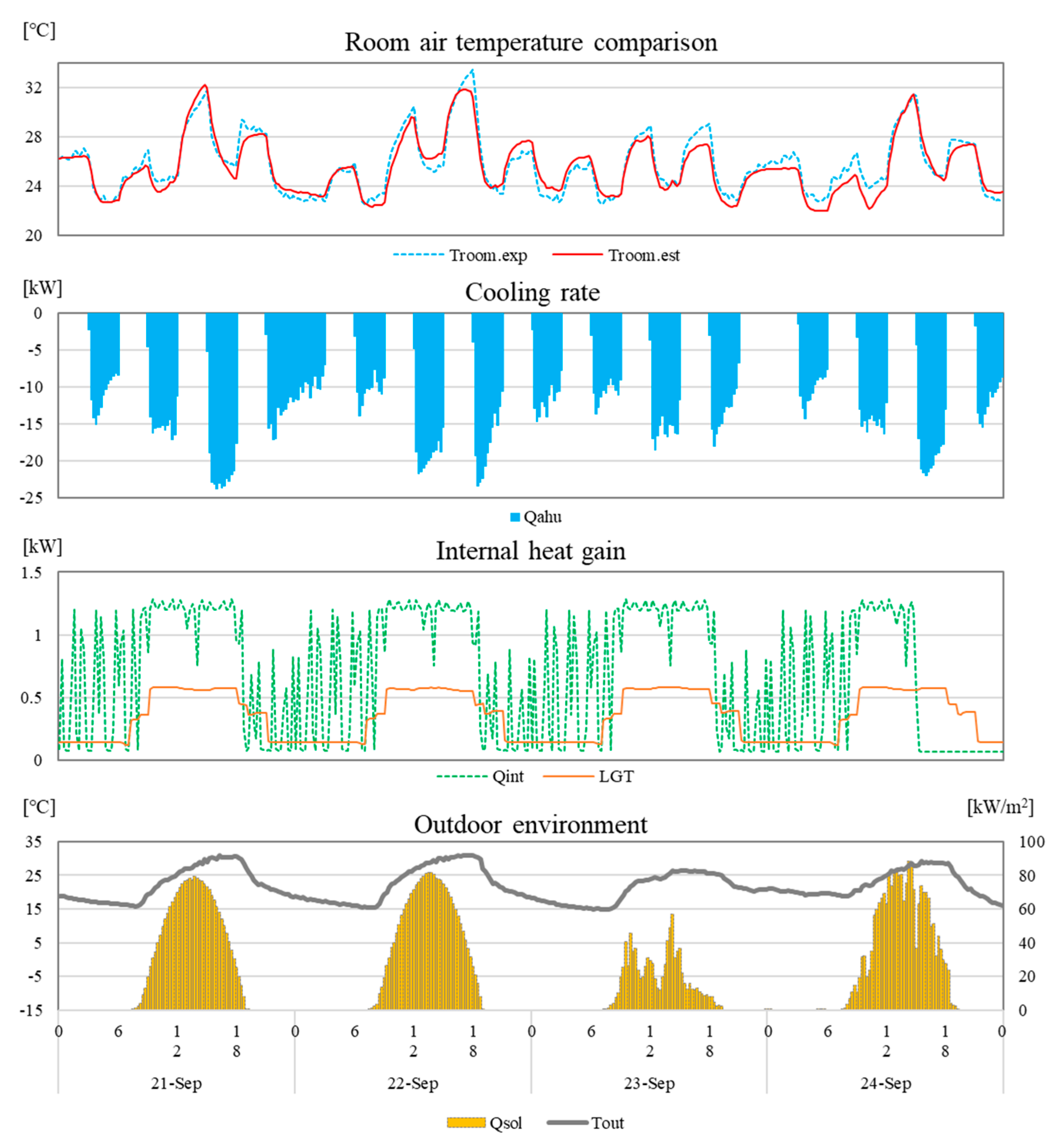
Figure 12 shows the performance comparison of the MPC and feedback control. It shows the room air temperature, cooling rate, power consumption of the RTU (regressed model in Section 2), and disturbances, including solar radiation and outdoor air temperature. The cooling rate was input to the zone when the outdoor air temperature was low and the corresponding COP was high (e.g., 2 a.m. to 5 a.m.) in the MPC. The amount of power consumption of the pre-cooling was relatively low due to the higher COP at night. The relative savings potential of the MPC in the power consumption is 14.4% compared to the feedback control. The cost saving is 12.5% when the typical electricity cost at the time of use (TOU) was applied; we assumed that the peak price is twice the off-peak price, and their average is 12.7 ¢/kWh which is approximately the nation-wide average [31]. The cost saving can be increased when a more aggressive TOU policy is applied. The results are summarized in Table 2.
3.3. Case3: Fault Diagnostics and Detection (FDD)
An FDD study was conducted in a third case study using the regressed RTU model. Three main fault conditions were identified in terms of the RTU operation: duct leakage, limited refrigerant, and condenser fouling. They are ranked as the 2nd, 4th, and 7th most common faults in the top 20 faults that occur in small commercial buildings in the U.S. [22]. This is a purely experiment-based study and was carried out for several days in two years (2017–2018). All tests were done with a typical occupancy schedule (e.g., 07 a.m. to 10 p.m.) using heaters, humidifiers, and lighting on the ceiling without actual occupants. The setpoint temperature of all rooms was set to 23.9 °C (75 °F). The detailed information regarding the experiments was described in a previous study [26].
To generate the leakage in current RTU while not damaging the actual systems (e.g., cooling/heating coils, chiller, fan, etc.) from rain and other incidents, cylinder-type iris dampers (Fantech IR16 Iris Damper) were installed on the supply and return sides (the economizer specifically), as shown in Figure 13. They enable manual control of the level of the air leakage from outside. Only the damper in the return side was activated.
There is no direct measurement for the return duct leakage rate. The air flow can be determined from the K factor and differential pressure measurements. The lever in the damper can be adjusted to select the K factor. The equation to estimate the airflow is:
where q is the airflow rate in cfm, and ∆p is the differential pressure in w.c. Different levels of return duct rates were tested by adjusting the K value and measuring ∆p. The test results show that around 12% and 23% return duct leakage can be achieved with K values of 1500 and 6750, respectively. As the maximum value of K is 6750, higher return duct leakage was not tested. Based on this preliminary test, leakage tests with 12% and 23% were carried out.
“Limited refrigerant” refers to operating the RTU with an inappropriate or smaller amount of refrigerant. This fault can occur due to human error or mechanical issues such as leaking. This damages the performance of the compression cycle of the RTU, so the cooling capacity and efficiency are degraded. To emulate this fault, we manually injected less refrigerant (70%) in the pipe line.
Condenser fouling refers to decreasing the airflow rate across the condenser fan due to dust, dirt, or litter on the condenser unit’s fins. This fouling degrades the heat transfer rate between the refrigerant in the condenser unit and the air induced by the condenser fan. To emulate this fault without damaging the facility, two different levels of porous fabrics were applied on the external surface of the condenser, as shown in Figure 14. Air reductions of 28% and 58% were achieved compared to the case without the fabric according to manual measurement with a hand-held airflow meter.
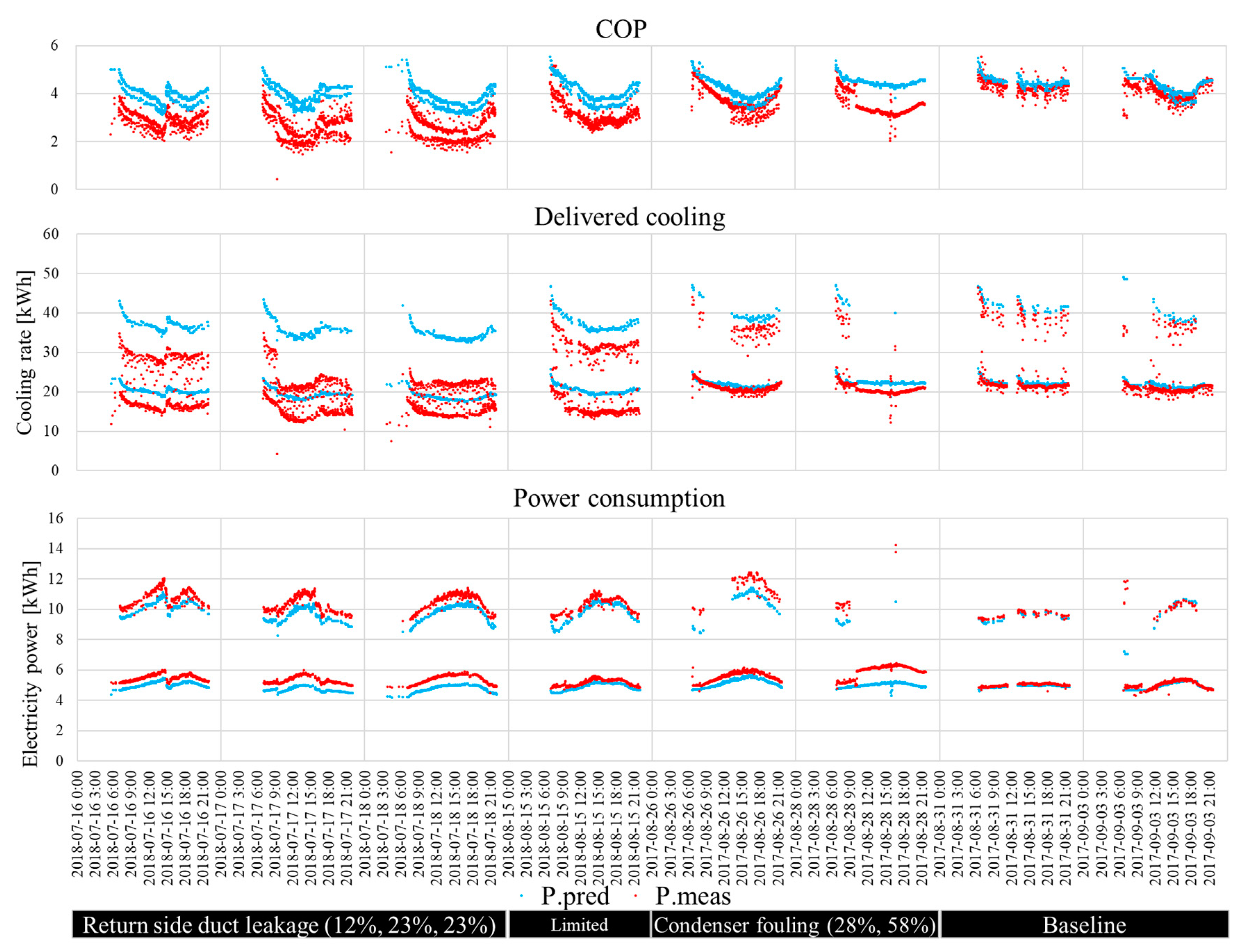
Figure 15 shows the results of the three fault tests along with the baseline case. The COP, delivered cooling, and RTU’s total power consumption are shown with 1-min resolution. Transition data for turning on the RTU and between stages were deleted as a bias to evaluate the prediction performance of the model. The error metric was evaluated with the daily cv(RMSE) in percentage (%) and is summarized in Figure 16. As one can see, the prediction with the estimated model and experimental data matched well at baseline. However, in all cases, the power consumption does not deviate as much as the COP and delivered cooling. It can be concluded that the fault should not be evaluated with only power consumption prediction but also with the delivered cooling prediction or COP, which is calculated based on the delivered cooling.
When the outdoor air is infiltrated through the RTU return side (i.e., return duct leakage), the delivered cooling measurement was reduced to 22–32%, while the power consumption increased slightly compared to the prediction based on the model. This makes sense according to the sensing point of the return air. The actual return air sensor is located typically before the mixing box and unintentionally mixed with infiltrating outdoor air. The cv(RMSE) between the measurement and prediction is 31–55%. The more duct leakage is produced, the less delivered cooling is produced (e.g., compare the leakage rates of 12% and 23%). This trend is seen in the power consumption—more power consumption is required for a higher leakage rate. However, the deviation is not distinct compared to the delivered cooling case.
As for the limited refrigerant case, it does not affect the power consumption distinctively, but the delivered cooling decreases about 19%. When the heat exchange rate in the condenser side degrades (i.e., condenser fouling), distinct deviation between the prediction and measurement is not seen. The more fouling occurs (e.g., compare the airflow reduction rates of 28% and 58%), the less delivered cooling is produced, and more power is required.
4. Conclusions and Discussion
This study presented a general procedure to generate a DX cooling coil system for an RTU and evaluated the applicability of the model to multiple cases. Regression was carried out with experimental data for predicting the cooling capacity and power consumption. Based on the estimated model, three case studies were carried out.
- The estimated DX cooling model for RTU system matched well with the measurement for the two stages. Their RMSE and correlation coefficient were 0.96kW and 0.98 in the cooling capacity and 0.14kW and 0.99 in power consumption.
- A BES program validation with EnergyPlus was conducted with a 2-story unoccupied commercial building. The power consumption of the model matched well with the experiment compared to the naive adoption of the nominal curve. The NMBE and cv(RMSE) improved from −21.7~−37.1% and 25.5~41.4% to −0.2% and 6.1%, respectively.
- An MPC simulation study was carried out with an estimated grey-box building and RTU models. Simplified linear COP prediction was incorporated in the MPC formulation, and 14.3% power savings was achieved compared to the feedback control.
- Three fault tests (duct leakage, limited refrigerant, and condenser fouling) were performed with the regressed RTU model. In all cases, the delivered cooling decreased distinctively. The cv(RMSE) of faulty experimental data against the model was 7~52% while the normal experimental data against the model were 9% (baseline). However, the power consumption of the faulty condition increased slightly compared to the prediction from the model.
The scope of this study was limited to quick case studies to evaluate the applicability of the RTU model. Empirical validation was only carried out with a single tool (EnergyPlus), and the analysis of the building envelope to match the indoor air temperature was not fully investigated. The MPC simulation study was carried out for one day with a simplified/lumped (single) zone from a multi-zone building. In the FDD study, a detailed algorithm to predict the fault was not discussed, and only a simple error metric (cv(RMSE)) with trajectories in figures was presented. Further evaluation with a detailed analysis for each case study can be performed in future work.
Author Contributions
Manuscript writing: J.J. and P.I.; data analysis, modeling, validation, and simulations: J.J., P.I., and J.D.; supervision, project administration, funding acquisition: P.I.; experiment: J.J., and P.I.; All authors have read and agreed to the published version of the manuscript.
Funding
This material is based upon work supported by DOE’s Office of Science and BTO. This research used resources of ORNL’s Building Technologies Research and Integration (BTRIC), which is a DOE Office of Science User Facility. This work was supported by INHA UNIVERSITY Research Grant.
Acknowledgments
This manuscript has been authored by UT-Battelle, LLC, under Contract No. DE-AC05-00OR22725 with the U.S. Department of Energy. The United States Government retains and the publisher, by accepting the article for publication, acknowledges that the United States Government retains a non-exclusive, paid-up, irrevocable, worldwide license to publish or reproduce the published form of this manuscript, or allow others to do so, for United States Government purposes. The Department of Energy will provide public access to these results of federally sponsored research in accordance with the DOE Public Access Plan (http://energy.gov/downloads/doe-public-access-plan).
Conflicts of Interest
The authors declare no conflict of interest.
References
- Department of Energy (DOE)—Commercial Building Energy Alliances (CBEA). 2012. Available online: https://www1.eere.energy.gov/buildings/alliances/rooftop_specification.html (accessed on 15 January 2020).
- Feng, K.; Lu, W.; Wang, Y. Assessing environmental performance in early building design stage: An integrated parametric design and machine learning method. Sustain. Cities Soc. 2019, 50, 101596. [Google Scholar] [CrossRef]
- Wang, R.; Lu, S.; Li, Q. Multi-criteria comprehensive study on predictive algorithm of hourly heating energy consumption for residential buildings. Sustain. Cities Soc. 2019, 49, 101623. [Google Scholar] [CrossRef]
- Seyedzadeh, S.; Pour Rahimian, F.; Rastogi, P.; Glesk, I. Tuning machine learning models for prediction of building energy loads. Sustain. Cities Soc. 2019, 47, 101484. [Google Scholar] [CrossRef]
- Moreci, E.; Ciulla, G.; Brano, V.L. Annual heating energy requirements of office buildings in a European climate. Sustain. Cities Soc. 2016, 20, 81–95. [Google Scholar] [CrossRef]
- Ascione, F.; Bianco, N.; De Stasio, C.; Mauro, G.M.; Vanoli, G.P. A New Comprehensive Approach for Cost-Optimal Building Design Integrated with the Multi-Objective Model Predictive Control of HVAC Systems. Sustain. Cities Soc. 2017, 31, 136–150. [Google Scholar] [CrossRef]
- Péan, T.; Costa-Castelló, R.; Salom, J. Price and Carbon-Based Energy Flexibility of Residential Heating and Cooling Loads Using Model Predictive Control. Sustain. Cities Soc. 2019, 50, 101579. [Google Scholar] [CrossRef]
- Fang, J.; Ma, R.; Deng, Y. Identification of the Optimal Control Strategies for the Energy-Efficient Ventilation under the Model Predictive Control. Sustain. Cities Soc. 2020, 53, 101908. [Google Scholar] [CrossRef]
- Du, Z.; Fan, B.; Jin, X.; Chi, J. Fault detection and diagnosis for buildings and HVAC systems using combined neural networks and subtractive clustering analysis. Build. Environ. 2014, 73, 1–11. [Google Scholar] [CrossRef]
- Li, S.; Wen, J. A model-based fault detection and diagnostic methodology based on PCA method and wavelet transform. Energy Build. 2014, 68, 63–71. [Google Scholar] [CrossRef]
- Gorthala, R. Bringing Fault Detection and Diagnosis (FDD) Tools into the Mainstream: Retro Commissioning & Continuous Commissioning of HVAC and Refrigeration Systems. BTO peer review 2017. Available online: https://www.energy.gov/sites/prod/files/2019/05/f62/bto-peer%E2%80%932019-univ-new-haven.pdf (accessed on 21 October 2020).
- Consortium for Building Energy Innovation (CBEI), 2016, OpenStudio Measure Development for Integrated HVAC Retrofit. Available online: http://www.cbei.psu.edu/wp-content/uploads/2016/07/OpenStudio-Measure-Development-for-Integrated-HVAC-Retrofit.pdf (accessed on 21 October 2020).
- Im, P.; Joe, J.; New, R.J.; Bae, Y. Empirical Validation of Building Energy Modeling for Multi-zones Commercial Buildings in Cooling Season. Appl. Energy 2020, 261, 114374. [Google Scholar] [CrossRef]
- Im, P.; New, R.J.; Joe, J. Empirical Validation of Building Energy Modeling using Flexible Research Platform. In Proceedings of the 16th IBPSA International Conference, Rome, Italy, 2–4 September 2019. [Google Scholar]
- Oldewurtel, F.; Parisio, A.; Jones, C.N.; Gyalistras, D.; Gwerder, M.; Stauch, V.; Lehmann, B.; Morari, M. Use of Model Predictive Control and Weather Forecasts for Energy Efficient Building Climate Control. Energy Build. 2012, 45, 15–27. [Google Scholar] [CrossRef] [Green Version]
- Joe, J.; Karava, P. A Model Predictive Control Strategy to Optimize the Performance of Radiant Floor Heating and Cooling Systems in Office Buildings. Appl. Energy 2019, 245, 65–77. [Google Scholar] [CrossRef]
- Kim, D.; Braun, J.E. Development, implementation and performance of a model predictive controller for packaged air conditioners in small and medium-sized commercial building applications. Energy Build. 2018, 178, 49–60. [Google Scholar] [CrossRef]
- Cai, J.; Braun, J.E. Assessments of demand response potential in small commercial buildings across the United States Assessments of demand response potential in small commercial buildings across the United States. Sci. Technol. Built Environ. 2019, 25, 1437–1455. [Google Scholar] [CrossRef]
- Joe, J.; Dong, J.; Munk, J.; Kuruganti, T.; Cui, B. Virtual Storage Capability of Residential Buildings for Sustainable Smart City via Model-based Predictive Control. Sustain. Cities Soc. 2021, 64, 102491. [Google Scholar] [CrossRef]
- Cui, B.; Joe, J.; Munk, J.; Sun, J.; Kuruganti, T. Load Flexibility Analysis of Residential HVAC and Water Heating and Commercial Refrigeration, Oak Ridge National Lab. (ORNL), ORNL/SPR-2019/1210. 2019. Available online: https://info.ornl.gov/sites/publications/Files/Pub127717.pdf (accessed on 21 October 2020).
- Dagdougui, Y.; Ouammi, A.; Benchrifa, R. Energy Management-Based Predictive Controller for a Smart Building Powered by Renewable Energy. Sustainability 2020, 12, 4264. [Google Scholar] [CrossRef]
- Frank, S.; Kim, J.; Cai, J.; Braun, J.E. Common Faults and Their Prioritization in Small Commercial Buildings. 2017. Available online: https://www.nrel.gov/docs/fy18osti/70136.pdf (accessed on 21 October 2020).
- Hjortland, A.L.; Braun, J.E. Virtual sensors for rooftop unit air-side diagnostics. Sci. Technol. Built Environ. 2016, 22, 189–200. [Google Scholar] [CrossRef]
- Katipamula, S.; Im, W.; Lutes, R.; Underhil, R.M. Rooftop Unit Embedded Diagnostics: Automated Fault Detection and Diagnostics (AFDD) Development, Field Testing and Validation, Pacific Northwest National Laboratory (PNNL-23790). 2015. Available online: https://www.pnnl.gov/main/publications/external/technical_reports/PNNL-23790.pdf (accessed on 21 October 2020).
- Kim, J.; Frank, S.; Braun, J.E.; Goldwasser, D. Representing Small Commercial Building Faults in EnergyPlus, Part I: Model development. Buildings 2019, 9, 233. [Google Scholar] [CrossRef] [Green Version]
- Kim, J.; Frank, S.; Im, P.; Braun, J.E.; Goldwasser, D.; Leach, M. Representing Small Commercial Building Faults in EnergyPlus, Part II: Model Validation. Buildings 2019, 9, 233. [Google Scholar] [CrossRef] [Green Version]
- EnergyPlus. Engineering Reference—The Reference to EnergyPlus Calculations. 2015. Available online: https://energyplus.net/sites/default/files/pdfs_v8.3.0/EngineeringReference.pdf (accessed on 21 October 2020).
- ASHRAE 2017. ASHRAE Handbook—Fundamentals; Refrigerating American: Atlanta, GA, USA.
- Jeon, B.-K.; Kim, E.-J.; Shin, Y.; Lee, H.K. Learning-Based Predictive Building Energy Model Using Weather Forecasts for Optimal Control of Domestic Energy Systems. Sustainability 2018, 11, 147. [Google Scholar] [CrossRef] [Green Version]
- Joe, J.; Karava, P. Agent-Based System Identification for Control-Oriented Building Models. J. Build. Perform. Simul. 2017, 10, 183–204. [Google Scholar] [CrossRef]
- McLaren, J. A Survey of U.S. Demand Charges, Clean Energy Group Webinar. Available online: https://www.nrel.gov/solar/assets/pdfs/2017-us-demand-charges-webinar.pdf (accessed on 21 October 2020).
Figure 1.
Front view of building (top left), roof top unit (RTU) (top right), and heating ventilation and air-conditioning (HVAC) diagram (bottom).
Figure 1.
Front view of building (top left), roof top unit (RTU) (top right), and heating ventilation and air-conditioning (HVAC) diagram (bottom).

Figure 2.
RTU modeling performance.

Figure 3.
Modeling results of the cooling capacity (left) and power consumption without part load ratio (PLR) (center) and with PLR (right).
Figure 3.
Modeling results of the cooling capacity (left) and power consumption without part load ratio (PLR) (center) and with PLR (right).

Figure 4.
Performance comparison of the estimated model and manufacturer data.

Figure 5.
Coefficient of performance (COP) variation with outdoor air temperature and airflow rate (left: stage 1, right: stage 2).
Figure 5.
Coefficient of performance (COP) variation with outdoor air temperature and airflow rate (left: stage 1, right: stage 2).

Figure 6.
Performance curve of the estimated RTU model.

Figure 7.
3D modeling of FRP with OpenStudio (needs to be updated with better resolution).

Figure 8.
Validation of the building/HVAC model with environmental data.

Figure 9.
Comparison of the cooling power performance of the RTU.

Figure 10.
Thermal network of the lumped building model.

Figure 11.
Estimation and validation result along with control and disturbance inputs.

Figure 12.
Performance comparison of MPC and feedback control.

Figure 13.
Damper installation for duct leakage test on supply and return sides.

Figure 14.
Fabric installation for condenser fouling test (left: 28% airflow reduction, right: 58% airflow reduction).
Figure 14.
Fabric installation for condenser fouling test (left: 28% airflow reduction, right: 58% airflow reduction).

Figure 15.
Experimental data of three faults and baseline test.

Figure 16.
cv(RMSE) of all fault tests for each day.


Table 1.
Final model coefficients.
| Stage 1 | Stage 2 | Stage 1 | Stage 2 | ||
|---|---|---|---|---|---|
| Ccap,1 | 1.57742940 × 10⁻¹ | 1.67520969 × 100 | CEIR,1 | 1.54543818 × 100 | −6.39859076 × 10⁻¹ |
| Ccap,2 | 4.37237407 × 10⁻² | −6.92156475 × 10⁻³ | CEIR,2 | −2.70157221 × 10⁻² | 1.34507138e0−2 |
| Ccap,3 | 7.29207705 × 10⁻⁴ | 5.48380617 × 10⁻⁵ | CEIR,3 | −3.46088947 × 10⁻⁴ | 2.34046419 × 10⁻³ |
| Ccap,4 | 3.18835887 × 10⁻² | −5.86719003 × 10⁻² | CEIR,4 | −4.03434888 × 10⁻² | 1.01593333 × 10⁻¹ |
| e | −5.41107627 × 10⁻⁴ | 2.08504063 × 10⁻⁴ | CEIR,5 | 1.31449523 × 10⁻³ | 2.82545174 × 10⁻⁴ |
| Ccap,6 | −1.18166008 × 10⁻³ | 1.93809110 × 10⁻³ | CEIR,6 | 1.69638404 × 10⁻⁴ | −4.99337303 × 10⁻³ |
| Ccap,7 | 8.09989450 × 10⁻¹ | 7.93045348 × 10⁻¹ | CEIR,7 | 1.27320835 × 100 | 1.20706248 × 100 |
| Ccap,8 | 2.43276315 × 10⁻¹ | 2.34209810 × 10⁻¹ | CEIR,8 | −2.20756876 × 10⁻¹ | −1.24473476 × 10⁻¹ |
| Ccap,9 | −5.40767115 × 10⁻¹ | −5.20610958 × 10⁻⁵ | CEIR,9 | 4.90756905 × 10⁻⁵ | 2.76826460 × 10⁻⁵ |
Table 2.
Energy and cost comparison.
| Feedback Control | MPC | Savings [%] | |
|---|---|---|---|
| Cooling rate [kWh] | 129.7 | 136.5 | −5.3 |
| Power consumption [kWh] | 51.9 | 44.4 | 14.3 |
| Cost [$] | 5.6 | 4.8 | 13.2 |
Publisher’s Note: MDPI stays neutral with regard to jurisdictional claims in published maps and institutional affiliations. |
© 2020 by the authors. Licensee MDPI, Basel, Switzerland. This article is an open access article distributed under the terms and conditions of the Creative Commons Attribution (CC BY) license (http://creativecommons.org/licenses/by/4.0/).
Share and Cite
MDPI and ACS Style
Joe, J.; Im, P.; Dong, J. Empirical Modeling of Direct Expansion (DX) Cooling System for Multiple Research Use Cases. Sustainability 2020, 12, 8738. https://0-doi-org.brum.beds.ac.uk/10.3390/su12208738
AMA Style
Joe J, Im P, Dong J. Empirical Modeling of Direct Expansion (DX) Cooling System for Multiple Research Use Cases. Sustainability. 2020; 12(20):8738. https://0-doi-org.brum.beds.ac.uk/10.3390/su12208738
Chicago/Turabian StyleJoe, Jaewan, Piljae Im, and Jin Dong. 2020. "Empirical Modeling of Direct Expansion (DX) Cooling System for Multiple Research Use Cases" Sustainability 12, no. 20: 8738. https://0-doi-org.brum.beds.ac.uk/10.3390/su12208738
Note that from the first issue of 2016, this journal uses article numbers instead of page numbers. See further details here.