Control Method of Buses and Lines Using Reinforcement Learning for Short Circuit Current Reduction


Department of Electrical Information and Control, Dong Seoul University, 76, Bokjeong-ro, Sujeong-gu, Seongnam-si, Gyeonggi-do 13117, Korea
Sustainability 2020, 12(22), 9333; https://0-doi-org.brum.beds.ac.uk/10.3390/su12229333
Submission received: 12 October 2020
/
Revised: 3 November 2020
/
Accepted: 9 November 2020
/
Published: 10 November 2020
(This article belongs to the Special Issue Sustainable Energy Systems: From Grid Efficiency Through AI-Based Solutions to Energy Communities)
Abstract
:This paper proposes a reinforcement learning-based approach that optimises bus and line control methods to solve the problem of short circuit currents in power systems. Expansion of power grids leads to concentrated power output and more lines for large-scale transmission, thereby increasing short circuit currents. The short circuit currents must be managed systematically by controlling the buses and lines such as separating, merging, and moving a bus, line, or transformer. However, there are countless possible control schemes in an actual grid. Moreover, to ensure compliance with power system reliability standards, no bus should exceed breaker capacity nor should lines or transformers be overloaded. For this reason, examining and selecting a plan requires extensive time and effort. To solve these problems, this paper introduces reinforcement learning to optimise control methods. By providing appropriate rewards for each control action, a policy is set, and the optimal control method is obtained through a maximising value method. In addition, a technique is presented that systematically defines the bus and line separation measures, limits the range of measures to those with actual power grid applicability, and reduces the optimisation time while increasing the convergence probability and enabling use in actual power grid operation. In the future, this technique will contribute significantly to establishing power grid operation plans based on short circuit currents.
1. Introduction
The regional imbalance between generation and load will inevitably intensify in South Korea because generation is more concentrated in the non-metropolitan areas and load is more concentrated in the metropolitan areas. Generation is planned to be increased from 8.2 to 18 GW in the east coast region, 8 to 15 GW in the west coast region, and 6.5 to 10 GW in the south coast region [1]. However, because of the concentration of the metropolitan area, loads are also continuously concentrated there.
Alleviating this imbalance requires large-scale, long-distance transmission, necessitating the installation of additional power facilities such as transmission lines and transformers. The stability of the power grid increases with the number of power facilities, owing to a decrease in the transmission impedance of the grid. Furthermore, transmission loss decreases alongside transmission impedance, thereby enhancing the voltage stability and transient stability of the grid.
Conversely, when the transmission impedance decreases, the short circuit current magnitude increases. This is a natural phenomenon that occurs as the power grid expands, power output becomes concentrated, and cities become overpopulated. Left unchecked, the short circuit current magnitude will increase to unforeseen levels, with the currently available breakers being unable to block such currents. Indeed, when the Korea Electric Power Corporation (KEPCO) grids are completely integrated without bus separation or line separation, the operating short circuit current of 154 kV buses increases to 187 kA, and the short circuit current of 345 kV buses increases to 86 kA [2]. The maximum current of breakers developed thus far is 80 kA; as such, they are insufficient to prevent the short circuit currents developed at either 345 kV or 154 kV. Moreover, even if capable breakers are developed, they would be so large that installation would be impossible.
For this reason, there is no alternative to systematically managing the short circuit currents of power grids. There are various techniques for reducing short circuit current, among which the traditional and basic methods are bus separation and line separation [3,4,5]. These methods allow existing facilities to be used and only require changing operation methods. This enables flexibility in terms of grid operation because it can be employed immediately in the current situation without additional costs. However, while using these methods to reinforce the power grid, the facilities installed in the grid are not used in isolation. As a result, overload can occur in nearby lines and transformers, and the stability of the grid can be degraded. Nevertheless, these are the most widely used methods to reduce short circuit current, as they require effectively no additional time or expense. Related research has been conducted on methods of separating the grid using the “splitting” function, which cuts a grid connected in ring-bus form into its optimal form [6,7,8]. Developed a very long time ago, it is the most economical approach for separating short circuit current and takes into account the number of breakers required to divide the grid. However, this measure was primarily chosen for economic feasibility and does not account for the reduction of short circuit current or the overload of nearby lines and transformers. Moreover, rather than use computational techniques, such as determining the impedance resulting when splitting the grid, it presents only the results of repeated performance.
Another traditional approach for reducing short circuit current is to install a current-limiting reactor, which forcibly increases the line impedance. The current-limiting reactor forces the inductor (L) component in the transmission line to increase the impedance of the grid and reduce the short circuit current. Increasing the impedance of a line through which a large amount of short circuit current is expected to flow reduces the inflow of short circuit current and spreads it to other lines with relatively low impedance. Related research on this technique is ongoing. These studies generally investigate how much capacity can be installed at various locations to obtain the optimal effect [9,10,11,12,13,14,15,16,17]. The installation of a current-limiting reactor is practiced widely owing to its relatively low cost and short construction period. However, because impedance is input in series, it has an operational disadvantage in that the transmission line must be cut for input and removal. Furthermore, the stability of the grid is reduced owing to the increased impedance.
Various special facilities enabling the reduction of short circuit current have recently emerged. The most representative of these is the back-to-back (BTB) system using High Voltage Direct Current (HVDC). As the short circuit current of AC lines generally does not pass through DC lines, the BTB system is installed on a line with significant short circuit current flow to reduce the short circuit current [18,19,20,21]. BTB is a very powerful method for reducing short circuit current and does not reduce the stability of the grid. This is because the short circuit current theoretically never passes through the installation side. However, BTB is very expensive and has a long construction timeline. The characteristics of each fault current reduction method introduced above are summarized in Table 1.
This study applies reinforcement learning (RL) [22,23,24,25,26,27,28,29,30,31,32,33,34] to conduct bus and line separation more systematically; these are the most widely used techniques for grid operation as they can be performed immediately and without additional cost. Because there are many buses and lines in a grid, there are numerous ways to reduce short circuit current. As the effects of bus separation vary in how the transformers and lines are separated and connected afterward, there exist even more measures for reducing short circuit current. Therefore, in carrying out bus separation and line separation, only practically possible measures should be selected [35]. These many bus and line separation measures cause difficulty in determining the optimal method for reducing short circuit current, and they also consume large amounts of computation time. Accordingly, rather than simply configuring groups of all bus and line separation measures, this study determines the overload of the transformers and lines and selects only measures that effectively reduce short circuit current. The selected measures can be applied in actual power grids by configuring the policy for use in RL. It is very important how to set the action and reward in order to obtain the optimal result in performing any control [36]. This method can accurately determine the optimal solution for reducing short circuit current, and it also substantially reduces the computation time.
2. Materials and Methods
RL is an area of machine learning concerned with how software agents ought to take actions in an environment to maximise the notion of cumulative reward. RL differs from supervised learning in that it does not need the presentation of labelled input and output pairs nor the explicit correction of sub-optimal actions. Instead the focus is on finding a balance between exploration (of uncharted territory) and exploitation (of current knowledge) [22]. The environment is typically stated in the form of a Markov decision process (MDP), because many RL algorithms for this context utilise dynamic programming techniques [23]. The main difference between the classical dynamic programming methods and RL algorithms is that the latter do not assume knowledge of an exact mathematical model of the MDP and they target large MDPs where exact methods become infeasible.
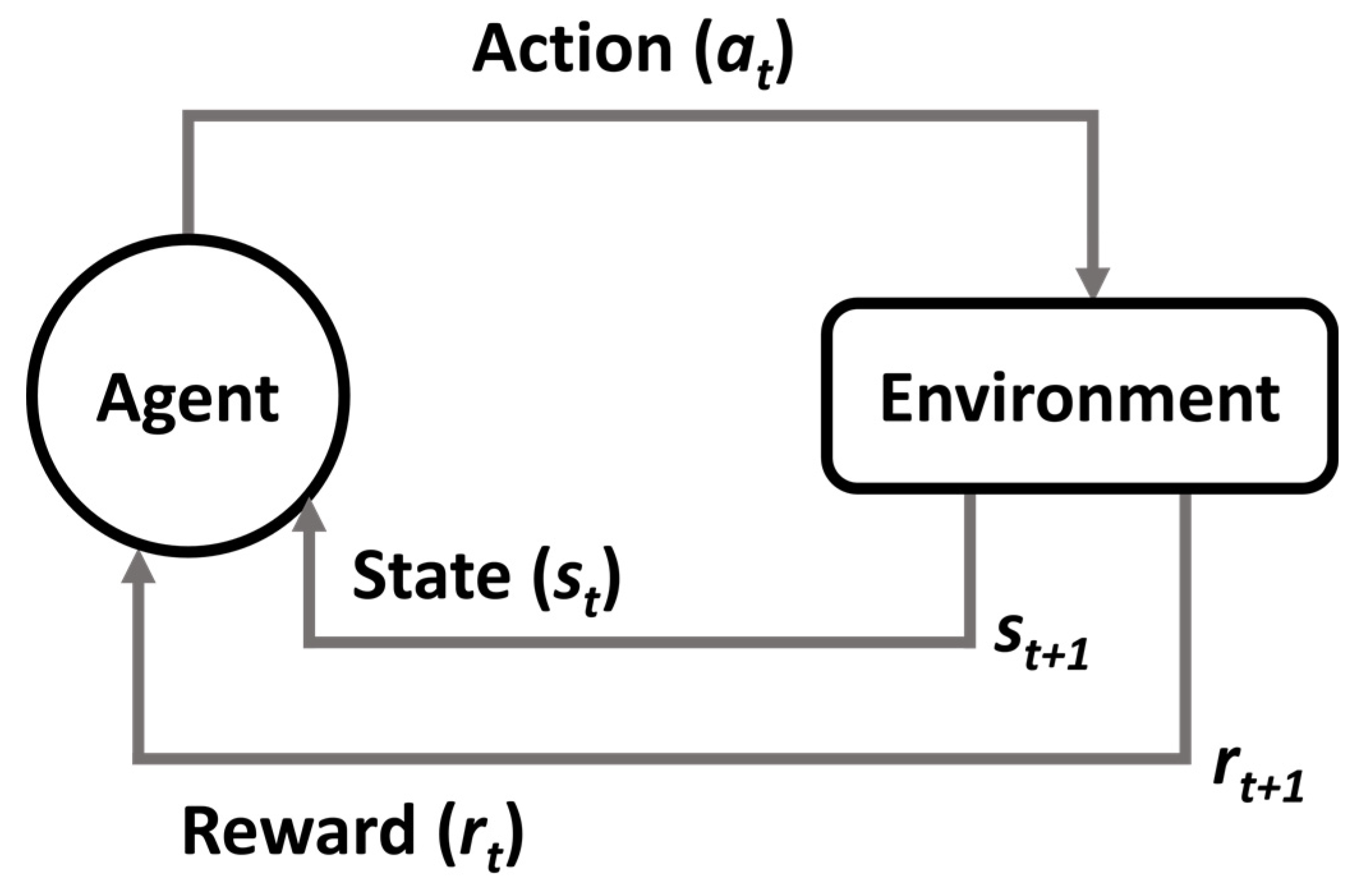
In the typical framing of an RL scenario, an agent performs actions in an environment that are interpreted into a reward and a representation of the state and fed back into the agent. This is illustrated in Figure 1. Here, the agent is the learner and the decision-maker. The environment is the system that it interacts with, comprising everything outside the agent. The action is all the possible moves that the agent can make. The state is the current situation returned by the environment. The reward is an immediate return sent back from the environment to evaluate the last action by the agent.
At every time step t, the agent executes action at, receives state st, and receives scalar reward rt. The environment receives action at, emits state st+1, and emits reward rt+1 at every time step. Each action influences the agent’s future state. Success is measured by a scalar reward signal. RL selects actions to maximise future reward. The strategy, policy(π), is employed by the agent to determine the next action based on the current state. A policy written π(s, a), describes a way of acting. It is a function that takes in a state and an action and returns the probability of taking that action in that state.
where P is the probability of doing action a in state s.
The value function Vπ(s) is defined as the expected return starting with state s, i.e., s0 = s, and successively following policy π. Hence, the value function estimates how good it is to be in a given state.
where E is expected (future) cumulative reward, R is the sum of future discounted rewards, rt is immediate reward, and γ is discount factor (which is less than 1, as a particular state becomes older, its effect on the later states becomes progressively less; thus, its effect is discounted).
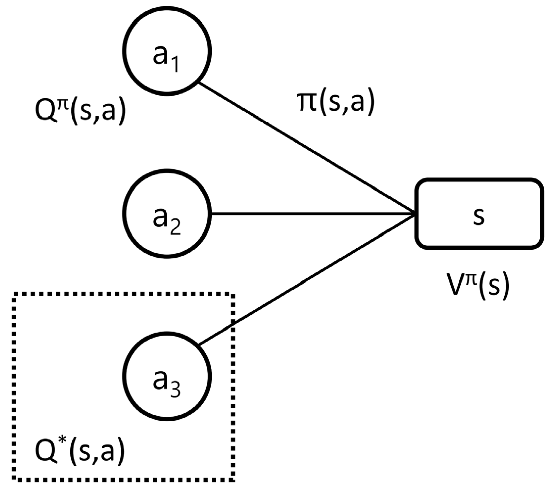
The Q-value function at state s and action a is the expected cumulative reward from taking action a in state s. The Q-value function estimates the adequacy of a state–action pair.
The optimal Q-value function Q*(s, a) is the maximum expected cumulative reward achievable from a given state–action pair. The concept of optimal Q-value function is shown in Figure 2.
To obtain the optimal Q-value, RL breaks the decision problem into smaller sub-problems. Bellman’s principle of optimality describes how to do this [23].
The principle of optimality: An optimal policy has the property that whatever the initial state and initial decision are, the remaining decisions must constitute an optimal policy with regard to the state resulting from the first decision.
The Bellman equation is classified as a functional equation, because solving it means finding the unknown function V, which is the value function. Recall that the value function describes the best possible value of the objective, as a function of the state s. By calculating the value function, the function that describes the optimal action as a function of the state is also found; this is called the policy function. Equations (5)–(8) express this process.
By expressing the above equations as a recursive function and calculating it repeatedly, the optimal value could be obtained.
In power system operation, the agent is the system operator, and the environment is the power system. There are many actions to reduce the short circuit current, but in this study, the separation or merging of bus and line, and movement of the transformer are defined as actions. Agents in the environment that change accordingly can be classified into three categories: short circuit current, overload, and radial system. For these three agents, the state changed after the action is executed can be classified into three categories: decrease in number, increase in number, and no change.
2.1. Action
Before proceeding with the plan to reduce short circuit current using RL, it is necessary to define the action. This study uses bus and line separation actions to reduce short circuit current. The subjects for analysis are 154 kV buses and transmission lines in which excessive short circuit current in the KEPCO grid is greatest. As of 2020, there were 1,213,154 kV buses and 2784 transmission lines (including transformers) in the KEPCO grid. Selecting an action that separates all of these would result in too many possible actions. For bus separation in particular, an additional option involves choices for dividing and connecting the transformer and line after bus separation; this would result in even more actions.
To obtain good results, it is necessary to define the action plan clearly. For the bus separation action, the choice should be limited to actions that effectively reduce the short circuit current while considering the transformer’s capacity and spare capacity. For the line separation action, the choice should be limited to actions that divide the grid into independent grids without making them radial and do not cause overload. Using these conditions, the action set is selected. The bus separation action and line separation action are discussed separately below [36].
2.1.1. Bus Separation Action
Before establishing the action for short circuit current reduction, it is necessary to examine why the short circuit current of the bus is large. As the short circuit current magnitude is inversely proportional to the impedance magnitude, the maximum short circuit current generally occurs at the voltage level for which there are the most transmission lines. In the KEPCO grid, the largest short circuit current occurs at the 154 kV voltage level [36]. Examining the inflow path of short circuit current in 154 kV buses shows that the short circuit current flowing through the transformers is largest at the high voltage level of 345 kV. To reduce this, it is important to separate the 154 kV buses to separate the connected 345/154 kV transformers. For example, if there are a total of four 345/154 kV transformers, the 154 kV buses are separated into the 1st and the 2nd, and two transformers for each are connected to reduce the short circuit current flowing into each 154 kV bus.
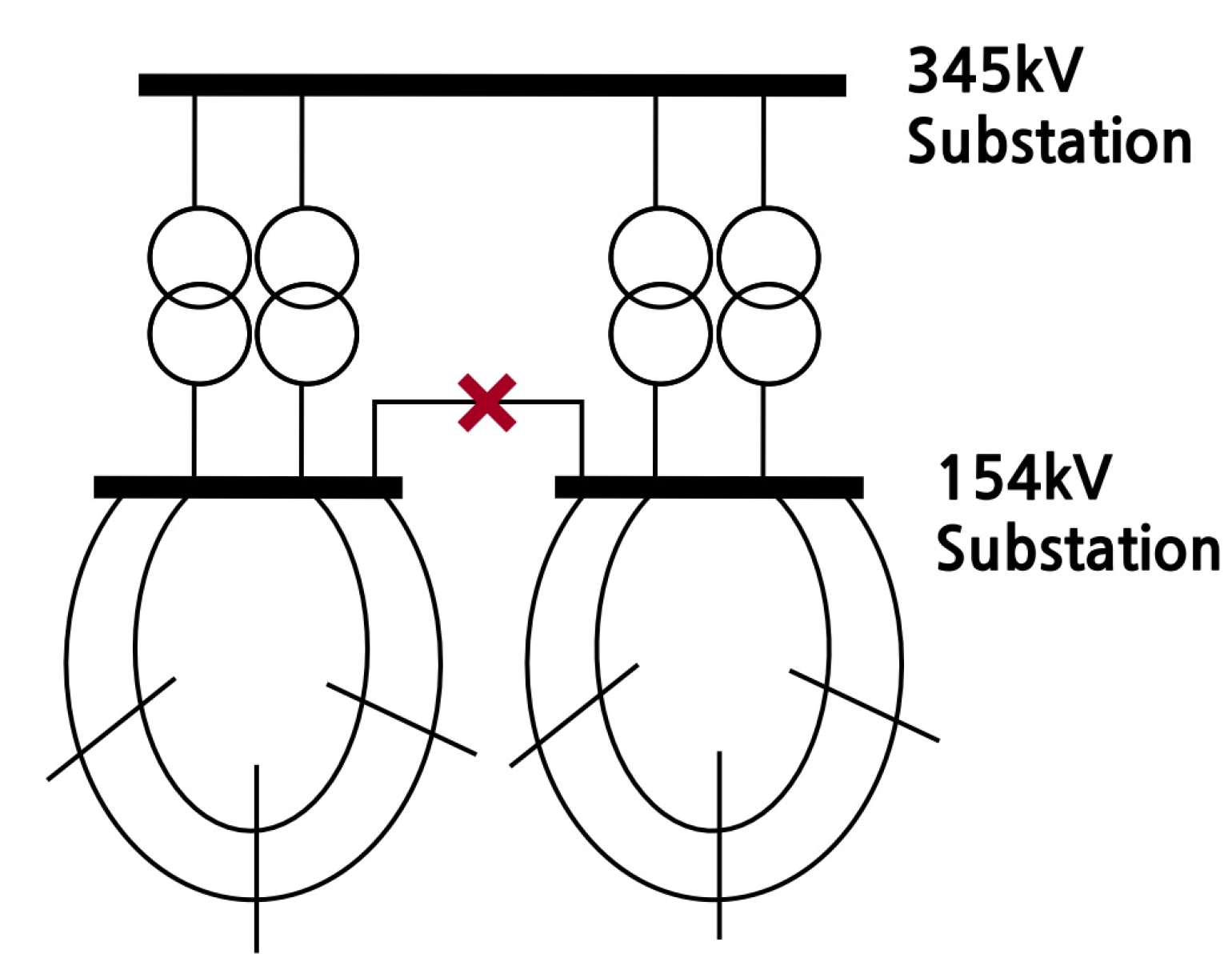
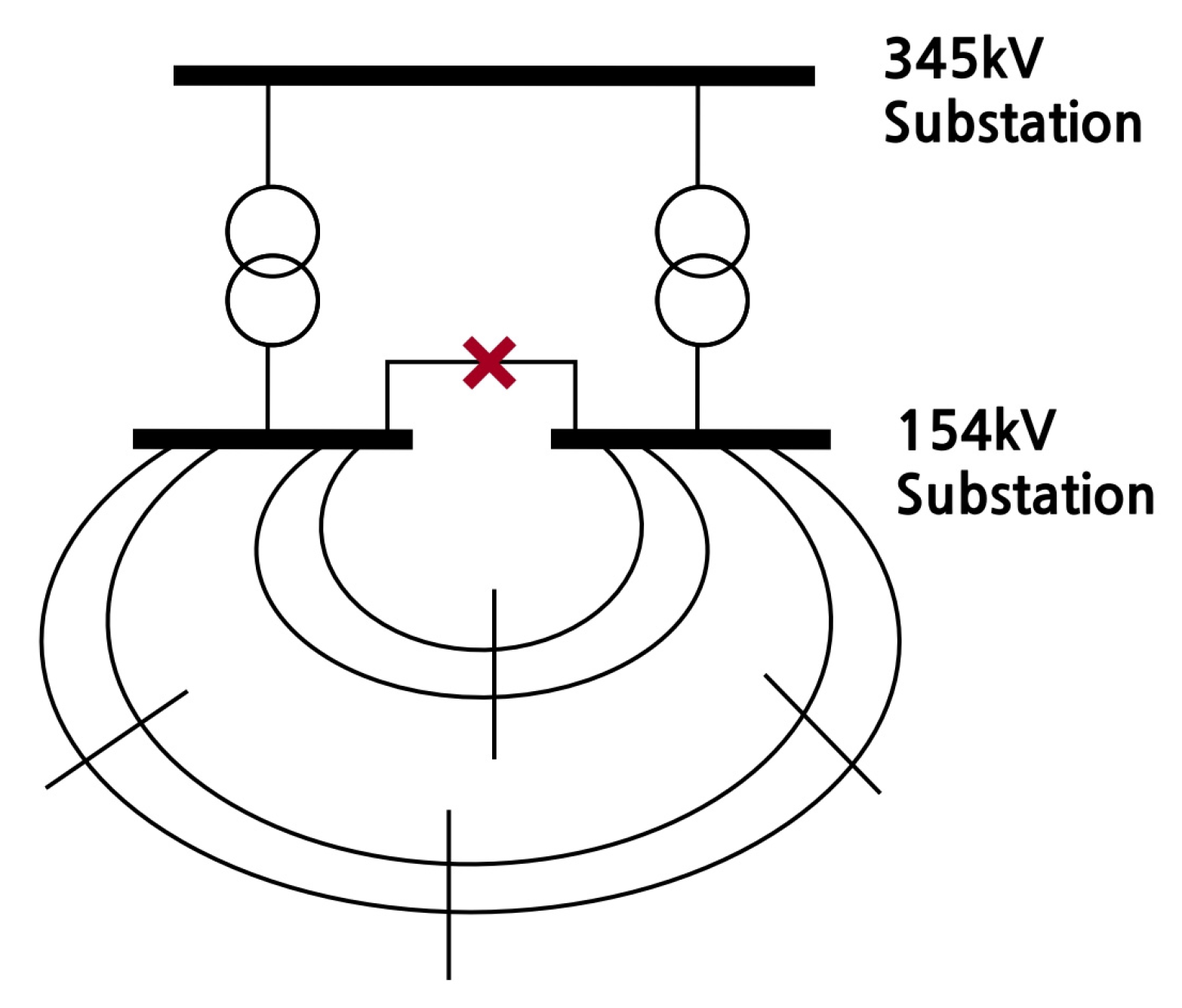
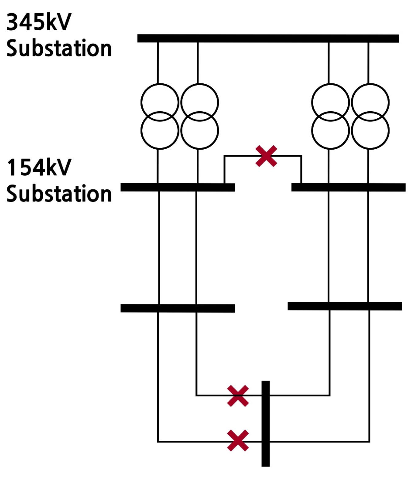
Attention should be paid to whether the transformer is overloaded when disconnecting it in this manner. As the transformers are split for each bus, the total amount of power that each can withstand must be sufficient to cover even a single transformer failure. This is specified in the Korean power grid reliability standards, which states that there must be no problems in operation with an N-1 failure. To satisfy this condition, the transformer must have spare capacity relative to the existing power consumption. If there is spare capacity, then the two transformers can be split while also independently configuring the 154 kV voltage level, resulting in a much greater reduction in short circuit current. However, if there is no spare capacity, transformer failure may result in a violation of the reliability standards. Therefore, the rear end must be connected with a 154 kV level transmission line to eliminate any potential problems. This is illustrated in Figure 3 and Figure 4.
In Figure 1, the transformer has spare capacity. As such, the 154 kV substation can be independently configured to block the additional inflow path of the short circuit current, thereby substantially reducing the short circuit current. In addition, grid stability can be maintained even if a transformer fails, thus complying with the reliability standards. Therefore, if the transformer has spare capacity, an additional line separation action is implemented in a suitable location to prevent the connection of the lower end, and the action to reduce the short circuit current of the grid is selected.
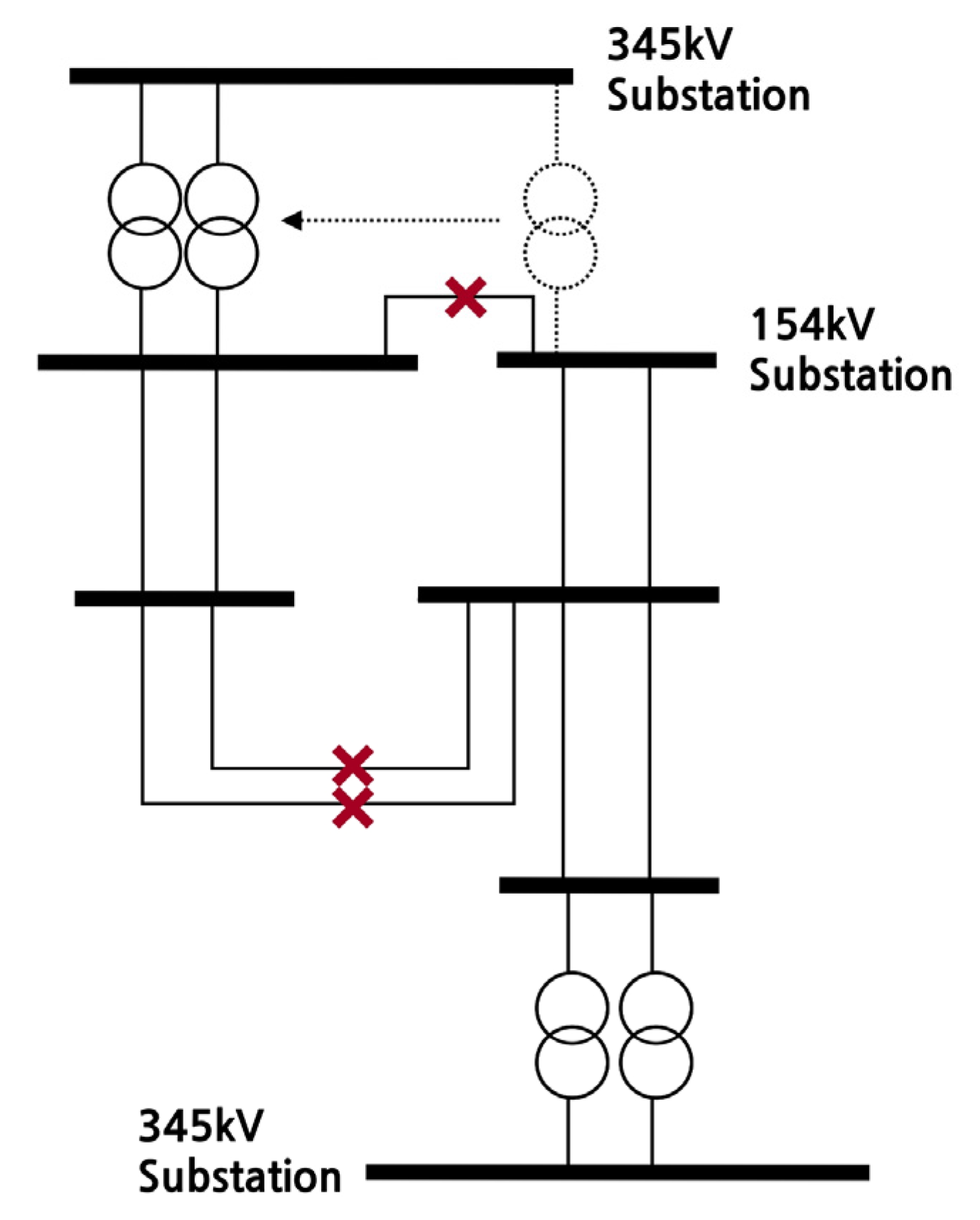
In Figure 2, the transformer does not have spare capacity. Hence, configuring the 154 kV substation independently would violate the reliability standards if a single transformer failed. The lower end should, therefore, be linked to maintain grid stability. When implementing bus separation as above, and as additional line separation is not conducted, separating the transformer can considerably reduce the short circuit current, even though the reduction amount is limited. Accordingly, this is utilised for the bus separation action.
2.1.2. Line Separation Action
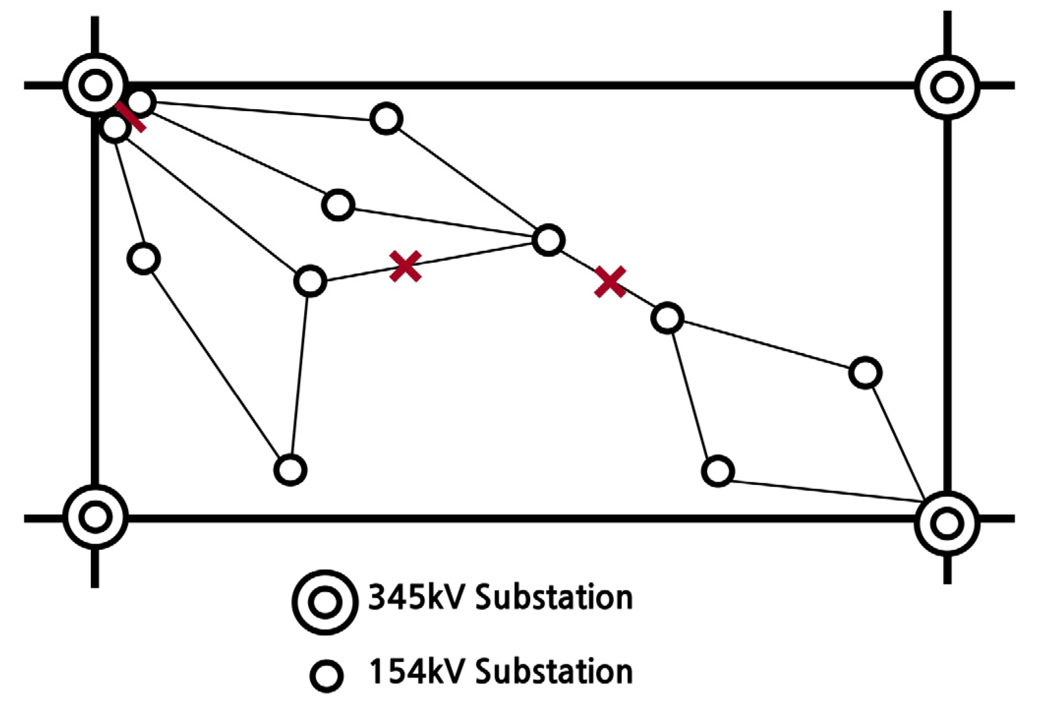
Although line separation is an effective means for reducing the short circuit current of the corresponding bus, separating the line may also result in degraded stability. Moreover, transformer overload and line overload may also occur, which would violate reliability standards. Line separation should, therefore, be minimised. An action used in conjunction with the transformer separation action is effective in this case [36]. If there are no problems with the transformer capacity, then an action is selected that separates the line of the bus where the short circuit current is the greatest at the lower end and independently configures the grid; this maximises the reduction in short circuit current. The action is then selected based on this action. This concept is shown in Figure 5.
2.1.3. Transformer Movement Action
Figure 6 shows the transformer movement action used when the capacity of the transformer is insufficient. If the transformer capacity is insufficient, then the transformer is driven to one side while performing bus separation, the lines are separated at the lower end, and the grid is configured independently and does not violate the power grid reliability standards.
2.1.4. Bus/Line Merging Action
Bus or line merging action is simpler than separation action. It is only necessary to reconnect the separated bus or the open line. If this action is performed, the overload is generally reduced, but conversely, the short circuit current increases.
Figure 7 shows the overall concept of separation, including the separation action for the transformers and lines. By performing separation as below, grid stability in compliance with reliability standards can be obtained along with a substantial reduction in short circuit current. The buses and lines that can be separated from the grid are thus selected based on this action, through which the action is selected.
2.2. Agents and State
In terms of reducing short circuit current, the agents can be classified into three categories: Short circuit current violation (SCCV), overflow violation (OFV), and radial grid violation (RGV). Each item is considered a violation and the number is considered. The closer to zero each item is, the more optimal is the environment. Therefore, the state after taking any action can be classified into three categories according to whether the number of violations increases, decreases, or remains the same.
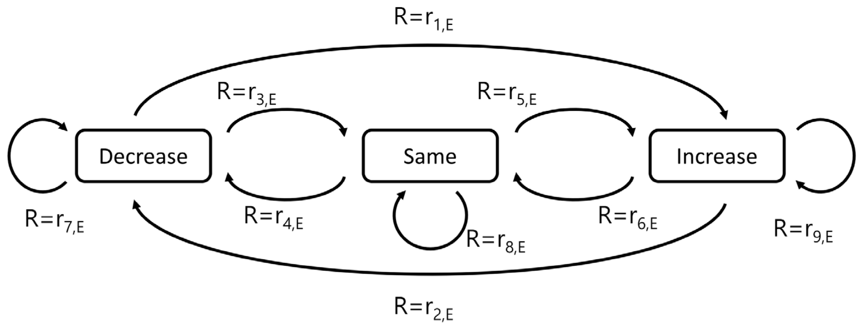
Figure 8 shows the degree of reward according to state change for each agent. In each agent, it is best to go in the direction of decreasing number of violations. Therefore, when an action is performed in the direction that decreases each number, the reward is provided as a positive value. If the number does not change after taking the action, the reward is given as zero. In addition, if one action instead increases the number of violations, the reward is provided as a negative number. By varying the degree of reward, the policy is configured so that the RL can take more effective actions.
The degree of reward for each agent can be the same, but it can also be varied so that more reinforced results can be obtained for the desired environment. As shown in Figure 9, it is possible to lead the direction of the result to the other side by changing the reward according to each agent without setting the degree of reward to a fixed value, or to reinforce the result in the direction the agent wants.
As described above, if the degree of reward is classified into nine types, and the value is different for each agent, the compensation degree for each action, state, and environment can be varied and reinforced in a desired direction to obtain a result.
2.3. Deep Q-Network Algorithm
Before explaining the deep Q-network, Q-learning will be described. Each agent repeats the following steps to maximise the Q-value.
- Choose an action a to perform in the current state, s.
- Perform action and receive reward R(s, a).
- Observe the new state, S(s, a).
- Update: Q’(s, a) ← R(s, a) + γmax{Q’(S(s, a),a)}
Through the above process, an action that maximises the Q-value is selected, which is called greedy action selection. However, if the action that maximises the Q-value is only taken here, the opportunity to learn about various environmental changes would be lost. This would result in optimisation failure, called local optimum. Therefore, to obtain the global optimum, a certain non-greedy action needs to be selected. In other words, choosing an action that gives a rather small reward rather than an action that gives the maximum reward has to be learned. This is called explore, and the method of performing explore with a certain probability (ε) is called the ε-greedy method. Therefore, using the ε-greedy method, non-greedy actions can be explored with a certain probability (ε) to learn about various situations. At this time, it is very important to maintain a balance between greedy action and non-greedy action to obtain optimal results.
The deep Q-network can be thought of as a form that combines artificial intelligence learning by combining a neural network with Q-learning. To formulate this in order to create an algorithm, the Q-value function is first approximated to the Q-network:
If the objective function is developed in the direction of reducing the difference between the current Q-value and the target Q-value in a mean-square error (MSE) method, the equation is as follows:
where U(D) is replay memory, θ is the parameter of the neural network, and θ− is the old parameter.
Using the above equation, the gradient descent method is applied to find the optimum value. Replay memory D appearing here is called experience replay, which stores a dataset of the agent’s experience excluding other relationships. If the reward rt is received after selecting action at in state st and the new state being observed is st+1, the transition (st, at, rt, st+1) is stored in replay memory D. The transitions stored in the memory are used for the optimised MSE, and in some cases, the minibatch is partially executed to improve the speed and the optimisation result. The process for this is expressed in Algorithm 1.
| Algorithm 1 Deep Q-Network algorithm |
| Initialise replay memory D to capacity N Initialise action–value function Q with θ Initialise target action–value function Q with θ− = θ For episode = 1 to num episodes do For t = 1 to T do With probability ε select a random action at, otherwise select at = maxaQ(s, a; θ) Execute action at in emulator and observe reward rt and state st Store transition (st, at, rt, st+1) in D Sample random minibatch of transitions (sj, aj, rj, sj+1) from D Perform a gradient descent step on Lj(θ) with respect to the network parameters θ End For End For |
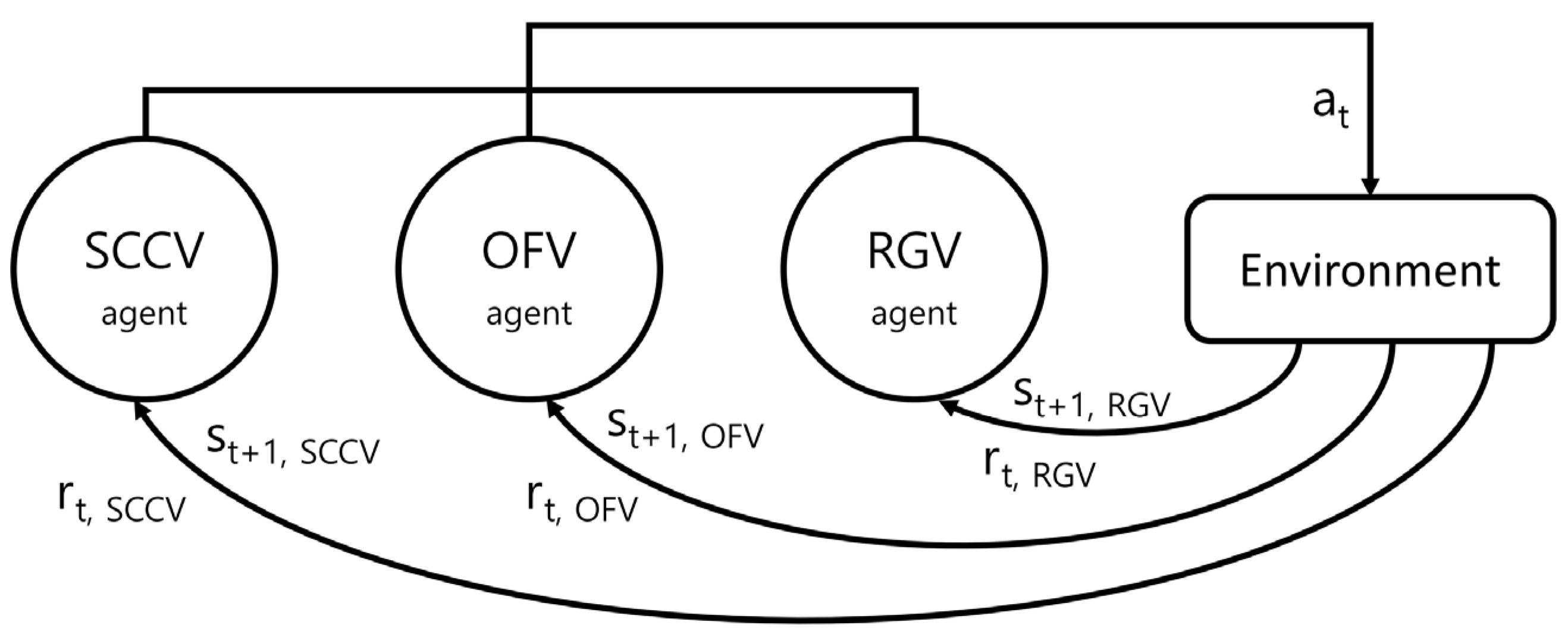
As there are three types of agents in this study, the state and reward according to the action are also divided into three types. Every action causes a change in the environment and a different effect on each agent. Therefore, one action is executed, and each pair of agent state and reward is given accordingly. This concept is shown in Figure 10.
Accordingly, the objective function is also transformed, and the form that adds the optimisation function for each agent becomes the final objective function. This is shown in the following equation:
3. Results
3.1. Applied System and Simulation Conditions
The 8th power grid supply and demand plan was used for grid analysis to minimise the sites exceeding the fault capacity, and the power grid data from 2018 to 2025 were used to verify the effectiveness of the proposed method. In the grid data, minimal bus separation and line separation should be performed in advance for 345 kV buses to ensure that there is no excessive short circuit current for these buses. For the 154 kV buses, both bus separation and line separation were removed, and an integrated grid was created. Additionally, for short circuit current analysis, all generators in the power grid were turned on, and sub-transient impedance was used for generator impedance to generate the maximum short circuit current.
To yield meaningful optimisation results from various simulations that can be applied to actual power grids, the range for each variable must be set. First, the number of buses with short circuit current that exceeds the breaker capacity must be zero to comply with the reliability standards. Second, the number of overloaded lines and transformers must also be zero to comply with the reliability standards. Third, radial systems should not be created after line separation or bus separation. As these three contents are implemented with an agent, it moves in the optimal direction as RL is executed.
The number of separable buses and lines used for each year are shown in Table 2. The number of merged buses and lines, and the number of transformers to be moved can be considered to be included in the separation plan, so values are not set separately.
The results obtained in this study were compared with the results manually generated when making the 8th power grid supply and demand plan before verifying the effect [2].
3.2. Simulation Results
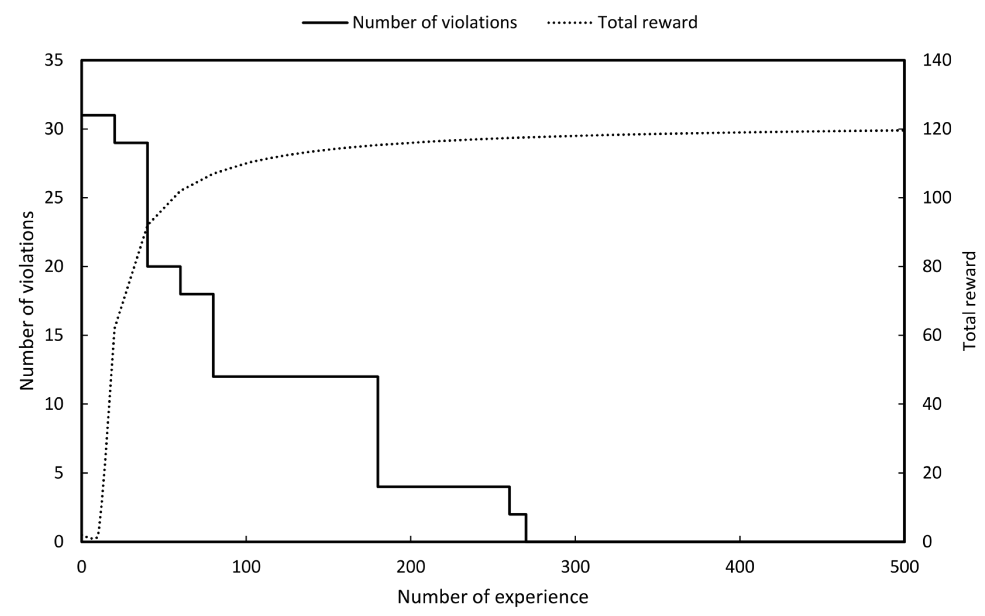
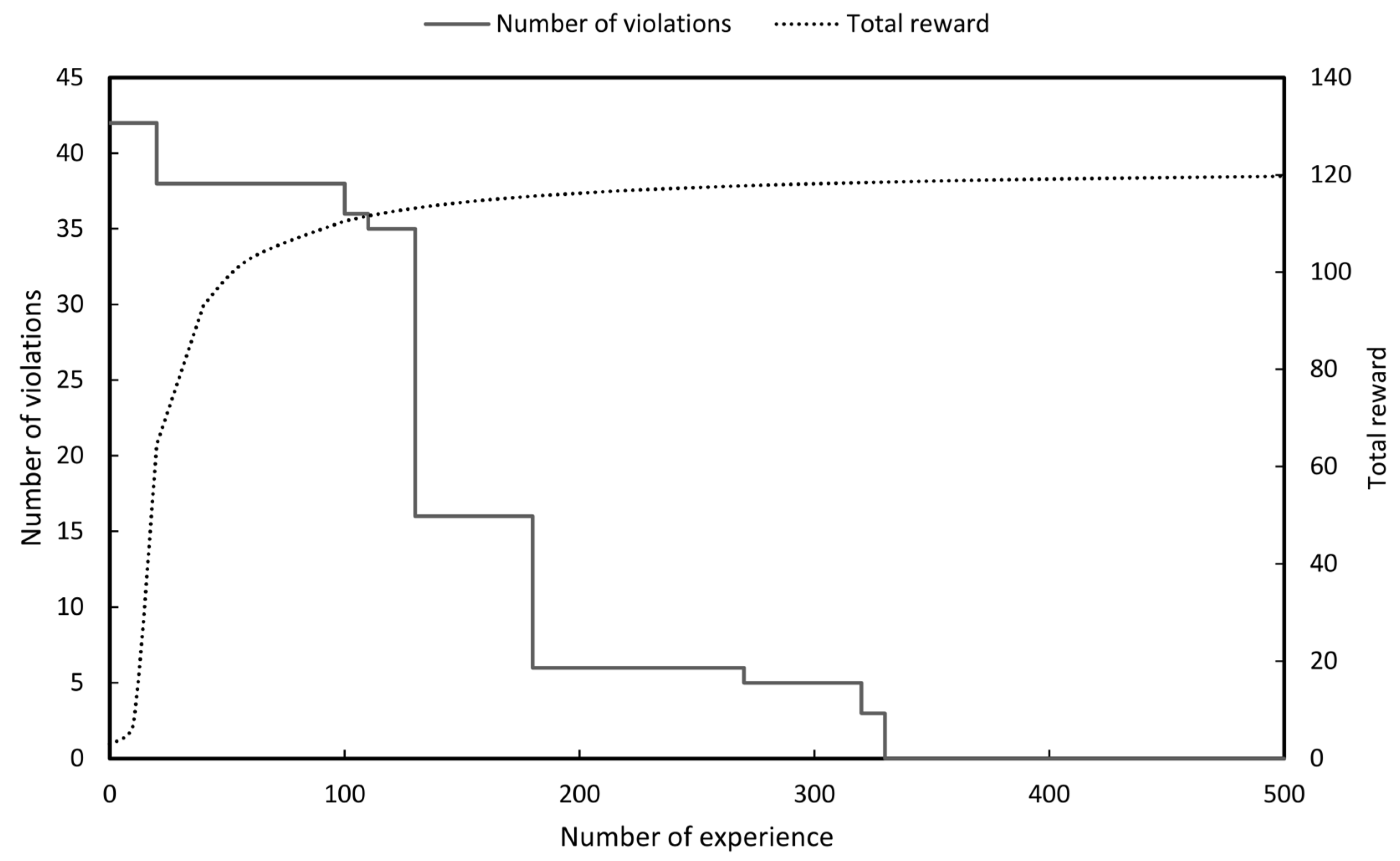
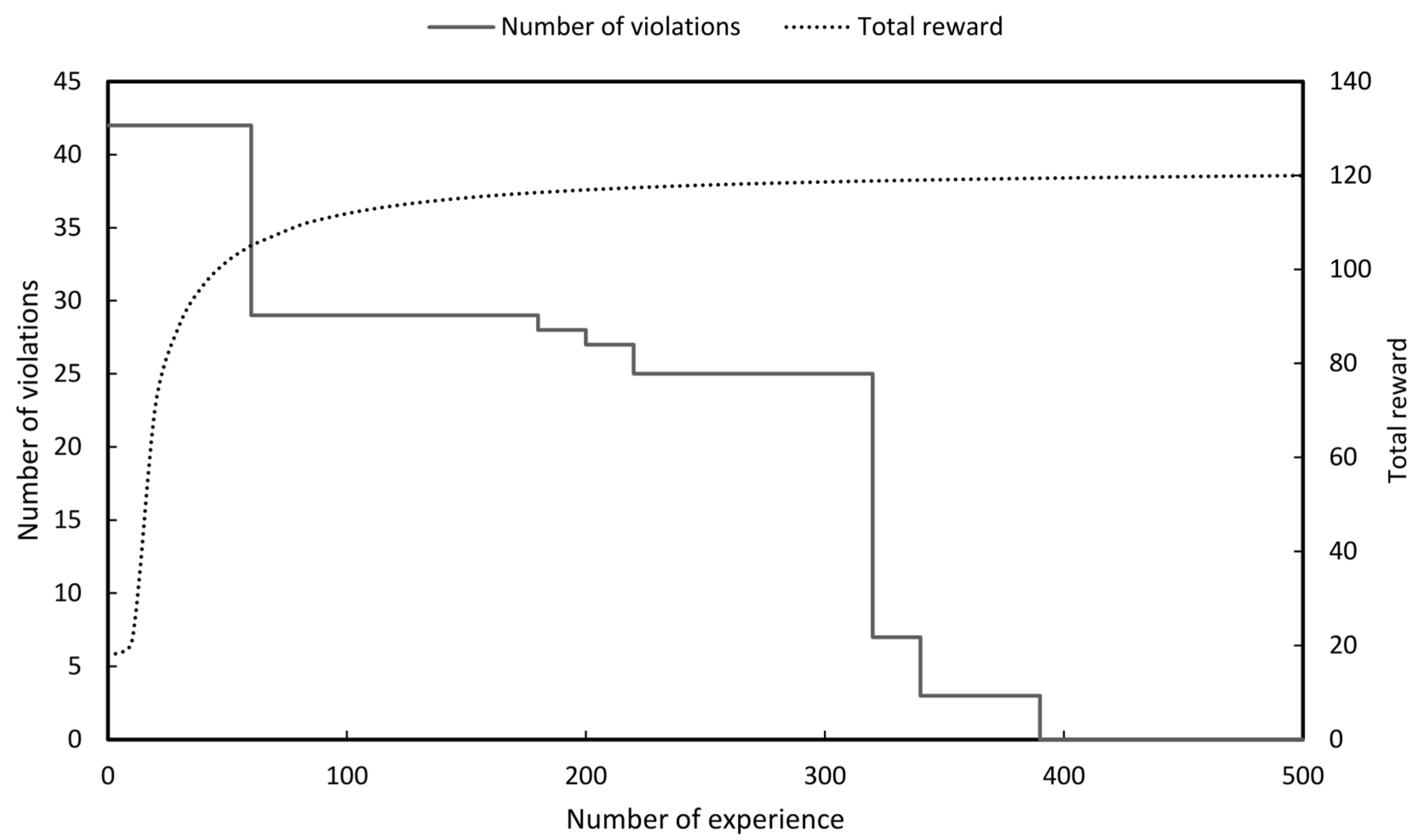
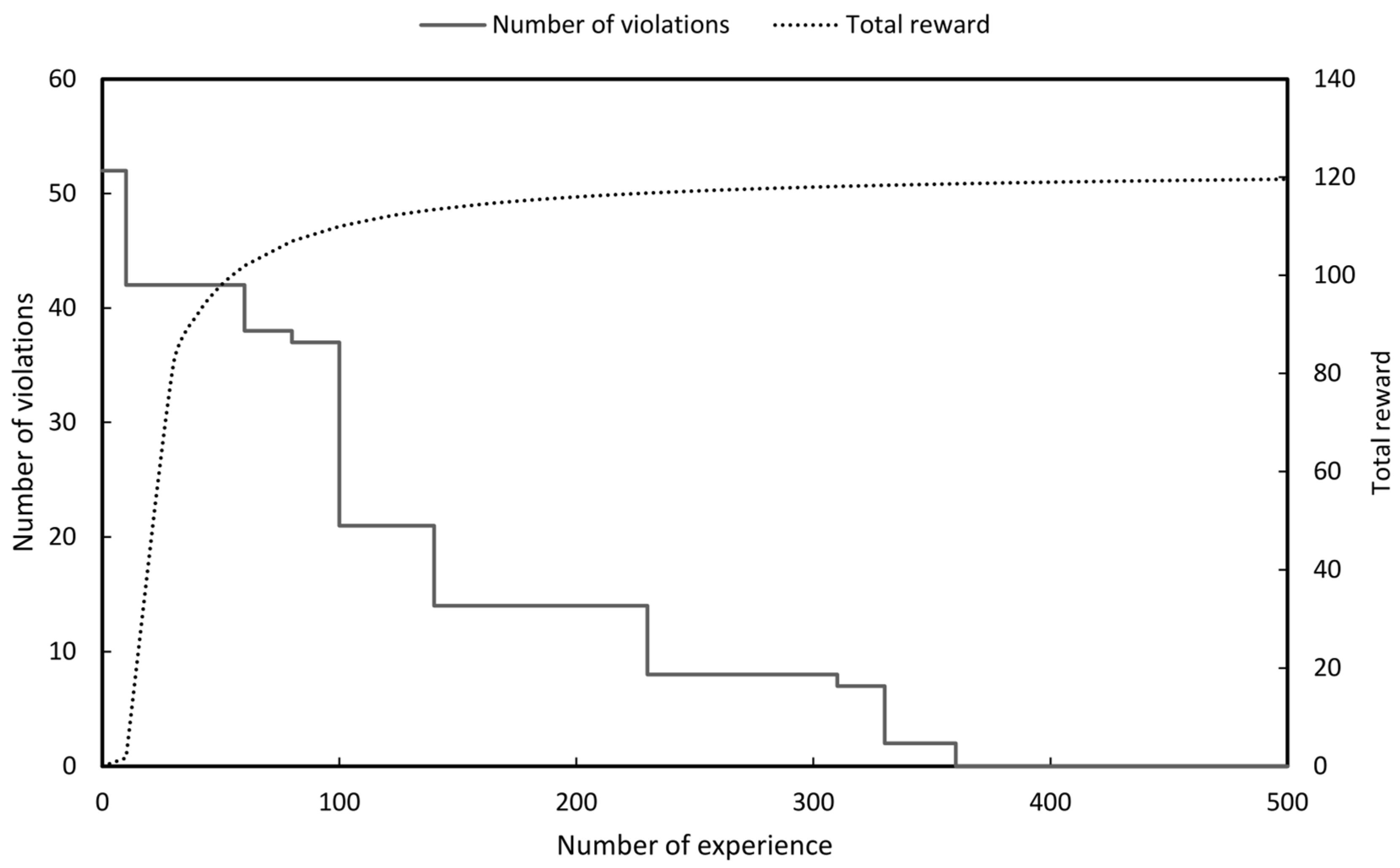
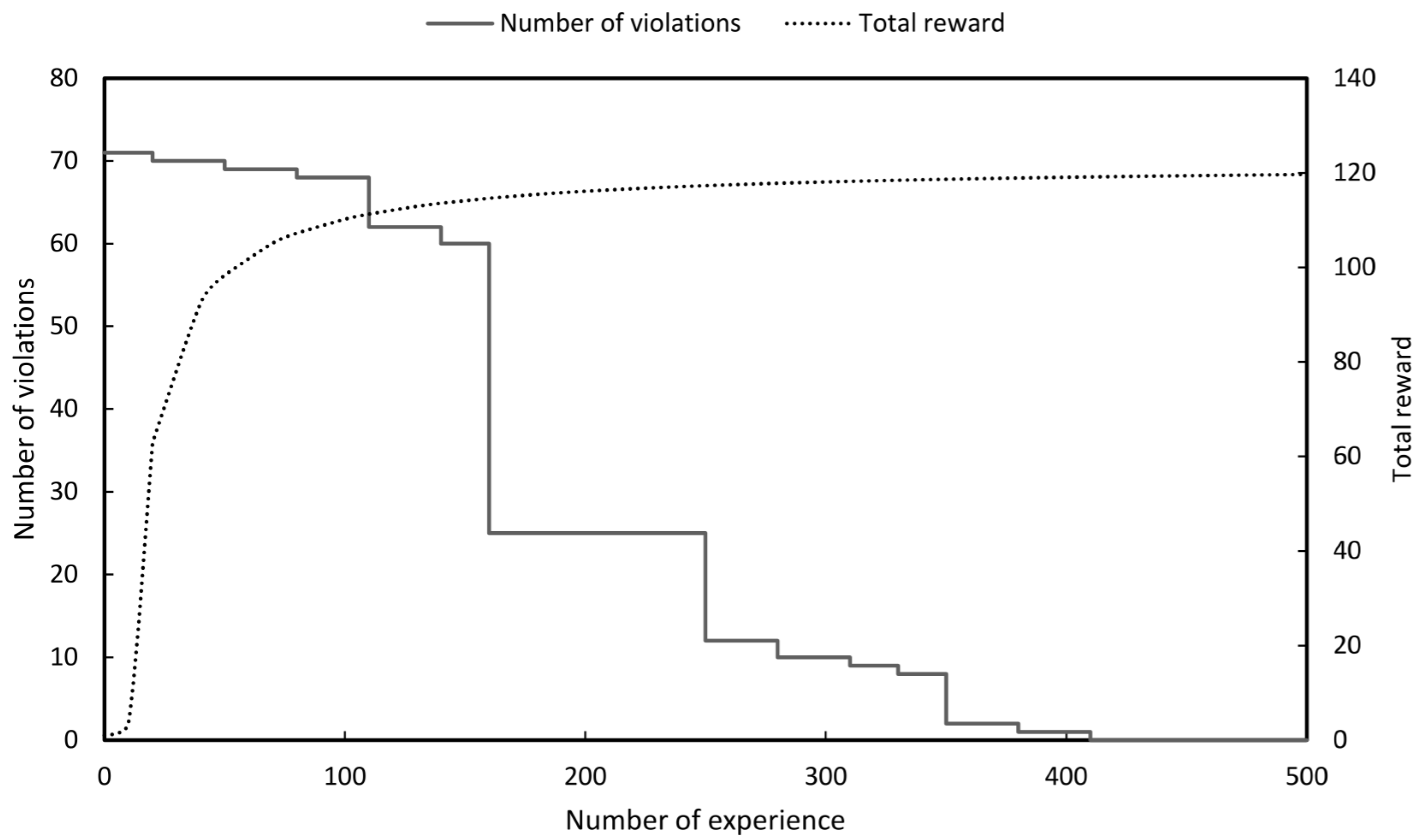
Simulations were performed for the eight years from 2018 to 2025 and the purpose of RL was to maximise reward which is to make the number of violations (SCCV OFV and RGV) of each agent zero.
In practice in a situation where all violations are zero the number of bus separations and the number of line separations should be minimised. Therefore, even if the reward continues to increase the best result in system operation is to adopt the bus separation actions and the line separation actions at the moment when the violation becomes zero rather than selecting the value thereafter.
As shown in Figure 11, Figure 12, Figure 13, Figure 14, Figure 15, Figure 16, Figure 17 and Figure 18 the numbers of violations could be reduced to zero in all graphs with the RL. Table 3 shows the final number of bus separation actions and line separation actions obtained for each year. To compare the results of the RL with the optimal results the number of bus and line separations applied to the 8th basic plan were imported and compared [2]. In the 8th basic plan when separating the bus and lines they were all manually heuristically executed.
As a result of performing the RL even though the number of violations was made all zeros the number of separate buses and lines could be reduced compared to the existing results. This can be said to be the result of obtaining the highest stability without violating the reliability.
There are numerous methods for reducing short circuit current and reducing the number of buses exceeding the breaker capacity. To solve this problem many simulations must be performed manually. However, as shown in this study, defining equations in RL form that can be applied to actual grids’ optimal results can be obtained via the deep Q-network. RL can be used to create effective short circuit current reduction methods systematically for the 9th power grid supply and demand plan in the future and this plan can also be continuously utilised.
4. Conclusions
This paper proposed an RL-based optimisation technique that finds the optimal bus and line separation actions for reducing short circuit current in a power grid. This is accomplished by defining the bus and line separation actions systematically which are the traditional techniques for reducing short circuit current. In this manner optimisation is performed to find the optimal short circuit current reduction method from among numerous possibilities. In particular this paper presented a technique for selecting the bus and line separation actions that can be applied to actual power grids. Using this technique to reduce the number of actions and required replay memory decreases the time required to obtain the RL optimisation result.
RL is effective in determining a method when there is no ideal solution. In particular it is highly suitable for reducing short circuit current using bus and line separation measures. Future studies can enhance the performance of RL by further improving its reward function and further refining and limiting the actions with policy. This technique will contribute greatly to the creation of a power grid supply and demand plan database that will be frequently used in the future.
Funding
This research was funded by Korea Institute of Energy Technology Evaluation and Planning grant number 20193510100040 and Korea Electric Power Corporation grant number R18XA06-65.
Conflicts of Interest
The author declares no conflict of interest.
References
- 8th Basic Plan for Electricity Supply and Demand. Available online: http://www.motie.go.kr/motie/ne/presse/press2/bbs/bbsView.do?bbs_seq_n=160040&bbs_cd_n=81 (accessed on 29 December 2017).
- Han, S.; Ha, Y. A study on the setting of fault current limit for KEPCO’s future system. In Proceedings of the International Council on Electrical Engineering Conference, Hong Kong, China, 3 July 2019. ICEE19J-44. [Google Scholar]
- Wang, L.; Chiang, H.-D. Toward Online Bus-Bar Splitting for Increasing Load Margins to Static Stability Limit. IEEE Trans. Power Syst. 2017, 32, 3715–3725. [Google Scholar] [CrossRef]
- Shen, Z.; Tang, Y.; Chiang, H.-D. Toward Online Line Switching Methodology for Relieving Power System Overloads. In Proceedings of the 2019 IEEE Power & Energy Society General Meeting (PESGM), Atlanta, GA, USA, 4–8 August 2019; IEEE: Piscataway, NJ, USA, 2019; pp. 1–5. [Google Scholar]
- Wang, L.; Chiang, H.-D. Group-Based Line Switching for Enhancing Contingency-Constrained Static Voltage Stability. IEEE Trans. Power Syst. 2019, 35, 1489–1498. [Google Scholar] [CrossRef]
- Koeppi, G.; Blahous, L.; Hager, H. Short-Circuit Current Partitioning in HV Substations in Ring-Bus Arrangement with Redundancy. IEEE Trans. Power Appar. Syst. 1984, PAS-103, 2651–2658. [Google Scholar] [CrossRef]
- Koeppl, G.; Stepinski, B.; Frey, H.; Kolbe, W. The Crossed-Ring Arrangement A New Concept for H.V. Switchgear Installations. IEEE Trans. Power Appar. Syst. 1983, PAS-102, 355–363. [Google Scholar] [CrossRef]
- Barkan, P.; Beehler, J.; Reckleff, J. Breaker Contact Behavior with Rapid Sequential Switching Above Fault Rating. IEEE Trans. Power Appar. Syst. 1983, PAS-102, 2476–2485. [Google Scholar] [CrossRef]
- Hamidi, M.E.; Chabanloo, R.M. Optimal Allocation of Distributed Generation with Optimal Sizing of Fault Current Limiter to Reduce the Impact on Distribution Networks Using NSGA-II. IEEE Syst. J. 2018, 13, 1714–1724. [Google Scholar] [CrossRef]
- Yang, H.-T.; Tang, W.-J.; Lubicki, P.R. Placement of Fault Current Limiters in a Power System through a Two-Stage Optimization Approach. IEEE Trans. Power Syst. 2017, 33, 131–140. [Google Scholar] [CrossRef]
- Lee, B.; Sim, J.; Park, K.; Oh, I. Practical Application Issues of Superconducting Fault Current Limiters for Electric Power Systems. IEEE Trans. Appl. Supercond. 2008, 18, 620–623. [Google Scholar] [CrossRef]
- Kim, Y.; Jo, H.-C.; Joo, S.-K. Analysis of Impacts of Superconducting Fault Current Limiter (SFCL) Placement on Distributed Generation (DG) Expansion. IEEE Trans. Appl. Supercond. 2016, 26, 1–5. [Google Scholar] [CrossRef]
- Jo, H.-C.; Joo, S.-K. Superconducting Fault Current Limiter Placement for Power System Protection Using the Minimax Regret Criterion. IEEE Trans. Appl. Supercond. 2015, 25, 1–5. [Google Scholar] [CrossRef]
- El Moursi, M.S.; Hegazy, R. Novel Technique for Reducing the High Fault Currents and Enhancing the Security of ADWEA Power System. IEEE Trans. Power Syst. 2012, 28, 140–148. [Google Scholar] [CrossRef]
- Tosato, F.; Quaia, S. Reducing voltage sags through fault current limitation. IEEE Trans. Power Deliv. 2001, 16, 12–17. [Google Scholar] [CrossRef]
- Esmaeili, A.; Esmaeili, S.; Hojabri, H. Short-circuit level control through a multi-objective feeder reconfiguration using fault current limiters in the presence of distributed generations. IET Gener. Transm. Distrib. 2016, 10, 3458–3469. [Google Scholar] [CrossRef]
- Smith, L. A practical approach in substation capacitor bank applications to calculating, limiting, and reducing the effects of transient currents. IEEE Trans. Ind. Appl. 1995, 31, 721–724. [Google Scholar] [CrossRef]
- Ha, Y.G.; Jeon, W.J.; Chang, B.H. A study on the effects of BTB HVDC for fault current reduction applied metropolitan area in KEPCO Grid. In Proceedings of the 8th International Conference on Power Electronics—ECCE Asia, Jeju, Korea, 30 May–3 June 2011; pp. 2962–2969. [Google Scholar]
- Labios, R.; Song, H. Determining the placement of BTB converters for fault current reduction in a power system by using a hybrid GA-Tabu search method. In Proceedings of the 2014 Joint 7th International Conference on Soft Computing and Intelligent Systems (SCIS) and 15th International Symposium on Advanced Intelligent Systems (ISIS), Kitakyushu, Japan, 3–6 December 2014; pp. 5–8. [Google Scholar]
- Xi, X.; Gao, X.; Huang, W.; Li, S.; Zhao, Y.; Lv, C. Application Analysis of Resistor Superconducting Fault Current Limiter in MMC-HVDC System. In Proceedings of the 2019 IEEE Sustainable Power and Energy Conference (iSPEC), Beijing, China, 21–23 November 2019; IEEE: Piscataway, NJ, USA, 2019; pp. 2260–2264. [Google Scholar]
- Yoon, M.; Park, J. A study of HVDC installation in Korean capital region power system. In Proceedings of the 2012 IEEE Power and Energy Society General Meeting, San Diego, CA, USA, 22–26 July 2012; IEEE: Piscataway, NJ, USA, 2012; pp. 1–5. [Google Scholar]
- Kaelbling, L.P.; Littman, M.L.; Moore, A.W. Reinforcement Learning: A Survey. J. Artif. Intell. Res. 1996, 4, 237–285. [Google Scholar] [CrossRef] [Green Version]
- Zhang, Z.; Song, Z.; Huang, S.; Chen, Y.; Mei, S.; Sun, K. An Online Search Method for Representative Risky Fault Chains Based on Reinforcement Learning and Knowledge Transfer. IEEE Trans. Power Syst. 2020, 35, 1856–1867. [Google Scholar] [CrossRef]
- Nguyen, K.K.; Duong, T.Q.; Vien, N.A.; Le-Khac, N.-A.; Nguyen, M.-N. Non-Cooperative Energy Efficient Power Allocation Game in D2D Communication: A Multi-Agent Deep Reinforcement Learning Approach. IEEE Access 2019, 7, 100480–100490. [Google Scholar] [CrossRef]
- Jang, B.; Kim, M.; Harerimana, G.; Kim, J.W. Q-Learning Algorithms: A Comprehensive Classification and Applications. IEEE Access 2019, 7, 133653–133667. [Google Scholar] [CrossRef]
- Ferreira, L.R.; Aoki, A.R.; Lambert-Torres, G. A Reinforcement Learning Approach to Solve Service Restoration and Load Management Simultaneously for Distribution Networks. IEEE Access 2019, 7, 145978–145987. [Google Scholar] [CrossRef]
- Gan, X.; Guo, H.; Li, Z. A New Multi-Agent Reinforcement Learning Method Based on Evolving Dynamic Correlation Matrix. IEEE Access 2019, 7, 162127–162138. [Google Scholar] [CrossRef]
- Park, Y.J.; Lee, Y.J.; Kim, S.B. Cooperative Multi-Agent Reinforcement Learning With Approximate Model Learning. IEEE Access 2020, 8, 125389–125400. [Google Scholar] [CrossRef]
- Da Silva, F.L.; Nishida, C.E.H.; Roijers, D.M.; Costa, A.H.R. Coordination of Electric Vehicle Charging Through Multiagent Reinforcement Learning. IEEE Trans. Smart Grid 2020, 11, 2347–2356. [Google Scholar] [CrossRef]
- Wang, W.; Yu, N.; Gao, Y.; Shi, J. Safe Off-Policy Deep Reinforcement Learning Algorithm for Volt-VAR Control in Power Distribution Systems. IEEE Trans. Smart Grid 2019, 11, 3008–3018. [Google Scholar] [CrossRef]
- Xu, H.; Domínguez-García, A.D.; Sauer, P.W. Optimal Tap Setting of Voltage Regulation Transformers Using Batch Reinforcement Learning. IEEE Trans. Power Syst. 2020, 35, 1990–2001. [Google Scholar] [CrossRef] [Green Version]
- Xu, X.; Jia, Y.; Xu, Y.; Xu, Z.; Chai, S.; Lai, C.S. A Multi-Agent Reinforcement Learning-Based Data-Driven Method for Home Energy Management. IEEE Trans. Smart Grid 2020, 11, 3201–3211. [Google Scholar] [CrossRef] [Green Version]
- Yan, Z.; Xu, Y. Data-Driven Load Frequency Control for Stochastic Power Systems: A Deep Reinforcement Learning Method with Continuous Action Search. IEEE Trans. Power Syst. 2018, 34, 1653–1656. [Google Scholar] [CrossRef]
- Yan, Z.; Xu, Y. Real-Time Optimal Power Flow: A Lagrangian based Deep Reinforcement Learning Approach. IEEE Trans. Power Syst. 2020, 35, 3270–3273. [Google Scholar] [CrossRef]
- Han, S. Optimization method of bus separation and line separation using genetic programming for fault current reduction. Sustainability 2020, unpublished work. [Google Scholar]
- Kim, H.T.; Song, G.S.; Han, S. Power Generation Optimization of the Combined Cycle Power-Plant System Comprising Turbo Expander Generator and Trigen in Conjunction with the Reinforcement Learning Technique. Sustainability 2020, 12, 8379. [Google Scholar] [CrossRef]
Figure 1.
The concept of reinforcement learning.

Figure 2.
The concept of optimal Q-value function.

Figure 3.
Bus separation action when the transformer capacity is sufficient.

Figure 4.
Bus separation action when the transformer capacity is insufficient.

Figure 5.
Line separation action when the transformer capacity is sufficient.

Figure 6.
Transformer move action when the transformer capacity is insufficient.

Figure 7.
Bus and line separation action for reducing short circuit current.

Figure 8.
Reward (R) according to state change for each agent.

Figure 9.
Concept of reward change according to state change for each agent (E: SCCV, OFV, or RGV).

Figure 10.
Concept of action, reward, and state for each agent.

Figure 11.
Result of reinforcement learning (RL) for maximising total reward (2018).

Figure 12.
Result of RL for maximising total reward (2019).

Figure 13.
Result of RL for maximising total reward (2020).

Figure 14.
Result of RL for maximising total reward (2021).

Figure 15.
Result of RL for maximising total reward (2022).

Figure 16.
Result of RL for maximising total reward (2023).

Figure 17.
Result of RL for maximising total reward (2024).

Figure 18.
Result of RL for maximising total reward (2025).


Table 1.
Features of each fault current reduction method.
| Method | Systemic Influence | Cost | Installation Time |
|---|---|---|---|
| Bus/Line separation | Stability declined | Very low | No |
| Current-limitting reactor | Stability declined | Low | Few months |
| Replacing circuit breaker | Increase capacity | Medium | Few years |
| Back-to-back system | Additional space | High | Several years |
| High impedance transformer | Increase loss | Medium | Few months |
Table 2.
Number of bus separation actions and line separation actions for each year.
| Year | No. of Bus Separation Actions | No. of Line Separation Actions |
|---|---|---|
| 2018 | 1210 | 2780 |
| 2019 | 1210 | 2782 |
| 2020 | 1213 | 2784 |
| 2021 | 1216 | 2788 |
| 2022 | 1217 | 2792 |
| 2023 | 1220 | 2801 |
| 2024 | 1222 | 2805 |
| 2025 | 1225 | 2813 |
Table 3.
Comparison of the results of RL versus the number of bus and line separations applied to the 8th basic plan.
Table 3.
Comparison of the results of RL versus the number of bus and line separations applied to the 8th basic plan.
| Year | Final Number of Bus Separation Methods | Final Number of Line Separation Methods | ||
|---|---|---|---|---|
| 8th Plan | RL | 8th Plan | RL | |
| 2018 | 60 | 57 | 56 | 54 |
| 2019 | 58 | 52 | 59 | 57 |
| 2020 | 60 | 55 | 56 | 55 |
| 2021 | 64 | 59 | 64 | 63 |
| 2022 | 64 | 58 | 64 | 63 |
| 2023 | 69 | 62 | 63 | 62 |
| 2024 | 68 | 61 | 63 | 61 |
| 2025 | 66 | 61 | 64 | 63 |
Publisher’s Note: MDPI stays neutral with regard to jurisdictional claims in published maps and institutional affiliations. |
© 2020 by the author. Licensee MDPI, Basel, Switzerland. This article is an open access article distributed under the terms and conditions of the Creative Commons Attribution (CC BY) license (http://creativecommons.org/licenses/by/4.0/).
Share and Cite
MDPI and ACS Style
Han, S. Control Method of Buses and Lines Using Reinforcement Learning for Short Circuit Current Reduction. Sustainability 2020, 12, 9333. https://0-doi-org.brum.beds.ac.uk/10.3390/su12229333
AMA Style
Han S. Control Method of Buses and Lines Using Reinforcement Learning for Short Circuit Current Reduction. Sustainability. 2020; 12(22):9333. https://0-doi-org.brum.beds.ac.uk/10.3390/su12229333
Chicago/Turabian StyleHan, Sangwook. 2020. "Control Method of Buses and Lines Using Reinforcement Learning for Short Circuit Current Reduction" Sustainability 12, no. 22: 9333. https://0-doi-org.brum.beds.ac.uk/10.3390/su12229333
Note that from the first issue of 2016, this journal uses article numbers instead of page numbers. See further details here.