The Microsimulation Model for Assessing the Impact of Inbound Traffic Flows for Container Terminals Located near City Centers

Abstract

The growth of container transport places increasing demand on traffic, especially in situations where container terminals are located near the city centers. The main problem is traffic congestion on networks caused by the integration of Heavy-Duty Vehicles and urban traffic flows. The main objective is to identify the critical traffic parameters which cause negative organizational and environmental impacts on the existing and future traffic demand. A micro-level traffic simulation model was implemented for the testing of the proposed framework-based supply, demand, and control layers. The model was generated and calibrated based on the example of a mid-size Container Terminal “Brajdica” and the City of Rijeka, Croatia. The results indicate that the critical parameters are Queue Length on the approach road to the Container Terminal and the Stop Delay on the main city corridor. High values of these parameters cause negative effects on the environment because of increased fuel consumption and the generation of extra pollution. Due to this problem, a sensitivity analysis of the traffic system performance has been conducted, with a decrement of Terminal Gate Time distribution by 10%. After re-running simulations, the results indicate the impact of subsequent variation in Terminal Gate Time on the decrease of critical parameters, fuel consumption, and vehicle pollution.

1. Introduction

Broad usage of containers in shipping and increasing demand for container transport have a strong influence on container terminals (CT) and their development. In most of the CTs, increased demand is perceived as a capacity problem causing berth congestion or lack of storage space [1]. However, increasing storage reception or constructing additional parking lots for external trucks is a costly and often unfeasible solution that requires a lot of space. Congestion may appear on Terminal Gates and on approaching roads outside the CT, causing negative effects on the overall transportation system. Many CTs in the world are placed near the urban areas, which contributes to traffic and environmental pressures [2]. Internal terminal handling equipment and vehicles generate carbon emissions and contribute to air pollution in the port surrounding area [3,4]. Ports have a substantial impact on urban development resulting in a strong cause-effect connection between maritime and land transport [5].

One of the main problems is traffic congestion caused by the shared use of roads in the vicinity of CTs. Traffic flows on main approaching arteries consist mainly of Heavy-Duty Vehicles (HDVs) transporting containers to and from CTs. Therefore, those roads should be designed according to the projected volume and rate of flow with enough capacity according to traffic structure and transport demand. Congestion occurrence on approaching roads near ports may be caused by long procedures of supervisory activities (documentation check procedures), HDVs control at the terminal gate and checkpoints, mismatches between the arrivals and departures of HDVs, or the random distribution of arrivals and delays occurring on main urban arterials or suburban highways as a result of interaction with urban traffic flows. That was the topic of various research papers such as [6,7,8,9]. Long quays at terminal gates located nearby CT cause an increment in vehicle fuel consumption and higher emissions that negatively affect local and global urban environment.

Various microsimulation tools for traffic parameter’s computing may be used to measure the efficiency and capacity limitation of the access roads in absorbing existing and future loads caused by HDVs and increasing container transport demand. They were employed to explore the results of microsimulation model applications based on case studies for various capacities of CTs [10,11].

The aim of this research is to identify the critical traffic parameters affecting traffic flow on approaching roads caused by HDVs, based on existing and projected CT transport demand scenarios of medium-size CTs located near urban areas, to support strategic management decision making.

In this paper, traffic system performance and critical values of the aggregated traffic streams are modeled and analyzed, using the microscopic simulation method. The next section describes the methodology used in the research with a specific focus on microsimulation programming and traffic scenario management. The following section describes the model set-up with key traffic parameters, the research area, and the road network design based on the CT “Brajdica” (Rijeka, Croatia) case study. The last section presents simulation results and analyses the findings to be subject to further discussion and research.

2. Literature Review

The previous research in the field may be classified into four main categories according to the objects and methods applied:

• Reducing truck congestion at ports and capacity problems at ports
• Reducing queues at CT gates and reducing greenhouse gas emissions
• Simulation methods to support flow management in adjacent port-urban networks
• Macroscopic approach to urban traffic management

Lange et al. [12] provided an overview of the existing classification scheme and offered solutions for reducing track congestion at logistic nodes in the port, especially at CTs. They noted the problem of high fluctuation in truck traffic load, which results in long waiting times at gates, but also affects public streets and the performance of other port subsystems. Different approaches to solving these problems include night or off-peak shifts, truck arrival management systems, truck appointment systems, IT monitoring and information systems, etc.

Efficient gate operations are not only important for the efficiency of port operations, but also have a strong impact on the traffic of nearby roads. Maguire et al. [13] conducted a critical review of the published literature on the different gate strategies. The main problem stated is the forced pick-up and deliveries during hours with high traffic demand. The operational strategies include gate appointment systems, extended gate hours of operation, truck buffer areas, and marshaling yards to gather and service trucks according to a pre-determined pattern. Ma et al. [9] pointed out that irregular external truck arrivals at a marine CT lead to long queues and substantial greenhouse gas emissions. They proposed a truck arrival pattern called “vessel dependent time windows” and established an optimization model for the appointment of quotas for each vessel arriving at CT. According to [8], the truck arrival pattern is the key to modeling port area traffic demand. Poor knowledge of a port area traffic flow results in bad network planning and traffic management. The authors raised the problem of road design planning when the port traffic demand is neglected. They proposed an arrival pattern of external trucks for the prediction of traffic demand.

Truck appointment systems are a common approach for the reduction of congestion at terminal gates and many papers have shown that they reduce terminal turnaround time [14,15,16,17]. The truck appointment system was developed in response to heavy congestion on Pacific coast seaports. The common goal is to optimize truck scheduling and minimize gate waiting time and yard processing time.

There is a group of papers related to simulation methods and their implementation in the justification of traffic strategies and policies. Preston et al. [18] explained the benefits of using discrete-event simulation, particularly in identifying where future bottlenecks are likely to form within the port area. They showed how it is possible to reduce future traffic congestion that is expected to be achieved if freight traffic grows by rearranging the port area releasing additional space for vehicles waiting to pass check-in control. Not only future strategies, but short-term measures can be supported by using microsimulation methods for improving traffic conditions in ports, as showed in [19], where a simulation model for the existing road layout is developed. Some alternative solutions have been proposed in network design and gate control to reduce the existing congestion in the Chennai port. Three different traffic models are developed, and different software packages are compared in [20]. The paper presents the advantages and disadvantages of each tool when modeling port traffic conditions. Strategic planning of port systems based on the integration of urban road network and port traffic organization was the subject of the research in [10]. The authors identified conflicts for port-urban traffic environment; namely, the conflict between entering traffic flow and external road network traffic and the conflict inside the port area caused by traffic inside the terminal. They defined the limits of maximum entering traffic flows to limit the queue length and made experiments to provide a stable road traffic and port operation.

A macroscopic approach has been applied by Alonso et al. [21,22] using the Macroscopic Fundamental Diagram (MFD) for traffic monitoring in urban areas and signal control management. In [22], the authors presented a three-step procedure for the implementation of MFD in traffic analysis. The availability of real traffic data is a crucial element in the application of that methodology, hence studies [23,24] introduced a methodology to obtain MFD using combined data from floating cars, loop detectors, and data from GPS-equipped taxi vehicles.

3. Materials and Methods

Several methodologies have been developed to identify the occurrence of the traffic flow on the approaching roads of CT and the main city arteries to quantify and determine the interdependencies of the traffic flow parameters. Most of the methodologies imply the application of mathematical and simulation modelling methods. The advantages of the simulation modelling method are described in [25]. Microscopic traffic models are most effective for presenting and analyzing the initial or future state of traffic situations because microscopic traffic simulation models are based on the simulation of discrete events or vehicle movements during the observed time intervals with an emphasis on the traffic behavior patterns [25]. In recent times, there is another approach to model traffic in urban areas based on the macroscopic scale of monitoring flow and density. The aggregation is done on the network level using the Macroscopic Fundamental Diagram (MFD) for the description and identification of the critical sections and nodes where congestions occur.

In this paper, we have created a microscopic model of a small part of the urban road network of the integrated traffic network that includes access links to the CT. The reason for choosing the micro-level of traffic analysis is the question of access road capacity and geometry in peak periods and the potential impact of increased CT demand in the future. Since this is an important but small part of the urban traffic network, we left out the macroscopic approach in this case for further research.

We defined the traffic zone consisting of the CT gate, approaching road, and the main urban motorway. The microscopic model reproduces the initial traffic condition—flow, density, speed, and measure traffic performances—delays, queues, and travel times on the links and routes within the predefined zone. Depending on the measurement and recorded data from traffic surveys, the goal was to analyze performances and critical points of the network, especially caused by HDVs, with origins and destinations to CT. Then, we used the future demand scenario for container traffic to assess the traffic performances and to identify critical points of the system. Finally, we performed a sensitivity analysis to test possible policy measures to control and neutralize the negative effects of increased demand on traffic performance.

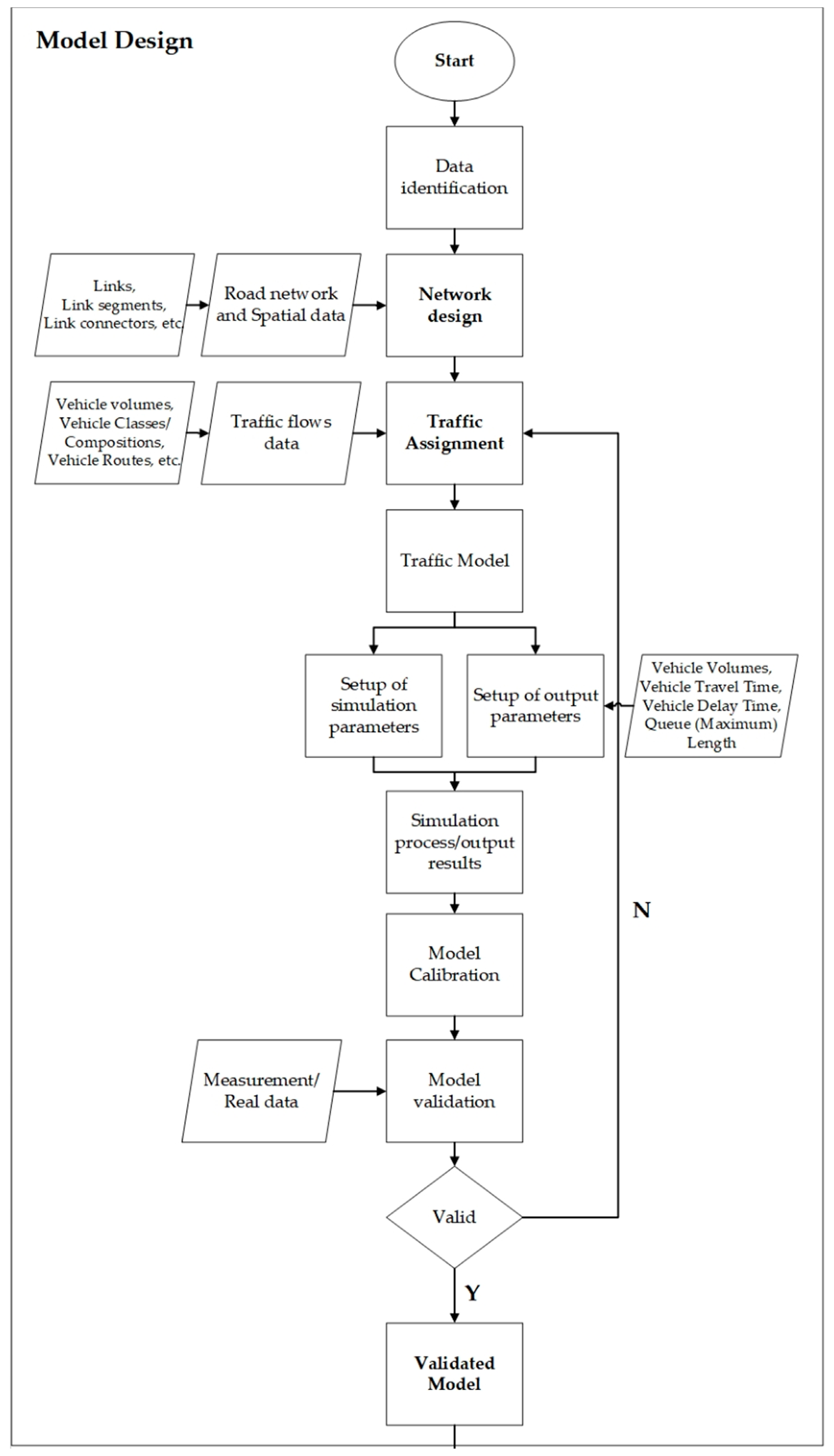
The model design is shown in Figure 1 while the simulation process is shown in Figure 2.

Applying the above methodology, the whole process is divided into the model design and the simulation process (Figure 1 and Figure 2). This includes the following steps:

• Designing the traffic network using supply side data
• Importing the traffic demand data from surveys and record books
• Defining key performance indicators and their incorporation into the traffic model
• Calibration and validation
• Scenario demand management and Traffic Control Management
• Analysis of outputs, evaluation of the control strategy results

In the first step, we identify and collect input data for network design, which we called the supply layer. This layer combines road and spatial data, road segments, and connectors with their attributes (e.g., number of lanes, movement directions, speed limits, etc.). Within this layer we also defined the Terminal Gate as a special object which presents the node where inbound or outbound HDV traffic goes through documentation and security checks when entering CT or leaving the terminal gate. The Terminal Gate object may also have a control feature in the model where different policies may be tested to avoid congestion.

Traffic demand data are collected from surveys and record books in the demand layer and are joined with the network in a process we call a Traffic Assignment. The demand layer combines variable data depending on traffic characteristics and vehicle compositions on the network, including volume during normal and peak hour periods, vehicle classes, vehicle routes, speed distributions, and driving characteristics. Regarding the CT demand data, we used history records from the terminal operator and custom office and corresponding future demand data available from the master plans.

Since we used microscopic simulation for the observation of traffic performances within the limited zone nearby the CT, there is no route choice feature embedded; therefore, the travel time between link sections represents a network cost function. For CT bound traffic, the cost function generally consists of travel time between the road section and the terminal entrance where the Terminal Gate object is located, plus the gate-in time required for HDVs to pass check-in control. The logistic cost incurred within the CT area due to waiting for HDVs to be serviced is not considered here. The time cost function at the Terminal Gate object is always activated when the HDV approaches close enough to the sensor, and their values depend on whether the HDV carries a full or empty container. This is a realistic situation because empty containers do not require the same level of checks as full ones.

To get a representative model applicable for traffic simulation, we defined proper time intervals with typical traffic demand. The typical traffic demand strongly depends on CT activities, i.e., working shifts, schedule of vessel dockings, and shipping arrival/departure patterns. Therefore, we analyzed historical data of the CT activities, the activities that cause traffic peaks. We also identified critical working daytime intervals and peak-hour volumes of HDVs traffic registered at the Terminal Gate control. Based on that, we have generated multiple time intervals of 900 s each within 1 h for two CT working shifts (16 h) as a simulation time frame.

A further step in the model design was the definition of network performance indicators and cross-section road-specific parameters. Key performance attributes are the Number of vehicles per vehicle category, Queue Length, Maximum Queue Length, Delay Time, and Stop Delay Time per vehicle. To obtain desired performance measurement values, specific virtual objects were created: Count, Time, and Queue detectors. These virtual detectors have two important functions. First, they are closely related to traffic performance attributes measurement needed to quantify the impact of HDVs volumes on traffic flow of the integrated city network and consequently the impact of container inland traffic on urban mobility. Second, Count detectors are important because, according to results obtained, model calibration and validation are carried out. We consolidated this under the so-called control layer.

We calibrated the integrated model according to parameters that indicate missing turns in the network and/or virtual queues that are formed outside the network. Further, the validation procedure is carried out to determine whether the representativeness of the model is statistically significant or not. We based the validation process on comparing deviations in the results obtained from the model versus real data results recorded directly on-the-field. If the validation criteria are not satisfied, the demand layer, i.e, traffic assignment inputs, are rechecked and modified accordingly to get more representative data.

For the simulation process, we used a validated model based on initial (basic) and additional (future) HDV demand scenario. Future demand scenarios are based on a port master plan forecast in which the annual growth rate for container traffic of 6% is foreseen. We performed a sensitivity analysis using different traffic control strategies based on Terminal Gate Time (TGT) variations traffic policy and observe the outputs.

4. Model Design

The model is designed following the methodology described in the previous chapter. In the first sequence of model creation, we defined the area of research or target zone. This zone covers the port area of a medium-sized CT located in the urban zone of the city of Rijeka, Croatia. We will present the model design process in detail in this chapter. We will also describe how the sequence output data was defined and collected for the calibration and validation of the model. By the last sequence, we created two scenarios that present Base and Future traffic demand according to the CT throughput.

4.1. Testing Area Description and Network Design

Two main design layers are modeled for the selected area of research where traffic generated from CT is merged with urban area traffic alongside the main city corridor. The area of research is CT “Brajdica” and the city of Rijeka (Croatia). This CT is located within the Port of Rijeka, the biggest Croatian port, which also has the status of E-port. Additionally, it is a part of the Northern Adriatic (NAPA) group of ports. The North Adriatic route is one of the European Gateways for Far-East container traffic with destinations in Central and Eastern Europe. However, the terminal is located within city borders. The main problem is the distribution of cargo to the hinterland, especially for micro-locations, where cargo traffic flows (HDVs) are merging with urban traffic flows.

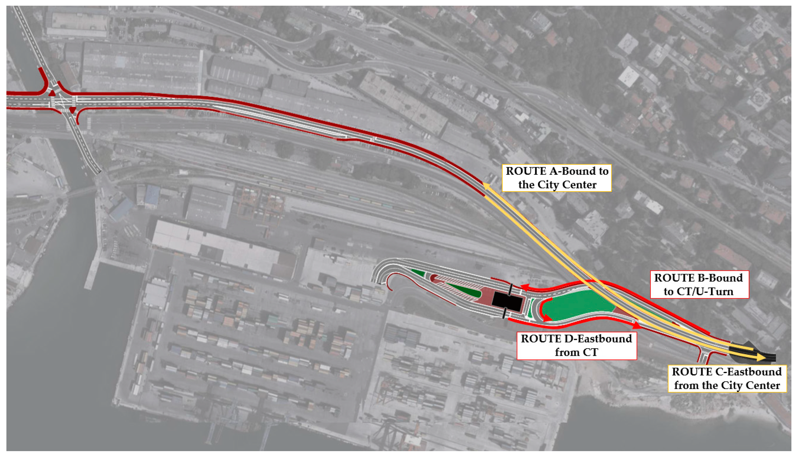
The problem could become even more significant, when the annual growth of container transport and the modal split distribution is taken into consideration. For example, in 2019, the annual growth rate at CT was above 10%. Thus, more problems with traffic congestion on roads nearby may be expected in the future. In this case, a new Terminal Gate has been constructed recently, but it is impossible to eliminate the HDV queues generated when passing through the Terminal Gate control. When the dynamic of arrival becomes more extensive during peak hours, the effects on the overall traffic network around the terminal zone may be more significant, i.e., affect a user’s travel time. It is not insignificant to mention the negative impact on the environment caused by increased pollution from vehicles during a more extended period of travel. The micro-location of the research area with the main traffic routes and detectors for monitoring is shown in Figure 3.

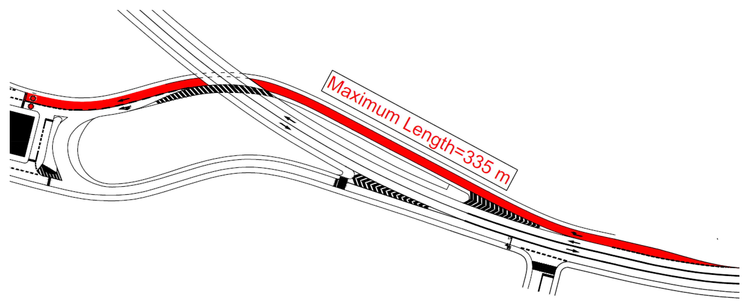
There are four directions or vehicle routes modeled (Figure 3): Route A—bound to the city center, Route B—bound to the CT/U-turn, Route C—eastbound from the city center, and Route D—eastbound from the CT. The focus is put on traffic mixed flows on routes A and B (HDVs and other vehicle categories traffic). On Route B there is also a Terminal Gate control point where HDVs need to wait for security reasons and where check control takes place. The time at the Terminal Gate directly affects the traffic and performance of the traffic flow on the main east-west city corridor. The time at Gate varies depending on the type of containers arriving at the CT (full or empty). Field research has shown that the average time at Terminal Gate for HDVs with a full container is 120 s with a standard deviation of 30 s, and for empties, 30 s with a standard deviation of 10 s. It was observed that the backward queue is formed in a specific situation with a length near to 335 m. That is the maximum length of the approach road heading to CT, which means that congestion may likely occur in the westbound direction toward the city center area (Figure 4).

4.2. Model Data Inputs

For the functionality of the model, a consistent and relevant traffic dataset should be provided. According to the history of container traffic development and terminal operation records, it is observed that traffic demand in specific weekdays is higher than on others. The reason is the shipping and work schedule for the preparation of cargo load. Therefore, we chose three weekdays, particularly Monday, Wednesday, and Friday, as typical weekdays when transport and traffic demand are at a higher level. The workload is concentrated during the daytime, so we have taken one-hour time intervals between 6–22 h for each day. With these dynamics, the CT annual throughput is around 300,000 TEU (Twenty-foot Equivalent Unit).

The traffic volumes data were collected using inductive loop detectors while the validation was performed using data from surveillance video cam recordings.

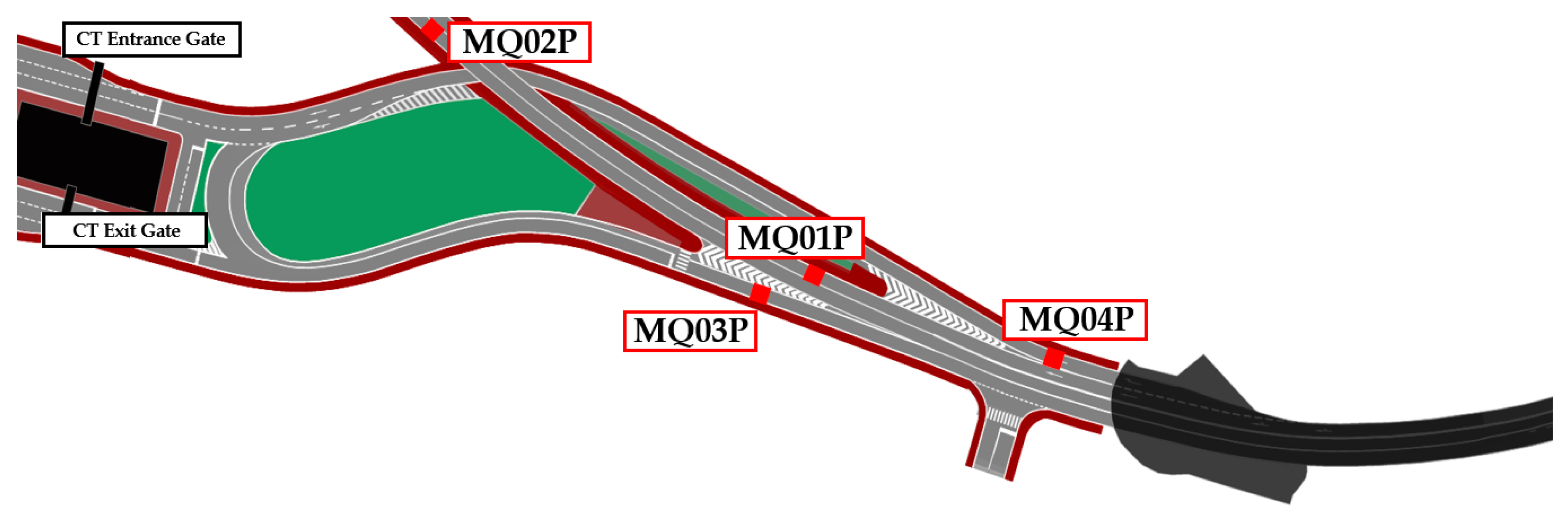
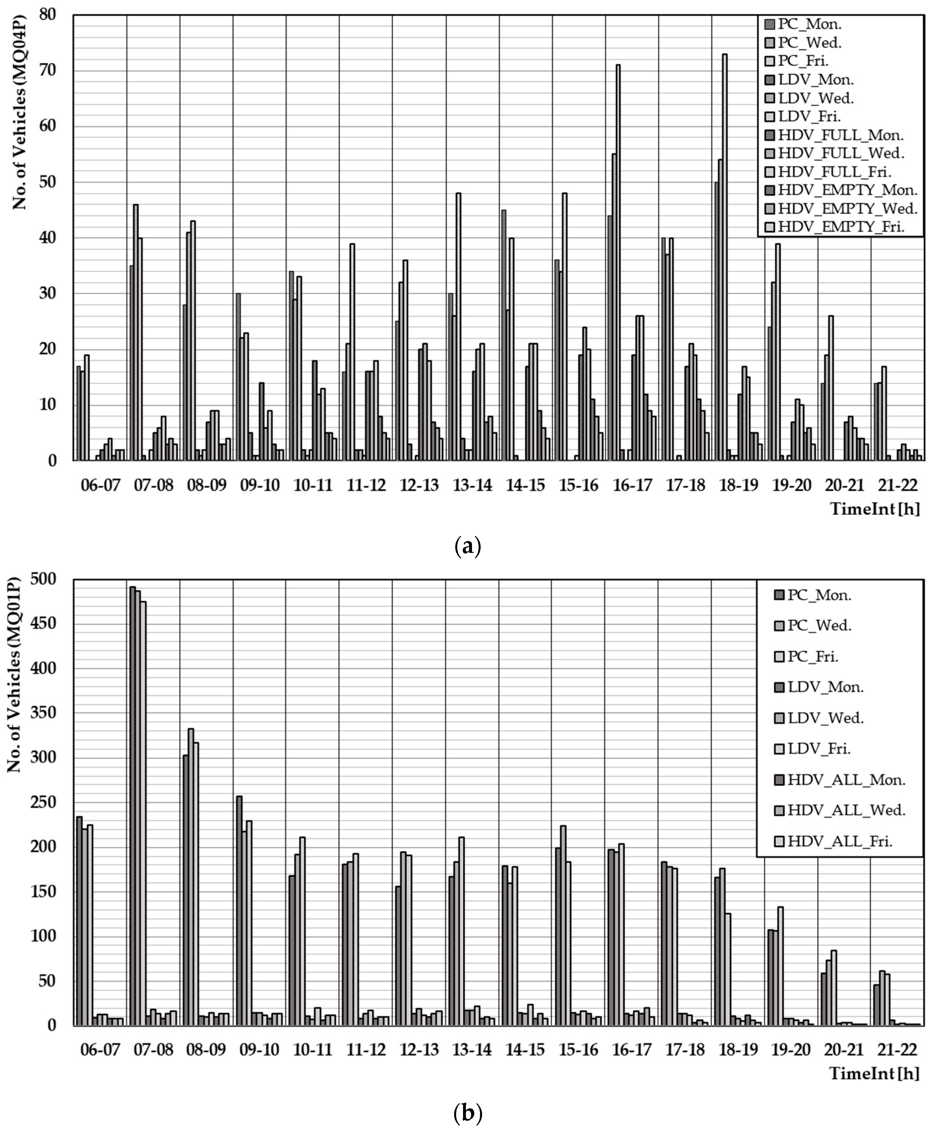
Detectors and video cams are installed on the following locations (Figure 5): Route A (MQ01P), Route B (MQ04P), Route C (MQ02P), and Route D (MQ03P). Volumes are distinguished according to vehicle class type for each route choice; that is, personal cars (PCs), light duty vehicles (LDVs), heavy duty vehicles with a full container load (HDVs Full), and heavy duty vehicles with an empty container load (HDVs Empty). Some vehicle classes are ignored due to their low share and their marginal impacts on traffic flows.

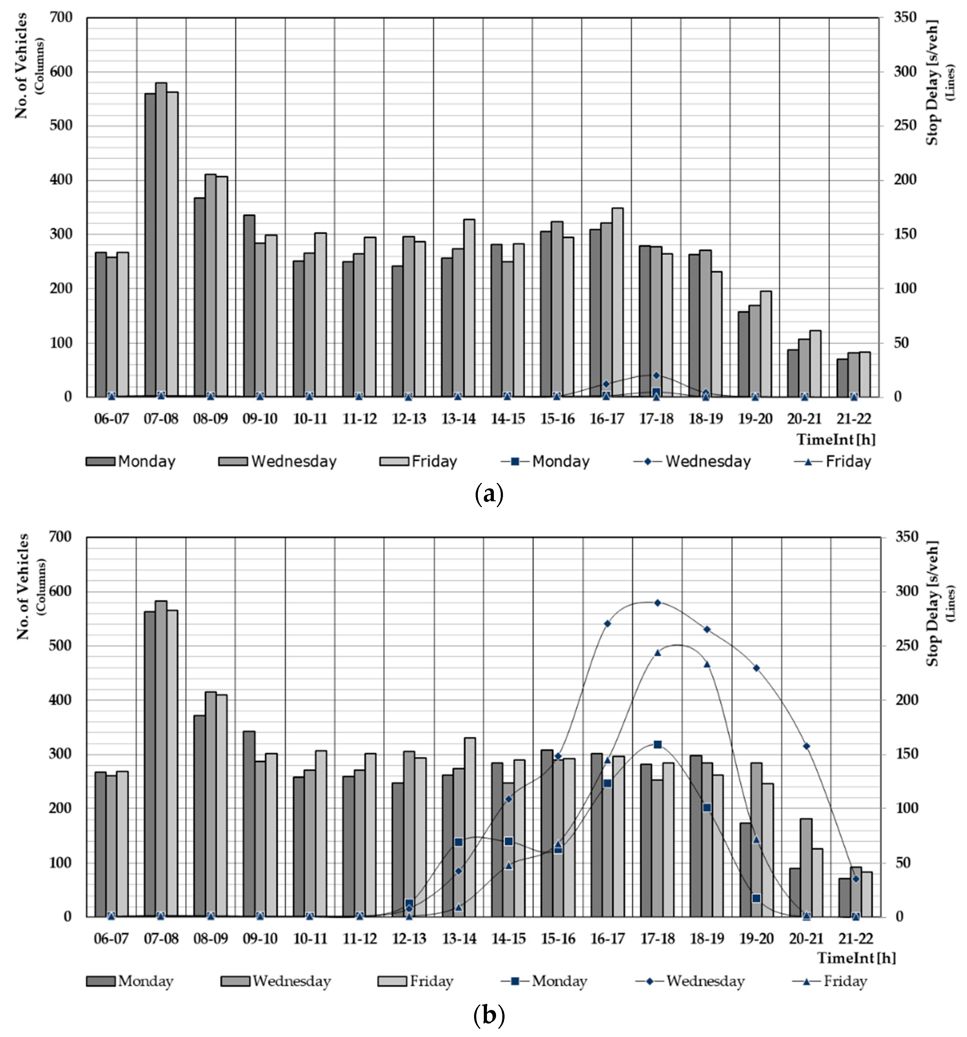
Figure 6a,b show traffic volumes obtained for characteristic weekdays from two detectors. According to these records, peak-hour flows were identified. Figure 6a shows results from detector MQ04P which counts vehicles entering by approaching the road to CT or making a U-turn. Periods from 16.00–18.00 h have the highest volume of traffic, especially HDVs traffic. Results from the detector MQ01P are shown in Figure 6b. The detector is located on the main city corridor; it measures volumes of traffic bound to the city center and shows the peak volumes during the morning hours when most people from eastern suburban areas travel to the city center.

Therefore, for microsimulation traffic modelling, the peak-hour flows distribution is the most important for traffic performance outputs, which are parameters we defined through the assignment model design.

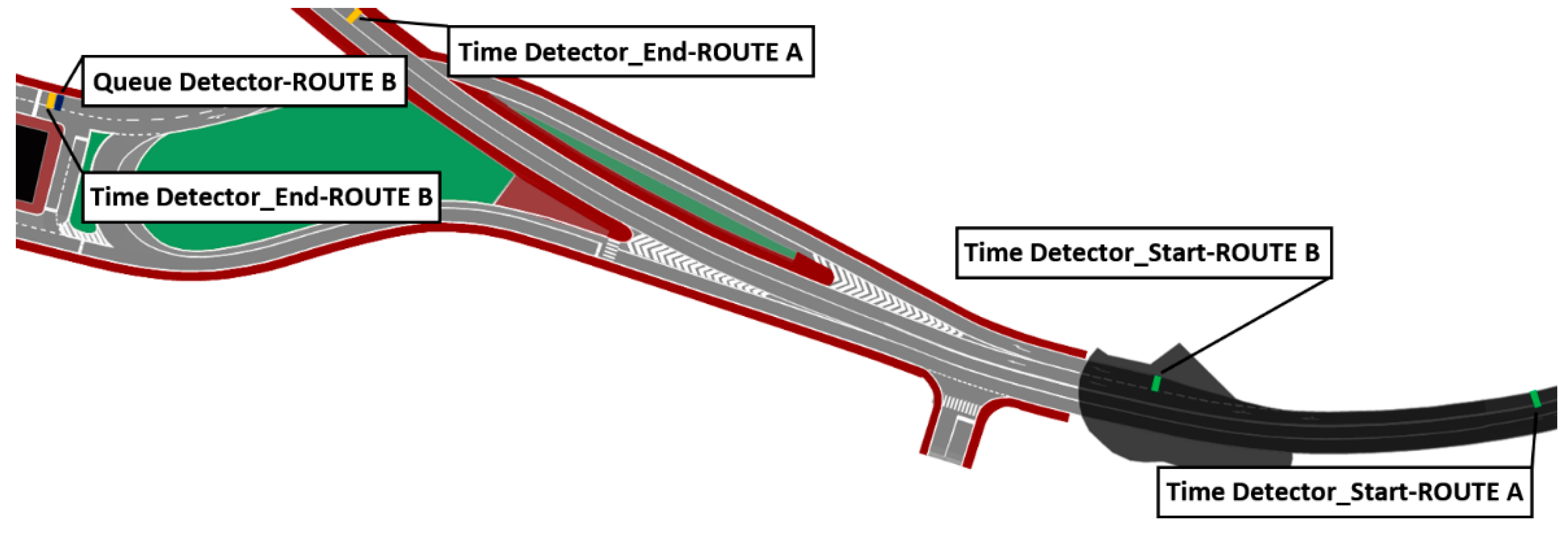
4.3. Model Outputs

The results from the simulation are traffic performance parameters, which we defined through model design. Those parameters are typical for an uninterrupted traffic flow regime and can be used for strategical and tactical traffic management or infrastructure planning. Most of them are derived from three key parameters: flow, density, and speed, with capacity as a critical variable for the road or corridor section. To get the impact on CT traffic in the testing area, we set up three types of Virtual Detectors on the road section and proper lanes depending on traffic directions and route choice: Count detectors, Time detectors (start-stop), and Queue detectors (Figure 7). Time detectors include “start” and “end” virtual objects positioned at the cross-section of lanes heading toward the city center and on approach lane toward CT. Thus, it is possible to obtain the delay in travel time resulting from extensive traffic of HDVs and the limits when it is likely to occur. Queue detectors are set up near the Terminal Gate, where they can measure a backward queue on an approach road (lane). The simulation results are values of the variables or model outputs as follows:

• Number of Vehicles per Vehicle Category (average per lane),
• Queue Length (QLen)-current or average-(in meters),
• Maximum Queue Length (QLenMax)-(in meters),
• Delay Time (DT)-(in seconds, average per vehicle), and
• Stop Delay Time (SDT)-(in seconds, average per vehicle).

The vehicles per Vehicle Category output shows the average number of vehicles for each simulation time step recorded on count detectors. Queue Length represents the distance measured upstream, between the queue detector and the last vehicle in a queue. The current Queue Length is measured with each simulation time step, and the average is calculated for every simulation time interval, in meters. Maximum Queue Length is the variable that describes the maximum queue length measured in every simulation time interval. Delay Time is a variable that measures differences between theoretical and actual obtained travel time of all vehicles in the network. Theoretical travel time is free-flow travel time, and it can be achieved if there are no other vehicles, signal groups, public transport stops, etc. in the network. Stop Delay Time implies average delay per vehicle caused by vehicle retentions in-network for each simulation time step, measured in seconds per vehicle.

4.4. Simulation Settings and Model Validation

Simulation settings include an arrangement of the following attributes: Simulation Time Period, Number of Runs, Random Simulation Seed, and Random Seed Increment for every simulation process based on characteristic weekdays. The simulation period is set at 64,800 s (18 h) where the first and last 3600 s are heat-up and cool-down time periods. Therefore, the active simulation time is 57,600 s or 16 h. Traffic simulations were run independently ten times for every day with different random seeds (27.0, 48.0, and 68.0), where random distributions of vehicle arrivals were generated. For each successive run, a random seed was increased by 1.0. Results are obtained for each vessel category in time-intervals of 1 h.

Model validation can be provided by determining mean absolute deviation, root-mean-square error (RMSE), coefficient of determination, GEH statistic, etc. [26]. Researches by [27,28,29] indicate that model validation using GEH Statistics is one of the most used and generally accepted methods. GEH statistic method of validation is based on a comparison of traffic volumes between simulation and observation [28]. The expression for GEH is [30].

$$GEH=\sqrt{\frac{{\left(VO{L}_{obs}-VO{L}_{sim}\right)}^2}{\frac{VO{L}_{obs}+VO{L}_{sim}}{2}}}$$

(1)

VOL_obs and VOL_sim indicate traffic volumes from the observation and the simulation for every time interval. According to [26,28], 85% GEH values must be less than 5.0 in order to consider a good match between the modeled and observed traffic volumes. The GEH statistic values obtained from (1) are shown in

Table 1. Calculated GEH Statistic Values.

Time Intervals	MQ04PMon	MQ04PWed	MQ04PFri	MQ01PMon	MQ01PWed	MQ01PFri
06–07	0.70	0.68	0.61	0.32	0.26	0.13
07–08	0.30	0.26	0.27	0.00	0.09	0.04
08–09	0.00	0.14	0.13	0.28	0.16	0.16
09–10	0.14	0.00	0.17	0.30	0.32	0.25
10–11	0.13	0.29	0.27	0.51	0.34	0.32
11–12	0.15	0.30	0.25	0.63	0.69	0.67
12–13	0.13	0.26	0.26	0.52	0.72	0.73
13–14	0.00	0.00	0.12	0.57	0.48	0.51
14–15	0.00	0.14	0.37	0.56	0.58	0.27
15–16	0.24	0.24	0.00	0.59	0.57	0.82
16–17	0.35	0.43	0.19	0.59	0.26	0.39
17–18	0.48	0.60	0.25	0.35	0.56	0.43
18–19	0.24	0.34	0.51	0.36	0.29	0.00
19–20	0.17	0.00	0.41	0.27	0.00	0.08
20–21	0.00	0.18	0.00	0.25	0.11	0.21
21–22	0.00	0.45	0.00	0.14	0.38	0.38

.

Comparing the initial test dataset on vehicle volumes (observed data) and simulated vehicle volumes data using Equation (1), no significant deviations were recorded, i.e., GEH Statistic values greater than 5.0, which confirms that the model shows the initial state of traffic flows representatively (Table 1).

4.5. Demand Scenario Management

The purpose of the scenario management is to test the system performance on different occasions depending on the growing demand for container transport and functional requirements for CT operations and to determine the critical values of outputs when system overcapacity occurs. The idea was to transpose the peak-hour traffic demand on typical weekdays for the initial year into future traffic flows with an increase in CT traffic. Thus, the basic demand scenario describes the current situation with CT throughput of around 300,000 TEU/year. For the future demand scenario, we assume an annual growth rate of container transport of 6% per year, which means around 400,000 TEU/year after the 5-year period (

Table 2. Demand Scenario setup.

Demand Scenario	CT Throughput (TEU/Year)	TGT (in seconds)
		HDV Full		HDV Empty
		Aver. Time	St. Dev.	Aver. Time	St. Dev.
Basic Demand scenario	300,000	120.0	30.0	30.0	10.0
Future Demand scenario	400,000	No change		No change

). Considering HDVs traffic demand, the basic demand scenario describes current traffic volumes and time distribution according to measured and validated data. Considering a 5-year scenario, we calculated the correlation between terminal throughput, modal split, and the number of HDVs from 10-year monthly records. Based on this, initial volumes are increased for each time-period for 14.2% on average for HDVs heading to CT (only on Route B). Therefore, the following assumptions are taken in future demand scenario management:

• The annual growth rate in container traffic of 6%
• No significant change in modal split
• No change in peak-hour and typical weekday distributions
• No change in traffic demand for non-CT-bound traffic
• Normal distribution of Terminal Gate waiting time, without a change in future

We assumed normal distribution and no change in waiting time and Terminal Gate control over a long period. However, different waiting times are associated with HDVs with full load containers and for HDVs with empty containers. Usually, security checks for empties are much faster, so HDVs spend much less time at gate control. In this case, it should be noted that having more Terminal Gates is no real option, so we didn’t consider a redesign of the entrance and approach lanes to CT. That was outside of the scope of our research. We just focused on methods for model design and the appropriate adjustment of parameters to observe the potential impact on traffic performances. Considering that, we made some changes in Terminal Gate waiting time for sensitivity test purposes, and we discussed that in the following chapter.

5. Results

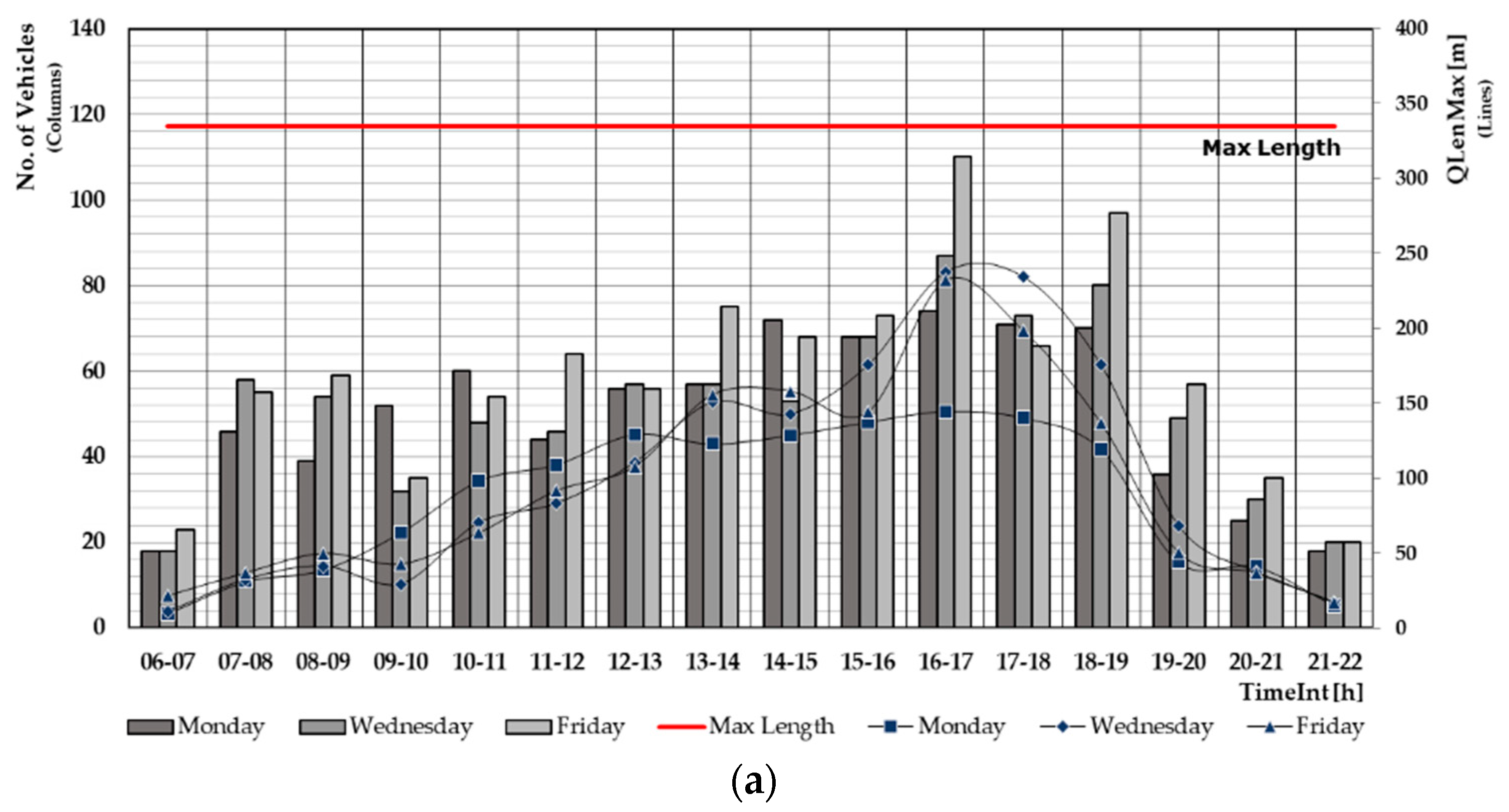
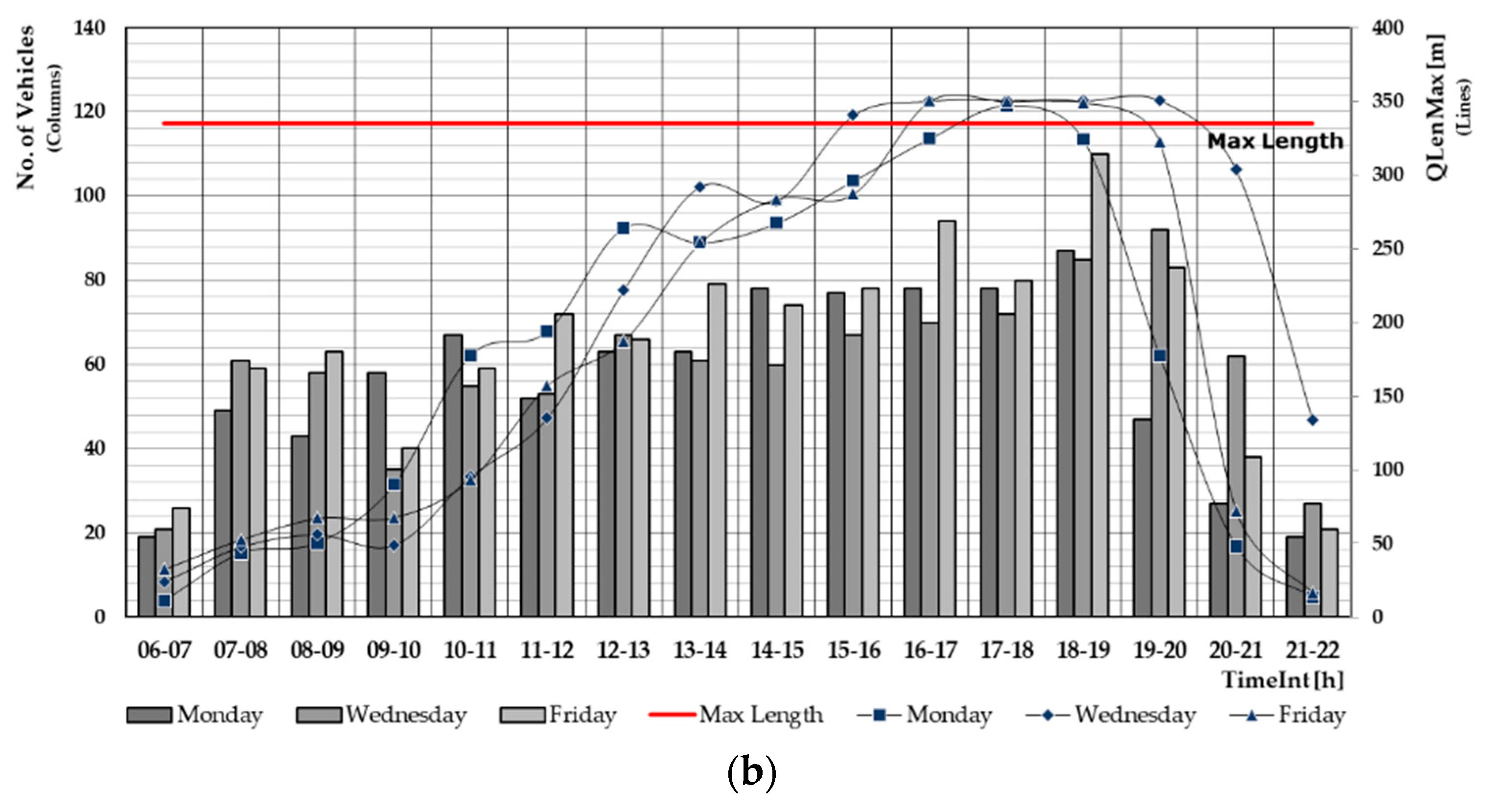
We compared results for two given demand scenarios, basic and future, considering outputs of the most significant variables for measuring traffic performance on selected routes. We observed Queue Length on the approaching road to CT and Delay in travel time on the route toward the city center.

Figure 8 and Figure 9 show traffic situations on the approaching road or Route B, where the queue forms during peak hours. This queue is the most significant in the future demand scenario due to the increased number of HDVs given the higher terminal throughput. In some cases, Maximum Queue Length exceeds the traffic lane’s length, causing congestion and blockage of traffic. That situation was observed several times on Mondays (three times between 15–20 h), on Wednesdays (five times between 15–20 h), and on Fridays (three times on intervals between 16–19 h). In all cases, the Maximum Queue Length was over the length of the approaching road, which is 335 m. It should be noted that total traffic volume and the number of vehicles in Figure 7 and Figure 8 relate to all vehicle classes but include only vehicles after the junction which may turn to CT or make a U-turn back.

The impacts of such long queues are shown in Figure 9a,b, where the Stop Delay Time is considered as a measure of time lost during the travel. Accordingly, all vehicles before the junction are affected, but the most significant effect is on the vehicles on Route A, the main corridor for entrance into the city. For the current situation (basic demand scenario), there is no significant time loss caused by congestion, and only a minor delay can be observed, which in some cases overlaps with terminal peak-hours traffic. However, for the future demand scenario, there is a high increase in delay during the same period. The cause of such a condition is not only the increase in traffic flow during peak-hours but also an overly long queue on the connecting road heading to CT. That can be concluded from simulation runs and post-simulation results.

Therefore, we can conclude that this situation may lead to severe congestion in the future if nothing changes. The change of road and junction geometry is not an option, and the creation of some buffer zone upstream eventually is not likely either. It is reasonable to consider that the reduction of waiting time at the Terminal Gate may cut down the backward queue and consequently neutralize the impact on travel delay on the main city corridor.

The same model can be used to simulate such conditions and make a sensitivity analysis of the traffic system performance if average TGT changes. The initial value of average TGT is 120 s and 30 s, depending on the type of containers loaded to HDV. The normal distribution of time is applied with a standard deviation of 30 s and 10 s. We tested the sensitivity by changing the TGT in a relative decrement of initial time distribution by 10% (

Table 3. Variations in TGT.

TGT Decrement	TGT
	HDVs Full		HDVs Empty
	Aver. Time	St. Dev	Aver. Time	St. Dev
Initial value	120.0	30.0	30.0	10.0
Variation 1	108.0	27.0	30.0	10.0
Variation 2	97.2	24.3	30.0	10.0
Variation 3	87.5	21.9	30.0	10.0
Variation 4	78.7	19.7	30.0	10.0

) and created four variations of the initial TGT values. Note that there is no change in average time for empty loads because of much lower initial values and negligible impact on queue length.

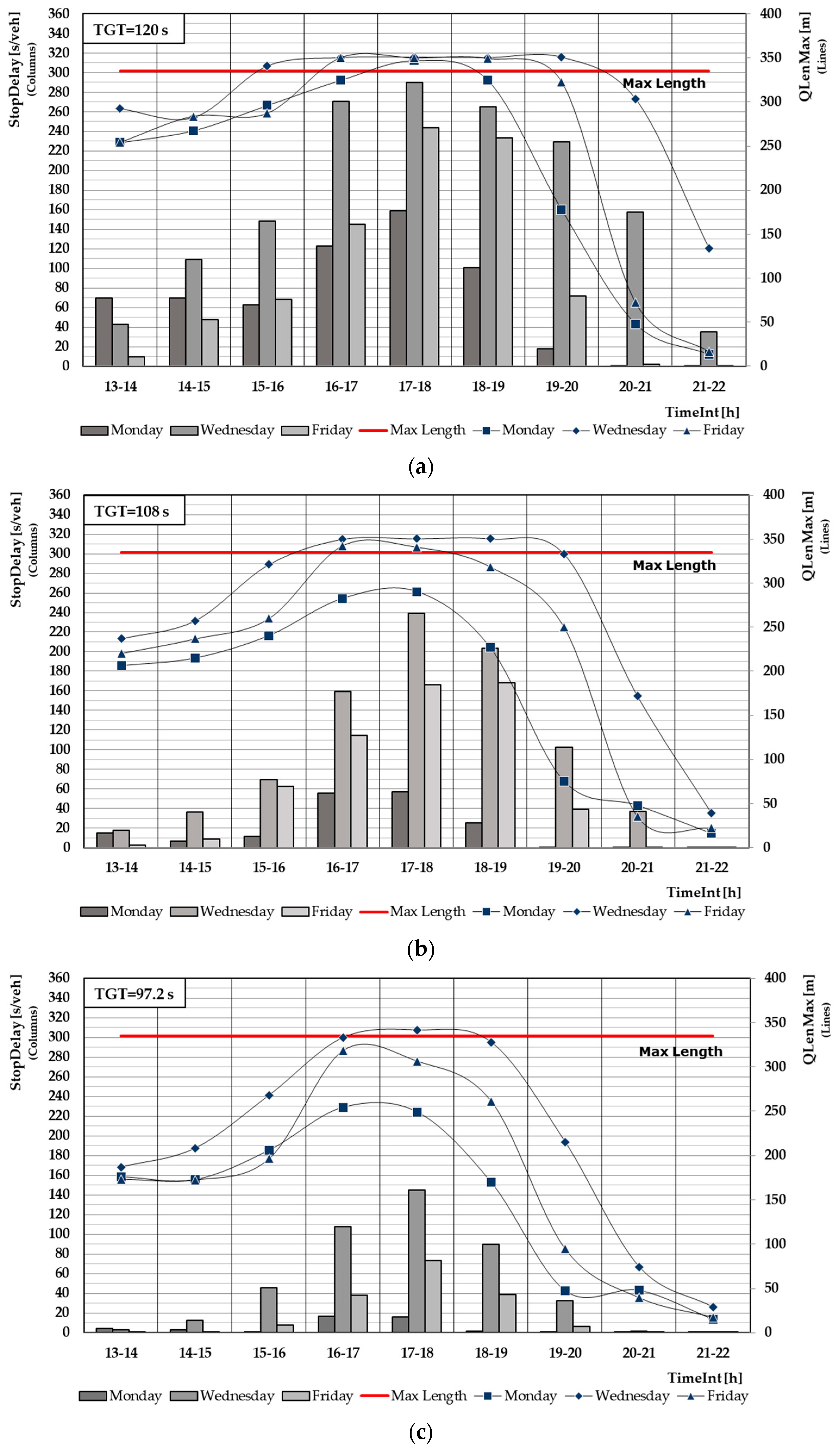
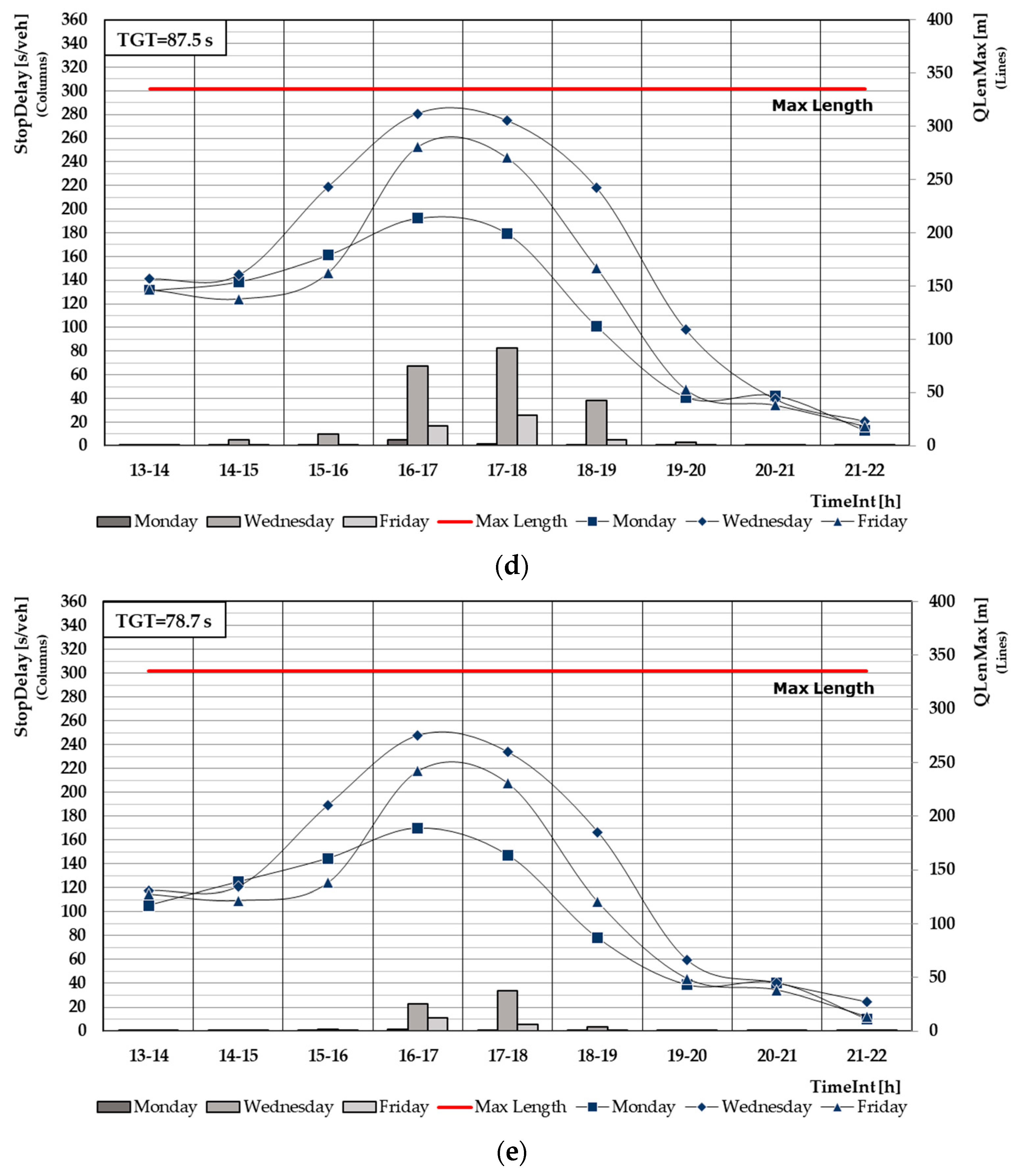
After re-running simulations with variable inputs, we got the new values of Maximum Queue Length and Stop Delay outputs in a changed environment. The results are presented in Figure 10a–e. It can be spotted that maximum recorded values of Stop Delay and the values of Maximum Queue Length coincide in each selected date. Due to the high values of Queue Length above the red line border, the stop of the flow occurs more often, resulting in significant delays if initial values of TGT are applied. After the first variation (10% less time on the gate), Stop Delay is reduced, but the value is still between 160 and 240 s on average per vehicle, recorded on Wednesday. Each subsequent variation shows a decrease of Queue Length and Stop Delays, but variations 3 and 4 assure Queue Length below the red border and practically very rare delays caused by stalled traffic flow. However, that is only a theoretic view on problem-solving. Feasibility of such a reduction in gate control time is doubtful, and it would require additional tests, including in-terminal flow analytics and impacts of terminal capacity constraints.

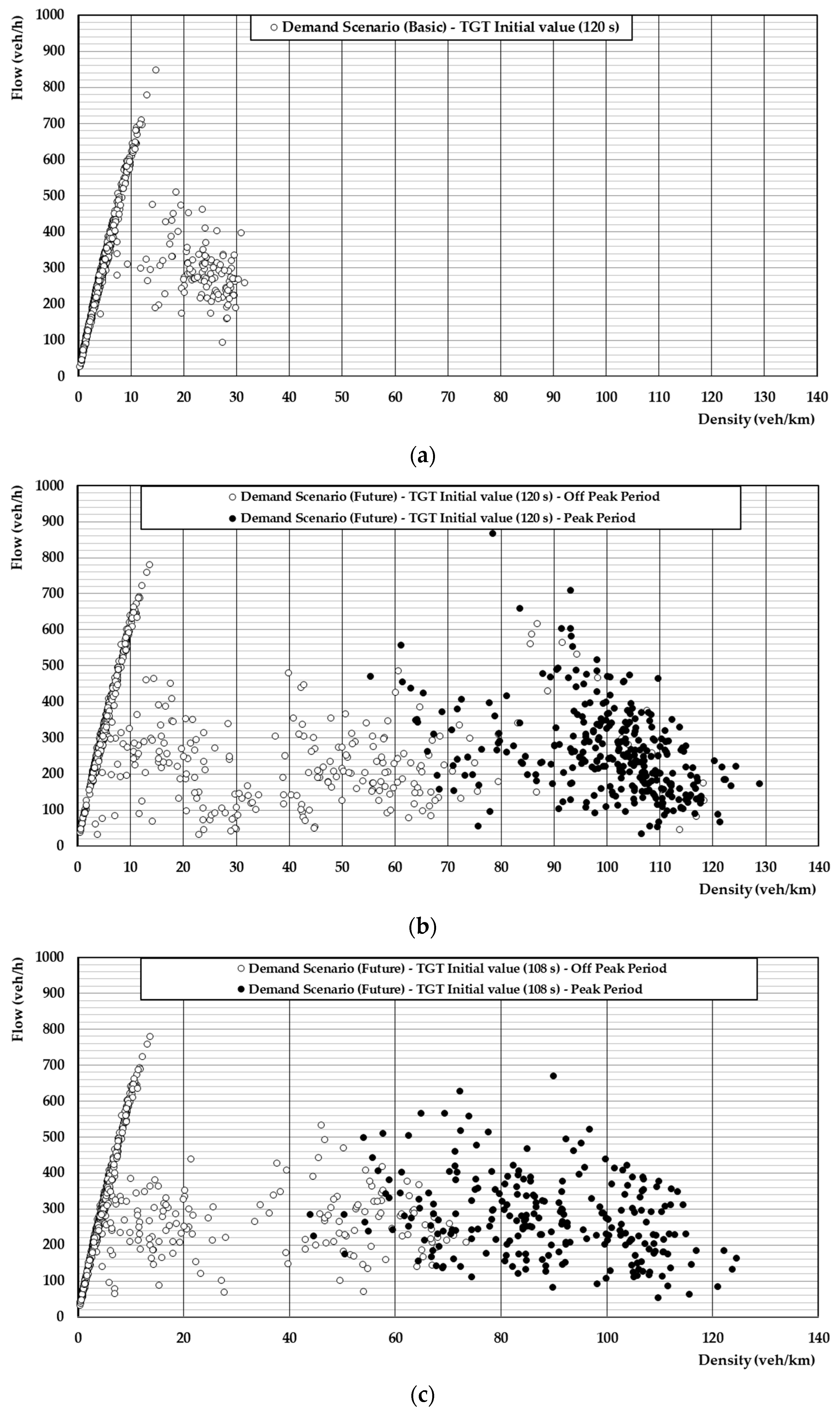
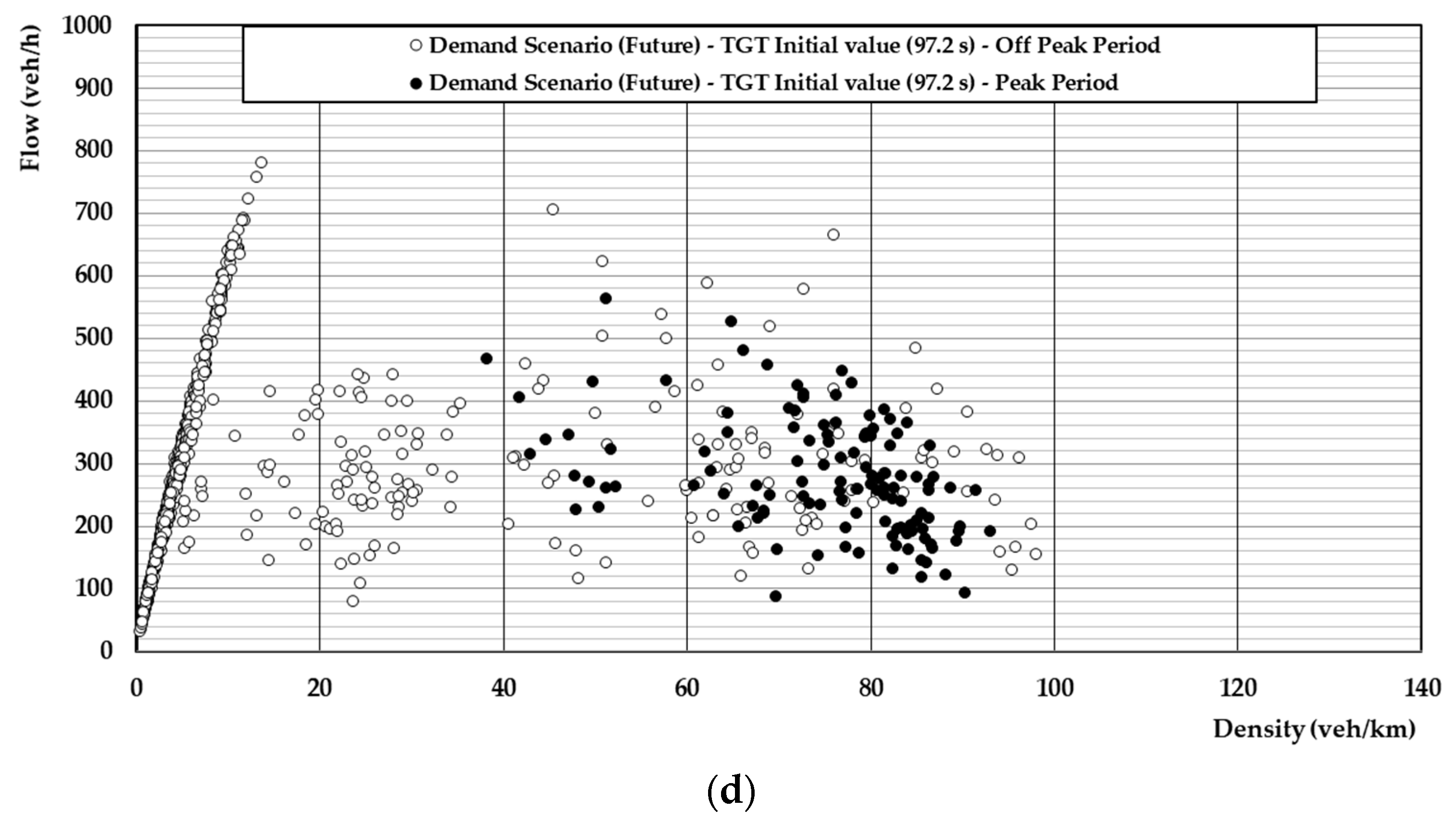
It is interesting to observe the traffic situation on the main link of the network on the route A heading to the city center using the fundamental traffic flow diagram or the Flow-Density diagram. We took data from the link segments for the lane reserved for westbound traffic and counted by the detector located before the junction with the exit lane bound CT. That is the part of the network that is most affected by congestion on the access road to the CT. Figure 11 shows traffic flow and density values in different demand scenarios and variations in TGT. The significant degradation in traffic flow can be observed in case of increased transport demand on CT, especially during peak hours where the traffic condition switches toward the unstable area of the diagram. Changing the TGT policy may contribute to a reduction in congestion but eliminate the effects on traffic flow during the peak periods.

6. Discussion and Conclusions

Proximity to container terminals and the urban area may lead to dysfunction of traffic and significant congestion on the main traffic routes, causing queues, delays in travel time, low levels of services, fuel consumption, and extra vehicle emissions. In this paper, we have proposed a microscopic traffic simulation model for urban networks along container terminals to test the functionality and performance limits of the traffic system. Taking the case study of CT in the port of Rijeka (Croatia) into account, we presented a model design consisting of supply, demand, and control layers to test future scenario development and justify possible impacts on traffic performances. We showed that positive changes in CT transport demand might lead to severe problems in transit traffic flows if current operational conditions persist. The simulations performed illuminated the correlation and impact between system components and outputs. In this case, especially, the correlation between travel time delays and queue length on approaching lanes leads to congestion that may occur in critical weekdays and peak-hour periods if the demand scenario is realized. Some improvements in the Terminal Gate control procedure may lead to a reduction in the waiting time of HDVs entering CT, consequent to shorter queue length. The sensitivity test performed through the simulation model shows the results for several variations in TGT and evaluates effects on traffic delay. This approach may compel decision-makers to take the proper measures well before problems occur or to test the feasibility of new solutions in the future. The microsimulation method we applied here can be used for justification of impacts of present and future port traffic demand on urban traffic performances, evaluation of junctions design in the front of container terminals, or analysis of effects of traffic control strategies within traffic management process.

We analyzed only a part of the urban network. To get a wider picture of the impacts of freight transport on urban traffic conditions, an extension of the research area is necessary. In this case, there exist other port areas that could influence the state of urban traffic in the city. For a comprehensive analysis of those impacts, future research could be directed toward the mesoscopic approach and the implementation of the method, such as MFD.