A Hybrid Deep Learning Model and Comparison for Wind Power Forecasting Considering Temporal-Spatial Feature Extraction


Abstract
:1. Introduction
- The inherent intermittency and uncertainty of wind power lead to difficulties in accurate and rapid wind power output forecasting.
- Few research has paid attention to the bidirectional learning feature of Bi-LSTM in the application of wind power forecasting while more research has been focused on LSTM by far.
- To our best knowledge, the hybrid model BiLSTM-CNN has not yet been applied in the application of wind power forecasting along with the two-way time feature learning and spatial feature extraction analysis.
- Comparison and evaluation among various deep learning models (CNN, LSTM, Bi-LSTM) and their hybrid models in wind power forecasting area have not been systematically researched.
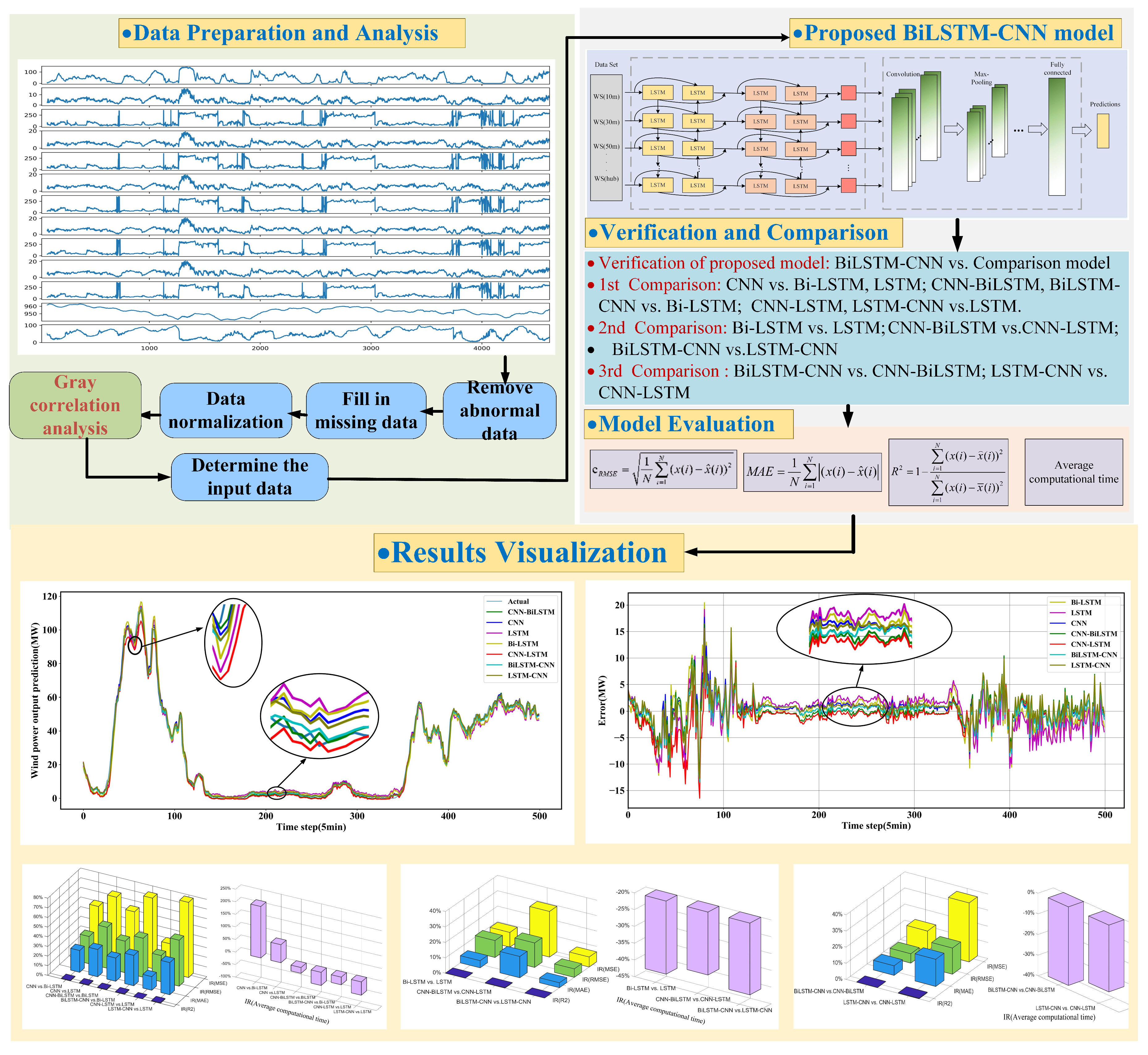
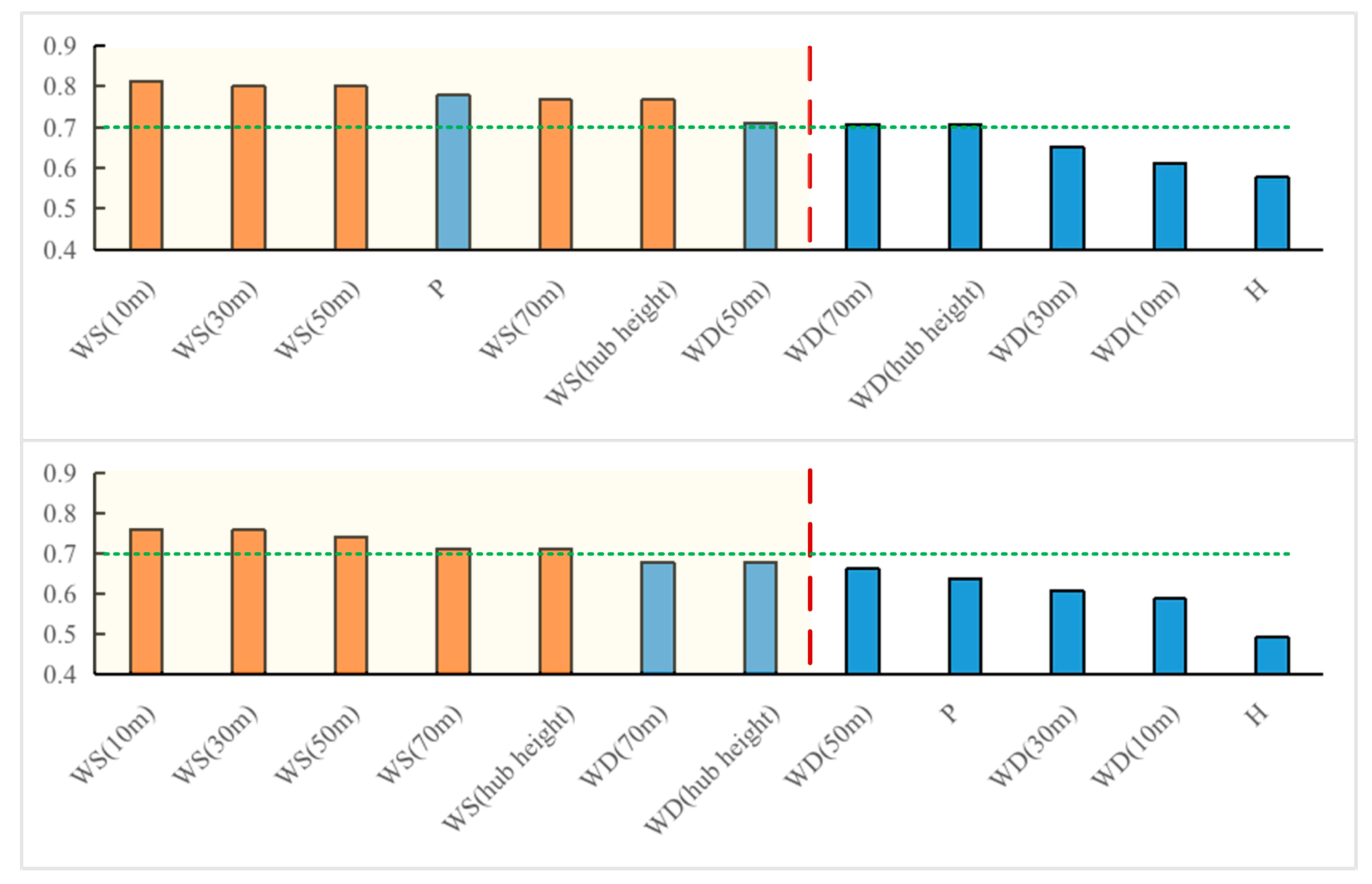
- Through grey correlation analysis under two different normalization methods, multiple wind speed time series data with different heights are selected as inputs of the proposed model. Through this step, the calculation complexity and time are reduced.
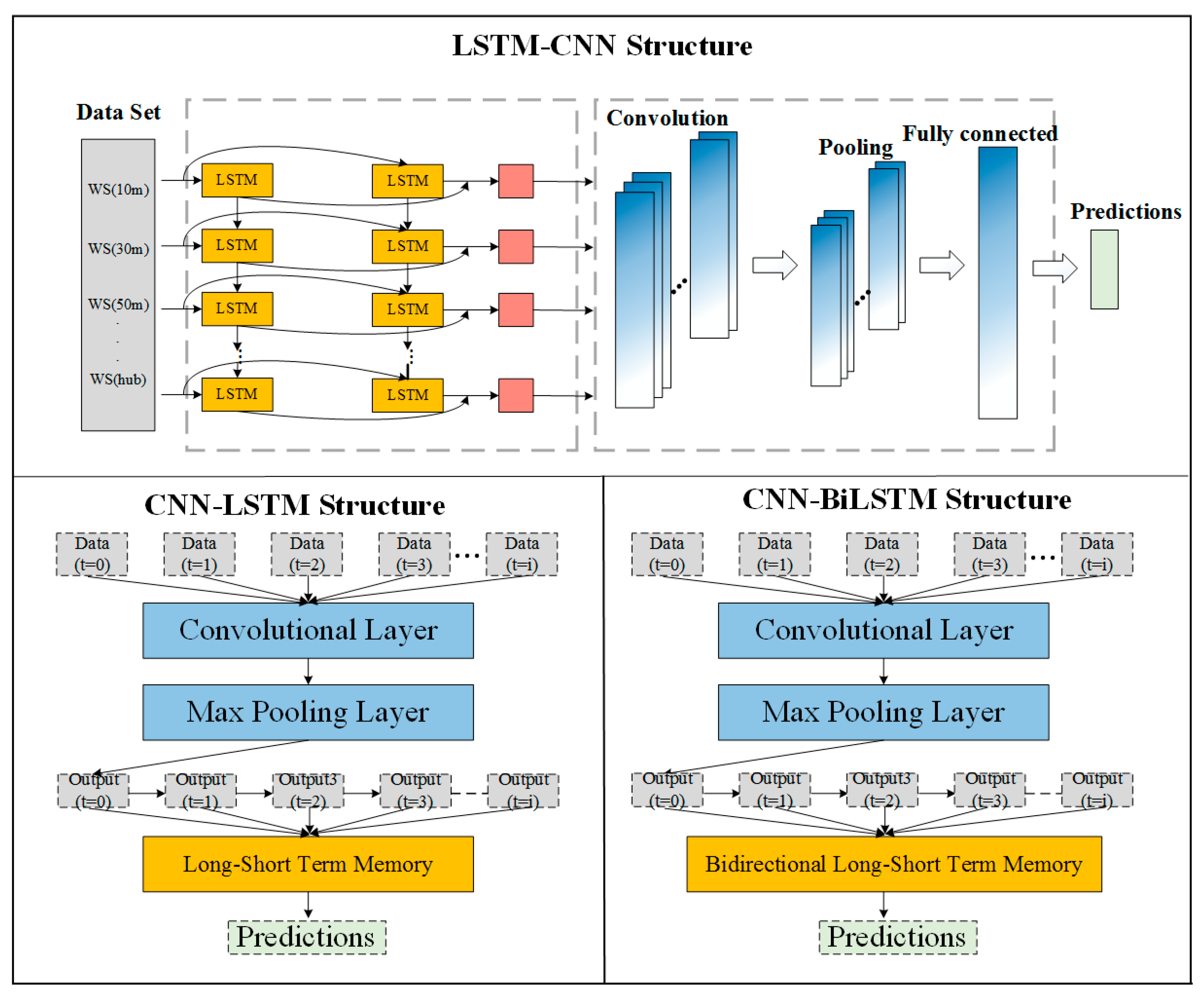
- The BiLSTM-CNN algorithm is innovatively proposed in this research, which can extract time and space features in succession to fully mine the information among the input data and obtain high prediction accuracy. The contribution of this proposed model fills in the research gaps. With the experiment conducted in a real wind farm as a case study, the performance of the proposed model is verified by comparison with other single and hybrid deep learning models.
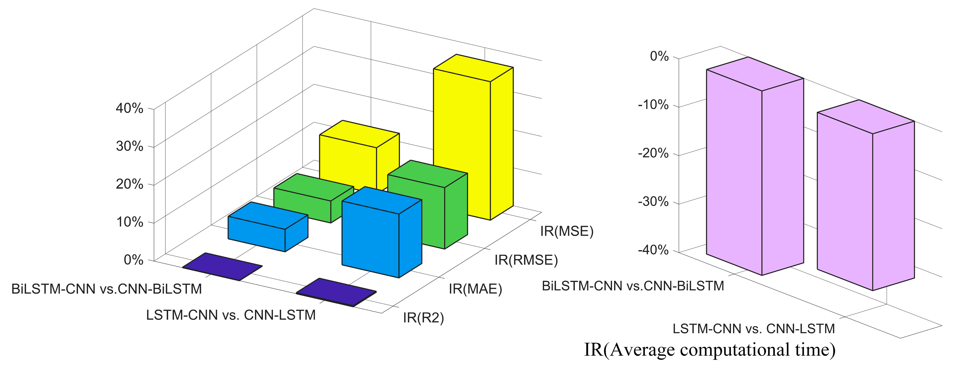
- Model comparison among different deep learning models (LSTM, BiLSTM, CNN, BiLSTM-CNN, LSTM-CNN, CNN-BiLSTM, CNN-LSTM) are systematically studied in wind power forecasting. Three sets of comparison are conducted. Specifically, the role of the introduction of CNN to extract the spatial features among multiple wind speed series with different height is studied; the comparison between Bi-LSTM and LSTM is also studied to verify the significance bidirectional temporal feature extraction ability of Bi-LSTM; Besides, the comparison of BiLSTM-CNN vs. CNN-BiLSTM and LSTM-CNN vs. CNN-LSTM is also experimented to study the preference between ‘‘the temporal characteristics of time series are extracted in the beginning and later the spatial characteristics are extracted’ and ‘the spatial characteristics of time series are extracted in the beginning and later the temporal characteristics are extracted’.
2. Methodology
2.1. Grey Correlation Analysis
2.2. Proposed Hybrid Model
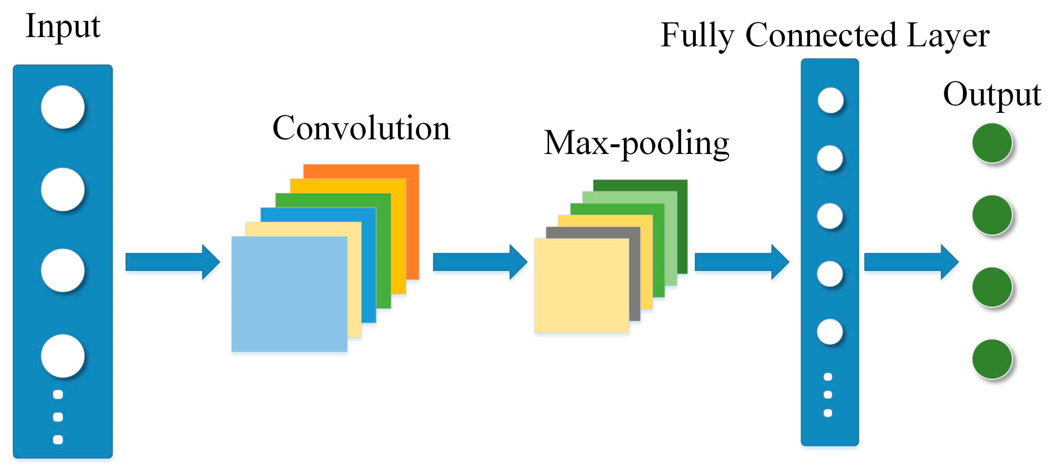
2.2.1. CNN Model
2.2.2. Bi-LSTM Model
- (1)
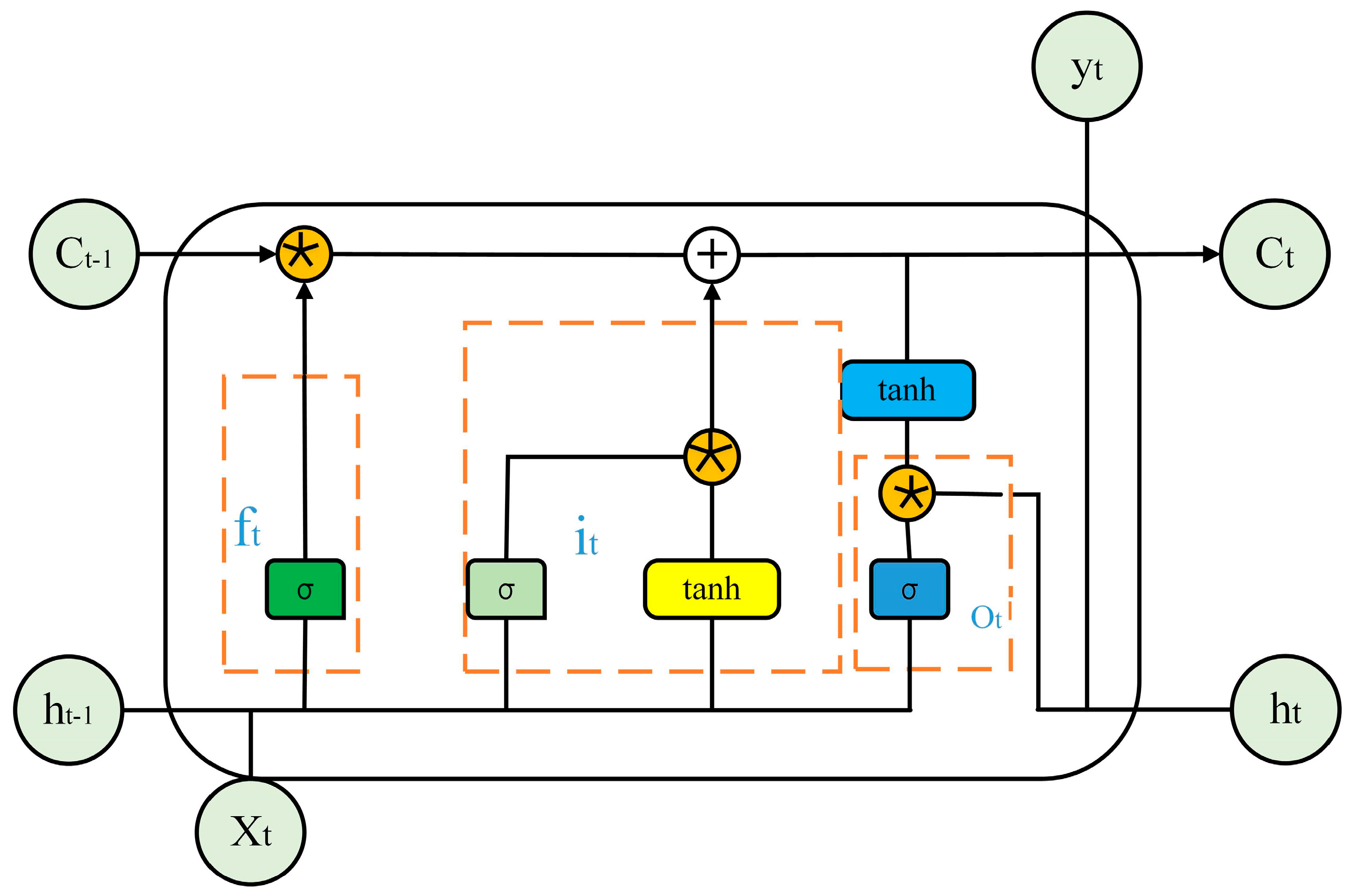
- LSTM Model
- (2)
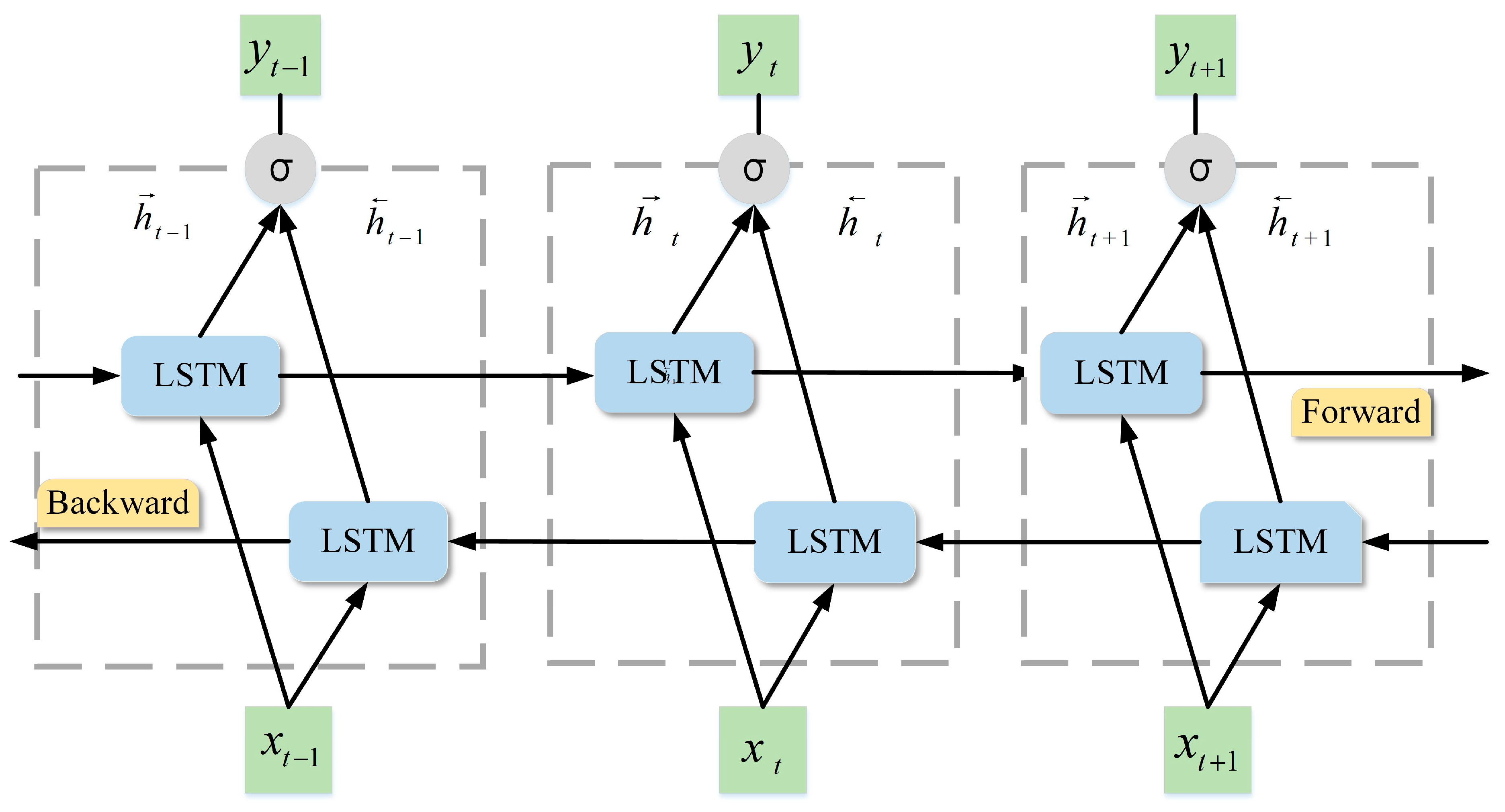
- Bi-LSTM Model
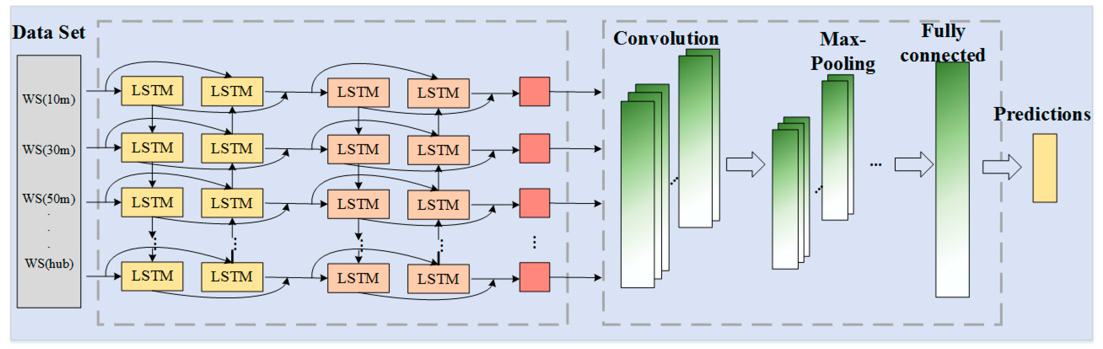
2.2.3. Hybrid Model
3. Case Study
3.1. Data Process and Selection
3.2. Results
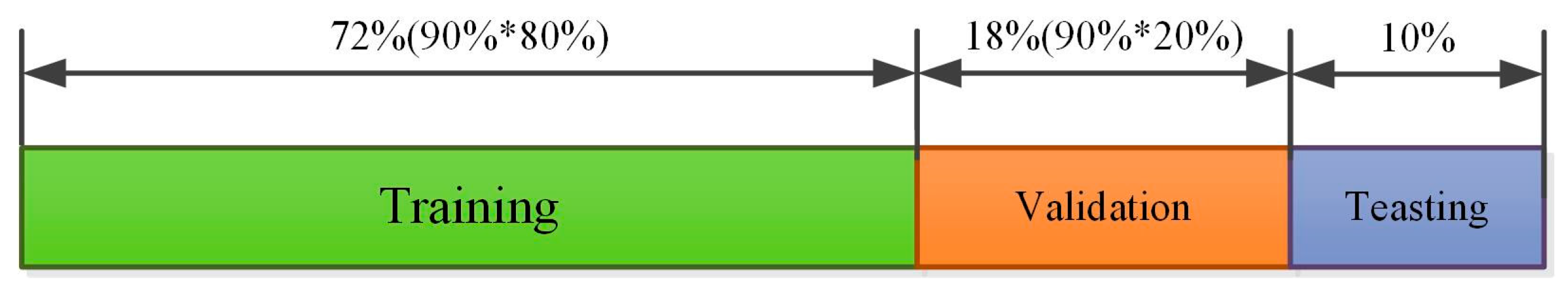
3.2.1. Data Set Division and Evaluation Indicators
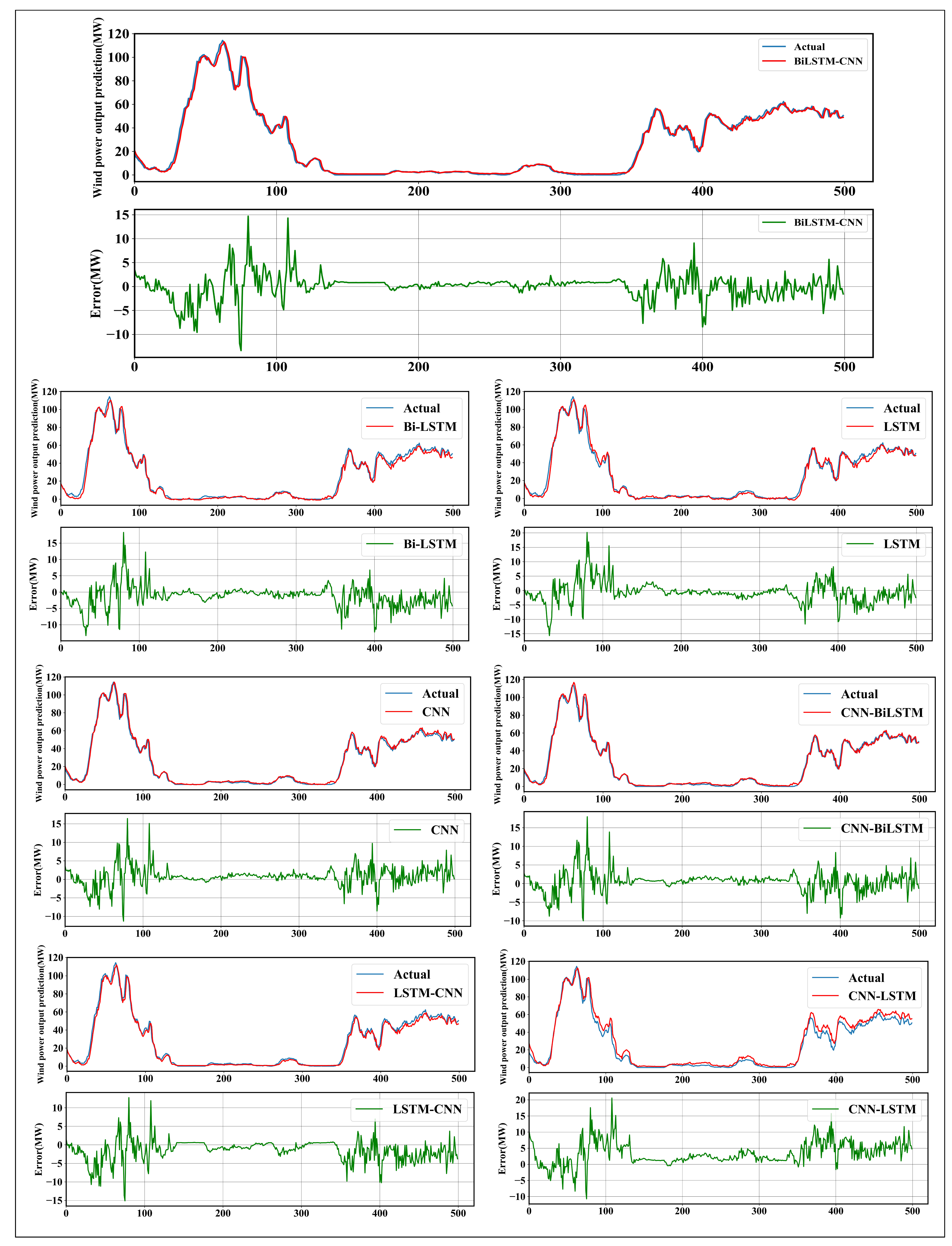
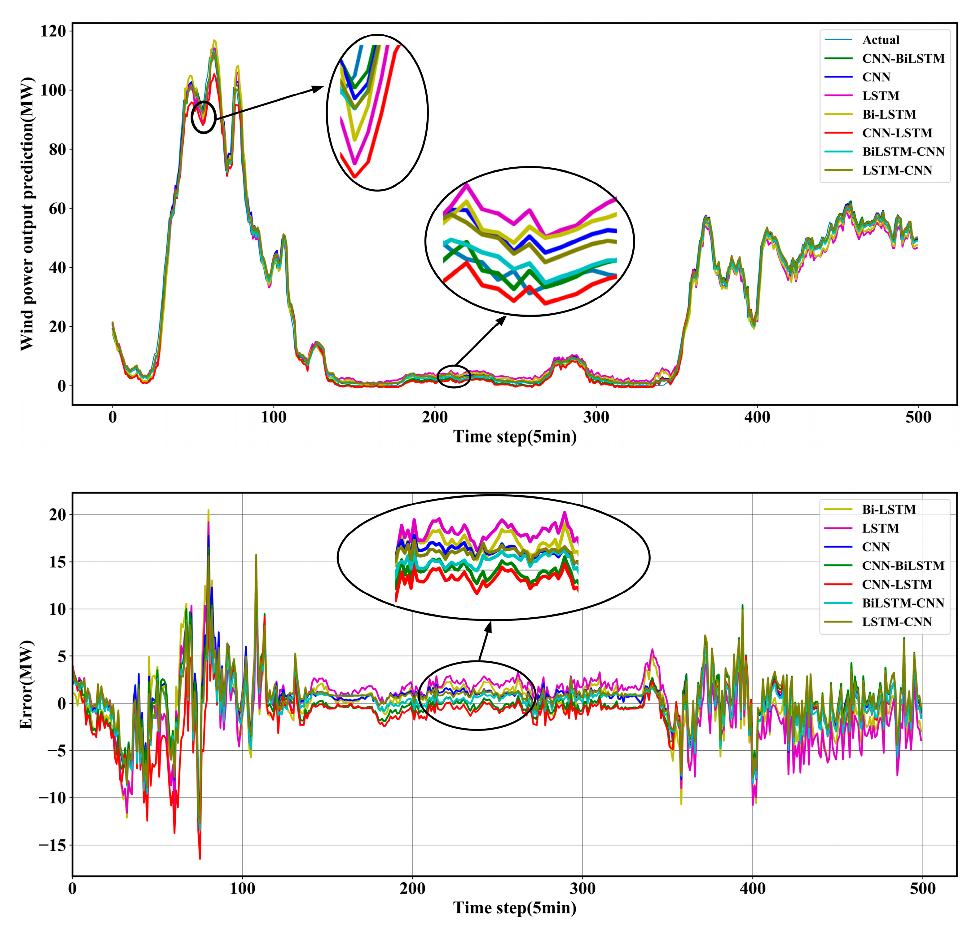
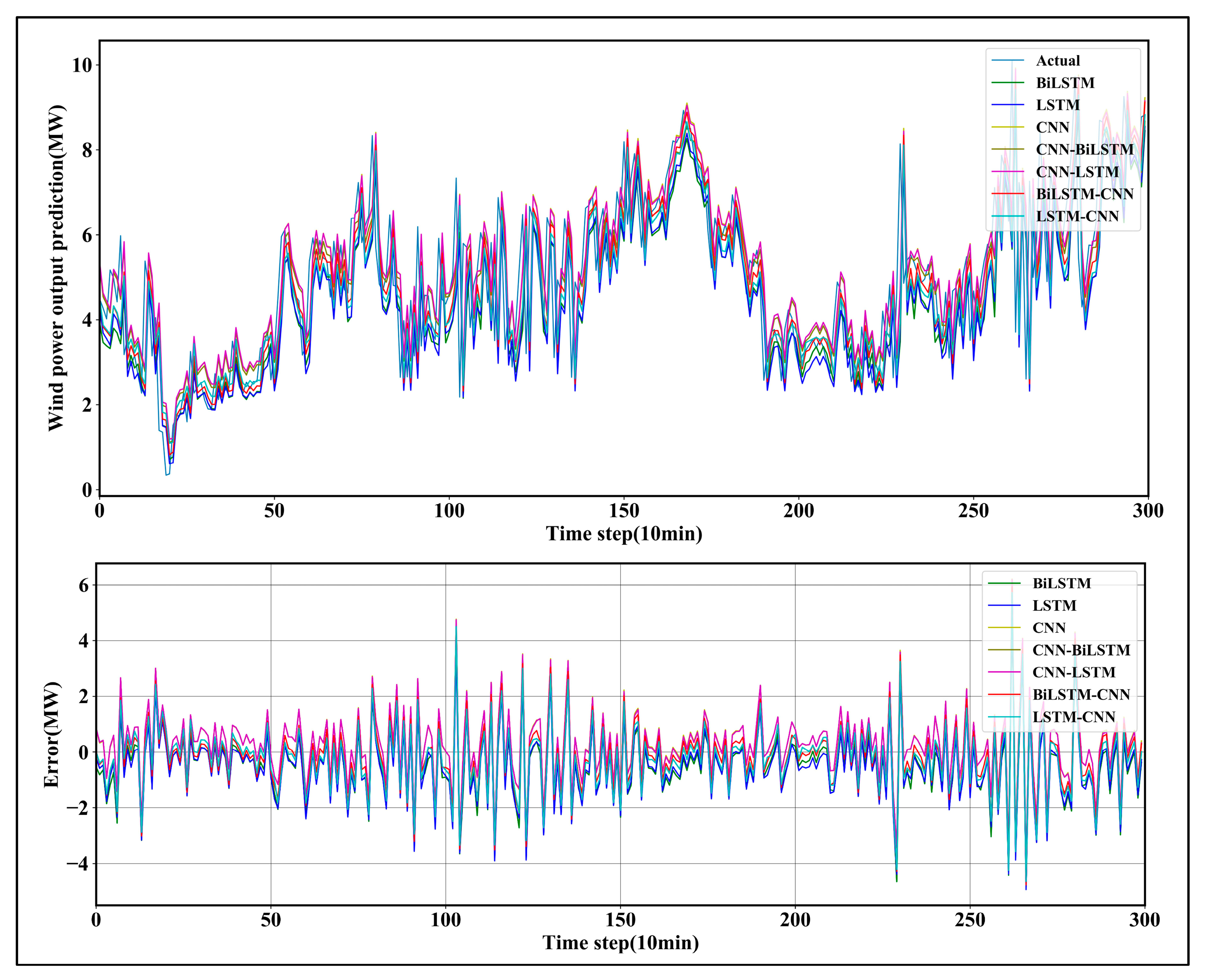
3.2.2. Experiments and Comparison
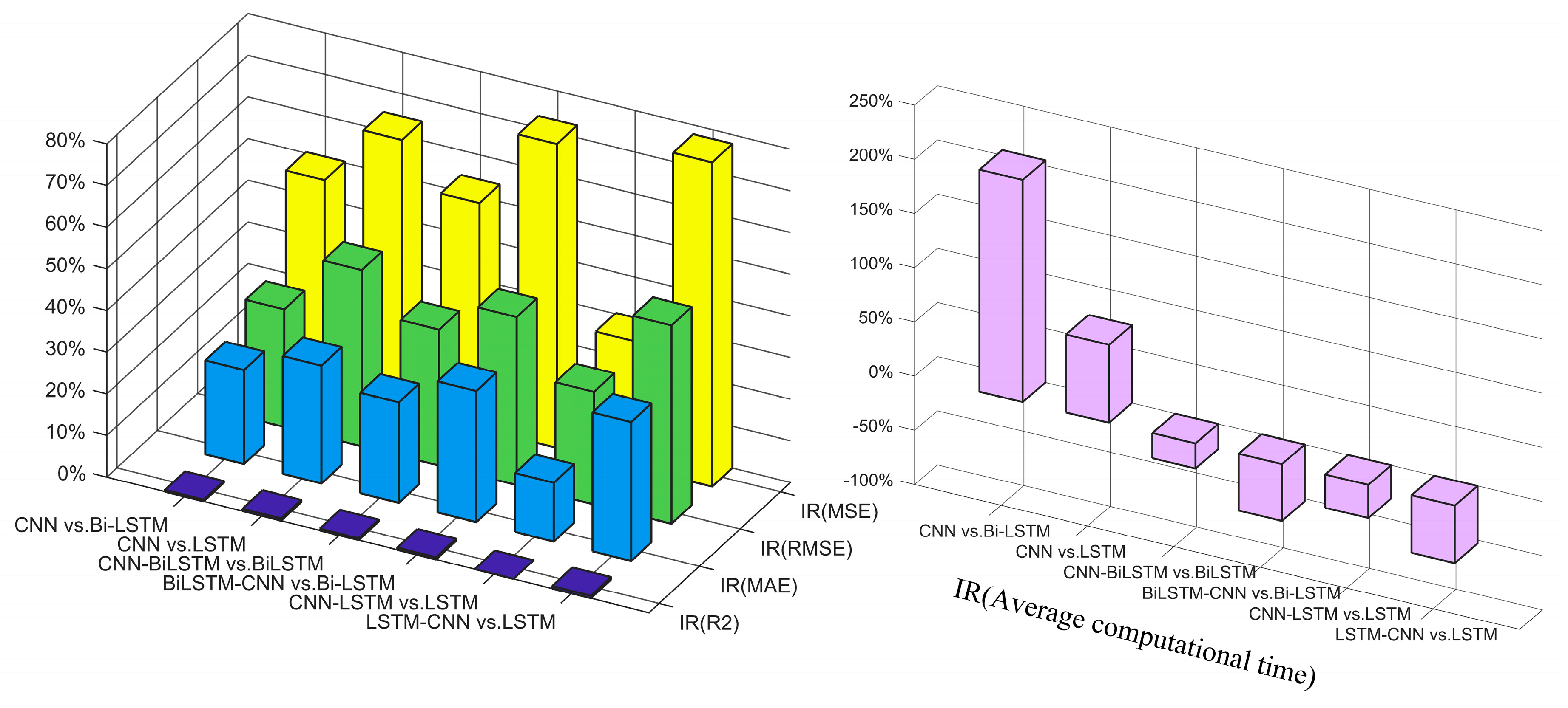
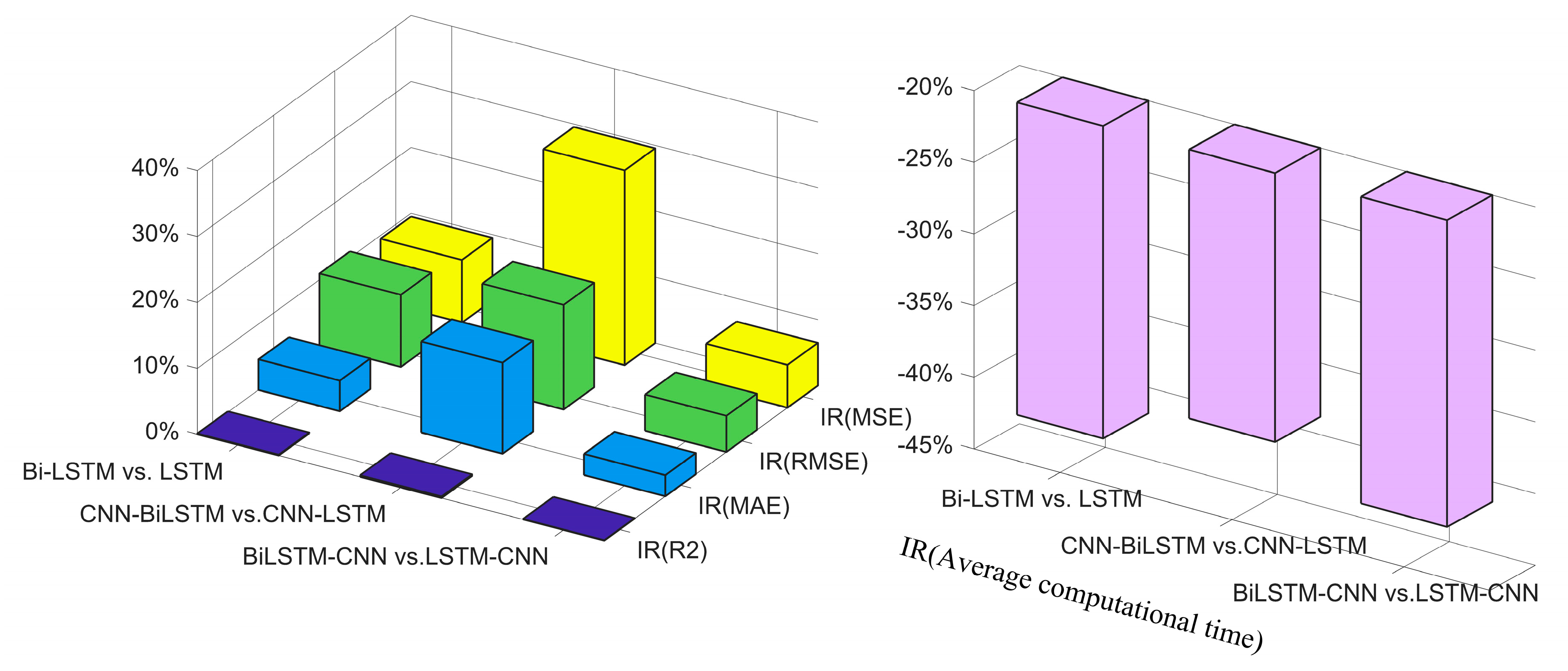
3.2.3. Further Study
4. Conclusions and Discussion
Author Contributions
Funding
Conflicts of Interest
References
- Aly, H.H. A Novel Deep Learning Intelligent Clustered Hybrid Models for Wind Speed and Power Forecasting. Energy 2020, 213, 118773. [Google Scholar] [CrossRef]
- Afshar, K.; Ghiasvand, F.S.; Bigdeli, N. Optimal bidding strategy of wind power producers in pay-as-bid power markets. Renew. Energy 2018, 127, 575–586. [Google Scholar] [CrossRef]
- Global Wind Report 2019|Global Wind Energy Council. Available online: https://gwec.net/global-wind-report-2019/ (accessed on 10 October 2020).
- Naik, J.; Bisoi, R.; Dash, P. Prediction interval forecasting of wind speed and wind power using modes decomposition based low rank multi-kernel ridge regression. Renew. Energy 2018, 129, 357–383. [Google Scholar] [CrossRef]
- Wang, K.; Niu, D.; Sun, L.; Zhen, H.; Liu, J.; De, G.; Xu, X. Wind Power Short-Term Forecasting Hybrid Model Based on CEEMD-SE Method. Processes 2019, 7, 843. [Google Scholar] [CrossRef] [Green Version]
- Lahouar, A.; Slama, J.B.H. Hour-ahead wind power forecast based on random forests. Renew. Energy 2017, 109, 529–541. [Google Scholar] [CrossRef]
- James, E.P.; Benjamin, S.G.; Marquis, M. Offshore wind speed estimates from a high-resolution rapidly updating numerical weather prediction model forecast dataset. Wind Energy 2018, 21, 264–284. [Google Scholar] [CrossRef]
- Zuluaga, C.D.; Alvarez, M.A.; Giraldo, E. Short-term wind speed prediction based on robust Kalman filtering: An experimental comparison. Appl. Energy 2015, 156, 321–330. [Google Scholar] [CrossRef]
- Torres, J.L.; Garcia, A.; De Blas, M.; De Francisco, A. Forecast of hourly average wind speed with ARMA models in Navarre (Spain). Sol. Energy 2005, 79, 65–77. [Google Scholar] [CrossRef]
- Sfetsos, A. A novel approach for the forecasting of mean hourly wind speed time series. Renew. Energy 2002, 27, 163–174. [Google Scholar] [CrossRef]
- Cadenas, E.; Jaramillo, O.A.; Rivera, W. Analysis and forecasting of wind velocity in chetumal, quintana roo, using the single exponential smoothing method. Renew. Energy 2010, 35, 925–930. [Google Scholar] [CrossRef]
- Samet, H.; Marzbani, F. Quantizing the deterministic nonlinearity in wind speed time series. Renew. Sustain. Energy Rev. 2014, 39, 1143–1154. [Google Scholar] [CrossRef]
- Ouyang, T.; Zha, X.; Qin, L. A combined multivariate model for wind power prediction. Energy Convers. Manag. 2017, 144, 361–373. [Google Scholar] [CrossRef]
- Marugán, A.P.; Márquez, F.P.G.; Perez, J.M.P.; Ruiz-Hernández, D. A survey of artificial neural network in wind energy systems. Appl. Energy 2018, 228, 1822–1836. [Google Scholar] [CrossRef] [Green Version]
- Barman, M.; Choudhury, N.B.D. Season specific approach for short-term load forecasting based on hybrid FA-SVM and similarity concept. Energy 2019, 174, 886–896. [Google Scholar] [CrossRef]
- Tso, G.K.; Yau, K.K. Predicting electricity energy consumption: A comparison of regression analysis, decision tree and neural networks. Energy 2007, 32, 1761–1768. [Google Scholar] [CrossRef]
- Voyant, C.; Notton, G.; Kalogirou, S.; Nivet, M.-L.; Paoli, C.; Motte, F.; Fouilloy, A. Machine learning methods for solar radiation forecasting: A review. Renew. Energy 2017, 105, 569–582. [Google Scholar] [CrossRef]
- Li, L.-L.; Zhao, X.; Tseng, M.-L.; Tan, R.R. Short-term wind power forecasting based on support vector machine with improved dragonfly algorithm. J. Clean. Prod. 2020, 242, 118447. [Google Scholar] [CrossRef]
- Liu, M.; Cao, Z.; Zhang, J.; Wang, L.; Huang, C.; Luo, X. Short-term wind speed forecasting based on the Jaya-SVM model. Int. J. Electr. Power Energy Syst. 2020, 121, 106056. [Google Scholar] [CrossRef]
- Wang, G.; Jia, R.; Liu, J.; Zhang, H. A hybrid wind power forecasting approach based on Bayesian model averaging and ensemble learning. Renew. Energy 2020, 145, 2426–2434. [Google Scholar] [CrossRef]
- Rodríguez, F.; Florez-Tapia, A.M.; Fontán, L.; Galarza, A. Very short-term wind power density forecasting through artificial neural networks for microgrid control. Renew. Energy 2020, 145, 1517–1527. [Google Scholar] [CrossRef]
- Hinton, G.E.; Osindero, S.; Teh, Y.-W. A fast learning algorithm for deep belief nets. Neural Comput. 2006, 18, 1527–1554. [Google Scholar] [CrossRef] [PubMed]
- LeCun, Y.; Bottou, L.; Bengio, Y.; Haffner, P. Gradient-based learning applied to document recognition. Proc. IEEE 1998, 86, 2278–2324. [Google Scholar] [CrossRef] [Green Version]
- Hochreiter, S.; Schmidhuber, J. Long short-term memory. Neural Comput. 1997, 9, 1735–1780. [Google Scholar] [CrossRef] [PubMed]
- Goodfellow, I.; Pouget-Abadie, J.; Mirza, M.; Xu, B.; Warde-Farley, D.; Ozair, S.; Courville, A.; Bengio, Y. Generative Adversarial Networks. arXiv 2014, arXiv:1406.2661. [Google Scholar]
- He, K.; Zhang, X.; Ren, S.; Sun, J. Deep residual learning for image recognition. arXiv 2016, arXiv:1512.03385. [Google Scholar]
- Wang, K.; Qi, X.; Liu, H. Photovoltaic power forecasting based LSTM-Convolutional Network. Energy 2019, 189, 116225. [Google Scholar] [CrossRef]
- He, W. Load forecasting via deep neural networks. Procedia Comput. Sci. 2017, 122, 308–314. [Google Scholar] [CrossRef]
- Díaz–Vico, D.; Torres–Barrán, A.; Omari, A.; Dorronsoro, J.R. Deep neural networks for wind and solar energy prediction. Neural Process. Lett. 2017, 46, 829–844. [Google Scholar] [CrossRef]
- Hong, Y.-Y.; Rioflorido, C.L.P.P. A hybrid deep learning-based neural network for 24-h ahead wind power forecasting. Appl. Energy 2019, 250, 530–539. [Google Scholar] [CrossRef]
- Qing, X.; Niu, Y. Hourly day-ahead solar irradiance prediction using weather forecasts by LSTM. Energy 2018, 148, 461–468. [Google Scholar] [CrossRef]
- Gao, M.; Li, J.; Hong, F.; Long, D. Day-ahead power forecasting in a large-scale photovoltaic plant based on weather classification using LSTM. Energy 2019, 187, 115838. [Google Scholar] [CrossRef]
- Cai, M.; Pipattanasomporn, M.; Rahman, S. Day-ahead building-level load forecasts using deep learning vs. traditional time-series techniques. Appl. Energy 2019, 236, 1078–1088. [Google Scholar] [CrossRef]
- Duan, M.; Li, K.; Yang, C.; Li, K. A hybrid deep learning CNN–ELM for age and gender classification. Neurocomputing 2018, 275, 448–461. [Google Scholar] [CrossRef]
- Wang, H.; Yang, Z.; Yu, Q.; Hong, T.; Lin, X. Online reliability time series prediction via convolutional neural network and long short term memory for service-oriented systems. Knowl.-Based Syst. 2018, 159, 132–147. [Google Scholar] [CrossRef]
- Bao, J.; Liu, P.; Ukkusuri, S.V. A spatiotemporal deep learning approach for citywide short-term crash risk prediction with multi-source data. Accid. Anal. Prev. 2019, 122, 239–254. [Google Scholar] [CrossRef] [PubMed]
- Wen, C.; Liu, S.; Yao, X.; Peng, L.; Li, X.; Hu, Y.; Chi, T. A novel spatiotemporal convolutional long short-term neural network for air pollution prediction. Sci. Total Environ. 2019, 654, 1091–1099. [Google Scholar] [CrossRef] [PubMed]
- Liu, H.; Mi, X.; Li, Y. Smart deep learning based wind speed prediction model using wavelet packet decomposition, convolutional neural network and convolutional long short term memory network. Energy Convers. Manag. 2018, 166, 120–131. [Google Scholar] [CrossRef]
- Wang, J.-Z.; Wang, Y.; Jiang, P. The study and application of a novel hybrid forecasting model–A case study of wind speed forecasting in China. Appl. Energy 2015, 143, 472–488. [Google Scholar] [CrossRef]
- Jiang, P.; Wang, Y.; Wang, J. Short-term wind speed forecasting using a hybrid model. Energy 2017, 119, 561–577. [Google Scholar] [CrossRef]
- Gu, J.; Wang, Z.; Kuen, J.; Ma, L.; Shahroudy, A.; Shuai, B.; Liu, T.; Wang, X.; Wang, G.; Cai, J. Recent advances in convolutional neural networks. Pattern Recognit. 2018, 77, 354–377. [Google Scholar] [CrossRef] [Green Version]
- Huang, Y.; Shen, L.; Liu, H. Grey relational analysis, principal component analysis and forecasting of carbon emissions based on long short-term memory in China. J. Clean. Prod. 2019, 209, 415–423. [Google Scholar] [CrossRef]
- Atef, S.; Eltawil, A.B. Assessment of stacked unidirectional and bidirectional long short-term memory networks for electricity load forecasting. Electr. Power Syst. Res. 2020, 187, 106489. [Google Scholar] [CrossRef]


| WP | WS (10 m) | WD (10 m) | WS (30 m) | WD (30 m) | WS (50 m) | WD (50 m) | |
| Count | 4597 | 4597 | 4597 | 4597 | 4597 | 4597 | 4597 |
| Mean | 38.91 | 4.55 | 118.79 | 5.20 | 120.60 | 5.45 | 120.62 |
| Std | 33.81 | 2.35 | 99.14 | 2.69 | 101.10 | 2.80 | 100.66 |
| Min | 0 | 0.13 | 0 | 0.17 | 0 | 0.13 | 0 |
| Max | 143.09 | 15.86 | 360 | 19.15 | 360 | 19.64 | 360 |
| WS (70 m) | WD (70 m) | WS (hub height) | WD (hub height) | Pressure (P) | Humidity (H) | ||
| Count | 4597 | 4597 | 4597 | 4597 | 4597 | 4597 | |
| Mean | 5.62 | 123.32 | 5.62 | 123.32 | 952.98 | 52.251817 | |
| Std | 2.86 | 99.90 | 2.86 | 99.90 | 5.18 | 24.32 | |
| Min | 0.15 | 0 | 0.15 | 0 | 941.34 | 4.01 | |
| Max | 20.75 | 360 | 20.75 | 360 | 963.04 | 99.027 | |
| Standard Method | Grey Correlation Degree and Ranking Sequences | |||||||||||
|---|---|---|---|---|---|---|---|---|---|---|---|---|
| WS (10 m) | WD (10 m) | WS (30 m) | WD (30 m) | WS (50 m) | WD (50 m) | WS (70 m) | WD (70 m) | WS (Hub Height) | WD (Hub Height) | P | H | |
| PDN | 0.811 | 0.610 | 0.800 | 0.652 | 0.800 | 0.710 | 0.767 | 0.708 | 0.767 | 0.708 | 0.778 | 0.577 |
| Ranking: WS (10 m) > WS (30 m) > WS (50 m) > P > WS (70 m) > WS (hub height) > WD (50 m) > WD (70 m) > WD (hub height) > WD (30 m) > WD (10 m) > H | ||||||||||||
| AVN | 0.761 | 0.587 | 0.758 | 0.608 | 0.742 | 0.662 | 0.712 | 0.677 | 0.712 | 0.677 | 0.636 | 0.492 |
| Ranking: WS (10 m) > WS (30 m) > WS (50 m) > WS (70 m) > WS (hub height) > WD (70 m) > WD (hub height) > WD (50 m) > P > WD (30 m) > WD (10 m) > H | ||||||||||||
| Proposed Model | Configuration | |||
|---|---|---|---|---|
| BiLSTM-CNN | Bi-LSTM | Units1 | Units = 64; | Epoch = 80, Batch size = 100; Optimizer = ‘Adam’; Learning rate = 0.001. |
| Units2 | Units = 128; | |||
| Drop out | Drop out = 0.2 | |||
| CNN | Convolution | Filter = 64; Kernel size = 3; Stride = 1 | ||
| Max-pooling | Kernel size = 2; Stride = 1 | |||
| Convolution | Filter = 128; Kernel size = 3; Stride = 1 | |||
| Max-pooling | Kernel size = 2; Stride = 1 | |||
| Drop out | Drop out = 0.1 | |||
| Fully connected | Neurons = 512 | |||
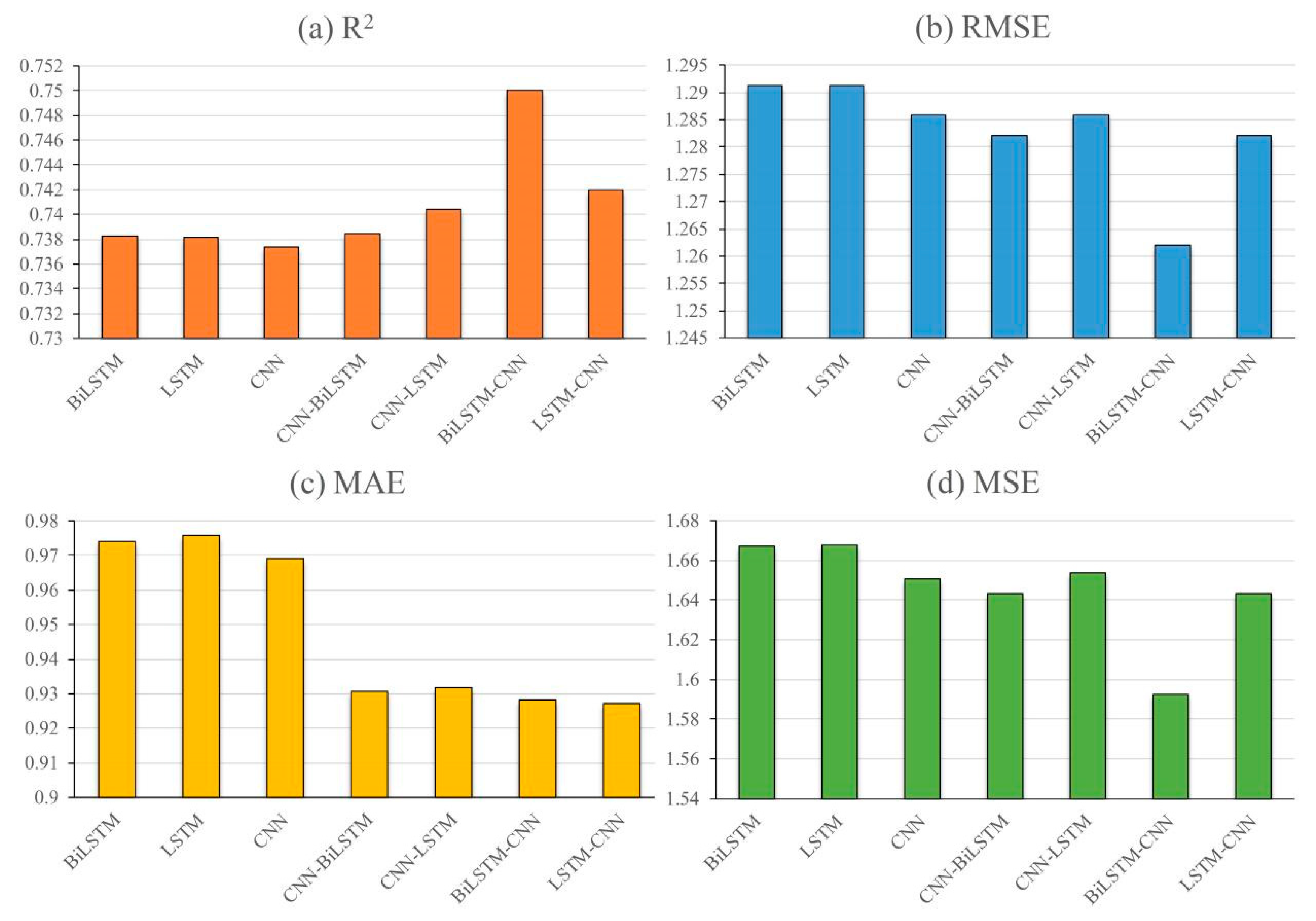
| Single Model | Hybrid Model | ||||||
|---|---|---|---|---|---|---|---|
| Bi-LSTM | LSTM | CNN | CNN-BiLSTM | CNN-LSTM | BiLSTM-CNN | LSTM-CNN | |
| RMSE: | 3.3522 | 3.5079 | 2.7343 | 2.7005 | 3.0737 | 2.5492 | 2.6307 |
| MSE: | 11.2369 | 12.3053 | 7.4766 | 7.2926 | 9.4475 | 6.4984 | 6.9204 |
| MAE: | 2.4338 | 2.7004 | 1.8983 | 1.8349 | 2.1261 | 1.7344 | 1.8296 |
| R2: | 0.9877 | 0.9865 | 0.9918 | 0.9920 | 0.9896 | 0.9929 | 0.9924 |
| Average computational time(s): | 0.2260 | 0.1274 | 0.0741 | 0.2942 | 0.1838 | 0.4752 | 0.2718 |
| Description | |
|---|---|
| 1st set comparison | CNN vs. Bi-LSTM; CNN vs. LSTM; CNN-BiLSTM vs. BiLSTM; BiLSTM-CNN vs. Bi-LSTM; CNN-LSTM vs.LSTM; LSTM-CNN vs. LSTM |
| 2nd set comparison | Bi-LSTM vs. LSTM; CNN-BiLSTM vs. CNN-LSTM; BiLSTM-CNN vs. LSTM-CNN |
| 3rd set comparison | BiLSTM-CNN vs. CNN-BiLSTM; LSTM-CNN vs. CNN-LSTM |
| CNN vs. Bi-LSTM | CNN vs. LSTM | CNN-BiLSTM vs. BiLSTM | BiLSTM-CNN vs. Bi-LSTM | CNN-LSTM vs. LSTM | LSTM-CNN vs. LSTM | |
|---|---|---|---|---|---|---|
| IR(RMSE) | 22.59% | 28.29% | 24.13% | 31.50% | 14.13% | 33.35% |
| IR(MSE) | 50.29% | 64.58% | 54.09% | 72.92% | 30.25% | 77.81% |
| IR(MAE) | 28.21% | 42.26% | 32.64% | 40.32% | 27.02% | 47.59% |
| IR(R2) | 0.42% | 0.54% | 0.44% | 0.53% | −1.04% | 0.60% |
| IR(Average computational time) | 204.90% | 71.92% | −23.19% | −52.44% | −30.66% | −53.12% |
| Bi-LSTM vs. LSTM | CNN-BiLSTM vs. CNN-LSTM | BiLSTM-CNN vs. LSTM-CNN | |
|---|---|---|---|
| IR(RMSE) | 4.65% | 13.82% | 3.20% |
| IR(MSE) | 9.51% | 29.55% | 6.49% |
| IR(MAE) | 10.95% | 15.87% | 5.49% |
| IR(R2) | 0.12% | 0.24% | 0.05% |
| IR(Average computational time) | −43.61% | −37.53% | −42.80% |
| BiLSTM-CNN vs. CNN-BiLSTM | LSTM-CNN vs. CNN-LSTM | |
|---|---|---|
| IR(RMSE) | 5.93% | 16.84% |
| IR(MSE) | 12.22% | 36.52% |
| IR(MAE) | 5.79% | 16.20% |
| IR(R2) | 0.09% | 0.28% |
| IR(Average computational time) | −38.08% | −32.38% |
Publisher’s Note: MDPI stays neutral with regard to jurisdictional claims in published maps and institutional affiliations. |
© 2020 by the authors. Licensee MDPI, Basel, Switzerland. This article is an open access article distributed under the terms and conditions of the Creative Commons Attribution (CC BY) license (http://creativecommons.org/licenses/by/4.0/).
Share and Cite
Zhen, H.; Niu, D.; Yu, M.; Wang, K.; Liang, Y.; Xu, X. A Hybrid Deep Learning Model and Comparison for Wind Power Forecasting Considering Temporal-Spatial Feature Extraction. Sustainability 2020, 12, 9490. https://0-doi-org.brum.beds.ac.uk/10.3390/su12229490
Zhen H, Niu D, Yu M, Wang K, Liang Y, Xu X. A Hybrid Deep Learning Model and Comparison for Wind Power Forecasting Considering Temporal-Spatial Feature Extraction. Sustainability. 2020; 12(22):9490. https://0-doi-org.brum.beds.ac.uk/10.3390/su12229490
Chicago/Turabian StyleZhen, Hao, Dongxiao Niu, Min Yu, Keke Wang, Yi Liang, and Xiaomin Xu. 2020. "A Hybrid Deep Learning Model and Comparison for Wind Power Forecasting Considering Temporal-Spatial Feature Extraction" Sustainability 12, no. 22: 9490. https://0-doi-org.brum.beds.ac.uk/10.3390/su12229490