Integrated Evaluation of Indoor Particulate Exposure: The VIEPI Project

Abstract

Despite the progress made in recent years, reliable modeling of indoor air quality is still far from being obtained. This requires better chemical characterization of the pollutants and airflow physics included in forecasting tools, for which field observations conducted simultaneously indoors and outdoors are essential. The project “Integrated Evaluation of Indoor Particulate Exposure” (VIEPI) aimed at evaluating indoor air quality and exposure to particulate matter (PM) of humans in workplaces. VIEPI ran from February 2016 to December 2019 and included both numerical simulations and field campaigns carried out in universities and research environments located in urban and non-urban sites in the metropolitan area of Rome (Italy). VIEPI focused on the role played by micrometeorology and indoor airflow characteristics in determining indoor PM concentration. Short- and long-term study periods captured diurnal, weekly, and seasonal variability of airflow and PM concentration. Chemical characterization of PM₁₀, including the determination of elements, ions, elemental carbon, organic carbon, and bioaerosol, was also carried out. Large differences in the composition of PM₁₀ were detected between inside and outside as well as between different periods of the day and year. Indoor PM composition was related to the presence of people, to the season, and to the ventilation regime.

1. Introduction

Environmental risks to health are defined as all the physical, chemical, biological, and work-related factors external to a person [1,2,3,4,5,6,7]. Negative effects on human health caused by exposure to atmospheric particulate matter (PM) are widely documented in the scientific literature [8,9,10,11,12,13,14], especially in the case of big cities, where the contributions of traffic and heating systems to PM sources are significant [15,16,17,18,19,20,21,22]. However, despite the fact that individuals spend about 90% of their time in indoor environments (e.g., private homes, offices, schools, transport, meeting places), most studies focusing on human exposure to PM have been carried out outdoors. Although many studies have been conducted regarding indoor air quality [23,24,25,26,27,28,29], knowledge about PM behavior in indoor environments is still not exhaustive.

PM is characterized by a great variety of chemical species and a broad spectrum of particle dimensions, the latter being a crucial parameter in the analysis of PM’s penetration into buildings and its deposition in the respiratory tree [29,30]. However, most of the scientific studies about indoor PM are limited to some classes of compounds (e.g., elements) or to some tracers of specific sources (e.g., cigarette smoke) [31,32], and only a few papers report about a complete chemical characterization of the aerosol and an in-depth evaluation of infiltration/exfiltration mechanisms [33,34].

Indoor sources of PM include cooking, domestic heating, smoking, use of electric appliances and chemical products, abrasion of textile materials, and presence of individuals [35]. In working environments, some of these sources are missing (cooking, domestic heating, smoking), and those ascribable to the presence of people become of particular importance, such as particle resuspension, clothes abrasion, and bioaerosol release (skin fragments) [36,37,38,39].

With regard to infiltration, it is quantified by the infiltration factor, which, in turn, is a function of several parameters, such as building construction characteristics (e.g., cracks, internal sources), air exchange mechanisms, outdoor meteorological conditions, and indoor air circulation [40,41,42]. The last two factors depend considerably on time, and so does the infiltration factor.

In order to assess human exposure to indoor PM, it is, therefore, necessary to quantify infiltration factor variability as well as to identify the nature, strength, and time variability of the indoor sources.

Dynamics linked to the broad variety of the spatial and time scales of some of the phenomena determining indoor pollution, e.g., PM dispersion and transformation as well as vortical structures characterizing the indoor airflow, are rather complex [43]. Such scales can be properly determined by means of a numerical–experimental approach that integrates high-frequency measurements of chemical–physical PM characteristics with computational fluid dynamics (CFD), through which it is possible to simulate both airflow and pollutant dispersion. While CFD is commonly applied outdoors, where the emission–transport–diffusion chain is generally quite easy to simulate, it is usually more complicated to apply indoors in real cases [44], mainly because of the scarcity of information regarding velocity and pressure fields needed to set the boundary conditions.

The “Integrated Evaluation of Indoor Particulate Exposure” (VIEPI) project starts from the above considerations. Its main objective is to increase knowledge on the relationships between meteorological parameters, indoor airflow, and PM concentration by means of CFD and long- and short-term field campaigns, including extensive experimental activities aimed toward chemical and biological characterization of PM as well as investigation of infiltration/exfiltration mechanisms. VIEPI was divided into the following five main activities:

• Micrometeorological and indoor airflow characterization by field experiments and CFD modeling;
• Study of the spatio-temporal variability of outdoor ultra-fine particles (UFPs) by means of a land use regression (LUR) model;
• Measurement and CFD simulation of indoor and outdoor particle number concentration at high time resolution;
• Characterization of aerobiological particles;
• Chemical and biological characterization of PM₁₀ and evaluation of the main PM₁₀ macro-sources.

In particular, VIEPI was focused on the description of the chemical and biological features of indoor suspended particles in several rooms of a building where many people gather. Great attention has been paid in the literature to school buildings because of the particular vulnerability of children to air pollution [45,46,47], as well as domestic environments [23,48,49,50]. In contrast, our attention has been paid to universities and research centers, considered as work environments that gather a very large number of students and teachers with seasonal and time slot variability.

The project took place in the Roman area from November 2016 to November 2019. Two sites were considered for the experimental campaigns: the Physics Department of the University of Rome “La Sapienza”, and one of the buildings of the Italian Workers’ Compensation Authority (INAIL) Research Center, located at Monte Porzio Catone, a small city about 10 km south of Rome. A further goal of VIEPI is to suggest recommendations on the best way to plan indoor field campaigns and to use CFD in indoor environments for air pollution assessment. Specifically, the project has the target of giving useful indications concerning (a) the optimal position of the monitoring stations (meteorological and PM) according to the geometric characteristics of the site and sampling times, (b) optimum data resolution (e.g., acquisition frequency, average period, and time slots), and (c) indications on indoor data analysis.

The objectives of this paper are (i) to give the basic rationale for the project, (ii) to describe the field campaigns, including the instrumentation and problems encountered during the experiments, (iii) to provide a description of the meteorological field that characterized the Roman area during the project, and (iv) to give a few examples of the results achieved so far, which will be further analyzed and discussed in subsequent papers of this special issue.

2. Experimental

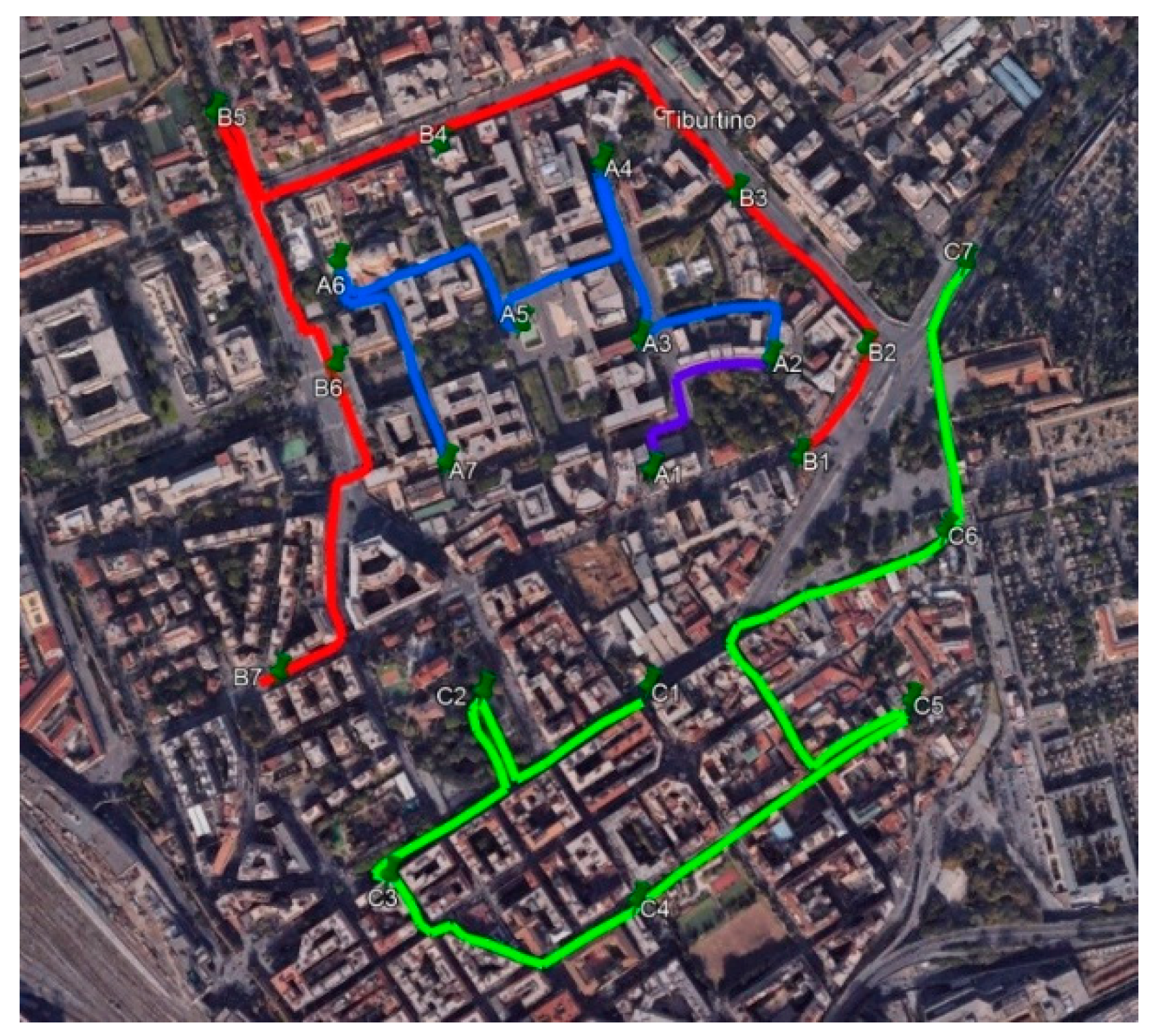
2.1. Sampling Sites and Periods

Experimental field activity within the VIEPI project took place in the greater Rome area (Italy). Two sites were considered: the Physics Department of the Sapienza University of Rome (building Enrico Fermi, Google coordinates: 41°54′06″ N; 12°30′57″ E; hereinafter: PD) and one of the buildings of the INAIL Research Center in Monte Porzio Catone (Google coordinates: 41°49′19″ N; 12°42′23″ E; hereinafter: MPC), located about 18 km southeast of the University Campus.

The PD, a five-story building covered by a terrace, was chosen because it had a number of features that made it attractive for the main goals of this project. Sapienza University is located in the center of Rome, in a morphologically heterogeneous area with buildings of different heights and shapes. Figure 1 (left picture) shows the University area and the location of the PD building (24 m high) in the southern area of the Campus. There are a number of narrow street canyons on the four sides of the building, including a main road at the south border, characterized by high traffic volumes and vehicular emission. Thermally driven sea- and land-breeze circulations typically develop in the Roman area during periods of weak synoptic forcing [51]. The mountain chains surrounding Rome contribute to the formation of anabatic (daytime) and katabatic (nighttime) winds that normally merge with the breezes for large parts of the year (see, e.g., [52,53]). These factors are conducive to the formation of a well-defined daily wind direction cycle, which deeply affects the outdoor–indoor pressure gradient in correspondence with the PD building.

Inside the building, there are a number of classrooms, laboratories, and rooms of different sizes, ranging from a wide lecture hall (about 300 seats) to small offices, which were suitable for investigating the role played by the people in determining indoor air quality and airflow circulation. The sites where the experimental campaigns of the project were carried out are reported in

Table 1. Sites of the Physics Department considered for the experimental campaigns.

Site	Abbreviation	Floor	Volume (m3)
Lecture Hall	LH	0–1	1150
Computer Room	CR	2	450
Classroom A3	A3	2–3	570
Classroom A4	A4	2–3	570
Structure of Matter Laboratory	SL	4	168
Classroom A7	A7	4–5	570
Atmospheric Physics Laboratory	AL	5	430
Terrace	T	6

; the map of the indoor sites is shown in the Supplementary Materials (Figure S1).

The lecture hall (LH), located on the ground floor, overlooks both the south and north sides of the PD building and has a double volume compared to classrooms A3, A4, and A7. Classrooms A3 and A4 and the computer room (CR) are located on the same floor. Classroom A3 faces north and looks towards the center of the University Campus. Classroom A4 faces south, over the internal courtyard, and looks towards the border of the Campus and a traffic street, about 50 m away. Both classrooms have identical volume, geometry, and capacity; they have access to an emergency staircase with an outward opening on the east side. During the winter, this door is normally closed and only occasionally opened during breaks; it remains almost systematically opened in the late spring/summer period. The CR faces east over the same courtyard as A4, and is equipped with air conditioners. Classroom A7, located on the fourth floor of the building, is identical to classroom A4. The two laboratories (SL and AL) face the internal courtyard and are also air-conditioned.

At the MPC (Figure 1, right picture), the measurements were carried out inside and outside a meeting room, which was 135 m³ in volume, and in three smaller offices of 45, 48, and 52 m³.

The VIEPI project started on February 2016 and had the duration of 33 months (until November 2019). During this period, a number of experimental studies were carried out at both the PD and MPC sites in order to build a robust database supporting the activities.

Sampling periods within Activity 1 (micrometeorological and indoor airflow characterization by field experiments and CFD modeling) covered the whole duration of the project, with preliminary field studies carried out at the MPC during 2016 and many intensive observation periods run at the PD during the following two years (in the AL during the winter 2017–2018 and in the CR from March 2018 to June 2019).

Experimental campaigns within Activity 2 (spatio-temporal variability of outdoor UFPs) were carried out for seven consecutive days in November 2017 and in June 2018 in a 1 km × 1 km area surrounding the University Campus and centered on the PD (21 points in the study domain).

Field observations within Activity 3 (indoor and outdoor particle number concentration) consisted of four intensive periods during both winter and summer in order to capture different weather conditions and conditions of use of indoor environments typical of the cold and warm seasons (November–December 2017, June 2018, November–December 2018, June 2019). They were carried out in LH, CR, A3, A4, and A7.

Activity 4 (aerobiological particles) was carried out at the MPC with some preliminary monitoring periods during the period June 2016–July 2017 and, continuously, at the PD from November 2017 to November 2018.

In the framework of Activity 5 (chemical and biological characterization of PM₁₀), two types of field studies were conducted. The first one (short-term intensive campaigns) was carried out during three periods: November–December 2017, June 2018, and November–December, 2018. PM₁₀ samples were simultaneously collected at five indoor sites (LH, CR, A4, SL, and A7) and outdoors (on the ground floor). The sampling schedule was designed to obtain five samples a week: two during lesson times (from 09:00 to 18:00 local standard time, LST), two during the evening/night, when the rooms were empty (from 18:00 to 09:00 LST of the following day), and one during the weekend. The second type of study (long-term campaign) was continuously carried out from November 2017 to October 2018, with 12 sampling periods of the duration of one month. Indoor sampling sites were in LH, CR, A3, A4, SL, and A7. Each sampling was simultaneously performed indoors and outdoors, out of the window and at the same height from the ground. Measurements of both PM₁₀ and PM_2.5 were carried out. Two additional outdoor sampling points were set on the roof of the PD building and the roof of another building that was about 50 m away.

2.2. Equipment

2.2.1. Activity 1: Micrometeorological and Indoor Airflow Characterization by Field Experiments and CFD Modeling

Wind velocity and air temperature were measured both inside and outside the PD building. In particular, one sonic anemometer/thermometer (Gill Instruments Limited, Lymington, UK, acquisition frequency of 32 Hz) was mounted on a 3.5 m mast located on the terrace (i.e., z = 1.14H, where z is the height), while two sonic anemometers (Gill Instruments Limited, 4 Hz) were mounted on a metallic brace 80 cm outside one of the windows on the second and fifth floor, in correspondence with the CR and AR (Figure 2). Two sensors of differential pressure (Delta Ohm, Caselle di Salvazzano, Italy, 1 Hz) were installed on the same windows to collect outdoor-indoor pressure differences. The pressure differences between the two rooms and the corresponding hallways were measured by means of two other differential pressure sensors. Indoor measurements of velocity and temperature were collected in the CR and AL by means of two sonic thermometer/anemometers (Gill Instruments Limited, 20 Hz).

In addition, a triaxial monostatic Doppler SODAR (Sonic Detection and Ranging) system (APM-301) located on the terrace permitted investigations of the three components of the wind velocity up to an altitude of about 200 m with approximately 7.5 m vertical resolution (see [54,55] for details). The SODAR belongs to the BAQUNIN (Boundary-layer Air Quality analysis Using a Network of Instruments, https://www.baqunin.eu/) super-site urban location. BAQUNIN also hosts an elastic LIDAR (Light Detection and Ranging) through which it is possible to retrieve vertical aerosol profiles for a large part of the troposphere (spatial and temporal resolution: 7.5 m and 10 s, respectively) and the planetary boundary layer (PBL) height [56,57].

The CFD software ANSYS Fluent 18.2 [58] was employed to simulate airflow and PM dispersion for several case studies.

2.2.2. Activity 2: Spatio-Temporal Variability of Outdoor UFPs

Spatio-temporal generalized additive models (GAMs) were developed to describe the spatio-temporal variability of the ultrafine particles (UFPs) at the microscale level and to identify the main descriptors of such variability. The total monitored particle number concentration (PNC, as a proxy of the UFPs) data were used as response variable. The 21 points of the study domain were chosen so as to obtain measurements representative of the maximum spatial gradient of detectable concentration in the area, assuming the road traffic to be the main source of UFPs in the urban context.

The PNC measurements were made using portable condensation particle counters (3007 TSI) for one week (10 min for each site, three times a day), following paths characterizing the area of study (Figure 3): route A (blue) University Campus; route B (red) external perimeter of the University Campus; route C (green): San Lorenzo district.

Due to the large number of measurement sites along with the limited number of available devices (four), a rounding measurement strategy was adopted, sharing devices among monitoring sites. Geographic information system (GIS) analyses were conducted to derive the spatial variables at each monitoring site. The set of spatial predictors included the traffic intensity, distance to the nearest local and major roads and their various combinations, total length of major and local roads, land cover variables (high-density residential land, low-density residential land, commercial and public urban areas, urban green), and population density, all calculated in several small circular buffers.

To represent the height and the continuity of street canyons, four variables for buildings and/or street configurations were designed.

The temporal variables acquired for use as potential predictors were meteorological parameters (wind speed and direction, air temperature, relative humidity, pressure, precipitation, global solar radiation) and micrometeorological parameters (standard deviation of the horizontal and vertical wind speed module, turbulent kinetic energy, z/L stability parameter (L is the Obukhov length), and atmospheric stability classes) (Pasquill–Gifford). Moreover, only during the summer period, the PBL height was calculated by vertical aerosol profiles measured using LIDAR combined with SODAR data.

2.2.3. Activity 3: Indoor and Outdoor Particle Number Concentration

Total particle number concentration (TPNC) was simultaneously measured indoors and outdoors by using co-located condensation particle counters (CPC3007, TSI Inc., Shoreview, MN, USA, min detectable particle (D50): 10 nm, time resolution: 1 s). In the CR and LH, at the same time as the aforementioned measurements, size-resolved PNC measurements were carried out to study the temporal variability of the dimensional distribution in number of particles from 10 nm to 10 µm using a scanning mobility particle sizer and optical particle sizer (SMPS 3910, Fast Mobility Particle Sizes (FMPS) mod. 3091, OPS 3330 TSI Inc., Shoreview, MN, USA). Moreover, measurements of the average and cumulative lung-deposited surface area (LDSA, in µm²/cm³) of particles from 10 nm to 1 µm, corresponding to the tracheobronchial or alveolar pulmonary fractions, were carried out by using a nanoparticle surface area monitor (NSAM mod. 3550, TSI Inc., Shoreview, MN, USA; 1 s time resolution). Additional measurements also included: PNC (#/cm³), average diameter (nm), and LDSA (µm²/cm³) with a time resolution of 1 s by a mini diffusion size classifier (DM-UF5, mod. TESTO), size distribution (dN/dLogDp) and TPNC (#/cm³) in the size range of 6 nm–10 µm, with 1 s time resolution using an electric low-pressure impactor (ELPI+, mod. Dekati), and polycyclic aromatic hydrocarbons (PAHs) surface-adsorbed on carbon aerosol in the size range 10 nm–1.5 µm using a photoelectric aerosol sensor (PAS2000, EcoChem Analytics, League City, TX, USA).

2.2.4. Activity 4: Aerobiological Particles

Aerobiological particles 10–100 µm in diameter were collected in compliance with the UNI 11108/2004 [59] and following UNI CEN/TS 16868:2015 [60] using a seven-day volumetric Hirst type sampler (Lanzoni VPPS^® 2000, Bologna, Italy). The sampling method is based on the impact of particles on a surface consisting of a transparent plastic Melinex^® (TEKRA LLC., New Berlin, WI, USA) tape coated with a 2% silicon solution. The tape moves with a speed of 2 mm per hour on a cylindrical drum that makes a complete round in a week. Air sucking is provided by a vacuum pump operating at the flowrate of 10 L/min, matching the human breathing rate. The system is tailed directionally, allowing it to be continually oriented against the wind. The outdoor sampler is placed at a standard height of about 15–20 m from the ground; in these conditions, it is able to monitor an area of about 15 km radius. The Hirst sampler is designed to detect the atmospheric concentration of biocontaminants, such as pollen and fungal spores, using morphological recognition. Following a weekly air monitoring, the stripes are cut into daily segments, placed on single glass slides, stained using glycerine jelly with fuchsine, and then observed with an optical microscope (magnification: 40×) for the count and characterization of pollen and fungal spores [61].

2.2.5. Activity 5: Chemical and Biological Characterization of PM₁₀

Short-Term Intensive Campaigns

In each room and at the outdoor site, we set three PM₁₀ samplers. Given the necessity to avoid any inconvenience to teaching and research, we used very quiet samplers (<35 dB) specifically designed for use in indoor environments (Silent Sequential Sampler, FAI Instruments, Fonte Nuova, Rome, Italy) operating at the flow rate of 10 L min⁻¹. Each sampler was equipped with a sequential system able to run four sampling lines without attendance. Outdoors, each sampling line was provided with a cap to protect the inlet from wind and rain.

In all cases, PM samplings were simultaneously carried out on Teflon (TEFLO, 47 mm, 2.0 micron pore size, PALL Italia, Buccinasco, Italy), quartz (TISSUQUARTZ 2500QAT, 47 mm, PALL Italia, Buccinasco, Italy), and polycarbonate filters (47 mm, 0.8 μm pore size, MILLIPORE, Merk Life Science, Milano, Italy).

Teflon filters were used for the determination of PM₁₀ mass concentration by gravimetry, using an automated microbalance (mod. ME5, 1 μg sensitivity; Sartorius AG, Goettingen, Germany), after conditioning at 50% Relative Humidity and 20 °C for 48 h. Then they were analyzed using energy-dispersion X-ray fluorescence (X-Lab 2000 and XEPOS, Spectro Analytical Instruments, Kleve, Germany) for the contents of Si, Al, Fe, Na, K, Mg, Ca, and minor elements. Then, the filters were extracted in deionized water and analyzed for ions (chloride, nitrate, sulfate, sodium, potassium, ammonium, magnesium, and calcium) by ion chromatography (ICS1000, Dionex Co., Sunnyvale, CA, USA). Finally, the soluble and residual fractions of 23 elements were analyzed by sequential extraction and inductively coupled plasma mass spectrometry (ICP-MS, Bruker 820 MS, Billerica, MA, USA). This overall procedure, which allows a high number of analytical determinations on the same filter, is described in detail in [23,62,63].

The determination of the organic and elemental carbon was carried out on quartz filters using thermo-optical analysis (OCEC Carbon Aerosol Analyzer, Sunset Laboratory, Tigard, OR, USA) and the NIOSH-QUARTZ thermal protocol. Samples collected in the A4, CR, and outdoors were also analyzed for the content of eight carcinogenic and mutagenic congeners of polycyclic aromatic hydrocarbons (PAHs) included in the Environmental Protection Agency priority list: benzo(a)anthracene (BaA), benzo(b)fluoranthene, benzo(j)fluoranthene, benzo(k)fluoranthene (BbjkF), benzo(a)pyrene (BaP), indeno(1,2,3-cd)pyrene (IP), dibenzo(a,h)anthracene (DBahA), and benzo(g,h,i)perylene (BPE). They were extracted from the quartz membrane using sonication with dichloromethane/acetone sequence and concentrated. The obtained low-volume samples were analyzed by using a gas chromatograph (6890N Agilent Technologies, Santa Clara, CA, USA) equipped with a mass-selective detector (5973N Agilent Technologies). The validation of the analytical method was carried out according to the guidelines given by the EURACHEM (1998) by using the certified urban dust (SRM 1649a), which was purchased from the National Institute of Standards and Technology (NIST) (Gaithersburg, MD, USA).

Polycarbonate filters were used for the evaluation of the bio-aerosol content by a method involving propidium-iodide staining, optical microscopy observation, image processing, and calculation of the mass concentration. Details of the procedure are described in [64].

Outdoors, we also added a dual-channel beta attenuation monitor (and sampler) operating at the flow rate of 2.3 m³/h, compliant with the requirements of the regulations about outdoor PM measurement (SWAM 5a Dual Channel Monitor, FAI Instruments, Fonte Nuova, Rome, Italy). The monitor was equipped with Teflon and quartz filters and was operated on a 24 h basis. The samples were analyzed for the same species and by following the same analytical methods described above.

Long-Term Campaign

In this case, we used very low flow-rate samplers (Smart Sampler, FAI Instruments—Roma, Italy) operating at the flow rate of 0.5 L/min. Four samplers were placed in each indoor and outdoor site. Three of them were devoted to PM₁₀ measurement and equipped with Teflon, quartz, and polycarbonate filters, respectively. The fourth one was fitted with a Teflon filter and a PM_2.5 impactor to obtain more information about the size distribution of PM components and the dependence of infiltration on particle size.

2.2.6. Quality Control

The particle counters and particle sizers were calibrated in the factory before each one of the two sampling campaigns using monodisperse artificial aerosol. Moreover, in the cases of both particle counters and meteorological instruments, during the project, we adopted a Quality Control procedure consisting of devoting one day before the start of each experimental campaign to the inter-calibration of the instruments and comparison of the obtained experimental results.

The flow rate of the indoor PM₁₀ samplers was checked once a week by using an external mass flow meter. The dual-channel monitor used for outdoor PM₁₀ sampling was subjected to an internal span check and leak test procedure that was run daily before the start of each sampling period.

The overall analytical method applied to the chemical characterization of PM₁₀ has been widely validated in previous studies. A detailed discussion of the applied Quality Assurance/Quality Control procedure is reported in [62].

3. Results and Discussion

3.1. Activity 1: Main Characteristics of the Outdoor Airflow

The near-surface wind field observed during VIEPI activities was in line with what was found in previous studies concerning meteorological analysis conducted in the Roman urban area (e.g., [65,66]). During the spring, summer, and autumn, the wind was mostly oriented along the southwest–northeast axis as a result of the diurnal wind cycle caused by the sea–land-breeze regime characterizing the region (see Figure S2 in the Supplementary Materials).

Figure 4 shows the scatter plot of the wind direction as a function of the time of day in which the measurement took place during April 2018 by the SODAR and by the three anemometers installed outside the PD building. The diurnal behavior of the wind direction shows a marked day-to-night variation both above the building (z = 1.4H and z = 1.14H) and within the canyon (z = 0.8H), even though in the latter case, the wind speed is considerably lower. At all three locations, it is possible to recognize two distinct clusters in the wind direction pattern. One is concentrated between south and west from 12:00 to 20:00 LST, and the second between north and east from 20:00 LST to 12:00 LST. Note that the nocturnal regime at z = 0.8H appears more concentrated in the north–northeast sector. This is reasonable in that the façade where the sonic anemometers are installed is oriented nearly 20° from north (see Figure 1 and Figure 2).

Even more pronounced effects of the façade’s orientation on the wind direction are observed on the second floor (z = 0.4H), where two much narrower clusters (southwest and north–northwest), are present irrespective of the time of day. The wind, therefore, is parallel to the façade regardless of the wind direction above the terrace. However, it is worthwhile to remember that wind speed and direction over building walls change considerably with height and approaching wind direction, even for building arrangements much simpler than the one considered in the present case (e.g., [67,68]).

Additional information on the flow field with respect to the PD building was also inferred from CFD. This tool has become attractive at the microscale because of its ability to simulate airflows for real building arrangements, complex scenarios, and different research fields (e.g., [69,70,71]). ANSYS Fluent 18.2 was used, adopting the standard k-ε turbulence closure based on the 3D Reynolds-averaged Navier–Stokes (RANS) equations. The computational domain and grid (see Figure S3 in the Supplementary Materials) were set according to the guidelines [72,73].

The numerical simulation refers to 16:00 LST on 21 April 2018. The idea behind this is that in the area of interest, in case of clear skies and weak synoptic forcing, the wind direction in the afternoon is fairly constant for several hours due to the breeze regime (nearly from southwest). This simplifies the analysis and facilitates the comparison between numerical and experimental results. A logarithmic wind-speed profile based on data taken from the meteorological station located at G.B. Pastine Airport in Ciampino, about 10 km southeast of Rome, was imposed at the inlet.

Figure 5 (left panel) shows the contour map of the wind speed simulated on the horizontal plane at z = 0.4H (second floor). The flow pattern shows high complexity and inhomogeneities. The wind comes from southwest and is deflected by the features located upstream of the PD building. The velocity is higher in the streets corresponding with the west and south façades, whereas it is considerably lower (about 0.7 ms⁻¹) in the canyon on the east side (i.e., between the PD building and the adjacent Chemistry Department). The corresponding pressure field (Figure 5, right panel) shows that between the PD façades, the maximum differential pressure is about 0.75 Pa. This value is large enough to generate an indoor airflow from the west to the east façade. It is worthwhile to mention that the indoor/outdoor differential pressure measured at z = 0.4H is nearly approximately 0.7 Pa. However, note that the pressure distribution over building walls is expected to change considerably with the approaching wind direction (e.g., [74]). Consequently, the use of wind-speed data measured on the terrace is often useless for the purpose of calculating the pressure acting on the walls of buildings.

The vector field of the wind speed over the vertical plane perpendicular to the east façade (passing through the point where the sonic anemometer on the second floor is located) shows the well-defined vortical structure typically observed in canyon flows (e.g., [75,76]), i.e., a current descending in the portion close to the Chemistry Department and ascending near PD (Figure S4 in the Supplementary Materials). That kind of structure is usually responsible for the transport and dispersion of pollutants emitted at street level, which can thus reach the highest floors of the building [77].

The agreement between modeled and observed horizontal velocity is rather good above the building (z = 1.4H and z = 1.14H) and reasonable at z = 0.4H, whereas the error is larger at z = 0.8H (Table S1 in the Supplementary Materials). Therefore, the model does not reproduce the turbulence structures within the canyon very well, even if the mesh has been refined near the walls. We should also consider the fact that the shape, size, and direction of rotation of vortical structures within canyons depend considerably on the angle between the approaching flow and canyon axis (e.g., [78,79,80]). Moreover, non-stationarities intrinsic of the real approaching flow make the agreement between observation and simulation very challenging within the canyon.

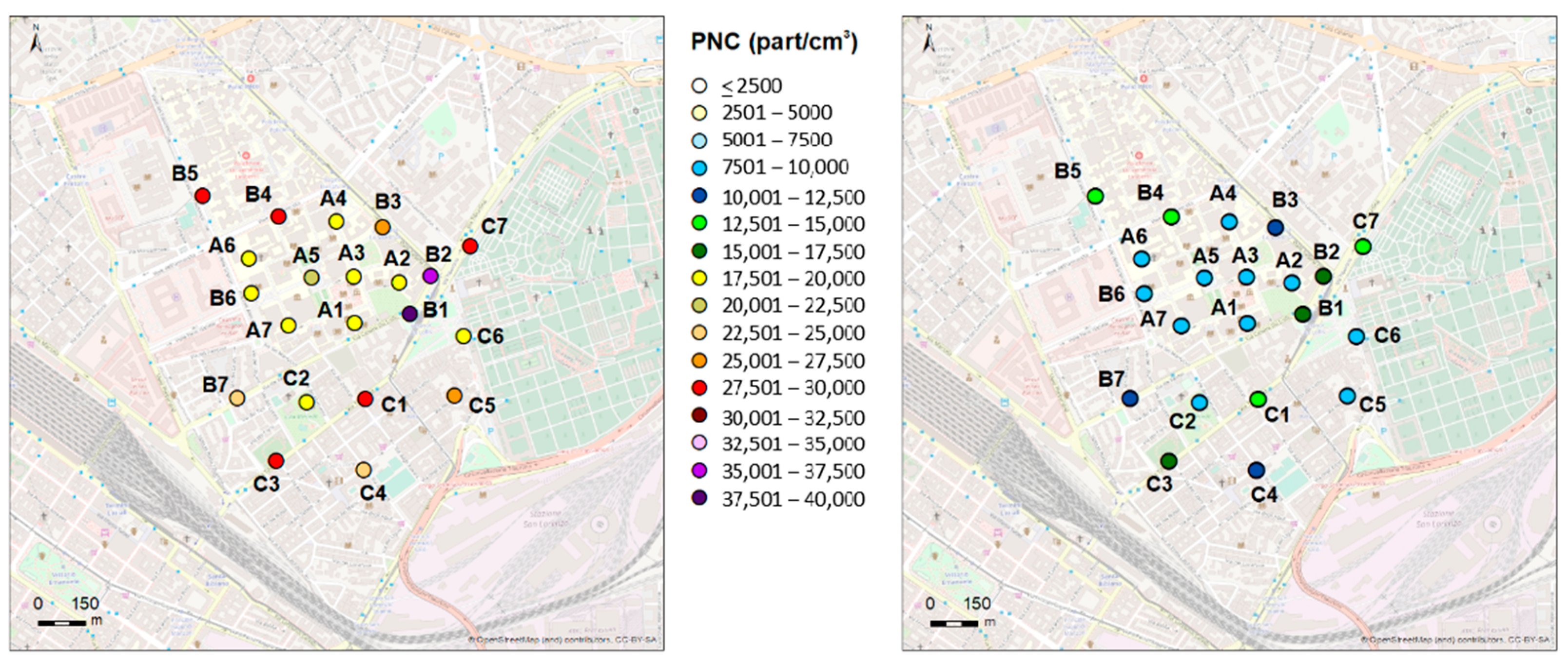
3.2. Activity 2: Spatio-Temporal Variability of Outdoor UFPs

The PNC was the response variable used to assess the spatio-temporal variability of outdoor UFPs using GAM models. Here, we show the results of the monitoring campaigns, while the calculation of the main parameters for urban morphology description and the development and validation of a land use regression (LUR) model for PNC estimation will be reported elsewhere.

The chosen sites were characterized with respect to the main local source (i.e., road traffic) using both distance from the nearest road and traffic flow therein. They potentially allowed us to catch a large portion of microscale spatial variability, since the median of the ratios of traffic flow by distance ranged between 0.2 and 280 vehicle h⁻¹ m⁻¹.

Figure 6 shows average PNC values at the measurement points selected in the study area. The PNC recorded in the university area (A1–A6, cars allowed for restricted personnel only) were significantly lower than those observed in the two external routes (PNC_A1–A6 = 13,724 part/cm³ and PNC_A1–A6 = 19,645 part/cm³, respectively). The points close to roads with high traffic flows were points B1, B2, B3, B4, B5 (quadrilateral outside the university), C1, C3, and C7 (on Via Tiburtina, the main busy road). The average concentrations in points B6, C2, and C6, relatively far from the busiest roads, are comparable in both seasons with those of the sites within the University Campus (PNC_B6-C1-C6 = 12,959 part/cm³ and PNC_A1-A6 = 13,724 part/cm³, respectively).

While several studies attempted to assess the spatial variability of PNC and other pollutants at the local/urban scale through statistical modeling based on dense monitoring in a wide spatial domain (e.g., [81,82,83,84]), only a few studies have addressed whether the spatial variation of particle number concentration (PNC) within a microscale environment can have an effect on exposure estimation results (e.g., [85]).

Vehicle emissions clearly increase background particle concentrations. In particular, UFPs are characterized by a sharp spatial decline from the emission sources, since they are removed through coagulation processes. Thus, it is expected that nearby traffic load and distance from major roads could be relevant explanatory variables for UFPs’ spatial pattern, together with land use variables (e.g., population density, urban green).

The monitoring results allow us to confirm the large spatial variability of PNC still existing on the microscale (here, 1 km × 1 km), likely leading to significant differences in exposure pattern. This should be taken into account when assessment of indoor to outdoor ratios is carried out using a single or a few fixed outdoor sites in the study area. Moreover, the spatial variability needs to be further investigated, since, other than the relative distance to traffic, the urban morphology can be a relevant factor explaining such variability.

Winter PNC values (PNC_winter = 24,170 part/cm³) were about twice the summer ones (PNC_summer = 11,173 part/cm³), as expected based on previous studies carried out in Rome (e.g., [86,87]).

The excellent linear correlation between the average PNC recorded at each site during winter vs. PNC during summer (R² = 0.86) accounts for the fact that the spatial gradient in the domain under examination is comparable in the two seasons. Moreover, a clear daily pattern was found: maxima were found during winter rush hours (early morning and mid/late afternoon) that are often coincident with the lowest mixing height observed during the daylight hours.

During winter, the morning and evening PNC peaks at rush hours can be considered the result of the motor vehicle emissions combined with a lower diurnal mixing layer height and lower ambient temperature, which favors nucleation mechanisms, at least for particles with dimensions up to some tenths of a nanometer (e.g., [88]).

The morning peak still present in summer months might be related predominantly to particles directly emitted by road traffic. The more favorable diurnal conditions for atmospheric dispersion during the warm season lead to lower absolute values of PNC.

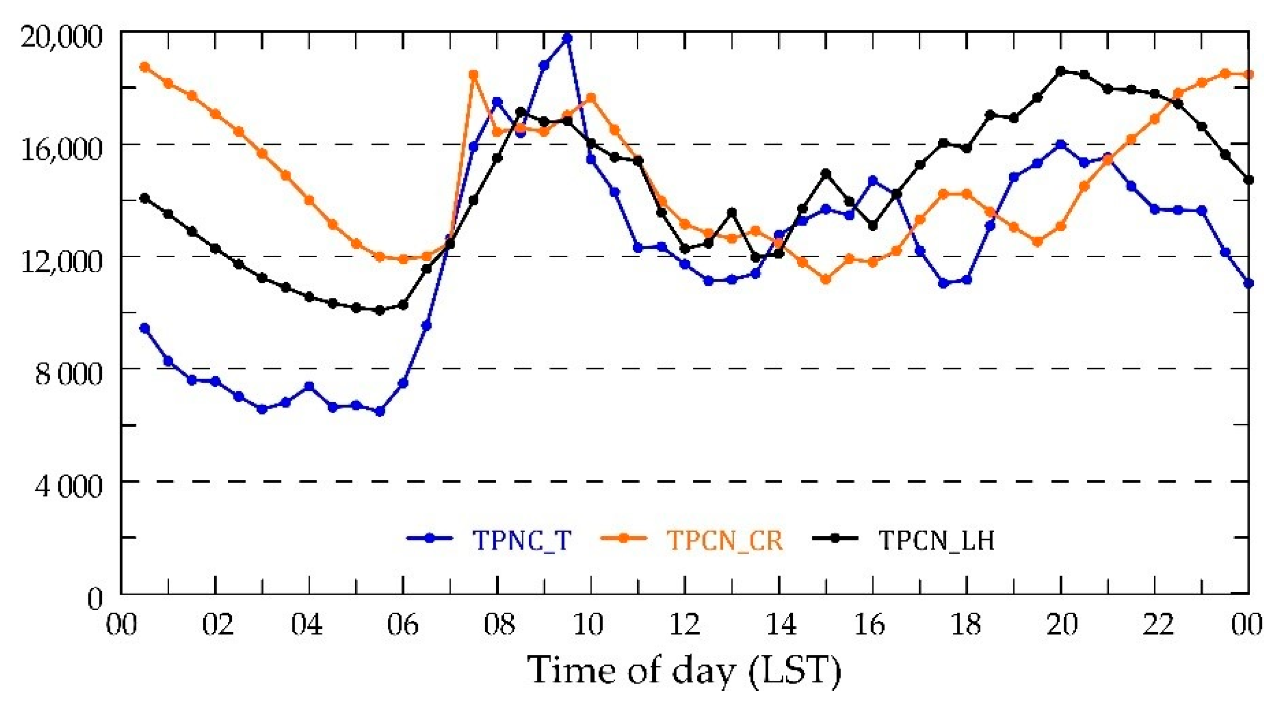
3.3. Activity 3: Indoor and Outdoor Particle Number Concentration

To assess the possible observable differences between classrooms located on the same floor, but with different orientation of the windows with respect to the outside, three classrooms were selected: A3, A4, and CR, all located on floor 2 (Supplementary Materials, Figure S1). To evaluate the possible observable differences between classrooms located at different heights from the ground, two classrooms were selected: LH and A7. The measurement campaigns were carried out in different seasonal periods in order to capture different weather conditions and conditions of use of indoor environments typical of cold and warm seasons.

Descriptive statistics (

Table 2. PNC (part/cm³) of classrooms located on the same floor (floor 2); winter and summer campaign descriptive statistics.

		A3	Outdoor A	CR	A4	Outdoor B
Summer 2018	Mean	13,308	12,418	N.A.	13,916	12,802
	Median	11,315	11,482	N.A.	12,555	11,631
	Min	3722	3188	N.A.	4409	2447
	Max	40,008	95,178	N.A.	41,665	45,241
	SD	6666	6363	N.A.	6419	6192
Winter 2018	Mean	10,781	15,328	11,198	12,472	16,296
	Median	10,378	12,943	9454	11,683	14,075
	Min	2552	5265	5822	3622	5670
	Max	49,505	50,832	38,661	35,594	46,898
	SD	4283	7070	4609	4292	7492

and

Table 3. PNC (part/cm³) of classrooms located at different heights from the street level (ground floor and floors 2 and 4); winter and summer campaign descriptive statistics.

		LH Ground Floor	CR Floor 2	A7 Floor 4	Outdoor A	Outdoor C
Summer 2018	Mean	9714	7402	N.A.	10,747	9907
	Median	9591	7264	N.A.	9858	9413
	Min	4523	3987	N.A.	3291	2563
	Max	19,383	11,509	N.A.	64,947	45,179
	SD	2903	1780	N.A.	4542	4443
Summer 2019	Mean	6659	N.A.	11,776	12,066	12,005
	Median	6235	N.A.	10,497	10,601	10,659
	Min	4755	N.A.	4661	5309	5746
	Max	13,080	N.A.	31,576	45,077	44,396
	SD	1544	N.A.	5284	4727	4651
Winter 2018	Mean	10,882	12,049	14,109	21,833	16,641
	Median	9688	11,587	11,818	21,231	16,369
	Min	6746	5011	6411	5785	5229
	Max	20,546	28,037	93,918	111,760	68,662
	SD	3099	3712	6680	8864	6049

) are reported for both the horizontal and vertical gradient assessments.

A clear seasonal pattern was found linked both to different ways of classroom use and meteorological conditions. In June, classrooms were occupied rather discontinuously, with alternating periods of zero or very limited occupation and periods of greater crowding. The prevailing ventilation conditions were those typical of the summer period (natural ventilation with open doors and windows; air conditioners turned on in LH and CR). During winter, the scenario was radically different: systematic occupation of the classrooms with a succession of teaching activities without interruption from 08:00 to 18:00 LST on most days. However, since particularly cold days did not occur, it was often observed that the upper doors directly opening to the outside were open.

Concerning indoor measurements, the horizontal gradient showed very similar PNC values between the two sides, with the same modulation in summer and slightly higher concentrations in the classroom on the street side. As regards the indoor vertical gradient, the PNC values were higher in the classroom on the fourth floor than in the LH on the ground floor, but this difference is influenced by the different geometries and uses of the considered classrooms rather than by the altitude relative to the ground.

As for external measurements, in the comparison between the two measurement points on the north and south sides of the same floor, the PNC levels were very similar and with the same modulation, with slightly higher concentrations on the road side. The comparison between the outdoor measurements on the ground floor and on the fourth floor shows higher PNC values at the lowest level, with excellent correlation between the two time series.

The preliminary results related to the autumn–winter campaign have been reported in Boccuni et al. [89].

Data of PNC and particle size distribution (PSD) measured by FMPS for airborne UFPs in the size range 5.6–560 nm were collected during a working week at three different heights. Nighttime measurements were also performed to include non-working activities.

In general, the average daily trends (Figure 7) suggested that multiple factors influenced UFPs’ PNC levels, probably related to both outdoor and indoor contributions. In particular, at the beginning of the day, in the transition hours (from 05:00 to 07:00 LST), we noted an increase in outdoor UFPs’ PNC, probably due to the starting of anthropic activities; the indoor values reflect the same structure with a certain delay time. During the daylight hours (from 07:00 to 16:00 LST), the outside component outnumbers the influences from other internal sources of PNC. In the transition from daylight hours to the night (from 16:00to 18:00 LST), a general increase of PNC in indoor sampling points was mainly recognized. The outdoor average daily trends of UFPs’ PNC confirm the daily profiles of population mobility indicators already proposed by [90] for the city of Rome in their study on urban population mobility using mobile phone traffic data.

The study in the spring on 19–21 June 2018 confirmed that FMPS and DM-UF5 at z/H = 1.1 are linearly correlated. They are also sensitive in monitoring different particle-size distributions. The best correlation between the two instruments was achieved at nighttime, when a steady state can be assumed for the contributions of meteorological conditions and sources, which are suitable for proper measurement either by FMPS or DM (Figure S5 in the Supplementary Materials). During this period, the daily PNC vertical gradient was positive, equal to about 170 (#/cm³)/m.

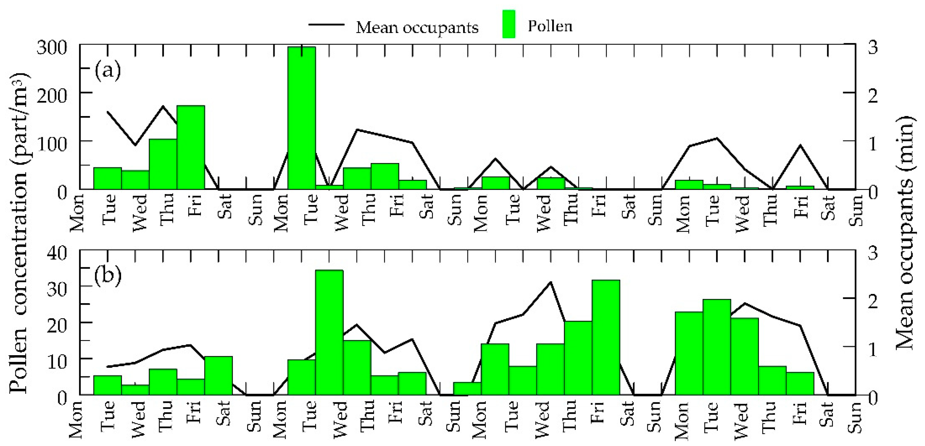
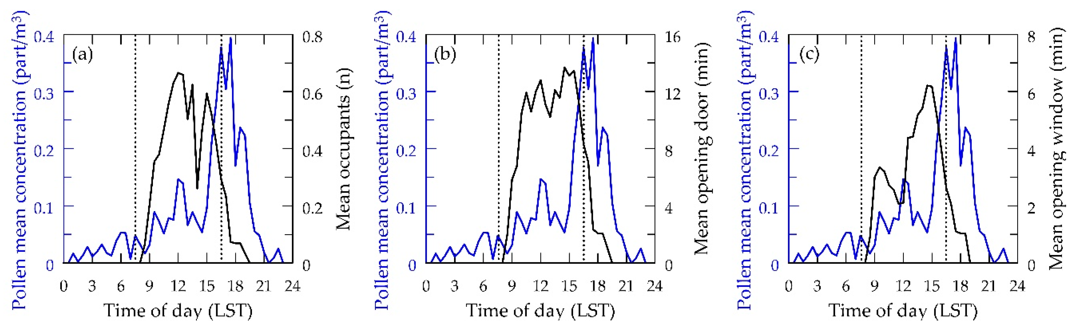
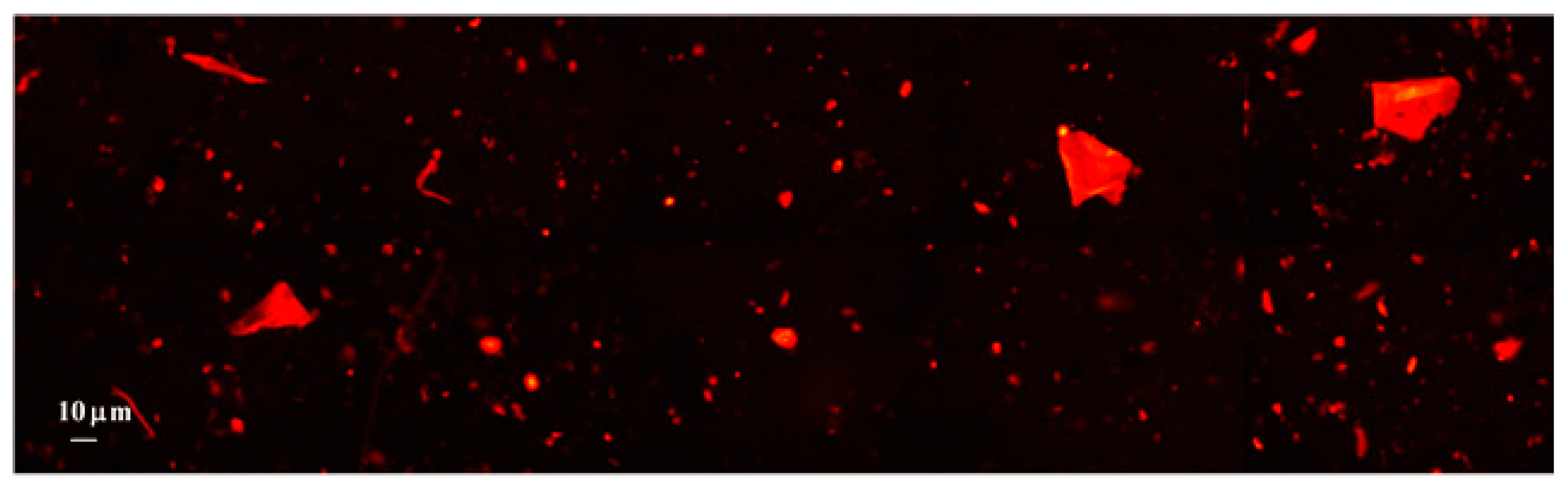
3.4. Activity 4: Aerobiological Particles

The results of the preliminary campaigns seem to indicate an increase of aerobiological particle concentrations during working hours in relation to workers’ presence and behavior. Workers interact continuously with the indoor environment to realize their thermal and physiological comfort (window and door opening/closing or turning off ventilation), as shown in

Table 4. Example of a spreadsheet (based on [91]) developed to detect workers’ presence, behavior, and microclimatic variables in indoor workplaces of the Research Center in Monte Porzio Catone (MPC) (O: Open; C: Closed).

Time of Day (LST)	Door (min)	Window (min)	Fan (min)	Occupants (n)	Tair (°C)	Relative Humidity (%)	Wind Speed (ms−1)
07:30–08:00	O/C	C/O	Off/On	1	26.5	41.7	0.1
…	C/O	C/O	On/Off	5	23	59	0.23
…	C/O	O/C	On/Off	3	28.1	67	0.13
19:30–20:00	O/C	C/O	Off/On	2	27	44	0.05

.

The preliminary results were obtained through aerobiological monitoring in the MPC, that is, an area characterized by the Holm oak range, which consists of mixed oak woods with Quercus ilex and deciduous trees, with prevalence of cultivated species such as Olea europaea and Vitis vinifera. The Research Center of the MPC is surrounded by herbaceous plants, hedges, coniferous trees, olive groves, and vineyards.

During the non-working days (from Saturday to Sunday) or in absence of occupants, the biocontaminant values decreased. Figure 8 shows pollen trends in relation to the occupants observed in the summer campaigns. By looking these trends, the relationship between occupants and biocontaminants is mostly evident with respect to the non-working days. These results suggest that the presence of the occupants is an important factor contributing to the indoor concentrations of biocontaminants, such as pollen.

Occupants’ presence and behavior may affect diffusion and concentration of aerobiological particles as well as microclimatic parameters, which, in turn, may themselves affect pollens and fungal spores. In fact, during the summer, the microclimatic monitoring showed that the mean air temperature is higher (25.9 °C), while in the non-working days, it is lower (24.5 °C); mean relative humidity is higher (50.1%) in the non-working days with respect to the working days (49.7%). Our data do not seem to indicate a relationship between the aerobiological particles and the T_air and relative humidity, while the W_S trend decreases in non-working days, as do the pollen and fungal spores’ trends (Figure S6 in the Supplementary Materials).

It is worth noting that occupants’ actions, such as opening of doors and windows, affect biocontaminant values during working and non-working periods, as shown in Figure 9 for pollen.

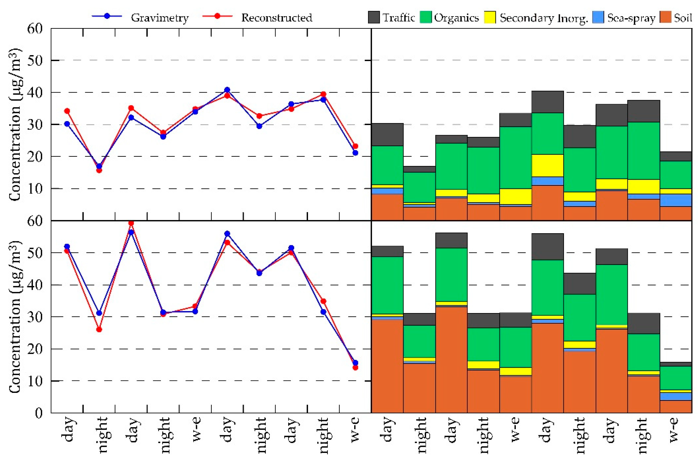
3.5. Activity 5: Chemical and Biological Characterization of PM₁₀

In this paragraph, we discuss the chemical and biological characterization of PM₁₀ obtained during the short-term intensive campaign carried out during the winter of 2018 (for the description of the campaign schedule, see Section 2.1, activity 5).

The first step in the evaluation of the results was a check of the mass closure, that is, the correspondence between the mass concentration determined by gravimetry and the sum of the individual chemical determinations (reconstructed mass) obtained by applying appropriate conversion factors for non-measured elements (typically H or O). Very satisfactory results were obtained, with the sum of the chemical measurements accounting for 93–115% of the gravimetric mass, and a Pearson’s coefficient of the scatter plot (R²) in the range of 0.91–0.97 (winter campaign 2018). The results of the chemical characterization were then elaborated to obtain a robust evaluation of the strength of the primary sources of PM: soil, sea-spray, secondary inorganics (ammonium nitrate and ammonium sulphate), organics, and traffic. The algorithms used for calculating the macro-sources are widely described in [62,63,92] and are briefly reported in Appendix A.

Figure 10 shows the mass closure for PM₁₀ samples collected outdoors and in one of the two classrooms located on the third or fourth floor during the period 26 November–9 December 2018 (left panels). In the same figure, we report the day-by-day variation in the strength of the PM₁₀ macro-sources at the same sites (right panels). We chose classroom A4 because it was the more crowded one during classes and it showed the widest day–night variations. The mass closure was very satisfactory, as the reconstructed mass constituted 97% ± 7% of the gravimetric mass outdoors and 102% ± 8% indoors. The data show that indoor concentrations widely exceeded outdoor values during the daytime, while they were closer to each other during the other periods. On average, the indoor increase in concentration recorded during the daytime samplings was as high as 16.5 μg/m³, while it was only 5.1 μg/m³ during the night periods. During the weekends, outdoor values exceeded indoor concentrations by 5.3 μg/m³.

The study of the macro-sources shows that the indoor increase in the mass concentration of PM₁₀ during weekdays was mainly due to an increase in soil components. This contribution was mostly due to the presence and movements of the students and to the use of chalk; it was found to be related to both the occupancy rate in the classroom and the duration of the lessons. Soil components are brought inside attached to the shoes and clothes of the students; moreover, particles already deposited on the floor and other surfaces are re-suspended when people walk and move. On average, the indoor increase in the concentration of this component recorded during daytime was 20.3 μg/m³. The indoor-to-outdoor ratio (I/O) ranged between 4.8—recorded during the second daytime period (28–30 November)—and 0.9—recorded during the second weekend (8–9 December). These results indicate that the indoor source of soil components prevails on the infiltration from outdoors and that some particles remain suspended in the indoor atmosphere for a long period.

Sea-salt and secondary inorganics, instead, showed lower values indoors in all cases. In the case of sea-salt, this is due to the dimensions of these particles, which are mainly in the coarse range, and their consequent low infiltration rate. Outdoor concentration exceeded indoor concentration by 0.1–1.5 μg/m³, and the I/O values were, on average, between 0.5 and 0.6, with small differences between day, night, and weekend periods. This result indicates that there are no indoor sources for this component.

For ammonium nitrate, which constitutes most of the secondary inorganics during the cold season, indoor concentration was lower than outdoors because of the higher indoor temperatures, which caused a shift in the equilibrium of the ammonium nitrate formation reaction towards the precursors in the gaseous phase (nitric acid and ammonia). As a consequence, the indoor–outdoor difference was higher during daytime (on average, 2.3 μg/m³), when the indoor temperature was higher, than during the night periods (0.9 μg/m³). Accordingly, I/O values were, on average, 0.3 during daytime and 0.6 during the night periods.

Indoor and outdoor concentrations of particles from traffic emissions were comparable because their small size range (below 1 μm) favors the penetration from the outdoors. In this case, I/O values were close to 1.

In the case of organics, the reduced infiltration of larger particles is counterbalanced by the primary emission of biogenic particles (human skin debris) and natural fibers, which occurs indoors. Accordingly, a significant indoor increase was observed during day periods, with an average value of 3.7 μg/m³. During the night and the weekends, when the classrooms were empty, the penetration from outdoors was the only mechanism contributing to indoor concentration, with an average outdoor–indoor difference of 2.3 μg/m³ (night) and 4.0 μg/m³. On average, I/O values were 1.3 during the day periods, 0.9 during the nights, and 0.8 during the weekends.

Optical microscopy observations confirmed the presence of bioaerosol in the considered indoor environments. During the day hours of weekdays, bioaerosol concentration increased about twice with respect to night hours and about four times with respect to the weekend. A typical photo of a bioaerosol sample collected in the classroom during daytime hours is shown in Figure 11. It is possible to recognize some skin flakes (the widest particles, partially unfolded), some fibers, some fungal spores, and bacteria. These results are in line with the findings of the aerobiological studies (Section 3.4).

The overall results obtained in the chemical characterization of PM₁₀ are well in agreement with previous studies carried out in schools in the same geographical area [47]. Similarly, in the recent study of [93], which was carried out in seven primary schools in Spain, the values of I/O in occupied classrooms were found to be higher than those recorded when the children were not inside, and this finding was mainly attributed to particle generation and re-suspension by the occupants. Instead, when finer particles were addressed (PM_2.5 instead of PM₁₀), indoor concentrations of inorganics were found by [94] to be lower than outdoors, and the major PM sources were identified as secondary pollution and traffic. For PM_2.5, in fact, the contribution of soil components, which are mainly in the coarse dimensional range, is much smaller. When also considering the organic fraction [95], I/O ratios higher than one were also detected for PM_2.5, showing the existence of an indoor source of organics, in agreement with our findings.

Samples collected in A4 and CR during the winter campaign 2017 were also analyzed for eight carcinogenic congeners of PM₁₀-bound PAH (cPAH). The congeners’ concentrations were used to calculate source profiles and carcinogenic potency factors relative to BaP (relative potency factors—RFPs). For this purpose, two schemes of toxicity equivalence factors (TEFs) were used, contributing to the potency of the mixture, with individual values also differing by an order of magnitude: factors from [96] and from one of the first published studies, [97]: A and B, respectively.

Averaging cPAH values over all the periods gave the highest concentration indoors (in the CR), whereas during the daytime and weekends, the highest values were measured outdoors. The CR had cPAH values higher than those of A4 in each single time range, as far as indoor results are concerned.

For the outdoor source profile based on cPAHs, the results centered on BbkF by day, night, and weekend; the two indoor ones were both still centered on BbkF on weekends and on BghiP on working days (either by day or by night).

The mean values of the total relative potency factors over all three periods analyzed (weekend, day, and night) are reported in

Table 5. Relative potency factor (RFP) mean values from toxicity equivalence factors (TEFs)-A and -B.

	OUT	CR	A4
TEFs-A	4.43	3.46	3.62
TEFs-B	1.53	1.43	1.47

. The RFPs from TEFs-A were about two and a half times those from TEFs-B. The indoor RPFs from either TEFs-A or -B were always lower than those from outdoors, where maximum RFPs were 4.93 in daytime for TEFs-A and 1.59 during weekends for TEFs-B. Looking inside the building, A4 presented higher daytime RFPs than those of the CR, independently from the TEFs used, and lower ones at night, differently from what was observed for cPAH concentrations, which were always higher for CR than for A4.

On working days, in both daytime and nighttime, indoor environments presented source profiles similar to each other, but different from that found outdoors, even if no internal direct sources of combustion were expected. Even though higher levels of PM₁₀-bound PAHs were sometimes presented indoors than outdoors, the RFPs were always lower. The latter changed over the investigated periods, and was not in accordance with the corresponding trends of airborne cPAH concentrations.

4. Final Discussion and Conclusions

The VIEPI project, which is based on experimental activities and numerical simulations by computational fluid dynamics, was aimed at studying how atmospheric particles penetrate into indoor environments as a function of the physicochemical characteristics of the particles and the micrometeorological parameters. More specifically, the project intends to highlight the problems related to indoor PM evaluation linked to the characteristics of both buildings and surrounding urban areas.

To this end, the choice of research and academic environments allowed a reduction of the number of the indoor sources responsible for the build-up of particles, which were mainly combustion sources, as well as the clarification of the link with outdoor PM particles of different size ranges.

By performing fixed and travelling outdoor measurements at high time resolution, it was possible to describe the space–time variability of the number concentration of PM at a microscale level and to identify the primary descriptors of this variability.

The chemical composition of PM samples collected in different indoor environments (classrooms, laboratories) and during different periods (day, night, and weekend) made it possible to quantify the contributions of the main PM sources and to the highlight the role of people in crowded environments (release of biological materials and re-suspension of deposited particles). The selection of the sample locations also seems be a challenging task for assessing the indoor carcinogenic risk PM₁₀-bound PAH.

In particular, the main conclusions of this study can be summarized as follows:

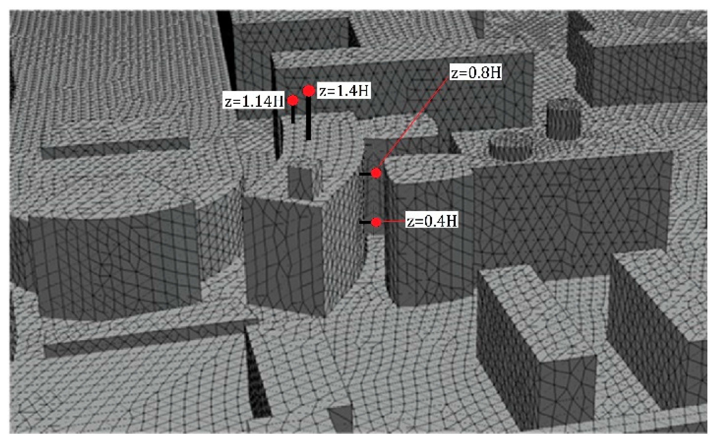
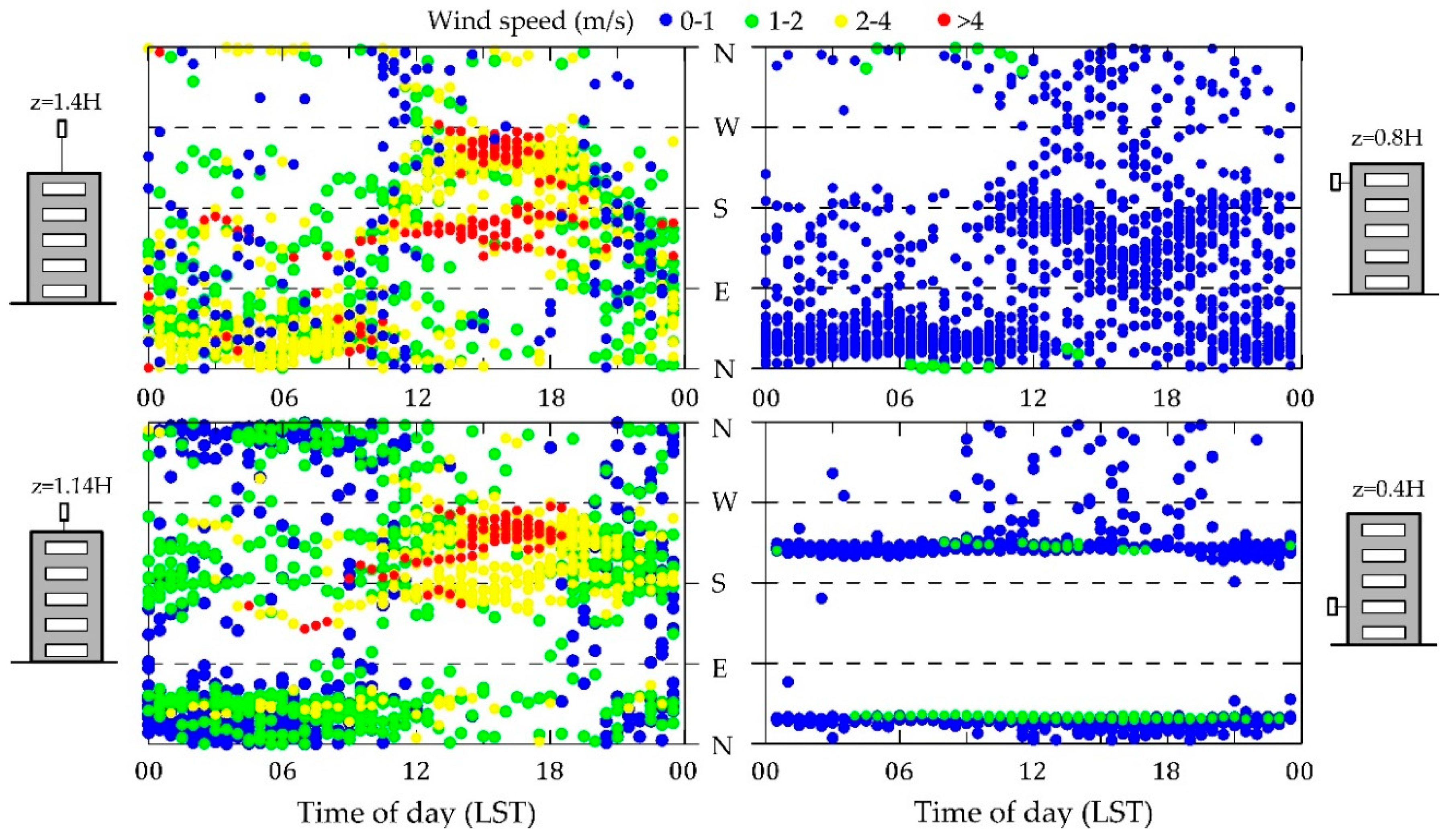
• The CFD simulations and experimental data highlight the profound difference between the airflow above the building and that within the urban canyon. The horizontal wind speed within the canyon was always lower than that above the terrace (on April 2018, 0.35 ms⁻¹, 0.67 ms⁻¹, and 1.83 ms⁻¹ at z = 0.8H, z = 0.4H, and z = 1.14H, respectively). The correlation between the wind speed measured by the two anemometers placed inside the canyon was weak (R² = 0.58), although it was higher than the correlation between the canyon and the terrace (R² = 0.16).
• The vertical gradient of the outdoor UFPs observed in the canyon depended considerably on the season and was about −550 parts/cm³/m in winter, while it was nearly negligible in summer. This is probably due to the larger vertical mixing occurring in summer associated with the convective activity that characterizes the hottest periods.
• Conversely, the vertical gradients of the indoor PM and UFPs measured indoors were dependent on both external and indoor sources.
• The pollen concentrations measured in the suburban environment show a strict relation with occupants’ habits.

Ultimately, these results confirm that indoor particulate matter concentration depends not only on outdoor and indoor sources, but also on the indoor airflow and outdoor microclimate near the considered building.

The results of this project made it possible to make significant steps forward in understanding the mechanisms that regulate air quality in indoor sites, where people spend most of their time, to highlight the peculiar features of crowded environments and to provide a set of data that are essential for assessing the exposure of students and workers in the university and research sectors.

References

1. WHO. WHO Global Strategy on Health, Environment and Climate Change: The Transformation Needed to Improve Lives and Well-Being Sustainably through Healthy Environments; World Health Organization: Geneva, Switzerland, 2020. [Google Scholar]
2. Climate Change and Human Health. Available online: https://www.who.int/globalchange/mediacentre/news/cop23-23-key-messages/en/ (accessed on 15 July 2020).
3. Biswas, P.; Wu, C.-Y. Nanoparticles and the Environment. J. Air Waste Manag. Assoc. 2005, 55, 708–746. [Google Scholar] [CrossRef]
4. Adams, M.D.; Kanaroglou, P.S. Mapping real-time air pollution health risk for environmental management: Combining mobile and stationary air pollution monitoring with neural network models. J. Air Waste Manag. Assoc. 2016, 168, 133–141. [Google Scholar] [CrossRef]
5. Bravo, M.A.; Fuentes, M.; Zhang, Y.; Burr, M.J.; Bell, M.L. Comparison of exposure estimation methods for air pollutants: Ambient monitoring data and regional air quality simulation. Environ. Res. 2012, 116, 1–10. [Google Scholar] [CrossRef] [PubMed] [Green Version]
6. Makri, A.; Stalianakis, N.I. Vulnerability to air pollution health effects. Int. J. Hyg. Environ. Health 2007, 211, 326–336. [Google Scholar] [PubMed]
7. Oakes, M.; Baxter, L.; Long, T.C. Evaluating the application of multipollutant exposure metrics in air pollution health studies. Environ. Int. 2014, 69, 90–99. [Google Scholar] [CrossRef] [Green Version]
8. Ki-Hyun, K.; Kabir, E.; Kabir, S. A review on the human health impact of airborne particulate matter. Environ. Int. 2015, 74, 136–143. [Google Scholar]
9. Anderson, J.O.; Thundiyil, J.G.; Stolbach, A. Clearing the air: A review of the effects of particulate matter air pollution on human health. J. Med. Toxicol. 2012, 8, 166–175. [Google Scholar]
10. Delfino, R.J.; Sioutas, C.; Malik, S. Potential Role of Ultrafine Particles in Associations between Airborne Particle Mass and Cardiovascular Health. Environ. Health Perspect. 2005, 113, 934–946. [Google Scholar]
11. Pope, C.A., III; Dockery, D.W. Health Effects of Fine Particulate Air Pollution: Lines that Connect. J. Air Waste Manag. Assoc. 2006, 56, 709–742. [Google Scholar] [CrossRef]
12. Rückerl, R.; Schneider, A.; Breitner, S.; Cyrys, J.; Peters, A. Health effects of particulate air pollution: A review of epidemiological evidence. Inhal. Toxicol. 2011, 23, 555–592. [Google Scholar]
13. Pope, C.A., III. Epidemiology of fine particulate air pollution and human health: Biologic mechanisms and who’s at risk? Environ. Health Perspect. 2000, 108, 713–723. [Google Scholar] [PubMed]
14. Oh, H.-J.; Kim, J. Monitoring Air Quality and Estimation of Personal Exposure to Particulate Matter Using an Indoor Model and Artificial Neural Network. Sustainability 2020, 12, 3794. [Google Scholar]
15. Kumar, P.; Patton, A.P.; Durant, J.L.; Frey, H.C. A review of factors impacting exposure to PM2.5, ultrafine particles and black carbon in Asian transport 683 microenvironments. Atmos. Environ. 2018, 187, 301–316. [Google Scholar]
16. Burcu, O.; Alver Şahin, Ü.; Burcu, U.; Özcan, A.; Fazilet, Ö.; Coşkun, A. Determinants of exposure to ultrafine particulate matter, black carbon, and PM 2.5 in common travel modes in Istanbul. Atmos. Environ. 2019, 206, 258–270. [Google Scholar] [CrossRef]
17. Kumar, P.; Robins, A.; Vardoulakis, S.; Britter, R. A review of the characteristics of nanoparticles in the urban atmosphere and the prospects for developing regulatory controls. Atmos. Environ. 2010, 44, 5035–5052. [Google Scholar]
18. Guttikunda, S.K.; Goel, R.; Pant, P. Nature of air pollution, emission sources, and management in the Indian cities. Atmos. Environ. 2014, 95, 501–510. [Google Scholar] [CrossRef]
19. Karagulian, F.; Belis, C.A.; Dora, C.F.C.; Prüss-Ustün, A.M.; Bonjour, S.; Adair-Rohani, H.; Amann, M. Contributions to cities’ ambient particulate matter (PM): A systematic review of local source contributions at global level. Atmos. Environ. 2015, 120, 475–483. [Google Scholar]
20. Heal, M.R.; Kumar, P.; Harrison, R.M. Particles, Air Quality, Policy and Health. Chem. Soc. Rev. 2012, 41, 6606–6630. [Google Scholar]
21. Pant, P.; Harrison, R.M. Critical review of receptor modelling for particulate matter: A case study of India. Atmos. Environ. 2012, 49, 1–12. [Google Scholar]
22. Saarikoski, S.; Timonen, H.; Saarnio, K.; Aurela, M.; Järvi, L.; Keronen, P.; Kerminen, V.-M.; Hillamo, R. Sources of organic carbon in fine particulate matter in northern European urban air. Atmos. Chem. Phys. 2008, 8, 6281–6295. [Google Scholar] [CrossRef] [Green Version]
23. Perrino, C.; Tofful, L.; Canepari, S. Chemical characterization of indoor and outdoor fine particulate matter in an occupied apartment in Rome, Italy. Indoor Air 2016, 26, 558–570. [Google Scholar] [CrossRef] [PubMed]
24. Guo, H.; Morawska, L.; He, C.R.; Zhang, Y.L.; Ayoko, G.; Cao, M. Characterization of particle number concentrations and PM2.5 in a school: Influence of outdoor air pollution on indoor air. Environ. Sci. Pollut. Res. Int. 2010, 17, 1268–1278. [Google Scholar] [PubMed] [Green Version]
25. Romagnoli, P.; Balducci, C.; Perilli, M.; Vichi, F.; Imperiali, A.; Cecinato, A. Indoor air quality at life and work environments in Rome, Italy. Environ. Sci. Pollut. Res. Int. 2016, 23, 3503–3516. [Google Scholar] [CrossRef] [PubMed]
26. Li, Z.; Wen, Q.; Zhang, R. Sources, health effects and control strategies of indoor fine particulate matter (PM2.5): A review. Sci. Total Environ. 2017, 586, 610–622. [Google Scholar] [CrossRef] [PubMed]
27. Mandin, C.; Trantallidi, M.; Cattaneo, A.; Canha, N.; Mihucz, V.C.G.; Szigeti, T.; Mabilia, R.; Perreca, E.; Spinazzè, A.; Fossati, S.; et al. Assessment of indoor air quality in office buildings across Europe—The OFFICAIR study. Sci. Total Environ. 2017, 579, 169–178. [Google Scholar] [PubMed] [Green Version]
28. Constantini, S.; Voutsa, D. Size distribution of airborne particulate matter and associated heavy metals in the roadside environment. Chemosphere 2005, 59, 1197–1206. [Google Scholar]
29. Zauli-Sajani, S.; Rovelli, S.; Trentini, A.; Bacco, D.; Marchesi, S.; Scotto, F.; Zigola, C.; Lauriola, P.; Cavallo, D.M.; Poluzzi, V.; et al. Higher health effects of ambient particles during the warm season: The role of infiltration factors. Sci. Total Environ. 2018, 627, 67–77. [Google Scholar] [PubMed]
30. Costabile, F.; Alas, H.; Aufderheide, M.; Avino, P.; Amato, F.; Argentini, S.; Barnaba, F.; Berico, M.; Bernardoni, V.; Biondi, R.; et al. First Results of the “Carbonaceous Aerosol in Rome and Environs (CARE)”. Experiment: Beyond Current Standards for PM10. Atmosphere 2017, 8, 249. [Google Scholar]
31. Zhang, Q.; Canagaratna, M.R.; Jayne, J.T.; Worsnop, D.R. Time- and size-resolved chemical composition of submicron particles in Pittsburgh: Implications for aerosol sources and processes. J. Geophys. Res. Atmos. 2005, 110, D07S09. [Google Scholar] [CrossRef] [Green Version]
32. Lewtas, J. Air pollution combustion emissions: Characterization of causative agents and mechanisms associated with cancer, reproductive, and cardiovascular effects. Mutat. Res. 2007, 636, 95–133. [Google Scholar]
33. Viana, M.; Díez, S.; Reche, C. Indoor and outdoor sources and infiltration processes of PM1 and black carbon in an urban environment. Atmos. Environ. 2011, 45, 6359–6367. [Google Scholar]
34. Quang, T.; He, C.; Morawska, L.; Knibbs, L. Influence of ventilation and filtration on indoor particle concentrations in urban office buildings. Atmos. Environ. 2013, 79, 41–52. [Google Scholar]
35. Chen, C.; Zhao, B. Review of relationship between indoor and outdoor particles: I/O ratio, infiltration factor and penetration factor. Atmos. Environ. 2011, 45, 275–288. [Google Scholar]
36. Buonanno, G.; Fuoco, F.C.; Marini, S.; Stabile, L. Particle Resuspension in School Gyms during Physical Activities. Aerosol Air Qual. Res. 2012, 12, 803–813. [Google Scholar]
37. Koponen, I.K.; Koivisto, A.J.; Jensen, K.A. Worker Exposure and High Time-Resolution Analyses of Process-Related Submicrometre Particle Concentrations at Mixing Stations in Two Paint Factories. Ann. Occup. Hyg. 2015, 59, 749–763. [Google Scholar] [CrossRef]
38. Mosqueron, L.; Momas, I.; Le Moullec, Y. Personal exposure of Paris office workers to nitrogen dioxide and fine particles. Occup. Environ. Med. 2002, 59, 550–556. [Google Scholar] [PubMed] [Green Version]
39. Wilson, W.E.; Mage, D.T.; Grant, L.D. Estimating Separately Personal Exposure to Ambient and Non ambient Particulate Matter for Epidemiology and Risk Assessment: Why and How. J. Air Waste Manag. Assoc. 2000, 50, 1167–1183. [Google Scholar] [CrossRef] [Green Version]
40. Bartyzel, J.; Zięba, D.; Nęcki, J.; Zimnoch, M. Assessment of Ventilation Efficiency in School Classrooms Based on Indoor–Outdoor Particulate Matter and Carbon Dioxide Measurements. Sustainability 2020, 12, 5600. [Google Scholar]
41. Zhong, L.; Yuan, J.; Fleck, B. Indoor Environmental Quality Evaluation of Lecture Classrooms in an Institutional Building in a Cold Climate. Sustainability 2019, 11, 6591. [Google Scholar]
42. Azimi, P.; Zhao, D.; Stephens, B. Estimates of HVAC filtration efficiency for fine and ultrafine particles of outdoor origin. Atmos. Environ. 2014, 98, 337–346. [Google Scholar]
43. Shirzadi, M.; Tominaga, Y.; Mirzaei, P. Experimental study of cross-ventilation of a generic building in highly-dense urban areas: Impact of planar area density and wind direction. J. Wind Eng. Ind. Aerodyn. 2020, 196, 104030. [Google Scholar]
44. Pini, A.; Musa, I.; Monti, P.; Leuzzi, G.; Di Bernardino, A.; Cattani, G.; Di Menno di Bucchianico, A.; Gherardi, M.; Pelliccioni, A. Numerical and experimental analysis of flow and particulate matter dispersion in indoor environment. IOP Conf. Ser. Earth Environ. Sci. 2020, 489, 012007. [Google Scholar] [CrossRef]
45. Peng, Z.; Deng, W.; Tenorio, R. Investigation of Indoor Air Quality and the Identification of Influential Factors at Primary Schools in the North of China. Sustainability 2017, 9, 1180. [Google Scholar]
46. Kalimeri, K.K.; Saraga, D.E.; Lazaridis, V.D.; Legkas, N.A.; Missia, D.A.; Tolis, E.I.; Bartzis, J.G. Indoor air quality investigation of the school environment and estimated health risks: Two-season measurements in primary schools in Kozani, Greece. Atmos. Pollut. Res. 2016, 7, 1128–1142. [Google Scholar] [CrossRef]
47. Tofful, L.; Perrino, C. Chemical composition of indoor and outdoor PM2.5 in three schools in the city of Rome. Atmosphere 2015, 6, 1422–1443. [Google Scholar]
48. Schneider, T.; Alstrup Jensen, K.; Clausen, P.A.; Afshari, A.; Gunnarsen, L.; Wahlin, P.; Glasius, M.; Palmgren, F.; Nielsen, O.J.; Fogh, C.L. Prediction of indoor concentration of 0.5–4 mm particles of outdoor origin in an uninhabited apartment. Atmos. Environ. 2004, 38, 6349–6359. [Google Scholar]
49. Kearney, J.; Wallace, L.; MacNeill, M.; Xu, X.; Van Ryswyk, K.; You, H.; Kulka, R.; Wheeler, A.J. Residential indoor and outdoor ultrafine particles in Windsor, Ontario. Atmos. Environ. 2011, 45, 7583–7593. [Google Scholar] [CrossRef]
50. Schieweck, A.; Uhde, E.; Salthammer, T.; Salthammer, L.C.; Morawska, L.; Mazaheri, M.; Kumar, P. Smart homes and the control of indoor air quality. Renew. Sustain. Energy Rev. 2018, 94, 705–718. [Google Scholar] [CrossRef]
51. Ciardini, V.; Caporaso, L.; Sozzi, R.; Petenko, I.; Bolignano, A.; Morelli, M.; Melas, D.; Argentini, S. Interconnections of the urban heat island with the spatial and temporal micrometeorological variability in Rome. Urban Clim. 2019, 29, 100493. [Google Scholar] [CrossRef]
52. Monti, P.; Leuzzi, G. A Numerical Study of Mesososcale Airflow and Dispersion over Coastal Complex Terrain. Int. J. Environ. Pollut. 2005, 25, 239–250. [Google Scholar] [CrossRef]
53. Petenko, I.; Mastrantonio, G.; Viola, A.; Argentini, S.; Coniglio, L.; Monti, P.; Leuzzi, G. Local circulation diurnal patterns and their relationship with large-scale flows in a coastal area of the Tyrrhenian Sea. Bound. Layer Meteorol. 2011, 139, 353–366. [Google Scholar] [CrossRef]
54. Mastrantonio, G.; Fiocco, G. Accuracy of wind velocity determinations with Doppler sodars. J. Appl. Meteorol. 1982, 21, 823–830. [Google Scholar] [CrossRef]
55. Mastrantonio, G.; Viola, A.P.; Argentini, S.; Fiocco, G.; Giannini, L.; Rossini, L.; Abbate, G.; Ocone, R.; Casonato, M. Observations of sea breeze events in Rome and the surrounding area by a network of Doppler sodars. Bound. Layer Meteorol. 1994, 71, 67–80. [Google Scholar] [CrossRef]
56. Pichelli, E.; Ferretti, R.; Cacciani, M.; Siani, A.M.; Ciardini, V.; Di Iorio, T. The role of urban boundary layer investigated with high-resolution models and ground-based observations in Rome area: A step towards understanding parameterization potentialities. Atmos. Meas. Tech. 2014, 7, 315–332. [Google Scholar] [CrossRef] [Green Version]
57. Ciardini, V.; Di Iorio, T.; Di Liberto, L.; Tirelli, C.; Casasanta, G.; di Sarra, A.; Fiocco, G.; Fuà, D.; Cacciani, M. Seasonal variability of tropospheric aerosols in Rome. Atmos. Res. 2012, 118, 205–214. [Google Scholar] [CrossRef]
58. ANSYS Inc. ANSYS Fluent User’s Guide; ANSYS Inc.: Canonsburg, PA, USA, 2010. [Google Scholar]
59. UNI 11108. Air Quality. Method for Sampling and Counting of Airborne Pollen Grains and Fungal Spores; UNI, Italian National Unification: Milano, Italy, 2004. [Google Scholar]
60. UNI CEN/TS 16868:2015. Ambient Air—Sampling and Analysis of Airborne Pollen Grains and Fungal Spores for Allergy Networks—Volumetric Hirst Method; UNI, Italian National Unification: Milano, Italy, 2015. [Google Scholar]
61. Mandrioli, P. Basic aerobiology. Aerobiologia 1998, 14, 89. [Google Scholar] [CrossRef]
62. Canepari, S.; Perrino, C.; Astolfi, M.L.; Catrambone, M.; Perret, D. Determination of soluble ions and elements in ambient air suspended particulate matter: Inter-technique comparison of XRF, IC and ICP for sample-by-sample quality control. Talanta 2009, 77, 1821–1829. [Google Scholar]
63. Perrino, C.; Catrambone, M.; Dalla Torre, S.; Rantica, E.; Sargolini, T.; Canepari, S. Seasonal variations in the chemical composition of particulate matter: A case study in the Po Valley. Part I: Macrocomponents and mass closure. Environ. Sci. Pollut. Res. 2014, 21, 3999–4009. [Google Scholar]
64. Perrino, C.; Marcovecchio, F. A new method for assessing the contribution of Primary Biological Atmospheric Particles to the mass concentration of the atmospheric aerosol. Environ. Int. 2016, 87, 108–115. [Google Scholar]
65. Pelliccioni, A.; Monti, P.; Leuzzi, G. An alternative wind profile formulation for urban areas in neutral conditions. Environ. Fluid Mech. 2015, 15, 135–146. [Google Scholar] [CrossRef] [Green Version]
66. Pelliccioni, A.; Monti, P.; Leuzzi, G. Wind-speed profile and roughness sublayer modelling in urban boundary layers. Bound. Layer Meteorol. 2016, 160, 225–248. [Google Scholar] [CrossRef]
67. Baik, J.-J.; Kim, J.-J.; Fernando, H.J.S. A CFD model for simulating urban flow and dispersion. J. Appl. Climatol. 2003, 42, 1636–1648. [Google Scholar] [CrossRef]
68. Di Bernardino, A.; Monti, P.; Leuzzi, G.; Querzoli, G. Turbulent Schmidt number measurements over three-dimensional cubic arrays. Bound. Layer Meteorol. 2020, 174, 231–250. [Google Scholar] [CrossRef] [Green Version]
69. Blocken, B.; Stathopoulos, T.; Carmeliet, J.; Hensen, L.M. Application of computational fluid dynamics in building performance simulation for the outdoor environment: An overview. J. Build. Perform. Simul. 2011, 4, 157–184. [Google Scholar] [CrossRef]
70. Garau, M.; Badas, M.G.; Ferrari, S.; Seoni, A.; Querzoli, G. Turbulence and air exchange in a two-dimensional urban street canyon between gable roof buildings. Bound. Layer Meteorol. 2018, 167, 123–143. [Google Scholar] [CrossRef]
71. Cannata, G.; Petrelli, C.; Barsi, L.; Gallerano, F. Numerical integration of the contravariant integral form of the Navier–Stokes equations in time-dependent curvilinear coordinate systems for three-dimensional free surface flows. Contin. Mech. Thermodyn. 2019, 31, 491–519. [Google Scholar] [CrossRef] [Green Version]
72. Franke, J.; Hellsten, A.; Schlùnzen, H.; Carissimo, B. The COST 732 Best Practice Guideline for CFD simulation of flows in the urban environment: A summary. Int. J. Environ. Pollut. 2011, 44, 419–427. [Google Scholar] [CrossRef]
73. Tominaga, Y.; Mochida, A.; Yoshie, R.; Kataoka, R.; Nozu, T.; Yoshikawa, M.; Shirasawa, T. AIJ guidelines for practical applications of CFD to pedestrian wind environment around buildings. J. Wind Eng. Ind. Aerodyn. 2006, 96, 1749–1761. [Google Scholar] [CrossRef]
74. Hirose, C.; Ikegaya, N.; Hagashima, A. Outdoor measurements of relationship between canopy flow and wall pressure distributions of a block within urban-like block array. Build. Environ. 2020, 176, 106881. [Google Scholar] [CrossRef]
75. Nardecchia, F.; Di Bernardino, A.; Pagliaro, F.; Monti, P.; Leuzzi, G.; Gugliermetti, L. CFD analysis of urban canopy flows employing the V2F model: Impact of different aspect ratios and relative heights. Adv. Meteorol. 2018, 2018, 2189234. [Google Scholar] [CrossRef]
76. Wang, L.; Su, J.; Gu, Z.; Shui, Q. Effect of Street Canyon Shape and Tree Layout on Pollutant Diffusion under Real Tree Model. Sustainability 2020, 12, 2105. [Google Scholar] [CrossRef] [Green Version]
77. Di Bernardino, A.; Monti, P.; Leuzzi, G.; Querzoli, G. Pollutant fluxes in two-dimensional street canyons. Urban Clim. 2018, 24, 80–93. [Google Scholar] [CrossRef]
78. Cantelli, A.; Monti, P.; Leuzzi, G. Numerical study of the urban geometrical representation impact in a surface energy budget model. Environ. Fluid Mech. 2015, 15, 251–273. [Google Scholar] [CrossRef]
79. Salizzoni, P.; Soulhac, L.; Mejean, P. Street canyon ventilation and atmospheric turbulence. Atmos. Environ. 2009, 43, 5056–5067. [Google Scholar] [CrossRef]
80. Coceal, O.; Thomas, T.G.; Castro, I.P.; Belcher, S.E. Mean flow and turbulence statistics over groups of urban-like cubical obstacles. Bound. Layer Meteorol. 2006, 121, 491–519. [Google Scholar] [CrossRef]
81. Hoek, G.; Beelen, R.; Kos, G.; Dijkema, M.; van der Zee, S.C.; Fischer, P.H.; Brunekreef, B. Land use regression model for ultrafine particles in Amsterdam. Environ. Sci. Technol. 2011, 45, 622–628. [Google Scholar] [CrossRef]
82. Klompmaker, J.O.; Montagne, D.R.; Meliefste, K.; Hoek, G.; Brunekreef, B. Spatial variation of ultrafine particles and black carbon in two cities: Results from a short-term measurement campaign. Sci. Total Environ. 2015, 508, 266–275. [Google Scholar]
83. Kukkonen, J.; Karl, M.; Keuken, M.P.; Denier van der Gon, H.A.C.; Denby, B.R.; Singh, V.; Douros, J.; Manders, A.; Samaras, Z.; Moussiopoulos, N.; et al. Modelling the dispersion of particle numbers in five European cities. Geosci. Model Dev. 2016, 9, 451–478. [Google Scholar]
84. Cattani, G.; Gaeta, A.; Di Menno di Bucchianico, A.; de Santis, A.; Gaddi, R.; Cusano, M.; Ancona, C.; Badaloni, C.; Forastiere, F.; Gariazzo, C.; et al. Development of land-use regression models for exposure assessment to ultrafine particles in Rome, Italy. Atmos. Environ. 2017, 156, 52–60. [Google Scholar]
85. Salimi, F.; Mazaheri, M.; Clifford, S.; Crilley, L.R.; Laiman, R.; Morawska, L. Spatial variation of particle number concentration in school microscale environments and its impact on exposure assessment. Environ. Sci. Technol. 2013, 47, 5251–5258. [Google Scholar] [CrossRef]
86. Marconi, A.; Cattani, G.; Cusano, M.; Ferdinandi, M.; Inglessis, M.; Viviano, G.; Settimo, G.; Forastiere, F. Two-years of fine and ultrafine particles measurements in Rome, Italy. J. Toxicol. Environ. Health Part A 2007, 70, 213–221. [Google Scholar]
87. Cattani, G.; Di Menno di Bucchianico, A.; Dina, D.; Inglessis, M.; Notaro, C.; Settimo, G.; Viviano, G.; Marconi, A. Evaluation of the temporal variation of air quality in Rome, Italy, from 1999 to 2008. Ann. dell’Istituto Super. Sanità 2010, 46, 242–253. [Google Scholar]
88. McMurry, P.H.; Woo, K.S. Size distributions of 3–100-nm urban Atlanta aerosols: Measurement and observations. J. Aerosol Med. 2002, 15, 169–178. [Google Scholar] [PubMed]
89. Boccuni, F.; Ferrante, R.; Tombolini, F.; Iavicoli, S.; Pelliccioni, A. Measurement of airborne ultrafine particles in work and life environments: Study design and preliminary trends in an Italian university site. IOP Conf. Ser. Mater. Sci. Eng. 2019, 609, 042077. [Google Scholar] [CrossRef] [Green Version]
90. Gariazzo, C.; Pelliccioni, A. A Multi-City Urban Population Mobility Study Using Mobile Phone Traffic Data. Appl. Spat. Anal. Policy 2019, 12, 753–771. [Google Scholar] [CrossRef]
91. Jantunen, J.; Saarinen, K. Intrusion of airborne pollen through open windows and doors. Aerobiologia 2009, 25, 193–201. [Google Scholar] [CrossRef]
92. Farao, C.; Canepari, S.; Perrino, C.; Harrison, R.M. Sources of PM in an Industrial Area: Comparison between receptor model Results and semiempirical calculations of source contributions. Aerosol Air Qual. Res. 2014, 14, 1558–1572. [Google Scholar]
93. Pallarés, S.; Gómez, E.; Martínez, A.; Jordán, M.M. The relationship between indoor and outdoor levels of PM10 and its chemical composition at schools in a coastal region in Spain. Heliyon 2019, 5, e02270. [Google Scholar]
94. Carrion-Matta, A.; Kang, C.M.; Gaffin, J.M.; Hauptman, M.; Phipatanakul, W.; Koutrakis, P.; Gold, D.R. Classroom indoor PM2.5 sources and exposures in inner-city schools. Environ. Int. 2019, 131, 104968. [Google Scholar]
95. Rivas, I.; Viana, M.; Moreno, T.; Bouso, L.; Pandolfi, M.; Alvarez-Pedrerol, M.; Forns, J.; Alastuey, A.; Sunyer, J.; Querol, X. Outdoor infiltration and indoor contribution of UFP and BC, OC, secondary inorganic ions and metals in PM2.5 in schools. Atmos. Environ. 2015, 106, 129–138. [Google Scholar]
96. Oregon Department of Environmental Quality. Draft Recommended Procedures for Toxic Air Contaminant Health Risk Assessments. 2019. Available online: https://www.oregon.gov/ (accessed on 15 July 2020).
97. Nisbet, I.C.; LaGoy, P.K. Toxic equivalency factors (TEFs) for polycyclic aromatic hydrocarbons (PAHs). Regul. Toxicol. Pharmacol. 1992, 16, 290–300. [Google Scholar] [PubMed]
Figure 1. Left picture: Campus of the Sapienza University of Rome (dotted line) and the building of the Physics Department (yellow circle). Right picture: Italian Workers’ Compensation Authority (INAIL) Research Center in Monte Porzio Catone (Rome); the yellow circle indicates the building where the measurements were carried out.
Sustainability 12 09758 g001
Figure 2. Southern view of the Physics Department (PD) and surrounding buildings showing the positions of the sonic anemometers (z = 1.14H: terrace; z = 0.4H and z = 0.8H: east facade). z = 1.4H refers to the Sonic Detection and Ranging (SODAR) range gate considered for the analysis. The grid in the picture is that used in the computational fluid dynamics (CFD) simulations.
Sustainability 12 09758 g002
Figure 3. Study area and sampling points; routes followed for itinerant measurements.
Sustainability 12 09758 g003
Figure 4. Thirty-minute averages of the wind direction as a function of the time of day measured by the Sonic Detection and Ranging (SODAR; z = 1.4H) and the three anemometers installed on the PD building (April 2018). Colors indicate wind speed.
Sustainability 12 09758 g004
Figure 5. Left panel: horizontal wind speed map at z = 0.4H simulated at 16:00 local standard time (LST) on 21 April 2018. Right panel: as in the left panel, but for the pressure field. The dark gray and the black features denote the PD and the Chemistry Department, respectively.
Sustainability 12 09758 g005
Figure 6. Average particle number concentration (PNC) values at the measurement points selected in the study area (left panel: winter campaign, right panel: summer campaign). A: inside the university campus; B: main roads on the perimeter outside the university campus; C: urban area 3B—San Lorenzo.
Sustainability 12 09758 g006
Figure 7. Average 24 h daily trends of total PNC (#/cm3) in the size range 5.6–560 nm: Terrace (blue line, z = 1.1H, from 13 November to 17 November), computer room (CR) (orange line, z = 0.4H, from 20 November to 24 November), and LH (black line, z = 0.1H, from 27 November to 1 December).
Sustainability 12 09758 g007
Figure 8. Daily trends of pollen concentration and occupants’ presence during working days and non-working days for two representative periods of the monitoring campaign: (a) 20 June–17 July 2016 and (b) 18 July–14 August 2016.
Sustainability 12 09758 g008
Figure 9. Trend of pollen concentrations during working hours and non-working hours of representative days during the winter campaign (26 January–21 February 2017) in relation to mean occupants (a), mean door openings (b), and mean window openings (c). The dotted lines refer to 07:30 and 19:30 LST.
Sustainability 12 09758 g009
Figure 10. Mass closure (left panels) and macro-sources (left panels) of PM10 collected outdoors (upper panels) and inside a classroom (lower panels) during the period 26 November–9 December 2018.
Sustainability 12 09758 g010
Figure 11. Image of indoor bioaerosol through an optical microscope (montage of ten fields).
Sustainability 12 09758 g011