Volatility in Rainfall and Predictability of Droughts in Northwest Bangladesh


1
Department of Statistics, Faculty of Science, University of Dhaka, Dhaka 1000, Bangladesh
2
Department of Disaster Science and Management, Faculty of Earth and Environmental Sciences, University of Dhaka, Dhaka 1000, Bangladesh
3
School of Civil Engineering, Faculty of Engineering, Universiti Teknologi Malaysia (UTM), Johor Bahru 81310, Malaysia
4
Faculty of Civil Engineering, Seoul National University of Science and Technology, Seoul 01811, Korea
*
Authors to whom correspondence should be addressed.
Sustainability 2020, 12(23), 9810; https://0-doi-org.brum.beds.ac.uk/10.3390/su12239810
Submission received: 7 September 2020
/
Revised: 9 November 2020
/
Accepted: 21 November 2020
/
Published: 24 November 2020
(This article belongs to the Special Issue Climate Change Impacts on Hydrology, Water Quality and Ecology)
Abstract
:This study was conducted to evaluate the variability, trends, volatility, and transition patterns of rainfall in drought-prone northwest Bangladesh. Daily rainfall recorded at five stations for the period 1959–2018 were used for this purpose. Non-parametric tests of variability changes, a modified Mann–Kendall trend test, innovative trend analysis (ITA), a generalized autoregressive conditional heteroscedasticity (GARCH)–jump model, and a Markov chain (MC) were used to assess the variability changes, trends, volatility, and transitions in rainfall to understand the possibility of the persistence of droughts and their predictability. The results showed an overall decrease of variability in annual and seasonal rainfall, but an increase in mean pre-monsoon rainfall and a decrease in mean monsoon rainfall. This caused a decrease in pre-monsoon droughts, but few changes in monsoon droughts. The ITA and rainfall anomaly analysis revealed high temporal variability and, thus, rapid shifts in rainfall regimes, which were also supported by the volatility dynamics and time-varying jumps from the GARCH–jump model and the rapid changes in drought index from the MC analysis. Therefore, the lack of drought in recent years cannot be considered as an indicator of declining droughts in the region.
1. Introduction
Increased atmospheric water vapor in warmer climates has altered the seasonal and geographical variability of rainfall [1,2], which has consequently changed the probability of rainfall extremes and hydrological disasters like floods and droughts [3]. Higher implications of a warmer climate have been found for droughts compared to other hydrological disasters [4,5,6,7] Droughts mainly affect agriculture and, thus, the livelihoods of millions of people who are dependent on agricultural production every year [8,9,10]. Globally, economic loss due to droughts is four times higher than that incurred from floods [11]. Therefore, changes in droughts can have severe implications for society and the economy.
The impacts of climate change on precipitation and droughts are different in different regions. More recurrent and intense droughts have been noticed in recent years all over the globe [4,12,13,14,15,16,17]. At the same time, an increase in rainfall reliability and, thus, lessening of droughts have also been reported in some regions [18,19]. This indicates a large spatial heterogeneity in drought trends on a global scale. The Intergovernmental Panel on Climate Change (IPCC) [20] also reported a large spatial variability in drought trends. That is, there have been more frequent droughts in the Mediterranean and western Africa and less in central northern America and northwestern Australia. In addition, different changes in different characteristics of droughts in the same regions have been reported. Liu et al. [21] reported the increasing recurrence but decreasing duration of droughts in the Haihe River basin of China. Shiru et al. [14] found that droughts covering large areas are decreasing, but localized droughts with a smaller areal coverage are increasing in Nigeria.
Contradictory results in drought trends have also been reported for South Asia. Dai [4] reported increasing dryness in South Asia over the period 1950–2008, while Mishra et al. [19] found decreasing frequency and severity of soil moisture droughts in India in recent years. A shift in droughts has also been noticed in Bangladesh with the changes in rainfall variability [22]. Several studies reported a possible increase in droughts in the country due to climate change [23,24]. However, the recent statistics of the Bangladeshi government indicated a reduction of droughts in the last three decades. The analysis of recent climate data also revealed that the general conception of at least two droughts per decade is no longer valid for the country. However, it is often argued that the recent subsidence of droughts is a temporal phenomenon that does not indicate a reduction of drought frequency in Bangladesh. The existing uncertainty in drought trends emphasizes the need for further analysis of rainfall patterns to make a factual conclusion. Assessment of the predictability of droughts based on analysis of intrinsic rainfall characteristics can provide an understanding of the possible continuation of recent subsiding trends in droughts.
The predictability of a time series depends on the amount of information in the past series that continues into the present series [25]. A series is easily predictable if the past information is conveyed to the present. The measurement of the intrinsic predictability of a series is required to understand the continuation of information in the series. If a series is predictable, then it can be considered that a forecast based on the present condition is also valid for the near future. Several methods have been proposed to measure time series predictability, including estimation of loss functions [26], analysis of information [27], estimation of univariate and multivariate volatility [28], assessment of stationarity [29], and estimation of transition probability [30].
Among all the methods, the estimation of volatility is the most widely used for evaluating the predictability of a time series. High volatility in rainfall means that a rainfall anomaly can change regimes in a short period [31] and cause floods or droughts at any time [32]. Several studies have been conducted in recent years to assess volatility in rainfall and possible changes in hydrological hazards. Swain et al. [33] reported an increase in the probability of a rapid shift between wet and dry episodes in many regions of the globe due to an increase in rainfall volatility. Nijsse et al. [34] also reported an increase in climatic extremes due to an increase in the volatility of the global climate. Assessment of transition probability is another newly adopted method for estimation of predictability. A Markov chain (MC) [35] is generally used for this purpose, where the sequence of climate states is analyzed to understand the climate regime shifts or unpredictability [36,37]. In recent years, it has been used for assessment of possible future shifts in rainfall regimes and the occurrence of droughts [38,39,40].
The objective of the present study is to assess the volatility of rainfall and the shifting of rainfall regimes to understand the possible changes in the probability of occurrence of droughts in northwest Bangladesh. Sixty years of daily rainfall data recorded at five locations in the northwest drought-prone area of Bangladesh were used for this purpose. Non-parametric methods were used for the assessment of changes in mean and variability of rainfall and droughts. In addition, innovative trend analysis (ITA) was used to assess the time-varying changes in rainfall in Bangladesh. The generalized autoregressive conditional heteroscedasticity (GARCH)—jump model [30] was used to estimate the volatility of rainfall, and the MC was used to assess the probability of a shift in drought proneness. The novelty of the study is the application of GARCH—jumps and Markov chain for the analysis of the predictability of droughts. The results can indicate whether the recent subsidence of droughts in Bangladesh is a reduction of droughts or if it is a temporary subsidence, after which the country may be affected by droughts again in the near future. The findings of the study can help disaster risk mitigation policy planning. The procedure used in this study for the systematic analysis of rainfall data with robust statistical methods can be replicated for analysis of the predictability of any other climatic phenomena in Bangladesh or any other regions.
2. Study Area and Data
2.1. Geography and Climate of the Study Area
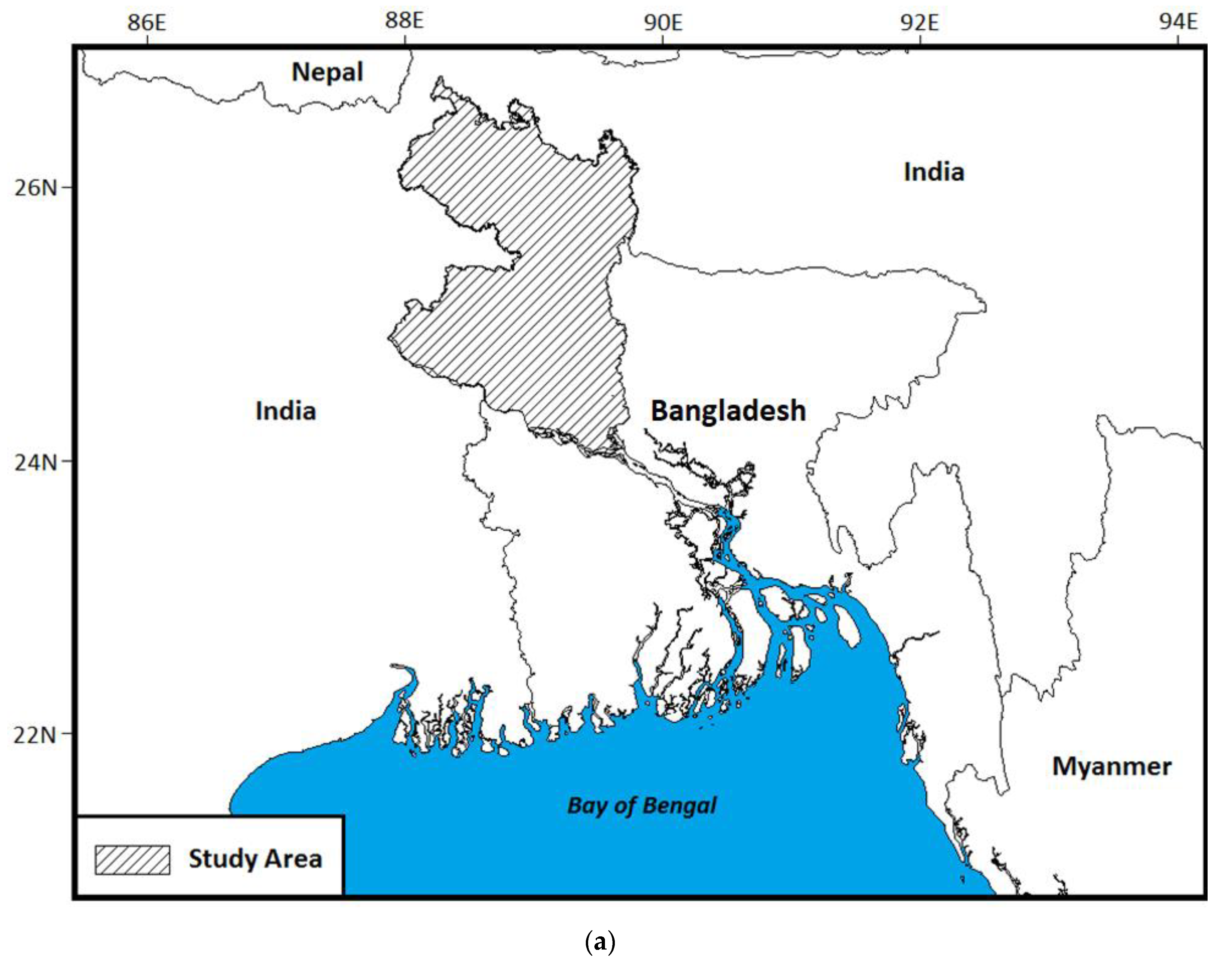
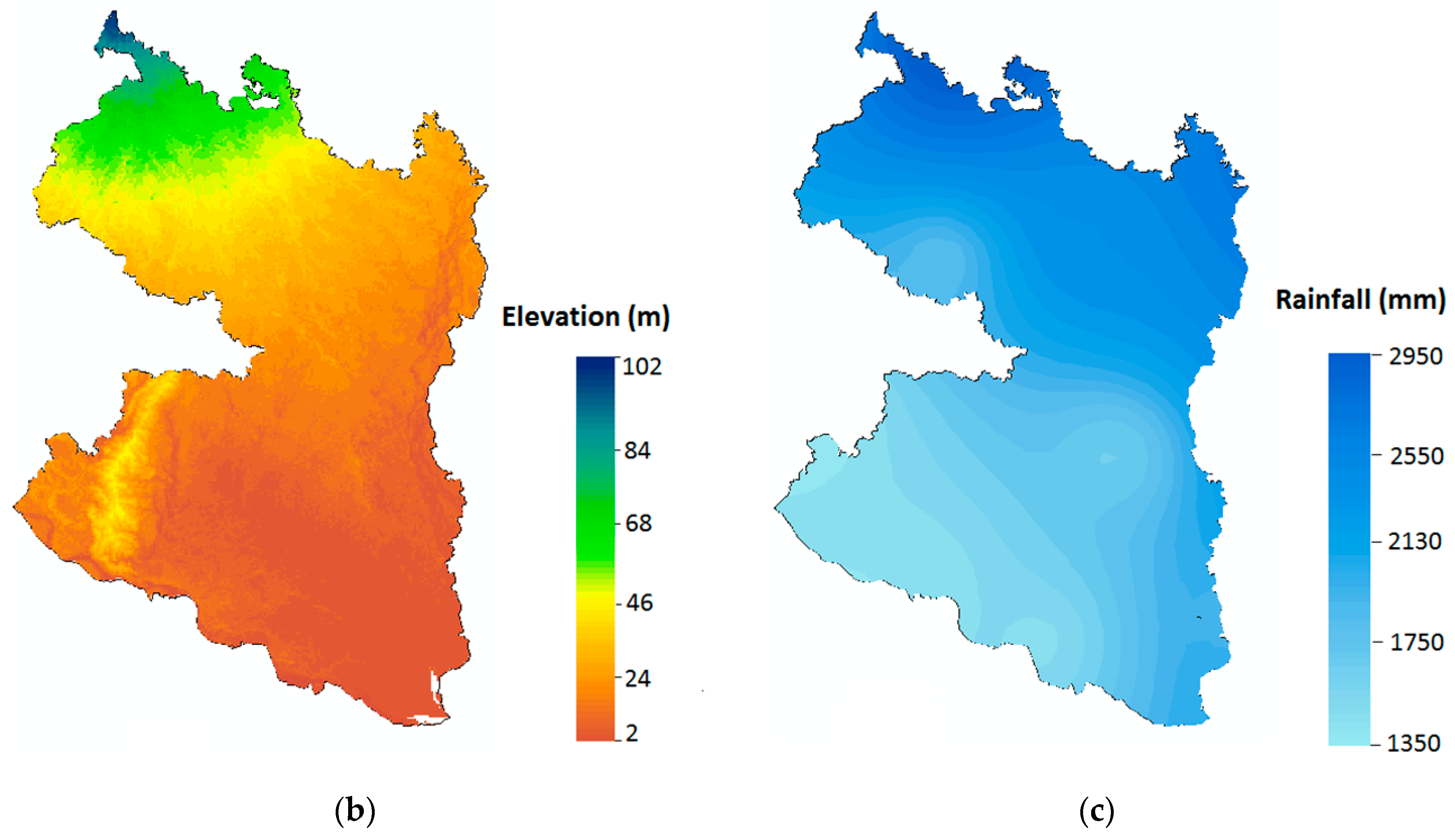
The study area consisted of the north and northwest districts of Bangladesh and covered an area of 34,359 km2. The location of the study area on the map of Bangladesh is shown in Figure 1. The topography of the region is very flat, except for a mildly uplifted land in the southwest (Figure 1b). There is a slight gradient from the north to the south. The annual rainfall map of the study area (Figure 1c) was prepared by interpolating the annual average rainfall estimated at five meteorological stations in the study area using the inverse distance weighting method. The annual rainfall in the study area varies from 1350 mm in the southwest to nearly 2950 mm in the far north (Figure 1c). The monthly mean of daily maximum temperature in the region varies from 25.4 °C in January to 35.9 °C in April, and the minimum temperature ranges between 10.2 °C in January and 26.2 °C in August. The climate of the study area can be divided into four seasons: winter (December–February), pre-monsoon (March–May), monsoon (June–September), and post-monsoon (October–November) [41]. The seasonal variability of rainfall in the area is very high. About 60% of the rainfall occurs in the monsoon season and less than 3% occurs in winter. The annual variability of rainfall is also high; therefore, droughts are recurrent phenomena in the region. On average, droughts occur twice in a decade in the region.
2.2. Data and Sources
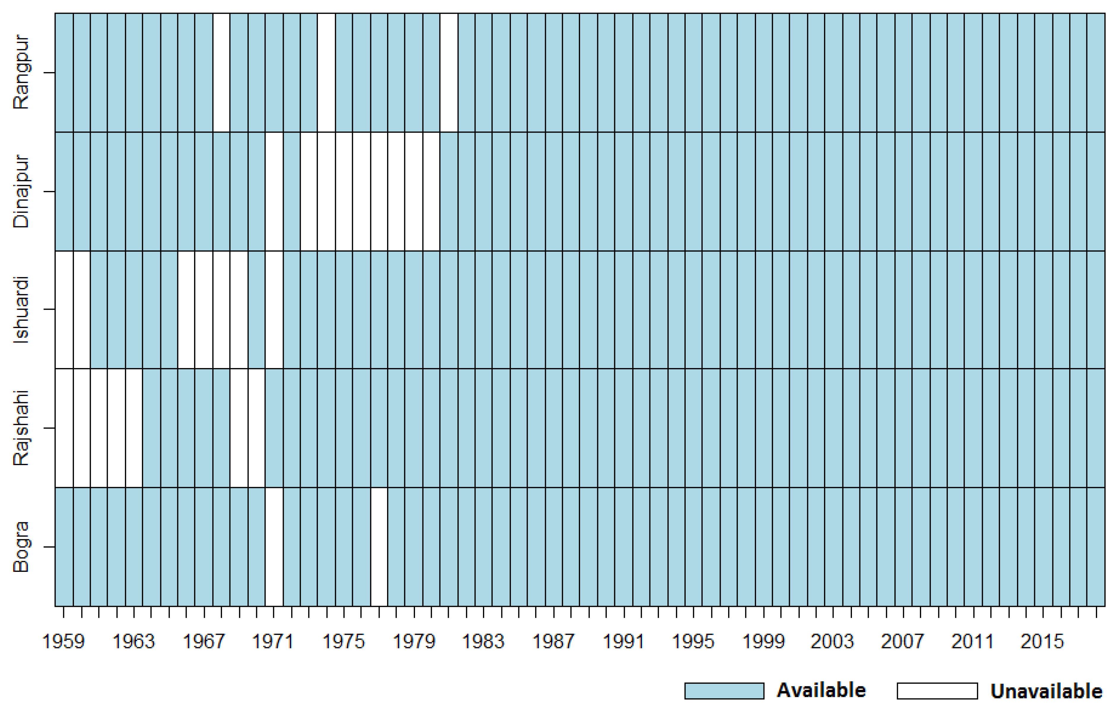
Daily rainfall data recorded at five meteorological stations in the study area for the period 1959–2018 were collected from the Bangladesh Meteorological Department. The rainfall data of Bangladesh contain many missing records. If rainfall of a year was found missing for more than 2%, the whole record for the year was removed. The data available at different stations are shown in Figure 2.
Both subjective and objective approaches were used for the assessment of the quality of rainfall records. Initial screening was performed through data inspection, such as for negative values, no rainfall in monsoon months, more than 50 mm rainfall in winter months, etc. Rainfall data were also used to generate a time series plot and histogram for each station to detect any inconsistency [42]. In addition, a double mass curve was prepared for annual rainfall for all the stations to reveal any break in data series. Finally, a sequential student t-test was conducted to test any difference among different subsets of rainfall data [43].
No inconsistency was observed in the rainfall time series and histograms, nor were breaks in the double mass curves at any station. No abnormal values were noticed during data inspection and numerical checking. Student’s t-test revealed no differences between any two subsets of rainfall data. Therefore, the quality of collected rainfall records was considered sufficient for the different statistical analyses performed in this study.
3. Methodology
The procedure used to assess the possible changes in the probability of drought occurrence in northwest Bangladesh is outlined below:
- Non-parametric variance tests were conducted to assess changes in rainfall variability between the early (1959–1988) and late (1989–2018) periods.
- Sen’s slope estimator and the Mann–Kendall trend test were used to evaluate the changes in annual and seasonal rainfall over the study period (1959–2018) and their significance, respectively.
- ITA was conducted for visual inspection of time-varying changes in rainfall.
- The standardized precipitation index (SPI) was computed for the assessment of droughts during monsoon and pre-monsoon months.
- Trend analysis was used to evaluate the changes in seasonal droughts.
- The GARCH—jumps model was used to estimate the volatility of rainfall to evaluate the frequency of rainfall change between wet and dry regimes.
- The MC was used to assess the probability of transition of rainfall from wet to dry states for understanding the possibility of future droughts.
Details of the methods used in this study are described in the following sections.
3.1. Changes in Variability in Monthly Rainfall
Rainfall variability is the major factor that determines the occurrence of droughts. More droughts occur more in regions where rainfall variability is high. A decrease in rainfall variability indicates a decrease in the probability of occurrence of droughts and vice versa. The coefficient of variability is often used to measure variability in rainfall, while different statistical tests are used to measure the changes in variability between two periods. In this study, Levene’s test [44] and Barlett’s test [45] were used to reveal any changes in variability in monthly rainfall. The rainfall data were equally divided into two periods (1959–1988 and 1989–2018), and the tests were conducted between rainfall data of those two periods to evaluate the changes in variability in monthly rainfall.
The coefficient of variability (CV%) in monthly rainfall for all months of a year and the months for a season can be estimated using the following equation:
where μ and σ are the mean and standard deviation of rainfall.
Levene’s test is a non-parametric test used to verify the difference in variances between two sets of data. This method estimates the spread of data from the sample median to assess differences in variance between two sets of data. It is considered as a robust test due to its independence from underlying data distribution [46,47]. Levene’s test statistic is defined as:
where is the number of different groups to which the sampled cases belong, is the number of cases in the th group, is the total number of cases in all groups, represents the average of for group , and is the average of all .
The Barlett test is applicable where the variances are based on equal or unequal numbers in the degree of freedom. Bartlett’s test is more sensitive to data distribution than Levene’s test. Barlett’s test calculations are based on the corrected Chi-Square, which can be expressed as
where is the variance, is the degrees of freedom for each group, and is the number of groups being compared.
3.2. Changes in Rainfall and Droughts
The rate of change in rainfall or drought index was estimated using Sen’s slope (SS) estimator, and the significance of the change was estimated using a modified version of the Mann–Kendall (i.e., MMK) test. In addition, ITA was employed for graphical assessment of trends to evaluate changes in trends over the study period. The SS estimator, MMK tests, and ITA methods are elaborated below.
3.2.1. Sen’s Slope (SS) Estimator
The non-parametric SS estimator [48] estimates the rate of change () as the median of the slopes () of all the consecutive pairs of data,
where and are data values at times j and k, respectively.
3.2.2. Modified Mann–Kendal (MMK) Test
The MMK test [49,50] was used to assess the significance of the changes estimated using the SS estimator. The MK test estimates the significance of the change using Z statistics,
where
The null hypothesis of ‘no trend’ is rejected at the 0.05 significance level (p < 0.05) if is out of the range of ±1.96.
The significance of the Mann–Kendall (MK) test is affected by autocorrelation in data series, which is common in rainfall data [51,52,53,54]. Therefore, the MMK test introduced by Yue et al. [55] through a trend-free pre-whitening (PW) method was adopted in this study. The PW is performed using the following equation:
where represents Theil–Sen’s slope of different pairs of data. The final series () by removing autocorrelation () is estimated using Equations (7) and (8).
The MK test is conducted over the time series of to avoid any influence of autocorrelation in trend significance.
3.2.3. Innovative Trend Analysis
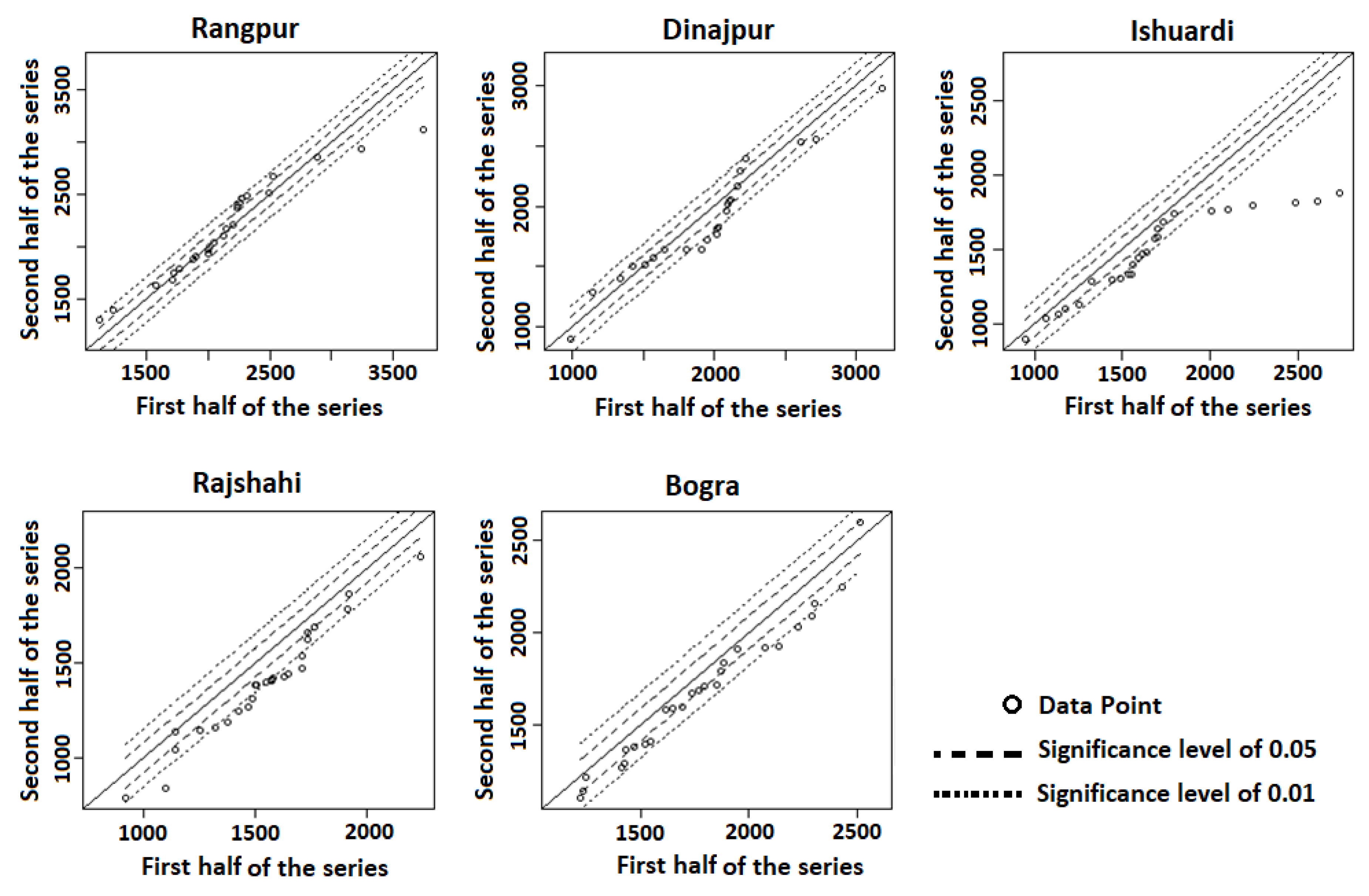
ITA allows an analysis of trends or no trends in various parts of time series through visual examination of data; therefore, it can be utilized for the recognition of sub-trends [3,10,54,56]. In ITA, the data series is divided into two sub-series ( and ) of the same sample size (n) ordered ascendingly. A scatter plot is then drawn from the two sub-series. The data points above or below the diagonal line of the plot specify rising or declining trends, respectively. The ITA trend statistic, is estimated as it was by Sen [57]:
where and are the means of two sub-series. The confidence interval (CI) of the trend at a significance α is estimated from the standard deviation () of SITA as
When the points in the scatter plot cross the CL, the hypothesis of ‘no trend’ is rejected.
3.3. Rainfall Anomaly
Rainfall anomalies were estimated based on discrete rainfall anomalies (DRAs) and the rainfall anomaly index (RAI) [58]. DRAs for annual and seasonal scales are estimated as the deviation of annual or seasonal rainfall of each year from the mean of annual or seasonal rainfall for the entire period. The estimation of the RAI is based on the mean of the ten highest () precipitation records for the study period, as shown below:
where is the mean precipitation for the whole study period and P is a specific precipitation record. Dry and wet years can be categorized based on the RAI, as given in Table 1.
3.4. Standardized Precipitation Index
The SPI [59] is estimated as the probability of rainfall for a period in months compared to the same period in other years. Rainfall data are generally fitted using a probability distribution function (PDF) for estimating the SPI [60,61]. A previous study reported gamma as the best PDF for fitting the rainfall of Bangladesh [62]. The fitting of the gamma distribution to rainfall (x) can be expressed as
where α, β, and Γ(α) represent the shape, scale, and gamma function. The α, β, and Γ(α) of the gamma PDF are estimated for different time scales of interest, e.g., one, three, or more months, for estimating droughts for different durations. The parameter values are used to estimate the cumulative probability of a rainfall amount over a defined period in terms of the whole period as
The gamma function cannot be defined for zero rainfall, and therefore, the cumulative probability becomes
where q represents the probability of zero rainfall. The drought is categorized according to the SPI, as presented in Table 2. The standard probability of occurrence of a certain category of droughts is also presented in Table 2 [63].
3.5. Generalized Autoregressive Conditional Heteroscedasticity (GARCH)
The GARCH [40] model was used for the assessment of rainfall volatility and jumping behavior. The heteroscedasticity or unequal variance of rainfall may exhibit autocorrelation, which means that a conditional variance depends on past variances [64]. The GARCH model estimates a serial dependency of volatility and includes the past rainfall in estimating future volatility [65]. The GARCH model first defines the conditional mean equation as follows:
where denotes the logarithmic difference of rainfall data at time t, and is the error that follows either a normal or Student’s t distribution. The GARCH (1,1) model introduced by Engle [66] and Bollerslev [40] takes the following form:
where refers to conditional variance at time t, and indicates the volatility at time t − 1.
For the assessment of jumping behavior, Jorion [67] proposed a GARCH model with jumps, as shown below:
where is the log change of rainfall at time t, is a constant of autoregression (AR), [AR(2)] represents the returns, and is the error at time t, which has two components,
where is a mean-zero innovation with the normal stochastic process
Hence, the volatility of follows a standard GARCH (1,1) process.
The second component, can be used to define the inconsistency between the jump component and the anticipated total jump size ( between t − 1 and t,
where represents the jump size, which has a normal distribution with a mean and variance of and , respectively, and represents the jump component with the number of jumps, . Considering that follows a Poisson distribution, the jump intensity can be presented as
where is the conditional jump intensity parameter, and . The log-likelihood function can be presented as , where are the model parameter vectors of Equations (16)–(20). The interpretation of rainfall volatility is made based on the values of these parameters.
3.6. Markov Chain
An MC was used to assess the irregular transition of rainfall and its impacts on dryness or wetness. If the probability of wetness of a period (e.g., week) only depends on the wetness of the previous period, it can be expressed as random variables X0, X1, …, Xn, distributed identically, where
The MC is estimated for different steps and the dryness index is developed considering the transition matrix:
where = ). Note that + = 1 and + = 1. Here, means the probability of the next week being wet if the present week is wet. Using Equation (22), a higher transition probability matrix can be calculated to estimate a dryness index as [68]:
The dryness index (DI) can have a value in the range of 0 to 1. A higher value of DI indicates a lower degree of dryness. The susceptibility of an area to drought can be defined based on the DI value, as shown in Table 3.
4. Results and Discussions
4.1. Changes in Rainfall Variability
The coefficients of variability in monthly rainfall during the early (1959–1988) and late (1989–2018) periods were estimated and statistical tests were conducted to evaluate the significance in the difference of variability between the two periods. The obtained results are presented in Table 4. A significant change in variability from both Levene’s and Barlett’s tests is marked using a bold font in the table. The tests were conducted annually and for the, monsoon and pre-monsoon seasons. These two seasons were considered as nearly 85% of the total annual rainfall occurs during these two seasons. Any deficit of rainfall during these two seasons causes damage to the agriculture of the country.
The results revealed a significant decrease in annual rainfall variability at three out of five stations in the study area. The decreases in monsoon and pre-monsoon rainfall variabilities were observed at one and three stations, respectively. The results revealed more reliability in both annual and seasonal rainfalls in northwest Bangladesh in recent years compared to the early period.
4.2. Trends in Rainfall in Bangladesh
Trends in annual and seasonal rainfall at different locations of northwest Bangladesh for the period 1959–2018 are presented in Table 5. The values in the table represent the rate of rainfall change in mm/decade. The bold numbers indicate significant change at p < 0.05. The results revealed a significant increase in pre-monsoon rainfall at four stations and a decrease at one station. The monsoon rainfall was noticed to decrease at four stations and annual rainfall at two out of the five stations. Overall, the results revealed decreases in annual and monsoon rainfall and an increase in pre-monsoon rainfall in the region.
ITA was conducted for visual inspection of trends over the period and their significance. The ITA of annual rainfall for the period 1959–2018 for the five stations is presented in Figure 3. The figure shows that data points are below the diagonal line for the higher values and above the diagonal line for lower values. The higher values also exceeded the confidence interval lines below the diagonal line. This indicates a decreasing trend in annual rainfall at a significance level of p < 0.05 in recent years at most of the stations. The trends were significantly positive or insignificant in the early years. The results indicate that the large decrease of rainfall in most stations in recent years has caused the overall decrease in rainfall for the entire study period, as detected by the MK test.
4.3. Trends in Droughts in Bangladesh
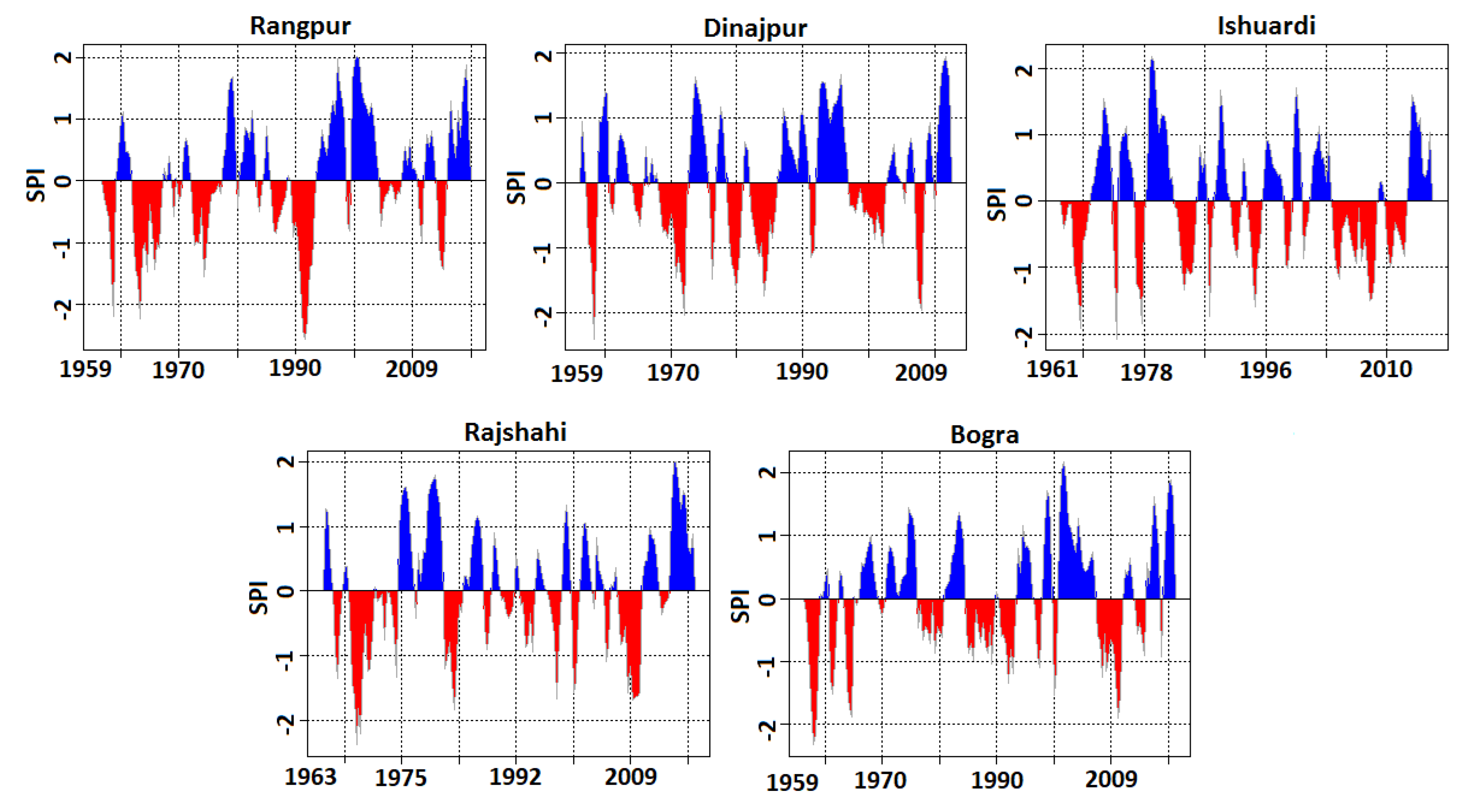
Droughts in Bangladesh are mostly seasonal. Droughts for a long period (e.g., annual scale) do not occur in Bangladesh, like most of the tropical countries. Therefore, only droughts during monsoon and pre-monsoon months were considered in this study. It should be noted that the crops in Bangladesh are cultivated mostly during these two periods. The SPI was estimated for four- and three-month periods to evaluate droughts during the monsoon (June to September) and pre-monsoon (March to May) seasons, respectively. The time series of the three-month SPI at five locations are shown in Figure 4. The SPI values presented using the blue color indicate wet periods, while the SPI values presented using the red color indicate drought periods. The figure shows a random variability of the SPI in the study area. There is no specific pattern in dry and wet periods. However, a gradual decline of SPI peaks during drought years was noticed in almost all stations. The SPI value in the last month of a season was separated to assess the changes in drought in that season. For example, the three-month SPI value of May indicates the rainfall deficit from March to May, and was therefore used to estimate the changes in pre-monsoon droughts. Similarly, the four-month SPI value of September was used to assess the changes in monsoon droughts.
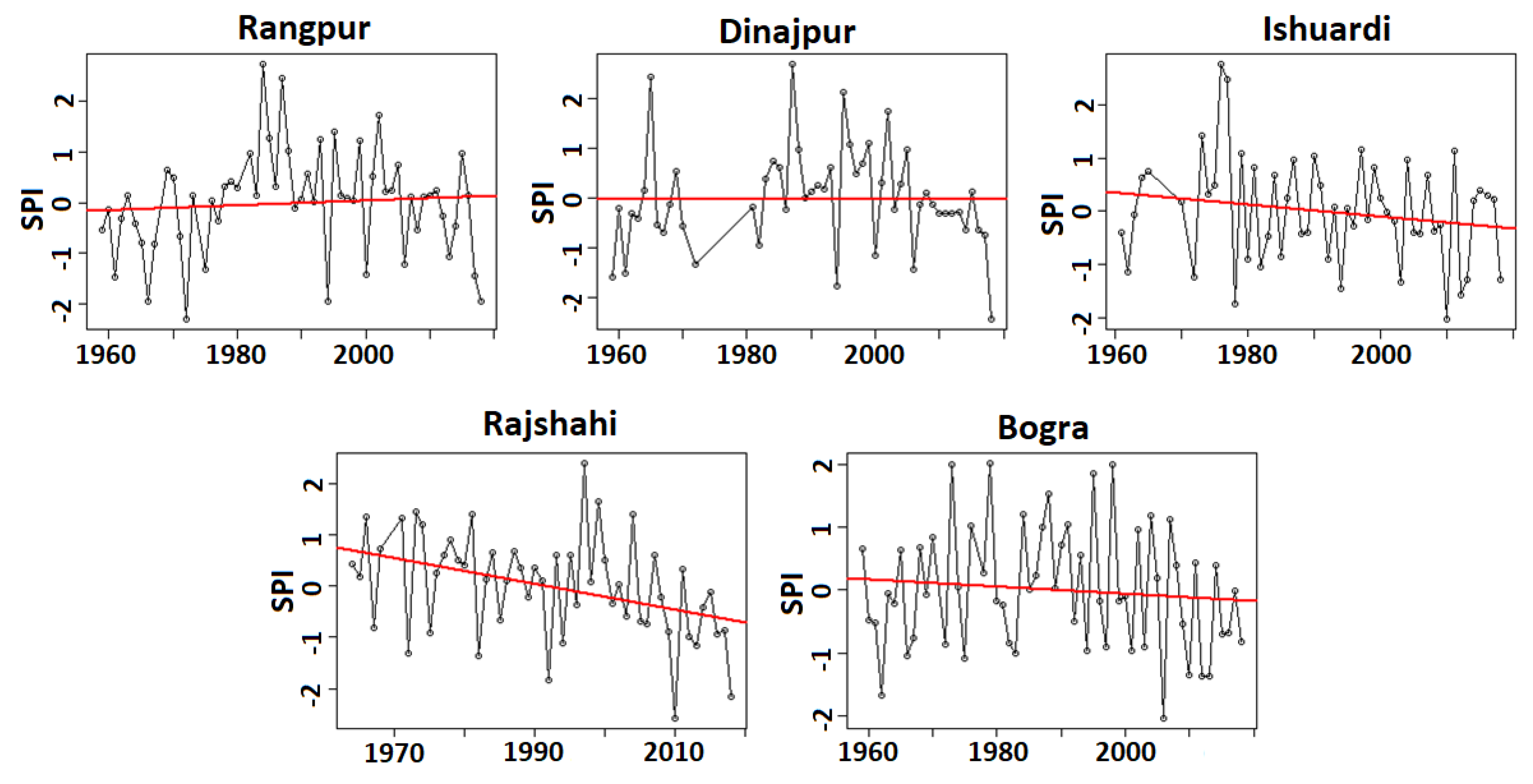
The time series of the monsoon SPI for the five study locations are shown in Figure 5. The MMK trend test was used to assess the changes in the SPI to understand the changing patterns of droughts. The obtained results are also presented in Figure 5. The trend lines are shown using a red line over the SPI time series in the figure. The rate of change of the monsoon SPI per decade is provided in Table 6. The bold numbers in the table represent a significant change. The results show a decrease in the SPI or an increase in droughts at a significance level of 0.05 at two out of the five stations.
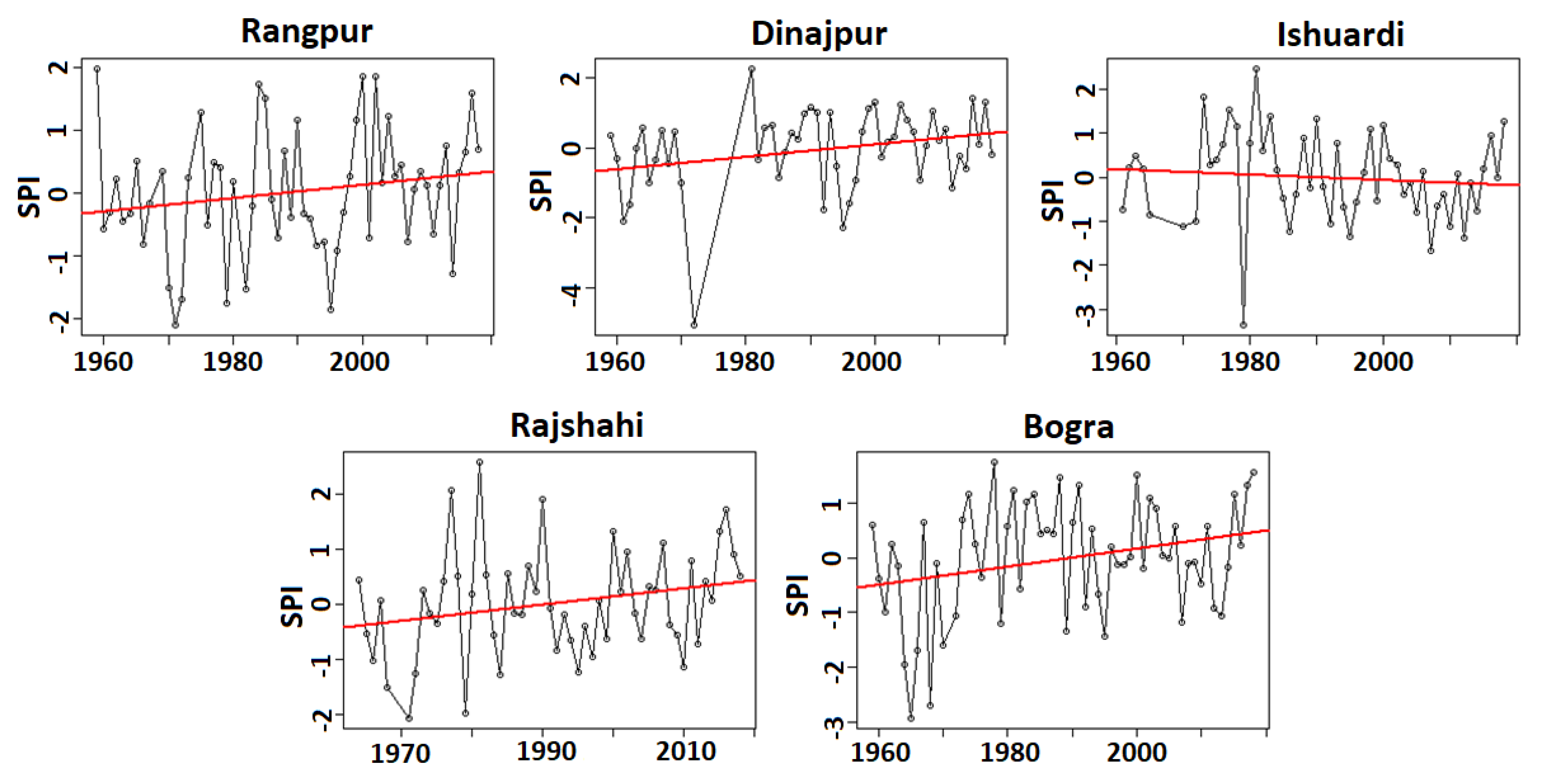
The time series of the pre-monsoon SPI for the study locations are presented in Figure 6, and the rate of change of the pre-monsoon SPI is presented in Table 6. The pre-monsoon drought was found to decrease (increase in SPI values) at four out of five stations, while it was found to increase at one station at a significance level of 0.05. The rainfall in pre-monsoon months was found to increase at the locations where drought was noticed to decrease, while the rainfall was found to decrease at the locations where drought was noticed to increase. The variability in pre-monsoon rainfall was found to decrease at three locations, including the station where the drought was increasing. Therefore, it can be remarked that changes in mean monsoon rainfall may be linked to the changes in droughts in the study area. The increase or decrease in mean pre-monsoon rainfall in recent years has influenced the calculation of rainfall deficit for recent years. This resulted in higher values of the SPI in later periods and an increasing trend in the SPI.
A similar interpretation can be made for monsoon droughts, as the droughts were found to increase at the stations where monsoon rainfall was found to decrease. However, the results were not consistent for all the stations. A decrease in monsoon rainfall was noticed at four out of the five stations, while the increase in monsoon droughts was noticed only at two out of four stations where monsoon rainfall was decreasing. The results indicate that the analysis of variability and the assessment of trends are not enough for a complete understanding of the causes of change in droughts. In addition, such analyses are not enough to understand whether the decreasing trend in droughts will persist in the near future or if there will be a rainfall regime shift that would alter drought trends.
The pre-monsoon rainfall in Bangladesh occurs due to thunderstorms, which are controlled by land surface temperature, and the moist air comes from the Bay of Bengal (BoB) toward the inland [69]. The higher surface temperature has caused an increase in convective available potential energy (CAPE) in the northwest part of the Indian subcontinent [70]. This has caused an increase in thunderstorms in Bangladesh in recent years [71]. The increased thunderstorms have caused an increase in pre-monsoon rainfall in the study area. The monsoons in the study area come from two directions, one from the west part of India and the other from the BoB [72]. The variability in winds from the BoB plays a major role in the changes in the monsoon rainfall of Bangladesh. Vishnu et al. [73] reported a decreasing trend in the number of monsoon depressions in the BoB due to rapid warming of the sea surface. This caused a weakening of monsoon circulation and a decrease in monsoon rainfall in many regions of the Indian subcontinent.
4.4. Annual and Seasonal Rainfall Anomalies
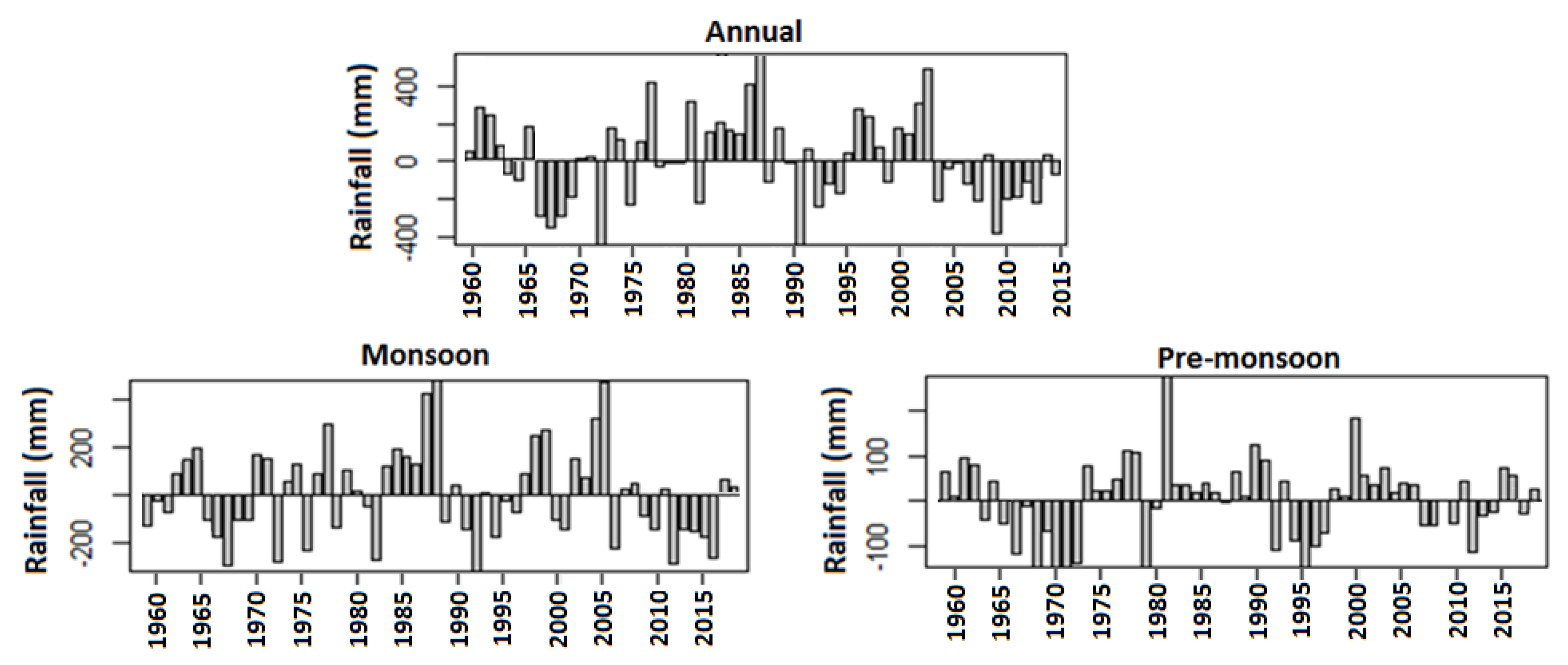
Discrete seasonal rainfall anomalies were calculated as the deviation of the mean seasonal rainfall of each year from its long-term mean. The rainfall anomalies averaged for the study area over the period 1959–2018 are presented in Figure 7. The discrete rainfall anomalies showed that seasonal and annual rainfall fluctuate frequently over time due to the high variability in rainfall. Since the negative rainfall anomalies indicate droughts, it is evident that the drought condition also fluctuates significantly due to the high variability and instability in rainfall.
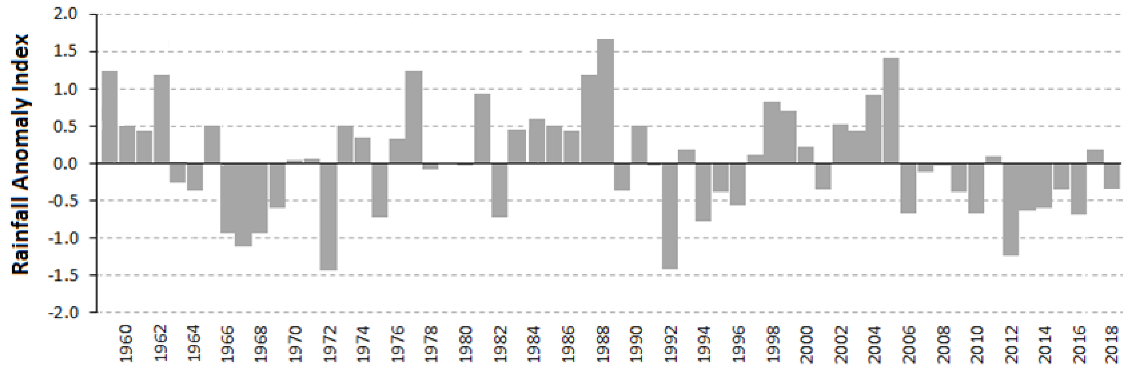
To verify whether high anomalies in the rainfall create droughts, RAI values for different years were estimated. The RAI time series averaged for the study area for the period 1959–2018 is shown in Figure 8. It was observed that the RAI fluctuates significantly over time like the rainfall. However, there is no consistency or apparent pattern in variation. The seasonal RAI values were also calculated, and similar random fluctuations were observed. Therefore, it can be remarked that high variability of rainfall has made the droughts less predictable in northwest Bangladesh.
4.5. Volatility in Rainfall and Instability in Droughts
To verify the visual interpretation of the lower predictability of droughts in the previous sections, the volatility and jumping behaviors of rainfall were estimated using the GARCH-jump model. The assessment was conducted for pre-monsoon and monsoon rainfall, and the results are presented in Table 7. The results revealed that the jump parameters are significant for both pre-monsoon and monsoon seasons, suggesting the existence of major jumps during these two periods. This is expected, as the country experiences more rainfall during these two seasons.
Table 7 shows that parameters ω, α, β, and θ are significant for both seasons. This indicates significant volatility in the time series (ω). The significant value of α indicates that the volatility results from a random variability of rainfall. The significant value of β indicates that the volatility will persist with time and, therefore, rainfall variability is unpredictable for the study area. A significant jump in the rainfall series (θ) was also noticed, which indicates that a shift in the rainfall regime from wet to dry or vice versa can occur at any time.
The results also revealed that the jump intensity parameter is statistically significant for both pre-monsoon and monsoon seasons, implying that the jump intensity varies over time. Since , it can be confirmed that the GARCH-jump model was correctly chosen for describing the jump behavior of the rainfall. These findings reconfirm the fact that dry and wet conditions in northwest Bangladesh fluctuate due to the volatile nature of the rainfall.
4.6. Erratic Transitions in Rainfall and Rapid Fluctuation in Drought Proneness
Finally, an MC model was developed to evaluate the transition behavior of rainfall and to develop the drought proneness index. The model was developed considering weekly rainfall less than 5 mm as a dry week and more than 5 mm as a wet week. This threshold was used to compare the wetness/dryness of the present week with the wetness/dryness of the previous week to estimate transition counts for the Markov model. In the same way, the transition probabilities for the next step were computed based on the dependency of the wetness/dryness condition of the present week on the rain status of two weeks before.
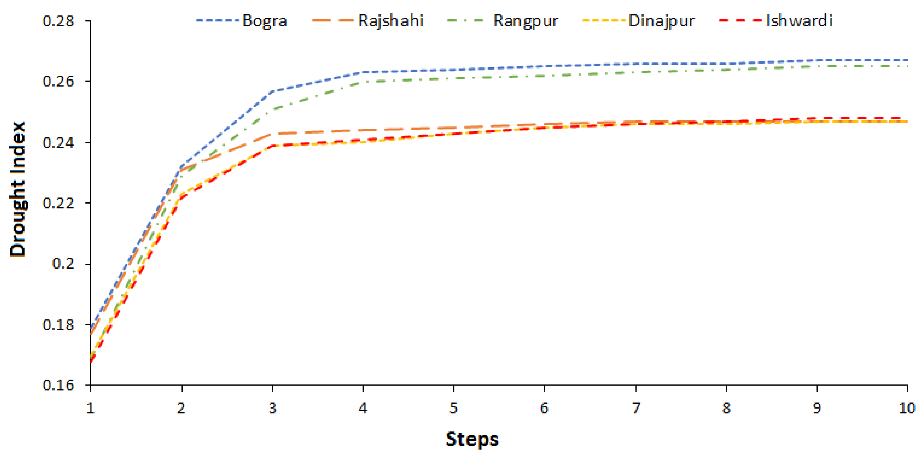
Similarly, higher-order transition probabilities (up to the 10th step) were calculated for the calculation of the DI. The changes in DI values over the transition steps for different stations are presented in Figure 9. The figure shows that the DI gradually becomes stable with time. For example, the DI values at Bogra were 0.179 for the first step, which indicates severe drought. It became a moderate drought (DI = 0.232) in the second step and a mild drought (DI = 0.257) in the third step. The DI values were noticed to increase gradually, and they became stable at 0.267 after the ninth step. Similar changes were noticed at other stations. The results revealed that the DI value changes significantly within a short period. This again proves that the variability of rainfall has made the drought condition rapidly vary with time. High variability in rainfall has made the droughts unpredictable in the study area.
Though droughts are mostly measured on a monthly scale, they often cannot be captured using monthly rainfall in a humid tropical region. Usually, no rainfall for consecutive eight days can affect rain-fed crops in Bangladesh [39]; this is not possible to evaluate using monthly rainfall data. Therefore, the DI was estimated on a weekly scale to understand the predictability of droughts in Bangladesh.
5. Conclusions
This study attempted to assess the variability, trends, anomalies, volatility, and transitions of rainfall in the drought-prone northwest region of Bangladesh for better insight into the causes of drought occurrence, the possibility of their persistence, and scope of their predictability. The results revealed a significant decrease in pre-monsoon droughts in northwest Bangladesh, which is mainly due to a reduction of rainfall variability. No significant change in monsoon droughts was noticed, although the variability of monsoon rainfall was noticed to decrease in recent years (1989–2018) compared to the early period (1959–1988). This is mainly due to a decrease in monsoon rainfall, which kept the ratio of variability stable over time. The ITA revealed a fluctuation of trends in different parts of the study period. Analysis of rainfall anomalies and the RAI also revealed a rapid shift in the rainfall regime from a wet to dry or a dry to wet state in a short period. This was also validated by the GARCH-jump model and MC analysis. The results indicate that the present trend of declining droughts may not persist for a longer period. The high volatility and rapid shifting in the nature of the rainfall have made the predictability of droughts highly uncertain in the region. The rainfall in the region can shift rapidly from a longer wet phase to a severe dry phase, triggering droughts in the region. The study also indicates that droughts in the study area are highly random and, therefore, can occur at any time. These conclusions are based on the results obtained through the analysis of rainfall data of five meteorological stations. In future, the available rainfall records of other locations in the study area can be used to verify the results and understand the spatial variability of drought predictability. In addition, other time series predictability assessment methods, such as estimation of the loss function or changes in entropy, can also be used to verify these study results.
Author Contributions
Conceptualization, M.A.U., A.M.K., S.S., and E.-S.C.; Supervision A.M.K.; Data analysis, M.A.U. and S.S.; Writing—original draft preparation, M.A.U., A.M.K., and S.S.; writing—review and editing, S.S. and E.-S.C. All authors have read and agreed to the published version of the manuscript.
Funding
This study was also supported by a grant (NRF-2016R1D1A1B04931844) from the National Research Foundation of Korea.
Acknowledgments
We are thankful to the anonymous reviewers and editors for their helpful comments and suggestions.
Conflicts of Interest
The authors declare no conflict of interest.
References
- Shahid, S.; Alamgir, M.; Wang, X.; Eslamian, S. Climate Change Impacts on and Adaptation to Groundwater. In Handbook of Drought and Water Scarcity: Environmental Impacts and Analysis of Drought and Water Scarcity, 1st ed.; Eslamian, S., Eslamian, F., Eds.; CRC Press: Boca Raton, FL, USA, 2017; pp. 108–120. [Google Scholar]
- Wang, X.; Zhang, J.; Shamsuddin, S. Impacts of climate variability and changes on domestic water use in the Yellow River Basin of China. Mitig. Adapt. Strateg. Glob. Chang. 2017, 22, 595–608. [Google Scholar] [CrossRef]
- Pour, S.H.; Wahab, A.K.A.; Shahid, S.; Asaduzzaman, M.; Dewan, A. Low impact development techniques to mitigate the impacts of climate-change-induced urban floods: Current trends, issues and challenges. Sustain. Cities Soc. 2020, 62, 102373. [Google Scholar] [CrossRef]
- Dai, A. Drought Under Global Warming: A Review. Wiley Interdiscip. Rev. Clim. Chang. 2011, 2, 45–65. [Google Scholar] [CrossRef] [Green Version]
- Ahmed, K.; Shahid, S.; Harun, S.; Wang, X.J. Characterization of seasonal droughts in Balochistan Province. Pak. Stoch. Environ. Res. Risk Assess. 2016, 30, 747–762. [Google Scholar] [CrossRef]
- Mohsenipour, M.; Shahid, S.; Chung, E.; Wang, X. Changing pattern of droughts during cropping seasons of Bangladesh. Water Resour. Manag. 2018, 32, 1555–1568. [Google Scholar] [CrossRef]
- Qutbudin, I.; Sanusi, M.; Shiru, S.; Sharafati, A.; Ahmed, K.; Al-Ansari, N.; Yaseen, Z.M.; Shahid, S.; Xiaojun Wang, X. Seasonal drought pattern changes due to climate variability: Case study in Afghanistan. Water 2019, 11, 1096. [Google Scholar] [CrossRef] [Green Version]
- Sharafati, A.; Nabaei, S.; Shahid, S. Spatial assessment of meteorological drought features over different climate regions in Iran. Int. J. Climatol. 2019, 40, 1864–1884. [Google Scholar] [CrossRef]
- Sediqi, M.N.; Shiru, M.S.; Nashwan, M.S.; Ali, R.; Abubaker, S.; Wang, X.N.; Ahmed, K.; Shahid, S. Spatio-Temporal Pattern in the Changes in Availability and Sustainability of Water Resources in Afghanistan. Sustainability 2019, 11, 5836. [Google Scholar] [CrossRef] [Green Version]
- Pour, S.H.; Wahab, A.K.A.; Shahid, S. Spatiotemporal changes in aridity and the shift of drylands in Iran. Atmos. Res. 2020, 233, 104704. [Google Scholar] [CrossRef]
- Damania, R.; Desbureaux, S.; Hyland, M.; Islam, A.; Moore, S.; Rodella, A.-S.; Russ, J.; Zaveri, E. Uncharted Waters: The New Economics of Water Scarcity and Variability, 1st ed.; World Bank: Washington, DC, USA, 2017. [Google Scholar]
- Spinoni, J.; Vogt, J.; Naumann, G.; Barbosa, P.; Dosio, A. Will Drought Event Become More Frequent and Severe in Europe? Int. J. Climatol. 2018, 38, 1718–1736. [Google Scholar] [CrossRef] [Green Version]
- Marvel, K.; Cook, B.I.; Céline, J.W.; Durack, P.J.; Smerdon, J.E.; Williams, A.P. Twentieth-century hydroclimate changes consistent with human influence. Nature 2019, 569, 59–65. [Google Scholar] [CrossRef] [PubMed]
- Shiru, M.; Shahid, S.; Alias, N.; Chung, E.-S. Trend analysis of droughts during crop growing seasons of Nigeria. Sustainability 2018, 10, 871. [Google Scholar] [CrossRef] [Green Version]
- Ahmed, K.; Shahid, S.; Sachindra, D.A.; Nawaz, N.; Chung, E.S. Fidelity assessment of general circulation model simulated precipitation and temperature over Pakistan using a feature selection method. J. Hydrol. 2019, 573, 281–298. [Google Scholar] [CrossRef]
- Bi, S.; Lu, Y.; Qu, Y.; Zhao, F. Temporal and spatial characteristics of droughts and floods in northern china from 1644 to 1911. J. Earth Syst. Sci. 2019, 128, 98. [Google Scholar] [CrossRef] [Green Version]
- Chattopadhyay, N.; Malathi, K.; Tidke, N.; Attri, S.D.; Ray, K. Monitoring agricultural drought using combined drought index in india. J. Earth Syst. Sci. 2020, 129, 155. [Google Scholar] [CrossRef]
- Ficklin, D.L.; Maxwell, J.T.; Letsinger, S.L.; Gholizadeh, H. A climatic deconstruction of recent drought trends in the United States. Environ. Res. Lett. 2015, 10, 44009–44018. [Google Scholar] [CrossRef]
- Sung, J.H.; Chung, E.S.; Shahid, S. Reliability-resiliency-vulnerability approach for drought analysis in South Korea using 28 GCMs. Sustainability 2018, 10, 3043. [Google Scholar] [CrossRef] [Green Version]
- IPCC. Contribution of Working Groups I, II and III to the Fifth Assessment Report of the Intergovernmental Panel on Climate Change. In Climate Change 2014: Synthesis Report; Pachauri, R.K., Meyer, L.A., Eds.; IPCC: Geneva, Switzerland, 2014. [Google Scholar]
- Liu, B.; Yan, Z.; Sha, J.; Li, S. Drought Evolution Due to Climate Change and Links to Precipitation Intensity in the Haihe River Basin. Water 2017, 9, 878. [Google Scholar] [CrossRef] [Green Version]
- Mortuza, M.R.; Moges, E.; Demissie, Y.; Li, H.-Y. Historical and future drought in Bangladesh using copula-based bivariate regional frequency analysis. Theor. Appl. Climatol. 2018, 135, 1–17. [Google Scholar] [CrossRef]
- Miyan, M.A. Droughts in Asian Least Developed Countries: Vulnerability and sustainability. Weather Clim. Extrem. 2015, 7, 8–23. [Google Scholar] [CrossRef] [Green Version]
- Ahammed, S.J.; Chung, E.S.; Shahid, S. Parametric assessment of pre-monsoon agricultural water scarcity in Bangladesh. Sustainability 2018, 10, 819. [Google Scholar] [CrossRef] [Green Version]
- Delsole, T. Predictability and Information Theory. Part I: Measures of Predictability. J. Atmos. Sci. 2004, 61, 2425–2440. [Google Scholar] [CrossRef]
- Laurent, S.; Rombouts, J.V.K.; Violante, F. On loss functions and ranking forecasting performances of multivariate volatility models. J. Econom. 2013, 173, 1–10. [Google Scholar] [CrossRef] [Green Version]
- Zhou, R.; Yang, C.; Wan, J.; Zhang, W.; Guan, B.; Xiong, N. Measuring Complexity and Predictability of Time Series with Flexible Multiscale Entropy for Sensor Networks. Sensors 2017, 17, 787. [Google Scholar] [CrossRef] [PubMed] [Green Version]
- Li, X.; Zakamulin, V. Stock volatility predictability in bull and bear markets. Quant. Financ. 2020, 20, 1149–1167. [Google Scholar] [CrossRef] [Green Version]
- Du, H.; Zhao, Z.; Xue, H. ARIMA-M: A New Model for Daily Water Consumption Prediction Based on the Autoregressive Integrated Moving Average Model and the Markov Chain Error Correction. Water 2020, 12, 760. [Google Scholar] [CrossRef] [Green Version]
- Yeh, H.-F.; Hsu, H.-L. Using the Markov Chain to Analyze Precipitation and Groundwater Drought Characteristics and Linkage with Atmospheric Circulation. Sustainability 2019, 11, 1817. [Google Scholar] [CrossRef] [Green Version]
- Yusof, F.; Kane, I.L.; Yusop, Z. Structural break or long memory: An empirical survey on daily rainfall data sets across Malaysia. Hydrol. Earth Syst. Sci. 2013, 17, 1311–1318. [Google Scholar] [CrossRef] [Green Version]
- Swain, D.L.; Langenbrunner, B.; Neelin, J.D. Increasing precipitation volatility in twenty-first-century California. Nat. Clim. Chang. 2018, 8, 427–433. [Google Scholar] [CrossRef]
- Nijsse, F.J.; Cox, P.M.; Huntingford, C.; Williamson, M.S. Decadal global temperature variability increases strongly with climate sensitivity. Nat. Clim. Chang. 2019, 9, 598–601. [Google Scholar] [CrossRef]
- Brémaud, P. Markov Chains: Gibbs Fields, Monte Carlo Simulation and Queues; Springer: New York, NY, USA, 1999. [Google Scholar]
- Rezaeianzadeh, M.; Stein, A.; Cox, J.P. Drought Forecasting using Markov Chain Model and Artificial Neural Networks. Water Resour. Manag. 2016, 30, 2245–2259. [Google Scholar] [CrossRef]
- Rahmat, S.N.; Jayasuriya, N.; Bhuiyan, M.A. Short-term droughts forecast using Markov chain model in Victoria, Australia. Theor. Appl. Climatol. 2017, 129, 445–457. [Google Scholar] [CrossRef]
- Khadr, M. Forecasting of meteorological drought using Hidden Markov Model (case study: The upper Blue Nile river basin, Ethiopia). Ain Shams Eng. J. 2016, 7, 47–56. [Google Scholar] [CrossRef] [Green Version]
- Avilés, A.; C’elleri, R.; Solera, A.; Paredes, J. Probabilistic forecasting of drought events using markov chain and bayesian network-based models: A case study of anandean regulated river basin. Water 2016, 8, 37. [Google Scholar] [CrossRef]
- Selvaraju, R.; Baas, S. Climate Variability and Change: Adaptation to Drought in Bangladesh: A Resource Book and Training Guide; Food and Agriculture Organization of the United Nations: Rome, Italy, 2007; ISBN 978-92-5-105782-7. [Google Scholar]
- Bollerslev, T. Generalized Autoregressive Conditional Heteroscedasticity. J. Econom. 1986, 31, 307–327. [Google Scholar] [CrossRef] [Green Version]
- Pour, S.H.; Shahid, S.; Chung, E.-S.; Wang, X.-J. Model output statistics downscaling using support vector machine for the projection of spatial and temporal changes in rainfall of Bangladesh. Atmos. Res. 2018, 213, 149–162. [Google Scholar] [CrossRef]
- Pour, S.H.; Wahab, A.K.A.; Shahid, S. Changes in reference evapotranspiration and its driving factors in peninsular Malaysia. Atmos. Res. 2020, 246, 105096. [Google Scholar] [CrossRef]
- You, Q.L.; Kang, S.C.; Aguilar, E.; Pepin, N.; Flugel, W.A.; Yan, Y.P. Changes in daily climate extremes in China and their connection to the large scale atmospheric circulation during 1961–2003. Clim. Dyn. 2011, 36, 2399–2417. [Google Scholar] [CrossRef]
- Levene, H. Robust tests for equality of variances. In Contributions to Probability and Statistics: Essays in Honor of Harold Hotelling; Olkin, I., Ed.; Stanford University Press: Stanford, CA, USA, 1960; pp. 278–292. [Google Scholar]
- Bartlett, M.S. Properties of sufficiency and statistical tests. Proc. Roy. Soc. 1937, 160, 268–282. [Google Scholar]
- Khan, M.S.; Coulibaly, P.; Dibike, Y. Uncertainty analysis of statistical downscaling methods using Canadian Global Climate Model predictors. Hydrol. Process. 2006, 20, 3085–3104. [Google Scholar] [CrossRef]
- Awadallah, A.G.; ElGamal, M.; ElMostafa, A.; ElBadry, H. Developing Intensity-Duration-Frequency Curves in Scarce Data Region: An Approach using Regional Analysis and Satellite Data. Engineering 2011, 3, 215–226. [Google Scholar] [CrossRef] [Green Version]
- Sen, P.K. Estimates of the regression coefficient based on Kendall’s tau. J. Am. Stat. Assoc. 1968, 63, 1379–1389. [Google Scholar] [CrossRef]
- Mann, H.B. Nonparametric tests against trend. Econometrica 1945, 13, 245–259. [Google Scholar] [CrossRef]
- Kendall, M.G. Rank Correlation Methods; Griffin: Oxford, UK, 1948. [Google Scholar]
- Khan, N.; Pour, S.H.; Shahid, S. Spatial distribution of secular trends in rainfall indices of Peninsular Malaysia in the presence of long-term persistence. Meteorol. Appl. 2019, 26, 655–670. [Google Scholar] [CrossRef]
- Nashwan, M.S.; Shahid, S.; Rahim, N. Unidirectional trends in annual and seasonal climate and extremes in Egypt. Theor. Appl. Climatol. 2019, 136, 457–473. [Google Scholar] [CrossRef]
- Pour, S.H.; Wahab, A.K.A.; Shahid, S.; Wang, X.J. Spatial pattern of the unidirectional trends in thermal bioclimatic indicators in Iran. Sustainability 2019, 11, 2287. [Google Scholar] [CrossRef] [Green Version]
- Pour, S.H.; Wahab, A.K.A.; Shahid, S. Spatiotemporal changes in precipitation indicators related to bioclimate in Iran. Theor. Appl. Climatol. 2020, 141, 99–115. [Google Scholar] [CrossRef]
- Yue, S.; Pilon, P.; Cavadias, G. Power of the Mann–Kendall and Spearman’s rho tests for detecting monotonic trends in hydrological series. J. Hydrol. 2002, 259, 254–271. [Google Scholar] [CrossRef]
- Girma, A.; Qin, T.; Wang, H. Study on Recent Trends of Climate Variability Using Innovative Trend Analysis: The Case of the upper Huai River Basin. Polish J. Environ. Stud. 2020, 29, 2199–2210. [Google Scholar] [CrossRef]
- Sen, Z. An innovative trend analysis methodology. J. Hydrol. Eng. 2012, 17, 1042–1046. [Google Scholar] [CrossRef]
- Van Rooy, M.P. A Rainfall Anomaly Index independent of time and space. Notos 1965, 14, 43–48. [Google Scholar]
- McKee, T.B.; Doesken, N.J.; Kleist, J. Relationship of Drought Frequency and Duration to Time Scales. In Proceedings of the Eighth Conference on Applied Climatology, Boston, MA, USA, 17–22 January 1993; American Meteorological Society: Boston, MA, USA; pp. 179–184. [Google Scholar]
- Thom, H.C.S. A Note on the Gamma Distribution. Mon. Wea. Rev. 1958, 86, 117–122. [Google Scholar] [CrossRef]
- Edwards, D.C.; McKee, T.B. Characteristics of 20th century drought in the United States at multiple scales. Atmos. Sci. Pap. 1997, 634, 1–30. [Google Scholar]
- Alamgir, M.; Shahid, S.; Hazarika, M.K.; Nashrrullah, S.; Harun, S.B.; Shahid, S. Analysis of meteorological drought pattern during different climatic and cropping seasons in Bangladesh. J. Am. Water Resour. Assoc. 2015, 51, 794–806. [Google Scholar] [CrossRef]
- Moreira, E.E.; Coelho, C.A.; Paulo, A.A.; Pereira, L.S.; Mexia, J.T. SPI-based drought category prediction using loglinear models. J. Hydrol. 2008, 354, 116–130. [Google Scholar] [CrossRef] [Green Version]
- Enders, W. Applied Econometric Time Series; Wiley Series in Probability and Statistics; Wiley: New York, NY, USA, 2004. [Google Scholar]
- Bollerslev, T.; Engle, R.F.; Nelson, D. ARCH Models. In Handbook of Econometrics, 4th ed.; Engle, R., McFadden, D., Eds.; Elsevier Science: Amsterdam, The Netherlands, 1994; pp. 2959–3038. [Google Scholar]
- Engle, R.F. Autoregressive Conditional Heteroscedasticity with Estimates of the Variance of United Kingdom Inflation. Econometrica 1982, 50, 987–1007. [Google Scholar] [CrossRef]
- Jorion, P. On jump processes in the foreign exchange and stock markets. Rev. Financ. Stud. 1988, 1, 427–445. [Google Scholar] [CrossRef]
- Banik, P.; Mandal, A.; Rahman, M.S. Markov chain analysis of weekly rainfall data in determining drought-proneness. Discret. Dyn. Nat. Soc. 2002, 7, 231–239. [Google Scholar] [CrossRef]
- Shahid, S. Recent trends in the climate of Bangladesh. Clim. Res. 2010, 42, 185–193. [Google Scholar] [CrossRef] [Green Version]
- Glazer, R.; Torres–Alavez, J.A.; Coppola, E.; Das, S.; Ashfaq, M.; Sines, T. Projected changes to Severe Thunderstorm environments as a result of 21st century warming from RegCM CORDEX–CORE simulations. EGU Gen. Assem. 2020, 2020, 970. [Google Scholar]
- Wahiduzzaman, M.; Islam, A.R.M.T.; Luo, J.; Shahid, S.; Uddin, M.J.; Shimul, S.M.; Sattar, M.A. Trends and Variabilities of Thunderstorm Days over Bangladesh on the ENSO and IOD Timescales. Atmosphere 2020, 11, 1176. [Google Scholar] [CrossRef]
- Shahid, S. Trends in extreme rainfall events of Bangladesh. Theor. Appl. Climatol. 2011, 104, 489–499. [Google Scholar] [CrossRef]
- Vishnu, S.; Francis, P.A.; Sheno, S.S.C.; Ramakrishna, S.S.S. On the decreasing trend of the number of monsoon depressions in the Bay of Bengal. Environ. Res. Lett. 2016, 11, 014011. [Google Scholar] [CrossRef]
Figure 1.
(a) Location of the study area on the map of Bangladesh; (b) topography; (c) spatial distribution of annual rainfall in the study area.
Figure 1.
(a) Location of the study area on the map of Bangladesh; (b) topography; (c) spatial distribution of annual rainfall in the study area.


Figure 2.
Data availability at different stations for the study period 1959–2018.

Figure 3.
Innovative trend analysis of annual rainfall for the period 1959–2018.

Figure 4.
Standardized precipitation index for a time scale of three months at different locations of the study area. The blue color indicates the wet period and the red color indicates the drought period.
Figure 4.
Standardized precipitation index for a time scale of three months at different locations of the study area. The blue color indicates the wet period and the red color indicates the drought period.

Figure 5.
Trends in monsoon droughts for the period 1959–2018 at different locations of the study area.
Figure 5.
Trends in monsoon droughts for the period 1959–2018 at different locations of the study area.

Figure 6.
Trends in pre-monsoon droughts for the period 1959–2018 at different locations of the study area.
Figure 6.
Trends in pre-monsoon droughts for the period 1959–2018 at different locations of the study area.

Figure 7.
Annual and seasonal discrete rainfall anomalies averaged for the study area over the period 1959–2018.
Figure 7.
Annual and seasonal discrete rainfall anomalies averaged for the study area over the period 1959–2018.

Figure 8.
Annual rainfall anomaly index for the period 1959–2018 estimated using the areal average annual rainfall of the study area.
Figure 8.
Annual rainfall anomaly index for the period 1959–2018 estimated using the areal average annual rainfall of the study area.

Figure 9.
Drought index in different steps obtained using the transition probability matrix.


Table 1.
Categorization of dryness or wetness according to the rainfall anomaly index.
| RAI Values | Class Description |
|---|---|
| ≥3.00 | Extremely wet |
| 2.00–2.99 | Very wet |
| 1.00–1.99 | Moderate wet |
| 0.50–0.99 | mild wet |
| 0.49–−0.49 | Normal |
| −0.50–−0.99 | mild dry |
| −1.00–−1.99 | Moderate dry |
| −2.00–−2.99 | Very dry |
| ≤−3.00 | Extremely dry |
Table 2.
Climate categorization based on the standardized precipitation index (SPI) and the standard probability of occurrence (Mckee et al. 1993).
Table 2.
Climate categorization based on the standardized precipitation index (SPI) and the standard probability of occurrence (Mckee et al. 1993).
| SPI Values | Climate Category | Probability (%) |
|---|---|---|
| 2.00 or more | Extremely wet | 2.3 |
| 1.50–1.99 | Very wet | 4.4 |
| 1.00–1.49 | Moderate wet | 9.2 |
| −0.99–0.99 | Near normal | 68.2 |
| −1.00–−1.49 | Moderately drought | 9.2 |
| −1.50–−1.99 | Severely drought | 4.4 |
| −2.0 or less | Extremely drought | 2.3 |
Table 3.
Susceptibility to droughts based on the dryness index.
| Drought Index | Drought Susceptibility |
|---|---|
| 0.000–0.125 | Chronic |
| 0.0125–0.180 | Severe |
| 0.180–0.235 | Moderate |
| 0.235–0.310 | Mild |
| 0.310–1.00 | Occasional |
Table 4.
The coefficient of variability (%) of monthly rainfall during the early (1959–1988) and late (1989–2018) period. The significant difference in variability is presented using bold font.
Table 4.
The coefficient of variability (%) of monthly rainfall during the early (1959–1988) and late (1989–2018) period. The significant difference in variability is presented using bold font.
| Station | Annual | Monsoon | Pre-Monsoon | |||
|---|---|---|---|---|---|---|
| Early | Late | Early | Late | Early | Late | |
| Rangpur | 119.7 | 112.1 | 50.9 | 47.1 | 127.3 | 139.2 |
| Dinajpur | 129.3 | 118.0 | 55.5 | 46.0 | 144.1 | 130.8 |
| Ishuardi | 118.2 | 110.2 | 57.9 | 45.7 | 135.5 | 115.5 |
| Rajshahi | 114.9 | 112.4 | 45.9 | 47.7 | 140.4 | 115.9 |
| Bogra | 119.8 | 110.8 | 48.8 | 46.9 | 125.6 | 132.5 |
Bold number indicates significance at p < 0.05.
Table 5.
The rate of change (mm/decade) in annual and seasonal rainfall in northwest Bangladesh.
| Annual | Monsoon | Pre-Monsoon | |
|---|---|---|---|
| Rangpur | 3.27 | −0.06 | 2.47 |
| Dinajpur | −5.33 | −6.22 | 1.53 |
| Ishuardi | −6.55 | −5.20 | −1.44 |
| Rajshahi | −6.72 | −7.98 | 1.61 |
| Bogra | −0.97 | −3.56 | 1.87 |
Bold number indicates significance at p < 0.05.
Table 6.
Changes in monsoon and pre-monsoon droughts (SPI/decade).
| Rangpur | Dinajpur | Ishuardi | Rajshahi | Bogra | |
|---|---|---|---|---|---|
| Monsoon | 0.00418 | −0.00239 | −0.00943 | −0.03048 | −0.00584 |
| Pre-monsoon | 0.00848 | 0.01454 | −0.01539 | −0.00235 | 0.01156 |
Bold number indicates significance at p < 0.05.
Table 7.
Estimated parameters of the generalized autoregressive conditional heteroscedasticity (GARCH)-jump models for pre-monsoon and monsoon rainfall averaged over the study area.
Table 7.
Estimated parameters of the generalized autoregressive conditional heteroscedasticity (GARCH)-jump models for pre-monsoon and monsoon rainfall averaged over the study area.
| Variable | Pre-monsoon | Monsoon | |
|---|---|---|---|
| Dependence of current value on previous values | 0.0146 | 0.0200 | |
| Expected returns based on past information | 0.0047 | 0.0016 | |
| Squared volatility | 0.0418 | 0.0668 | |
| Influence of random deviations on volatility | 0.1100 | 0.0989 | |
| Persistence of volatility over time | 0.9051 | 0.8188 | |
| Mean of jump size | −0.1589 | −0.1558 | |
| Variance of jump size | 0.5199 | 0.6001 | |
| Conditional jump intensity parameter | 0.0480 | 0.0965 |
Bold numbers indicate significance at p < 0.01; italic numbers indicate significance at p < 0.05.
Publisher’s Note: MDPI stays neutral with regard to jurisdictional claims in published maps and institutional affiliations. |
© 2020 by the authors. Licensee MDPI, Basel, Switzerland. This article is an open access article distributed under the terms and conditions of the Creative Commons Attribution (CC BY) license (http://creativecommons.org/licenses/by/4.0/).
Share and Cite
MDPI and ACS Style
Uddin, M.A.; Kamal, A.M.; Shahid, S.; Chung, E.-S. Volatility in Rainfall and Predictability of Droughts in Northwest Bangladesh. Sustainability 2020, 12, 9810. https://0-doi-org.brum.beds.ac.uk/10.3390/su12239810
AMA Style
Uddin MA, Kamal AM, Shahid S, Chung E-S. Volatility in Rainfall and Predictability of Droughts in Northwest Bangladesh. Sustainability. 2020; 12(23):9810. https://0-doi-org.brum.beds.ac.uk/10.3390/su12239810
Chicago/Turabian StyleUddin, Mohammad Ahsan, ASM Maksud Kamal, Shamsuddin Shahid, and Eun-Sung Chung. 2020. "Volatility in Rainfall and Predictability of Droughts in Northwest Bangladesh" Sustainability 12, no. 23: 9810. https://0-doi-org.brum.beds.ac.uk/10.3390/su12239810
Note that from the first issue of 2016, this journal uses article numbers instead of page numbers. See further details here.