Impacts of Climate Change on the Water Availability, Seasonality and Extremes in the Upper Indus Basin (UIB)


1
Department of Geohydraulics and Engineering Hydrology, University of Kassel, 34127 Kassel, Germany
2
Department of Environmental Sciences, COMSATS University Islamabad, Abbottabad Campus, University Road, Abbottabad 22060, Pakistan
*
Author to whom correspondence should be addressed.
Sustainability 2020, 12(4), 1283; https://0-doi-org.brum.beds.ac.uk/10.3390/su12041283
Submission received: 24 December 2019
/
Revised: 29 January 2020
/
Accepted: 5 February 2020
/
Published: 11 February 2020
(This article belongs to the Special Issue Uncertainty of Climate Change Impacts on Hydrology, Water Quality and Ecology)
Abstract
:Projecting future hydrology for the mountainous, highly glaciated upper Indus basin (UIB) is a challenging task because of uncertainties in future climate projections and issues with the coverage and quality of available reference climatic data and hydrological modelling approaches. This study attempts to address these issues by utilizing the semi-distributed hydrological model “Soil and water assessment tool” (SWAT) with new climate datasets and better spatial and altitudinal representation as well as a wider range of future climate forcing models (general circulation model/regional climate model combinations (GCMs_RCMs) from the “Coordinated Regional Climate Downscaling Experiment-South Asia (CORDEX-SA) project to assess different aspects of future hydrology (mean flows, extremes and seasonal changes). Contour maps for the mean annual flow and actual evapotranspiration as a function of the downscaled projected mean annual precipitation and temperatures are produced and can serve as a “hands-on” forecast tool of future hydrology. The overall results of these future SWAT hydrological projections indicate similar trends of changes in magnitudes, seasonal patterns and extremes of the UIB—stream flows for almost all climate scenarios/models/periods—combinations analyzed. In particular, all but one GCM_RCM model—the one predicting a very high future temperature rise—indicated mean annual flow increases throughout the 21st century, wherefore, interestingly, these are stronger for the middle years (2041–2070) than at its end (2071–2100). The seasonal shifts as well as the extremes follow also similar trends for all climate scenario/model/period combinations, e.g., an earlier future arrival (in May–June instead of July–August) of high flows and increased spring and winter flows, with upper flow extremes (peaks) projected to drastically increase by 50 to >100%, and with significantly decreased annual recurrence intervals, i.e., a tremendously increased future flood hazard for the UIB. The future low flows projections also show more extreme values, with lower-than-nowadays-experienced minimal flows occurring more frequently and with much longer annual total duration.
1. Introduction
Large hydrological changes are expected in the coming decades throughout the world, mainly due to the changing climate with its unequivocal rise in global temperatures [1,2]. The latter will result in an accelerated water cycle, accompanied by an increasing probability of the occurrence of extreme hydrometeorological events and, possibly, altered seasonal patterns in different regions of the world [3,4]. The hydrological impacts of climate change may vary considerably in magnitude, intensity and nature from one region to another, depending on its morphological characteristics and topography [4,5,6]. However, there is general agreement that the probability of the incidence of extreme events, such as floods and droughts, will increase in most regions of the world [2].
Pakistan’s hydrological setup is not an exception to these possible adverse effects of climate change but rather a climate change “hotspot” [7]. During the last decade, Pakistan faced the worst droughts, storms and floods ever in its history [8]. In addition, the rapid population growth in Pakistan and the associated land-use change will further add to these climate change, inducing problems [9]. Pakistan has an agriculture-based economy mainly dependent on irrigation through a vast network of barrages, diversions and channels, largely fed by the surface water of the upper Indus River basin (UIB) (>44%) [10,11]. Thus, the inflow from the UIB provides a lifeline for the millions of downstream inhabitants [10]. Any future changes in either demand or supply will, therefore, have huge implications [1] not only for the irrigated agriculture and economy but also for human life, infrastructure and wildlife. The UIB draws more than 50% of its water from the melting of seasonal and permanent snow cover in the Himalaya, Karakoram and the Hindu Kush (HKH) mountains [10,12,13,14,15]. A rise in temperatures in the UIB will so result in elevated melt rates with huge impacts on the timing and magnitude of the generated flows [15]. This will not only lead to a higher average stream flow but also to an increase in the occurrence and magnitude of extremes, especially during high-precipitation events [16]. There are also indications that the peak flows will shift to earlier months or other seasons in the UIB [15].
In general, the future precipitation is projected to increase in the UIB region [15,17,18,19], with the exception of a decreasing trend in some northwestern parts [16,17,20]. The temperature projections in the UIB region also show a continued, elevation-dependent warming over the 21st century. Hence, a larger temperature increase is expected in the mountains than in the neighboring plains and valleys of the UIB [16,21,22].
In the wake of these expected changes in temperatures and precipitation in the UIB, their impacts on the magnitudes and spatial variations of the projected stream flow changes in the basin need to be studied. In that regard, it becomes extremely important to investigate the possible shifts in the hydro-climatological variables from the normal in order to better plan and to adapt for the unavoidable because the lives of millions of people depend on these water resources [23].
Several efforts have been made to study the hydrological impacts of climate change in UIB and adjoining basins. The aims and scope of these studies, though, differ vastly, as do their methodologies (models), key assumptions and hydro-climatic reference data used. Various studies have used different hydrological simulation models, such as the Snowmelt Runoff Model (SRM) applied by Tahir et al. [10] and Immerzeel et al., [24], the University of British Columbia Watershed Model (UBCWM) by Khan et al. [11] and Hasson [25], the Distributed Hydrological Model (DHM) by Bocchiola et al. [26] and The Spatial Processes in Hydrology (SPHY) model by Wijngaard et al. [16] and Lutz et al. [15]. The climate data used in these studies also varied considerably, since the in situ meteorological observations in the UIB are sparse and mostly taken at valley stations, so this data has a low spatial coverage and is barely applicable for higher altitudes. Furthermore, the complex orography and steep changes in elevations over small distances in the UIB region also affects the amounts, spatial patterns and seasonality of the precipitation. Therefore, neither the sparsely observed station data and gridded data products based on them nor the sensors-based data fully represent the precipitation regime all cross the region [27]. This issue was reported in the literature [16,22,28], further explored in a previous study of the authors [29] and confirmed the non-representation or underestimation of regional precipitation amounts, especially for higher altitudes. In fact, these findings were able to unravel the mystery that the estimated precipitation are unrealistically low to explain the observed discharge from the UIB. These problems have compelled various studies to use, in addition to the observed station data, a variety of other reference climate data from different sources, either directly or with some modifications and adjustments, e.g., The Tropical Rainfall Measuring Mission (TRMM) Data [24], modified APHRODITE (Asian Precipitation - Highly-Resolved Observational Data Integration Towards Evaluation) [20] and modified WATCH-Forcing-Data-ERA-Interim (WFDEI ) data [16].
Similarly, the temporal and spatial scales of the hydrological aspects targeted by these studies also differ from each other. The temporal scales may range from daily or monthly to annual, while the spatial coverage may be confined to a single tributary [10] or a single major river basin [20] or may cover multiple river basins in the region [16]. Furthermore, the current and future hydrology has been assessed in terms of mean flows, extremes or both.
Another differentiating factor of these studies is the climate change projections used for simulating the future hydrology in the UIB. The source general circulation model/regional climate model (GCMs/RCMs) as well as the methods used to bias correct and to downscale future climate projections differ vastly such as reported for different “Representative Concentration Pathways (RCPs)” namely RCP 4.5 and 8.5 from different GCMs by References [15,16,30], for the dat from “Providing REgional Climates for Impacts Studies- climate model (PRECIS-RCM)” by References [24,31,32], the “Community Climate System Model (CCSM3) by Reference [26] and so on.
This use of different data sources, procedure and modelling approaches has made each study a separate realization of the projected hydro-climatology in the UIB, each having considerable amounts of uncertainties induced at each processing and simulation step. The most uncertain aspect of the future hydrology in the region though originates from the variations in precipitation projections between the different climate (GCM) models used [33], leading to notable differences amongst the results of various hydrological impact studies. This exaggerated uncertainty not only diminishes the applicability of the projected hydrological scenarios to water resource planning and adaptation but also causes the decision makers to be skeptical of the projected impacts in any such study, thus decreasing the possibility of prompt and timely decisions to be made as that may require a certain level of credibility of the information to start with.
Despite these differences in the hydrological impacts of climate change in the UIB, the overall trends suggested by almost all studies are consistent in indicating increased future temperature, higher precipitation, increased streamflow, and more frequent and intense extremes in these climate variables.
This situation calls for a more reliable and practical assessment of the future hydrology in the UIB by minimizing the sources of uncertainties, covering a wider range of projected climate change and addressing multiple aspects of future hydrological change, especially seasonal variations and extremes.
In this context, the current study is an attempt to assess the hydrological regime of the UIB via investigation of mean flows, extremes as well as changes in seasonality in the wake of possible climate change using the semi-distributed hydrological model “The Soil and Water Assessment Tool” (SWAT). To cater for the non-representativeness and reported underestimations of the precipitation amounts by all the available data products, the current study has utilized a new corrected climate dataset produced by Khan and Koch [29,34]. Additionally, it has also employed a wider range of climate projection (bias corrected for distribution and variance) prepared by Khan and Koch [17] to compensate for the uncertainties and variations between the different climate models’ results.
Based on the above statements, the main objectives of this study were as follows:
- to minimize uncertainties in climate change hydrological impact study in the UIB by utilizing a set of improved reference climate data for the setup and calibration of the hydrological model;
- to simulate and project future flow regimes in UIB under five different climate change scenarios using the SWAT hydrological model; and
- to assess the impacts of climate change on the water availability, seasonality and extremes in the Upper Indus Basin (UIB)
2. Materials and Methods
2.1. Study Area—The Upper Indus River Basin (UIB)
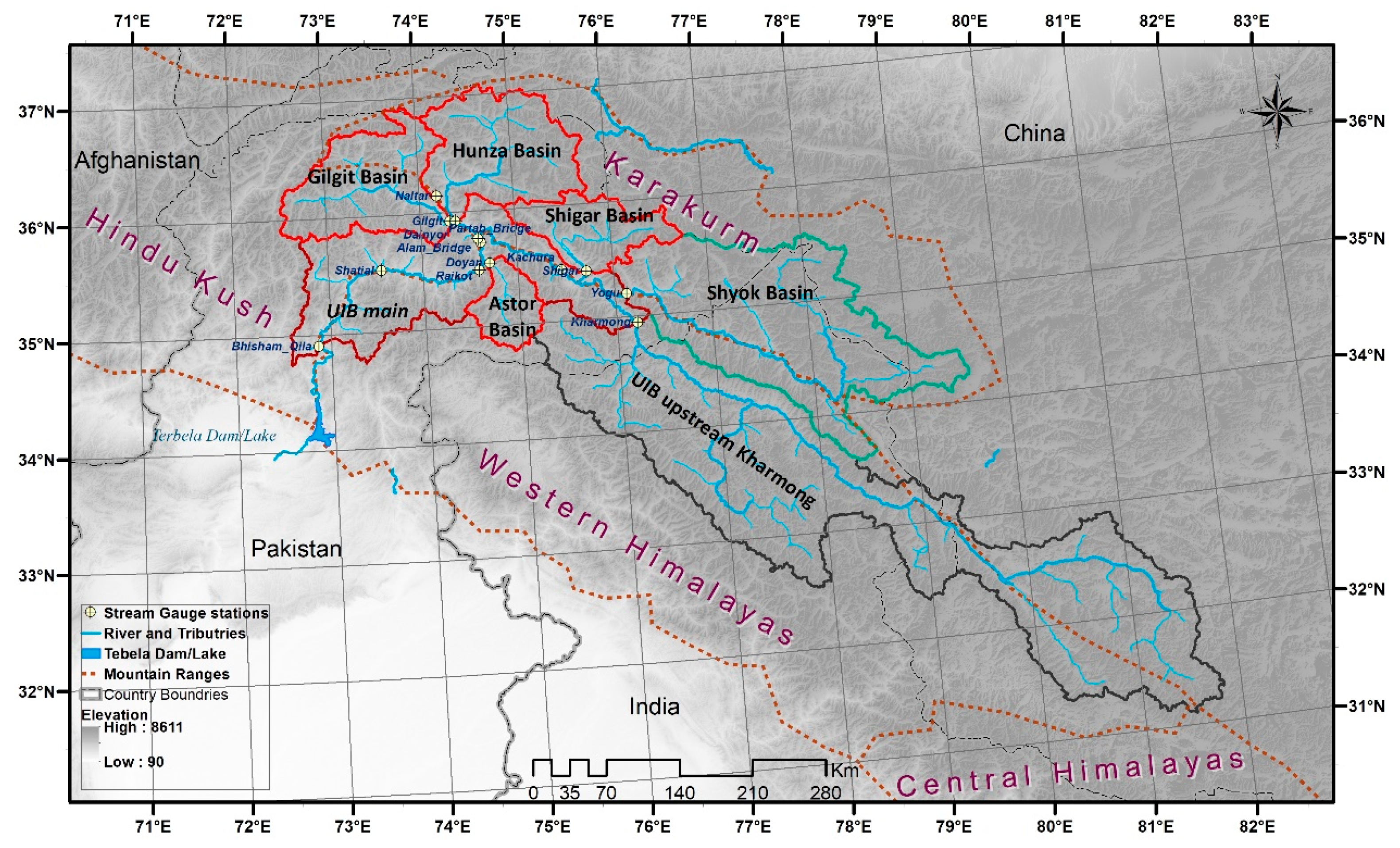
The Indus River, one of the largest rivers in Asia with a total length of about 2880 km, has a total drainage area of about 912,000 km2, which extends across portions of India, China, Pakistan and Afghanistan [13]. The section of the Indus upstream of the Tarbela Dam, Pakistan (Figure 1), which, according to our findings, has a length of about 1150 km and drains an area called the UIB, is approximately 165,400 km2.
Being a high mountain region, the UIB contains the largest area of perennial glacial ice cover of approximately 15,062 km2 outside the polar regions, with a volume of around 2174 km3 of the total ice reserves [35]. Some estimations [36] show even greater glacier cover, attaining an area of up to 12% of UIB (above 19,000 km2). The altitude of the UIB ranges from as low as 455 m to a maximum of 8611 m, and as a result, the climate varies greatly within the basin [10].
The summer monsoon has little effect on the basin, as almost 90% of its area is located in the rain shadow of the Himalayan belt [24]. Hence, except for the south-facing foothills, the intrusion of the Indian-ocean monsoon is limited by the mountains, so that its influence weakens northwestward [37]. Subsequently, the climatic controls in the UIB are quite different from that in the Himalayas on the eastern side. In fact, over the extent of the UIB, most of the annual precipitation originates from the mid-latitude western disturbances and mostly in solid form during winter and spring [25,38,39,40]. Occasional rains are brought in also by the monsoonal incursions into trans-Himalayan areas [38,40], but even during the summer months, the trans-Himalayan areas do not receive all precipitation from monsoon sources [41].
Climate variables are usually strongly influenced by topographic altitude. Thus, the northern valley floors of the UIB are arid, with an annual precipitation of only 100–200 mm which increases to 600 mm at a 4400-m altitude, and for higher elevations, glaciological studies suggest annual accumulation rates of 1500 to 2000 mm at 5500 m [40]. The average annual snow cover area in the UIB ranges from 10% to 70%, with its minimum in the summer snow melt period (June–September) and its maximum in the winter snow accumulation period (December–February) [10].
Stream flow in the UIB is generated by the combination of storm runoff in its lower part and snow and glacier runoff in its higher parts [12,13] Nearly half of the total annual flow in the whole Indus basin is contributed by the UIB, with a 86–88% contribution during the summer and only around 12–14% during the winter season [11,32].
2.2. Data Description
2.2.1. Reference Climate Data
The in situ meteorological observations in the UIB are sparse and mostly taken at (lower altitude) valley stations with very low spatial coverage. In addition, very little data is available for high altitudes. Furthermore, the orography of the UIB region is complex, leading to coactions of different hydro-climatic regimes which affect the amounts, spatial patterns and seasonality of the precipitation.
To cater for the non-representativeness and reported underestimations of the precipitation amounts by all the available data products [29,42], the current study has utilized a new corrected climate dataset generated by Khan and Koch [29,34].
This reference precipitation data set provided by Khan and Koch [29,34] is a combination of three sets of data: (1) 0.125° by 0.125° gridded precipitation time series for the 1997–2008 period, generated through the “informed-regionalization” methodology [29] which in turn is based on a relatively dense observing station network; (2) reconstructed precipitation time series for the time period of 1961–1995 for the parts of the UIB inside Pakistan’s borders (UIB-Pak) [34]; and (3) modified and corrected APHRODITE daily precipitation data available for the period 1961–2007 for parts of the UIB outside Pakistan’s borders [34].
The improvement and correction of the precipitation data has been done through a “Correction and Informed Regionalization (CIR)” approach. In the CIR methodology, the precipitation data is first quality checked and corrected for losses. Then, it is improved for a better spatial coverage through geospatial interpolation, followed by incorporation of a subbasin-specific “precipitation laps rate”, based on reported hydro-climatological data and the glacier mass balance dynamics in the UIB.
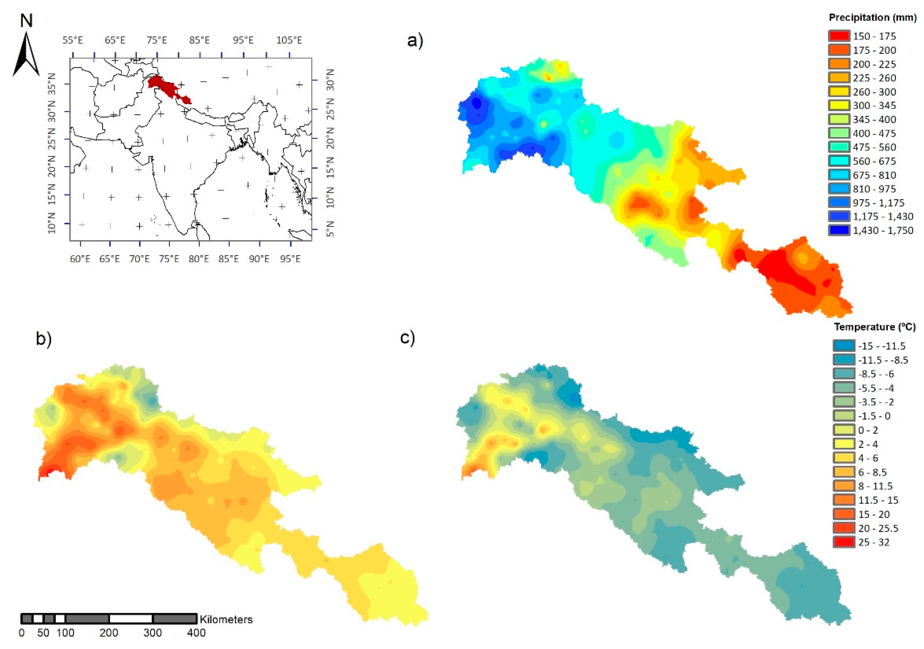
The temperature data used is acquired from Khan and Koch [34]. Similar to the precipitation dataset, the temperature data (1996 onwards) is also a combination of the spatially interpolated version of the available observed station data with adjustments by the region-specific, elevation-dependent lapse rate. Using the observed monthly time series variations, the temperature data was extrapolated to reconstruct missing data for the period 1961–1996 for the parts of UIB inside Pakistan’s border (UIB-Pak) and a modified and corrected version of APHRODITE data for the rest of the UIB outside Pakistan’s border. Figure 2 illustrates maps of precipitation and temperatures for the UIB. Full details of the methodology can be explored in References [29,34].
2.2.2. Reference Discharge Data
Daily river discharge data for a total of nine (9) hydrometric stations in the study area were collected from the Water & Power Development Authority, Lahore, Pakistan (WAPDA). These hydrometric stations are located on the main river (Indus) as well as its major tributaries (Table 1). It is important to note that, as the population and human intervention in the UIB is minimal, the flow regime is almost undisturbed and natural. As a matter of fact, central and eastern UIB, in particular, has in the past hardly seen any human-induced major influence on the rivers’ discharges; meanwhile, there are only minor single-season streamflow diversions for local irrigation, with minor effects in the western UIB [43,44]. There are, however, chances of interventions in the future as at least three major water reservoirs are proposed in the UIB, namely Bhasha dam, Dasu dam and Bunji dam. [45], which would have the capability to influence the flow regime in UIB. The current study has opted for future hydrological simulations without assessing the influences of the proposed dams as the exact timeline of their construction, inauguration or operation is not known.
2.2.3. Future Climate Forcing
The future climate forcing employed in the current study were adopted from Khan and Koch [17]. The data consisted of bias-corrected versions of five Coordinated Regional Climate Downscaling Experiment (CORDEX)-SA RCM experiments, namely IPSL-CM5A-MR_RCA4, MPI-ESM-LR_RCA4, NorESM1-M_RCA4, CanESM2_RegCM4-4 and iGFDL-ESM2M_RCA4. The downscaling for these five GCMs is done by CORDEX-SA, using two different RCMs (RCA4 and RegCM4). Their RCM outputs are at a considerably finer scale (0.44°) than those of the source GCMs.
This data was adopted as an effort to compensate for the uncertainties and variations between the different CMIP5 coupled climate models’ (GCM) results (or the regional climate model projections). Khan and Koch [17] recommended using a wider range of future climate scenarios for two representative concentration pathways (RCPs), namely RCP 4.5 and RCP 8.5, to force the SWAT hydrological model.
Khan and Koch [17] have carried the selection of possible future climate scenarios through a stepwise procedure, whereby future projections for RCP 4.5 and RCP 8.5 of the r1p1i1 ensemble from all climate models were screened based on three criteria: (1) the range of projected change in the mean, (2) range of projected change in the extremes and (3) skill in reproducing the past climate. The aim of this procedure was then to attain sets of four possible future extreme scenarios groups (wet-warm, wet-cold, dry-warm and dry-cold) for each RCP as well as of one scenario in each RCP group, representing the mean future climate change over the UIB. Using this category approach made it possible to arrive at a limited number of climate models. The final selection of a model was then carried out by assigning ranks based on the weighted score for each of the mentioned selection criteria. Khan and Koch [17] decided to utilize any dynamically downscaled version for the selected GCMs, ranked at the 1st or 2nd positions based on availability. As RCM projections were already available for the selected GCMs, five CORDEX-SA experiments (Table 2), including IPSL-CM5A-MR_RCA4, MPI-ESM-LR_RCA4, NorESM1-M_RCA4, Can ESM2_RegCM4-4 and GFDL-ESM2M_RCA4, were selected by Reference [17] for bias correction and further processing.
In the CORDEX-SA experiments, the downscaling for these five GCMs is done by using two different RCMs (RCA4 and RegCM4). Their RCM outputs are at a considerably finer scale (0.44°) than those of the source GCMs [17].
The five (5) selected (CORDEX-SA) RCM outputs have been further bias corrected using the “distribution mapping technique” [46] for RCP 4.5 and RCP 8.5 for two sets of durations, i.e., mid-century (2041–2070) and end-century (2071–2100).
The five (5) selected (CORDEX-SA) RCM outputs for RCP 4.5 and RCP 8.5 are bias corrected for two future periods, i.e., mid-century (2041–2070) and end-century (2071–2100) using the “distribution mapping technique”. Major properties of the downscaled projections are given in Table 3. Detailed descriptions of the downscaled and bias-corrected data can be found in Khan and Koch [17].
The downscaled projections by Khan and Koch [17] show changes/increases over all scenarios of temperature, ranging from 2.3 °C to 6.33 °C for RCP 4.5 and from 2.92 °C to as high as 9.0 °C for RCP 8.5. The higher temperature increase in this region may be attributed to the “elevation-dependent warming” phenomenon, whereby a larger temperature increase is expected in the mountains than in the neighboring plains and valleys of the UIB [16,21,22].
The changes in the downscaled and bias-corrected precipitation over the 21st century ranges from a minor increase of 2.2% for the drier scenarios to as high as 15.9% for the wet scenarios. Thus, both temperature and precipitation show increases, as do the extremes, since the probabilities of the wet days are projected to decrease while the precipitation intensities are projected to increase unanimously for both RCPs.
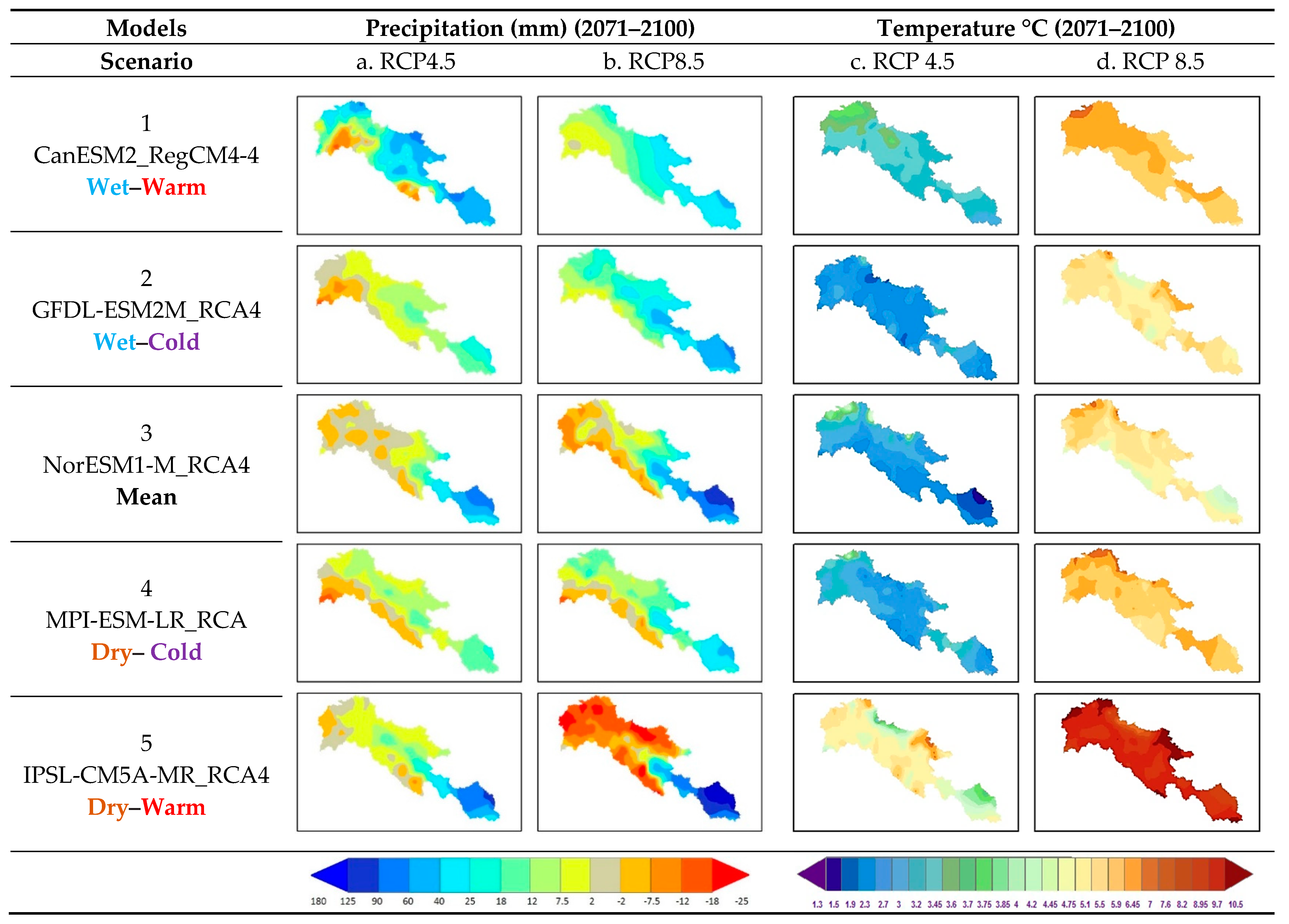
The spatial distribution of the projected changes in temperature and precipitation across the UIB also exhibits certain distinct trends (Figure 3). Thus, the late-century years (2071–2100) projected that precipitation changes show a decrease in the southeastern parts and an increase in the northeastern parts of the basin, and this holds for both RCPs. The spatial distributions of the projected changes in temperature show similarities for the two RCPs but with a higher increase in the northern and northwestern parts than in the eastern and southern part of the basin.
2.3. Hydrological Modelling
2.3.1. SWAT Model Description
The SWAT model is a continuous time (long-term yield) process-based semi-distributed hydrological model developed for the US Department of Agriculture (USDA), Agricultural Research Service (ARS), by Dr. Jeff Arnold [49]. It is capable of simulating long-term impacts of any management, climate or vegetation scenarios on the hydrological processes, pollution transport and sediment loading in river basins/watersheds [49,50]. In recent years, SWAT has been used more frequently, especially for the analysis of climate change hydrological impacts on stream flow and water yield [51,52,53].
To model the various physical/hydrological processes mentioned, SWAT requires specific information pertaining to the watershed such as weather, topography, soil properties, land cover, land use and management practices.
In the SWAT model, a river basin or watershed is partitioned into larger subunits called subbasins draining into the stream network and the river system. These subbasins are further divided into a series of smaller units, the hydrological response units (HRUs), which are nonspatial uniform units, each representing unique combinations of soil, land-use and slope. The calculations and simulations of hydrological components, sediment yield and nutrient cycles are first carried for each HRU and then aggregated for the subbasins and routed through the watershed.
The hydrological cycle simulated in SWAT is based on the water balance equation:
where and are respectively the initial and final soil water content (mm H2O) on day i, t is time (days), is the precipitation amount reaching the soil surface on day i (mm H2O), is the surface runoff amount on day i (mm H2O), is the evapotranspiration on day i (mm H2O), represents the interflow on day i (mm H2O) and is the return flow or base flow to the channel on day i (mm H2O).
The simulated hydrological components in SWAT include infiltration, redistribution, evapotranspiration (ET), lateral subsurface flow, groundwater or return flow, surface runoff, ponds inflow and outflow, transmission losses and water yield [49]. More detailed background and the theories of the SWAT-modelled hydrological process can be found in Reference [54].
2.3.2. Spatial Input Data and SWAT Model Setup
SWAT requires specific information pertaining to the watershed, such as topography, soil properties and land cover/land use, in addition to climate data and management practices in the basin.
The topographic data was provided in the form of a hydrologically conditioned digital elevation model (DEM), acquired from the “Hydrological data and maps based on SHuttle Elevation Derivatives at multiple Scales” (HydroSHEDS) website. This DEM has a resolution of 3 arc-seconds, is void-filled and is a hydrologically conditioned product [55], derived from the Shuttle Radar Topography Mission (SRTM) DEM [56].
The soil data were obtained from the FAO-UNESCO global soil map version 3.6 [57], which provides data for 5000 soil types comprising two layers (0–30 cm and 30–100 cm depth) at a spatial resolution of 5 km. For land use, the “Global Land Cover Characterization” (GLCC) at 1 km spatial resolution [58] was used.
The high-resolution DEM used in the study needed no preprocessing as it was already void-filled and hydrologically conditioned [55] and therefore provided almost no inconsistencies during the stream network delineation. For the watershed delineation process, “ArcSWAT-2012”, which is an ArcGIS-ArcView extension and graphical user input interface for the SWAT model, was used, choosing a threshold drainage area of 50,000 ha for the various subbasins. The whole watershed outlet as well as the monitoring gauge stations were manually added, while subbasin outlets were created by the software automatically based on the given threshold. As a result, the study area was finally configured with 173 subbasins, which were further divided into 2825 discrete HRUs based on the different soil and land-use classes, five (5) slope classes and ten (10) elevation bands. The total simulated watershed area in the current model is 165,611 km2.
2.3.3. Model Calibration and Validation Setup
The SWAT model was calibrated and validated against daily discharge data individually for each of its five (5) major tributaries (Hunza, Gilgit, Astor, Shigar and Shyok rivers), for parts of UIB (except the tributaries) inside Pakistan’s boundary and for UIB (situated in India China and Nepal) covering area upstream of Kharmong gauge station.
The Sequential Uncertainty Fitting SUFI-2 algorithm of the SWAT Calibration and Uncertainty Programs (SWAT-CUP) [59] was employed for parameter optimization. This algorithm is capable of mapping all uncertainties (parameter, inputs, conceptual model, etc.) in terms of parameter ranges as the procedure attempts to cover most of the measured data within the 95% prediction uncertainty (95PPU), which is calculated at the 2.5% and 97.5% levels of the cumulative distribution of all simulated output values. During this process, the user first assigns tangible ranges to a set of calibration parameters, where both (the ranges and the selection of calibration parameter) are guided by literature information, specific knowledge of the study area and the parameters’ sensitivity analysis. Once this is done, sets of samples (as many as intended simulations) are drawn from the parameter ranges through Latin hypercube sampling, followed by the SWAT model simulation using each of the sets and processed to evaluate various objective functions, as discussed below.
To quantify the goodness of model performance, i.e., the objective function, for the selected ranges of parameters in terms of calibration/uncertainty levels, two indices, the P-factor and the R-factor, are used. The P-factor denotes the percentage of data that is bracketed by the 95PPU band (ranging from 0 to 1, where 1 shows that all the predictions are within the 95PPU Band), while the R-factor is the average width of the 95PPU band divided by the standard deviation of the measured variable (0 to ∞, with 0 indicating a perfect match) [60,61,62].
For the evaluation of the calibration/validation results, the SUFI-2 algorithm allows the user to select from a range of different objective functions, such as the coefficient of determination (R2), percent bias (PBIAS), Nash–Sutcliffe efficiency (NS) or Kling-Gupta efficiency (KGE). The objective function can easily be reassigned in the post-processing step if required [59]. The current study used NS as the main objective function for the calibration/validation, but the results were also evaluated based on R2, PBIAS and KGE as well as the P-factor and the R-factor. Further details of the SWAT model calibration and validation setup are given in Appendices A–F (see Supplementary Materials, Appendices).
2.4. Assessment of Changes in Future Hydrology
The calibrated SWAT model was forced with the downscaled future climate projections for two RCPs (RCP 4.5 and RCP 8.5) of the five (5) selected CORDEX-SA climate models (see Section 2.2.3). For each scenario, the future hydrology is assessed for general flow characteristics, seasonality, high and low flows as well as extremes (return periods of extreme discharges) for two future periods, namely mid-century (2041–2070) and late-century (2071–2100).
These future hydrological assessments include calculations of percentage relative changes from the baseline period (1976–2005) for each of the hydrometeorological variables computed. These rates of change are calculated as follows:
where Xp and Xr denote the means of the hydrometeorological variable over the future projected and the reference periods, respectively.
The future changes in glacier/snowmelt contribution are estimated using the following modified hydrological balance equation proposed by Mark and Seltzer [63]:
Qt + P − E − Gw + Δg
According to which the total volume of water discharging from a catchment (per specified time period), Qt, is equal to the volume of water entering the catchment (Precipitation P) minus losses (i.e., evapotranspiration, E, and aquifer/groundwater recharge, Gw) plus changes in storage Δg in the system which comprise loss or gain of glacier ice volume, with snow/glacier accumulation (−) and snow/glacier melt contributions (+).
As the losses Gw may be minimal in comparison to the total discharge, especially for large mountainous catchments at an inter-annual time step, this term may be omitted in the equation above. Furthermore, by substituting Δg with the changes in snow/glacier accumulation/melt contributions (+ΔGm or −ΔGm), one gets the following:
In order to assess the future changes in the snow/glacier melt (ΔGm) contribution relative to that in the reference period, the above equation is rearranged as follows:
Similarly, future changes in the hydrological extremes are assessed in terms of the changes in the 1st and 99th percentiles of the flows, changes in the low and high flows, along with an analysis of the changes in recurrence intervals of extreme discharges, with return periods of 10, 15, and 30 years. These are calculated from a fitted Log-Pearson III value distribution to the simulated flow maxima for the reference and the two future 30-year periods: 1976–2005, 2041–2070 and 2071–2100, respectively.
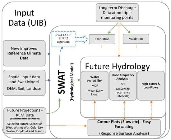
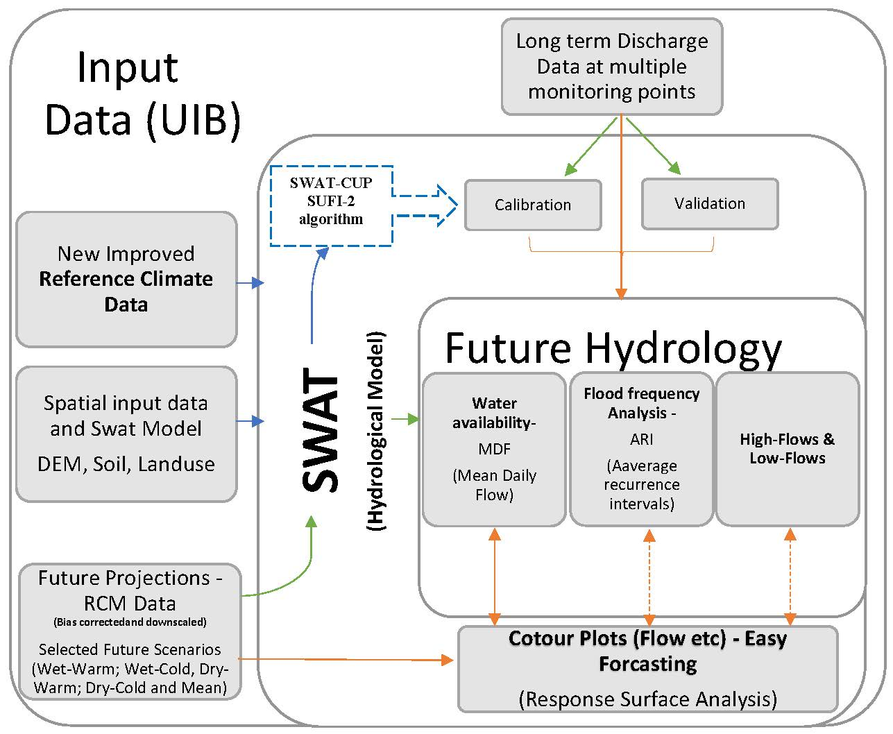
In addition to the above analysis, a 2nd order Response Surface Regression model (RSM) is applied to capture the interrelationship of mean annual “Flow” or “ET’ with mean annual precipitation and temperature for the projected future hydro-climatology. RSM models are multivariate polynomial models which utilize a set of mathematical equations to designate relationship between the response (e.g., flow) and the independent variables, e.g., temperature and precipitation [64]. Along with the fitted model, contour plots for the response variables “Flow” or “ET’ are also generated. The RSM, in addition to giving an overview of flow/evapotranspiration responses for different temperature and precipitation scenarios, is also usable for preliminary predictions of these hydrometeorological variables under diverse future precipitation and temperature changes. The calculations and plot generation have been done utilizing the “Response Surface Analysis” (RSA) program of the NCSS software (NCSS) (e.g., References [65,66]). A brief description of RSM is provided in Appendix H (see Supplementary Materials, Appendices).
3. Results and Discussion
3.1. Performance of the SWAT Model (Calibration-Validation)
For almost all tributaries included in the SWAT’s calibration process, the most sensitive calibration parameters turn out to be the ones related to snowmelt and groundwater and they are usually homogeneous across all the calibrated basins, i.e., there are only minor differences in the final best fitted ranges and values. A list of the calibrated parameters for the various tributary basins is provided in Appendix F (see Supplementary Materials, Appendices).
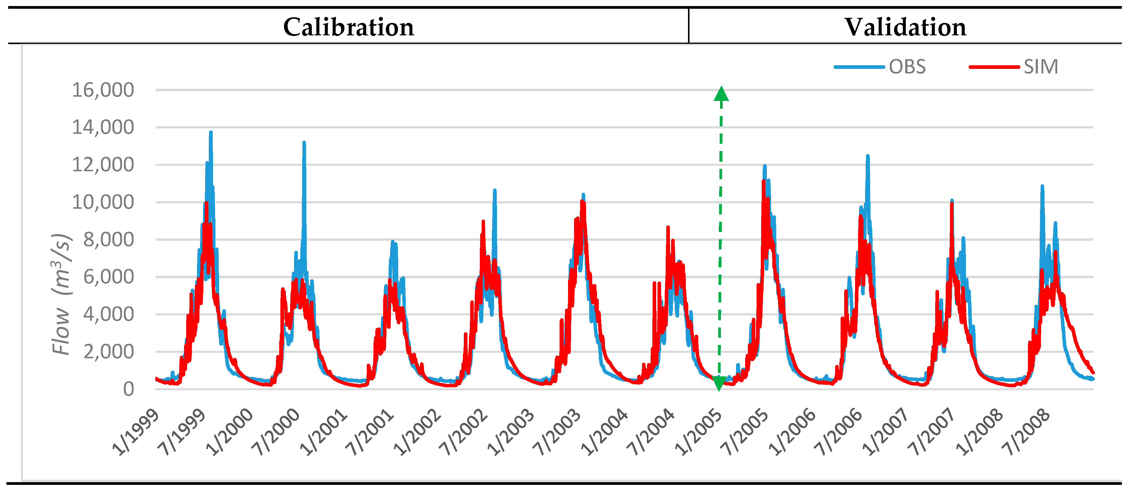
Results of the calibration and validation of the flow rates for the basin outlet at gauge station Bisham Qila are shown in Figure 4. One can notice that the SWA model is able not only to simulate most of the observed high and low flows at daily and monthly scales but also to capture the seasonal variation of the discharge as well. In fact, as listed in the figure and detailed in terms of the various performance statistical indicators (R2, NS coefficient, PBIAS and KGE) for all gauged stations at the tributaries outlets in Table 4, the calibrated SWAT simulations result in high NS, ranging from 0.69 to up to 0.86 for the flows at the tributaries’ outlets and between 0.70 and 0.89 at other monitoring points despite the fact that the UIB is a complex watershed to model, particularly on the daily time scale, as it covers a very vast area with a huge glaciated part and diverse hydro-climatic regimes as well as very sparse observation data. Table 4 indicates furthermore that, similar to the calibration period, the statistical results are also very good for the validation period.
3.2. Future Hydrology
3.2.1. Approach
The uncertainty in the UIB’s future climate is evidently also reflected in the SWAT simulated projections of the future hydrology. However, as will be shown in the following subsections, a number of consistent patterns in the projected changes in UIB’s future hydrology can be observed across the range of scenarios applied. To that avail, the calibrated SWAT model is forced with the downscaled future climate projections for the two RCPs (RCP 4.5 and RCP 8.5) of the five (5) selected CORDEX climate models (see Section 2.2.3). As listed in Table 2 earlier, each of the five (CORDEX-SA) RCMs selected represents essentially a particular future climate scenario, including the four possible future extreme scenarios groups (wet-warm, wet-cold, dry-warm dry-cold) for each RCP as well as of one scenario in each group, representing the mean future climate change over the UIB. For each scenario, the future hydrology is assessed for general flow characteristics, seasonality, high and low flows as well as extremes (return periods of extreme discharges) for two future periods, namely mid-century (2041–2070) and late-century (2071–2100). The results are summarized, along with other hydrometeorological variables and the glacier accumulation/melt (estimated with Equation (6)), both in absolute values and as relative changes compared with the historical reference period, in Table 5. The major features of this table are discussed in the subsequent subsections.
3.2.2. General Flow Characteristics
From Table 5, one can recognize that the projected changes in stream flow exhibit fairly consistent increases in the mid- as well as late-centuries for all future RCP/climate scenarios, except one, the dry-warm scenario (IPSL-MR-RCA4_RCP8.5 model), for which the simulation indicates a decrease in the mean daily flows (MDF) in both future periods. Apparently, in this dry-warm scenario, the increase in snow/glacier melt contributions to the flows (resulting from the obvious increase in temperature) is possibly balanced out and even surpassed by the decrease of snow accumulation (due to less snowfall owing to increased temperatures and, therefore, less snow melt) and increased losses from highly increased actual evapotranspiration (aET), which rises to 196 mm and 247 mm for the mid- and late-centuries, respectively, which for the latter represents more than a doubling from the aET value in the reference period. In fact, for this dry-warm scenario (IPSL_RCP 8.5_both periods), the possible increase in the simulated future flows owing to higher melting or precipitation seems to be overcompensated by as decrease owing to higher rates of aET (see shaded area in Table 5).
3.2.3. Response Surface Regression
The above findings regarding the relationships of both mean daily flow and aET with precipitation and temperature (Section 2.2.3) are explored further through “Response surface regression analysis/modelling (RSM)”. Contour plots of the two response surfaces for these two variables are illustrated in Figure 5 and Figure 6.
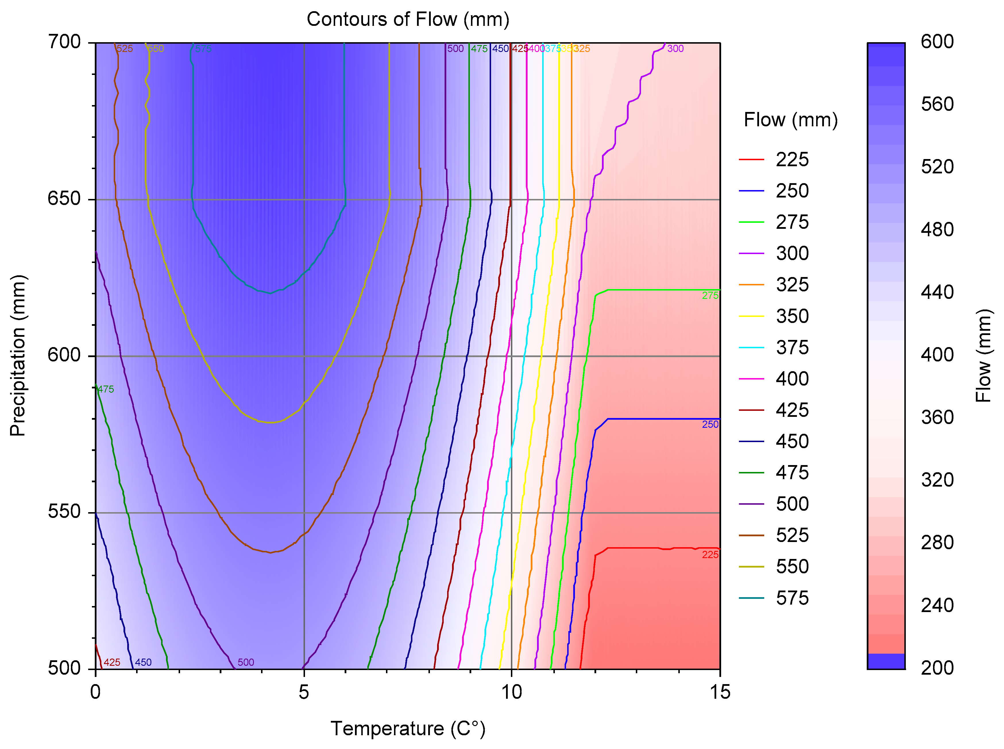
Regarding the “Flow” contour plot (Figure 5), its pattern is in line with the earlier discussed quantitative flow results for the UIB in response to different climatic scenarios, namely a steady flow increase with increasing future precipitation, as long as the future increase in temperature is less than 6 °C. This is a clear indication of the dominance of the snow accumulation and snow/glacier melting process over the influence of losses due to increased aET. However, when the projected temperature changes are above 5 °C to 6 °C, the losses due to increased aET become more dominant, so that the flow decreases almost linearly with increasing temperature, and this holds for any amount of mean annual precipitation.
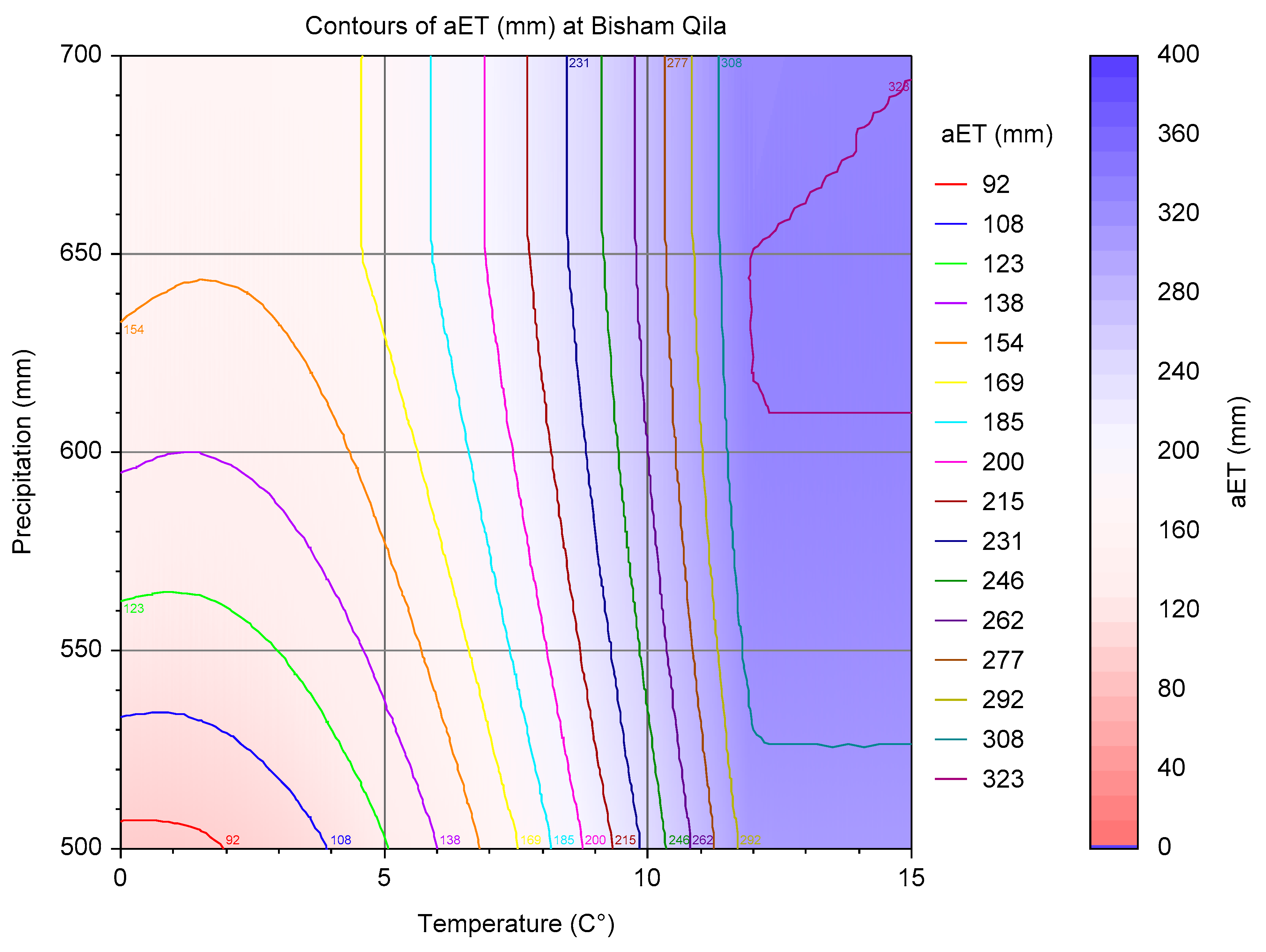
Similar behaviors are observable from the contour plot for “aET” (Figure 6) where, up to a projected temperature increase of 5° to 6 °C, the change in aET is mainly affected by precipitation, whereas for temperature changes beyond the 5 °C mark, aET increases with a gradient of ~30 mm/°C so that, at 10–12 °C, the aET rate saturates at values around 350 mm/year. Interestingly, the changes of aET in the temperature range 5 °C–10 °C and the precipitation range 550–650 mm/year are similar for 1 °C changes in temperature and 100 mm/year changes in precipitation. In other words, in the named temperature range, an increase of aET by increasing the temperature by 1 °C is largely offset if the precipitation increases by 100 mm/year.
In summary of this subsection, the generated contour maps of “Flow” (or “ET’) can also be used as an easy first guess or prediction of flow in the UIB under diverse future precipitation and temperature scenarios, especially when advanced modeling and forecasting is not feasible.
3.2.4. Monthly Flows and Seasonal Shifts
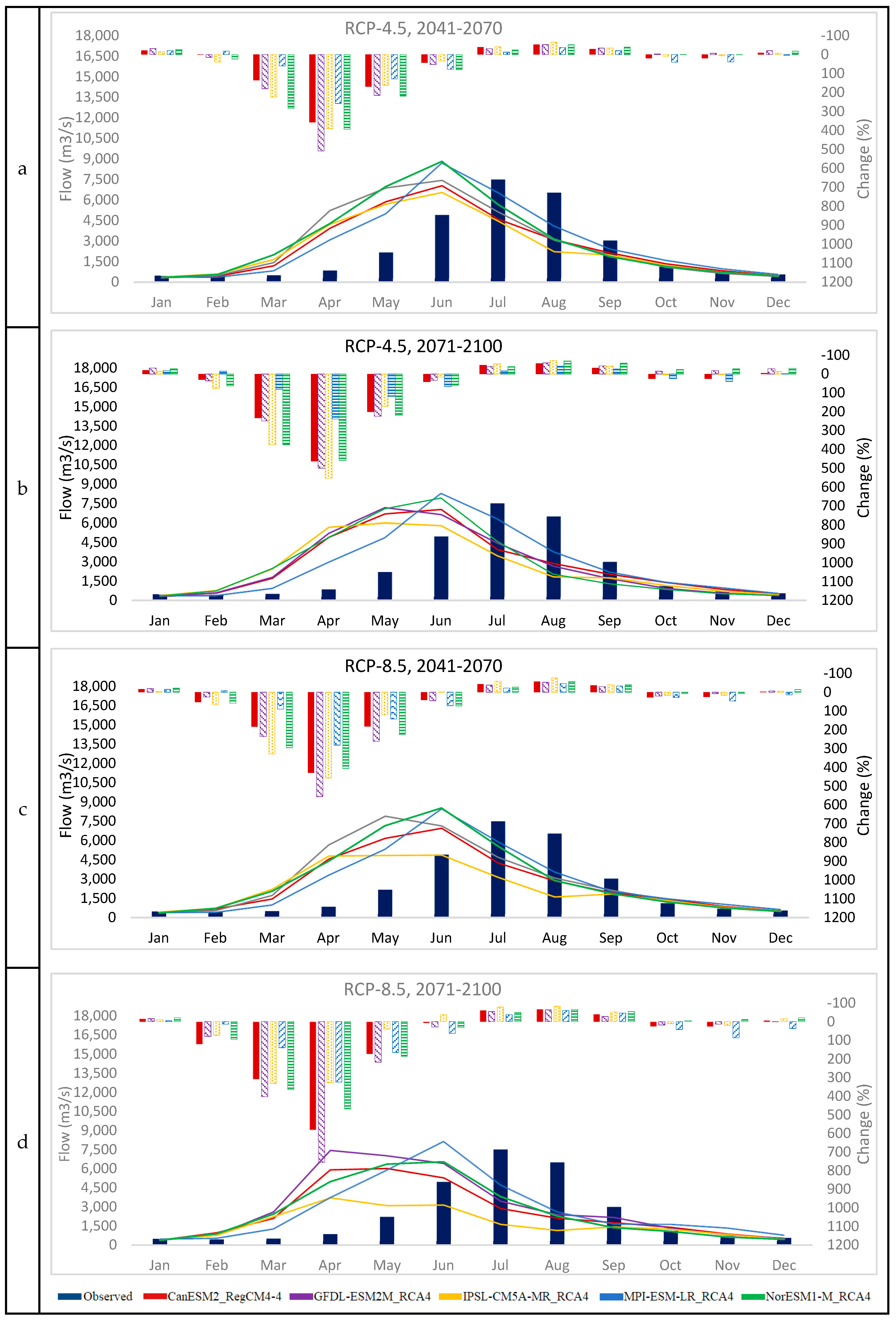
The UIB SWAT simulations show also changes in the future monthly and seasonal flows as indicated by the various panels of Figure 7. Thus, one may note changes in the yearly cycle and shifts in the timings of the high- and low-flow seasons, with similar trends but different magnitudes for the different scenarios.
For RCP 4.5 and all model/future period combinations considered, there is a shift of around one month in arrival of the peak flows, which is projected to be in June instead of July in the reference period. Simulations for RCP 8.5 show a similar trend, though with an even larger ahead-shift of up to two months. Also, for both RCPs and future periods, huge discharge increases are projected for the spring and early summer flows, so that the rise of the hydrograph in the future will start in spring rather than in midsummer, as for the reference period. The flow magnitudes in the spring season are also significantly higher than in the reference period (2 to 3 times for RCP 4.5 and 3–5 times for RCP 8.5). Furthermore, for all scenarios/periods, the future flow in autumn will be slightly increased. All these changes are most likely due to an increase in autumn or winter precipitation, leading to increased snow accumulation, and an earlier onset of snow/glacier-melt owing to rising temperatures.
For the RCP 8.5/late-century scenarios/periods, all five models project less increases and even a decrease for one model (IPSL) for the annual flows. The obvious reason is the higher rate of aET (Table 5), which negates the effect of increased precipitation and snow accumulation, so that for model IPSL which predicts less precipitation, the high aET induces considerable decreases in the average annual flows.
Our results above, for the intra-annual and magnitude changes of the flow, are in line with the projected hydrology of other studies (e.g., References [20,30,38]). Thus, a similar pattern of flows was reported by Lutz et al. [20] for RCP 8.5, namely, an earlier occurrence of higher-magnitude summer flows, particularly in the mid-century and less so towards the end of the 21st century.
3.3. Hydrological Extremes
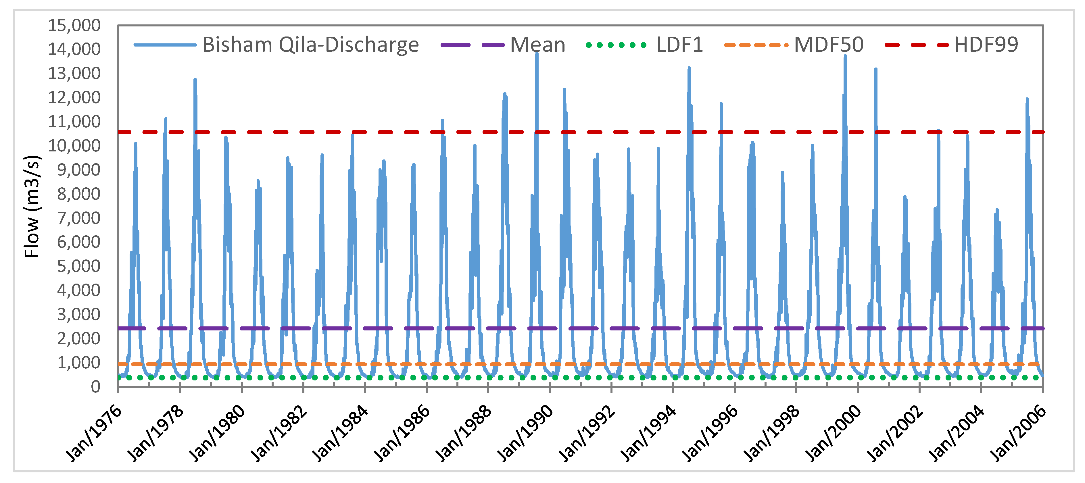
Future changes in the hydrological extremes, i.e., low and high flows, are evaluated through their exceedance levels for different return periods (return period flow) as well as in terms of the 1st and 99th percentiles of the flows as listed previously in Table 5. For a better appreciation of the subsequent statistical frequency analysis, the hydrograph of the daily observed discharge at the UIB outlet station Bisham Qila is shown for the reference period (1976–2005) in Figure 8, with the various flow quantiles drawn in as horizontal lines. Noticeable are the extreme peaks.
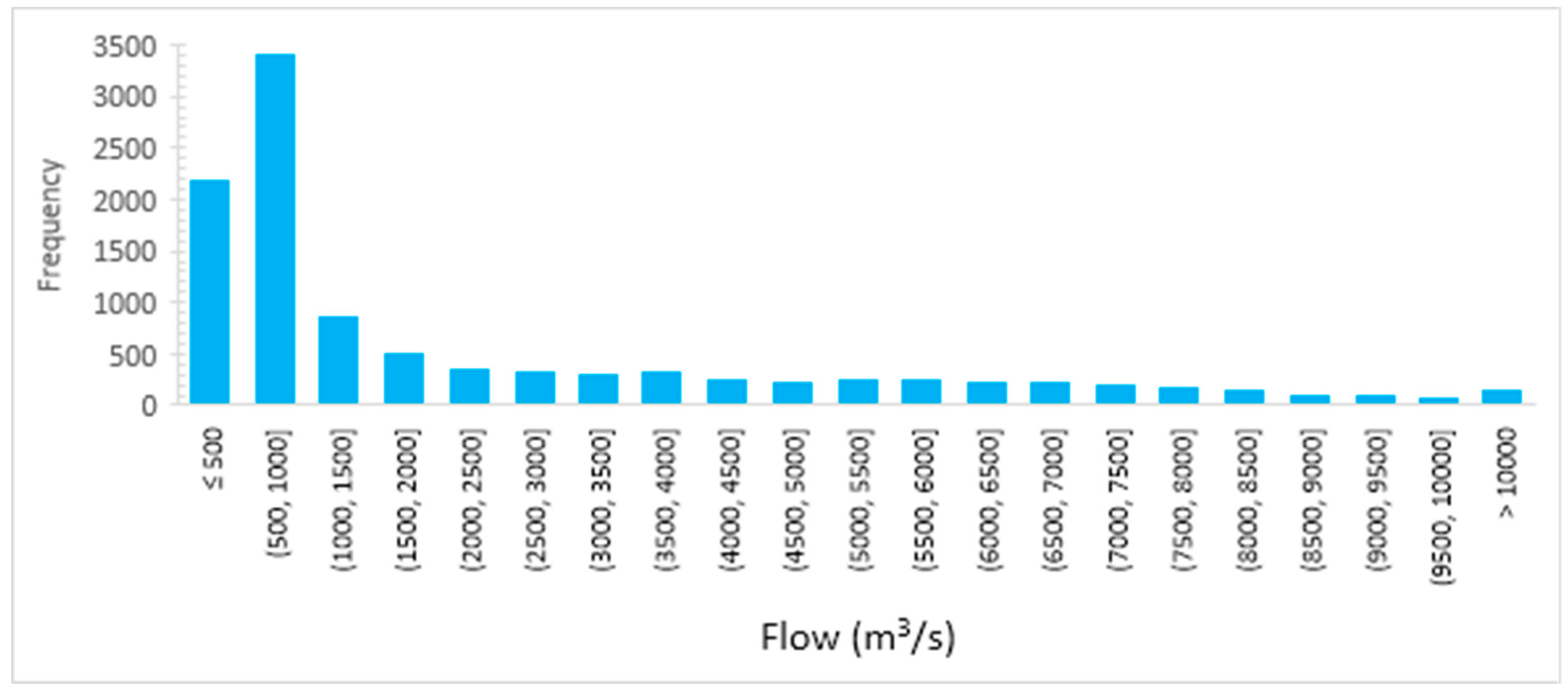
The frequency histogram of the daily discharge is shown in Figure 9, which hints of a strongly skewed extreme value distribution. A similar histogram behaviour is found for the annual maximum series used for the subsequent analysis of the return periods.
3.3.1. Annual Return Period Flows
For the evaluation of the annual return period (recurrence interval T) flow, exceedance probabilities (p = 1/T) of fitted Log-Pearson III value distributions (e.g., Reference [67]) to the observed (for the reference period) and the SWAT simulated future annual flow maxima using the various GCM Reg models’ climate projections for the different RCPs/future periods were computed.
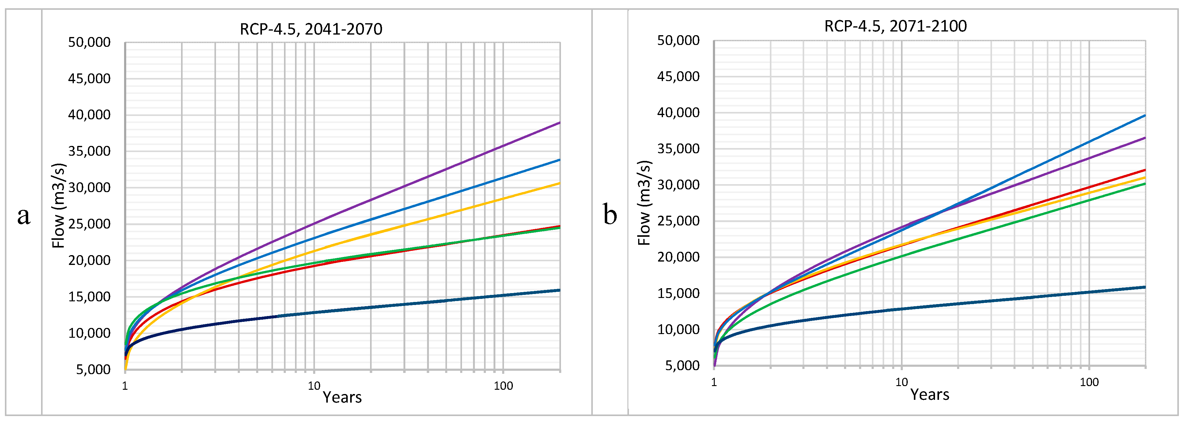
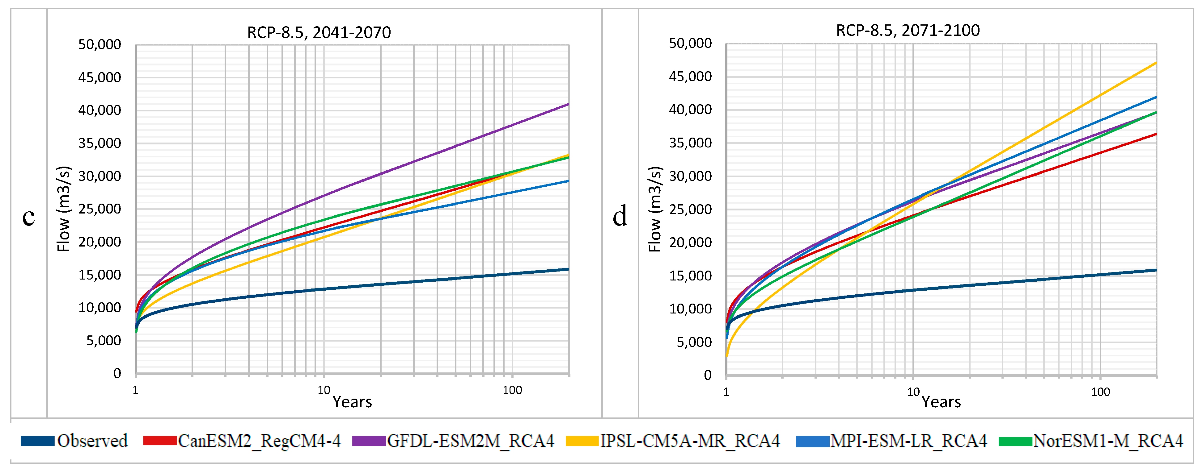
The four panels of Figure 10 show the annual return period flows obtained in this way, together with the ones for the reference period for the four RCP/future period combinations. Furthermore, the exceedance flows extracted for three return periods, i.e., 10, 15 and 30 years are listed in Table 6.
Both the figure and the table indicate remarkably more severe extreme discharges in the UIB compared to those in the reference period, in the mid-century and, depending on the model, often more so at the end of the century when exceedance flows are more than 100% higher than those in the reference period, particularly, for the more extreme RCP 8.5 scenario.
The different exceedance flow graphs in Figure 9 show similar patterns. Basically, for all tributaries and the main channel, the highest water discharge levels occur during the coinciding melting season (see Figure 7). Hence, the increases in the extreme return levels are essentially regulated by the projected climate/hydrology changes during those months and are due to the higher snow/glacier melt owing to the projected temperatures increase and higher accumulation of snow during the preceding winter and spring while coinciding with intense rainfall events which can considerably exacerbate the peak flows (see column LDF99 in Table 5).
Table 6 indicates more quantitatively that the projected future peak flow magnitudes will increase between 50% and above 100% for the three annual return intervals investigated (10, 15 and 30 years). Similarly, for the even longer return periods of 50, 100 and 200 years, the peak flood amounts will more than double, and this holds for all climate scenarios/periods/models (see Figure 10). In other words, what has been a 30-, 50-, 100- or even 200-year flood event in the past reference period will become a flood with a return period of 10 years or below, while a 10- or 20-year flood will be witnessed every 2 years in the future.
This imminent future situation is very alarming because, even under the current flow regime, there are catastrophic flood events every 10 to 20 years, with catastrophic human and economic consequences. Thus, the projected increase in flood frequencies means that the UIB and, especially, its downstream basin are likely to witness more frequent and more intense flood events unless appropriate flood protection measures are put into place. Other studies (e.g., Reference [20]) have reported similar future trends in the projected extreme flows.
3.3.2. High and Low Flows
For the analysis of various characteristics of the future low- and high-flow spells in the UIB, these spells have been defined here by the 1st (low daily flows (LDF1)) and 99th (high daily flows (DF99)) percentile historical flow discharges, as shown in Figure 8 and listed in Table 5, and which amount to threshold levels of 385 m3/s and 10,540 m3/s, respectively. In fact, the latter value corresponds roughly to a 2-year flood event for the reference period, as can be extracted from Figure 9.
The results of the SWAT simulations obtained with the various scenarios/periods/models are summarized in Table 7. From this table, one may notice similar future trends across all the assessed scenario combinations. More specifically, compared with the low-/high-flow values in the reference period (Table 7 and Figure 7), the magnitudes of mean low flow troughs at the 1st percentile have all decreased considerably (−13% to −19%), while the 99th percentile high flows all have significantly increased (10–25%) high spell peaks. Similarly, the magnitudes of the longest low flow spells for all the future scenarios have huge increases (21% to 132%), as do the magnitudes of the longest high flow spells, which have increased for all but the dry-warm scenario/model (RCP-8.5/IPSL-MR-RCA4), which predicts a huge future temperature increase but a precipitation decrease.
The results for the future high flow spells with discharges above the 99% threshold (10,540 m3/s) are in conformity with those of the previously computed projected return periods and flood magnitudes of floods (see Table 6), as the number of “high flow spells” have in most RCP/period/model cases increased by more than 300% in comparison to the reference period (Table 7). However, the mean duration of these future spells is considerably shorter by −15% to −69%, though some of them will also be much longer. All this means that these more frequent “high flow spell” events of shorter durations but with much higher peaks, i.e., flood concentration, will pose serious flood threats, as the present flood protection and retention infrastructures in the UIB are not designed for such extreme future floods.
In a similar manner, the 1% “low flow spells” (with troughs below 385 m3/s) are also projected to change drastically, as indicated by the appropriate columns of Table 7. Thus, the table shows that the UIB is expected to have more frequent and longer “low flow spell” events, especially for the wet-cold, dry-cold and mean model scenarios for both RCP/future periods. Although the wet-warm and dry-warm model scenarios will also have more frequent “low flow spell” events, these will have comparatively shorter durations than the others—possibly because of the high melt water contributions owing to the high future temperatures in these warm scenarios—but will still be much longer than those in the reference period.
4. Conclusions
Projecting future hydrology for the mountainous and highly glaciated UIB is a challenging task limited by many factors mainly due to uncertainties in the future climate projections and issues with the coverage and quality of available reference climatic data and hydrological modelling approaches. The current study has tried to investigate the impacts of future climate change on the hydrological behavior of the UIB during the 21st century while compensating for and avoiding, as much as possible, the limiting factors, so that the usability of the results could be enhanced as a viable set of future hydrological predictions.
The uncertainty in the future hydrological projections was addressed in two ways: (1) using reference data with improved quality, coverage and representation and (2) employing the wide range of different climate scenarios as provided by the various CORDEX GCM/RCM models in the SWAT model and getting diverse future hydrological projections. In addition, the full set of hydrological predictions was utilized to generate fitted Response Surface Regression Models (RSM) and contour maps for the two response variables “Mean Annual Flow” and “aET” as a function of the reference and projected mean annual precipitation and temperature. These RSMs can be used as a “hands-on” practical tool for preliminary forecast of the future hydrology in the UIB, under any temperature and precipitation projections, sourced from any climate model.
The overall results of the study are promising, since, notwithstanding the fact that there are always uncertainties in projecting future hydrological regime, almost all model/RCP scenarios have led to similar future trends of increased flows and intensified extremes. Thus, for all climate model scenarios under RCP 4.5, mean annual flows are projected to increase (relative to the 1976–2005 reference period) from 9.5–29.4% for the mid-century (2041–2070) period, while for the late century (2071–2100) period, a milder increase of only 10.2–19.1% is predicted. Similarly, all mean annual flow projections under RCP 8.5—except those based on model IPSL-MR-RCA4—show similar trends, with increases of 15.9–29.7% for the mid- and of only 9–27.5% for the late centuries. Here again, model IPSL-MR-RCA4 represents an exception, as its climate drivers lead to a steadily decreased SWAT simulated mean flow over the whole 21st century.
The seasonal shifts as well as the change in the extremes follow the same trends across all climate scenarios/models/period combinations analyzed. Hence, all projections show a future forward shift in the arrival of the peaks flows from, presently, July–August to late spring–early summer (May–June) as well as an increase of the magnitudes of the spring and winter flows.
The flow extremes are also projected to drastically intensify, with high (peak) floods having 50 to >100% more magnitude and tremendously decreased annual recurrence intervals, i.e., what has been something like a 100-year flood event or so in the past reference period will become a flood with a return period of 10 years or even below in the future. All this hint towards a tremendously increased flood hazard for the UIB in the future.
For the low flows, the more frequent and longer episodes with lower minimal flow values than those of the reference period are projected for all climate scenarios/models/period combinations, though these extreme alterations are somewhat milder for the future warm scenarios, most likely due to higher melt water contributions to the UIB flow discharge.
Supplementary Materials
The following are available online at https://0-www-mdpi-com.brum.beds.ac.uk/2071-1050/12/4/1283/s1, Appendices A–G: SWAT model setup, calibration and validation.
Author Contributions
Conceptualization, A.J.K.; formal analysis, A.J.K.; investigation, A.J.K.; methodology, A.J.K.; resources, M.K. and A.A.T.; supervision, M.K.; validation, A.J.K.; writing—original draft, A.J.K.; writing—review and editing, M.K. and A.A.T. All authors have read and agreed to the published version of the manuscript.
Funding
This research received no external funding.
Acknowledgments
We acknowledge provision of data by the following sources: Hydro-Shed-3sec GRID: Conditioned DEM, courtesy of the U.S. Geological Survey; FAO-UNESCO Soil Map of the World, version 3.6, courtesy of the Food and Agriculture Organization of the United Nations, FAO GEONETWORK, 2007; GLCC—Global Land Cover Characteristics Data Base, Version 2.0, courtesy of the U.S. Geological Survey, USGS EROS Data Centre; and Water and Power Development Authority (WAPDA) and Pakistan Meteorological Department (PMD) for their exchange of the valuable hydrological and climate data to complete my research.
Conflicts of Interest
The authors declare no conflict of interest.
References
- Qin, D.; Chen, Z.; Averyt, K.B.; Miller, H.L.; Solomon, S.; Manning, M.; Marquis, M.; Tignor, M. IPCC, 2013: Summary for Policymakers. In Climate Change 2013: The Physical Science Basis. Contribution of Working Group I to the Fifth Assessment Report of the Intergovernmental Panel on Climate Change; Stocker, T.F., Qin, D., Plattner, G.-K., Tignor, M., Allen, S.K., Boschung, J., Nauels, A., Xia, Y., Bex, V., Midgley, P.M., Eds.; Cambridge University Press: Cambridge, UK; New York, NY, USA, 2013. [Google Scholar]
- Milly, P.C.D.; Dunne, K.A.; Vecchia, A.V. Global pattern of trends in streamflow and water availability in a changing climate. Nature 2005, 438, 347–350. [Google Scholar] [CrossRef] [PubMed]
- Kim, S.; Tachikawa, Y.; Nakakita, E.; Yorozu, K.; Shiiba, M. Climate change impact on river flow of the tone river basin, Japan. J. Jpn. Soc. Civ. Eng. Ser. B1 Hydraul. Eng. 2011, 67, I_85–I_90. [Google Scholar] [CrossRef] [Green Version]
- Oki, T.; Kanae, S. Global hydrological cycles and world water resources. Science 2006, 313, 1068–1072. [Google Scholar] [CrossRef] [PubMed] [Green Version]
- Abbaspour, K.C.; Faramarzi, M.; Ghasemi, S.S.; Yang, H. Assessing the impact of climate change on water resources in Iran. Water Resour. Res. 2009, 45, 413. [Google Scholar] [CrossRef] [Green Version]
- Fowler, H.J.; Kilsby, C.G.; O’Connell, P.E. Modeling the impacts of climatic change and variability on the reliability, resilience, and vulnerability of a water resource system. Water Resour. Res. 2003, 39, 39. [Google Scholar] [CrossRef] [Green Version]
- Kilroy, G. A review of the biophysical impacts of climate change in three hotspot regions in Africa and Asia. Reg. Environ. Chang. 2015, 15, 771–782. [Google Scholar] [CrossRef] [Green Version]
- Hussain, M.; Mumtaz, S. Climate change and managing water crisis: Pakistan’s perspective. Rev. Environ. Health 2014, 29, 71–77. [Google Scholar] [CrossRef]
- Hassan, Z.; Shabbir, R.; Ahmad, S.S.; Malik, A.H.; Aziz, N.; Butt, A.; Erum, S. Dynamics of land use and land cover change (LULCC) using geospatial techniques: A case study of Islamabad Pakistan. Springerplus 2016, 5, 812. [Google Scholar] [CrossRef] [Green Version]
- Khan, F.; Pilz, J.; Amjad, M.; Wiberg, D.A. Climate variability and its impacts on water resources in the Upper Indus Basin under IPCC climate change scenarios. Int. J. Glob. Warm. 2015, 8, 46. [Google Scholar] [CrossRef]
- Tahir, A.A.; Chevallier, P.; Arnaud, Y.; Ahmad, B. Snow cover dynamics and hydrological regime of the Hunza River basin, Karakoram Range, Northern Pakistan. Hydrol. Earth Syst. Sci. 2011, 15, 2275–2290. [Google Scholar] [CrossRef] [Green Version]
- Archer, D. Contrasting hydrological regimes in the upper Indus Basin. J. Hydrol. 2003, 274, 198–210. [Google Scholar] [CrossRef]
- Ali, K.F.; de Boer, D.H. Spatial patterns and variation of suspended sediment yield in the upper Indus River basin, northern Pakistan. J. Hydrol. 2007, 334, 368–387. [Google Scholar] [CrossRef]
- Immerzeel, W.W.; van Beek, L.P.H.; Bierkens, M.F.P. Climate change will affect the Asian water towers. Science 2010, 328, 1382–1385. [Google Scholar] [CrossRef] [PubMed]
- Lutz, A.F.; Immerzeel, W.W.; Kraaijenbrink, P.D.A.; Shrestha, A.B.; Bierkens, M.F.P. Climate Change Impacts on the Upper Indus Hydrology: Sources, Shifts and Extremes. PLoS ONE 2016, 11, e0165630. [Google Scholar] [CrossRef] [PubMed] [Green Version]
- Wijngaard, R.R.; Lutz, A.F.; Nepal, S.; Khanal, S.; Pradhananga, S.; Shrestha, A.B.; Immerzeel, W.W. Future changes in hydro-climatic extremes in the Upper Indus, Ganges, and Brahmaputra River basins. PLoS ONE 2017, 12, e0190224. [Google Scholar] [CrossRef] [PubMed]
- Khan, A.; Koch, M. Selecting and Downscaling a Set of Climate Models for Projecting Climatic Change for Impact Assessment in the Upper Indus Basin (UIB). Climate 2018, 6, 89. [Google Scholar] [CrossRef] [Green Version]
- Rajbhandari, R.; Shrestha, A.B.; Kulkarni, A.; Patwardhan, S.K.; Bajracharya, S.R. Projected changes in climate over the Indus river basin using a high resolution regional climate model (PRECIS). Clim. Dyn. 2015, 44, 339–357. [Google Scholar] [CrossRef] [Green Version]
- Forsythe, N.; Fowler, H.J.; Blenkinsop, S.; Burton, A.; Kilsby, C.G.; Archer, D.R.; Harpham, C.; Hashmi, M.Z. Application of a stochastic weather generator to assess climate change impacts in a semi-arid climate: The Upper Indus Basin. J. Hydrol. 2014, 517, 1019–1034. [Google Scholar] [CrossRef] [Green Version]
- Laghari, A.N.; Vanham, D.; Rauch, W. The Indus basin in the framework of current and future water resources management. Hydrol. Earth Syst. Sci. 2012, 16, 1063–1083. [Google Scholar] [CrossRef] [Green Version]
- Palazzi, E.; Filippi, L.; von Hardenberg, J. Insights into elevation-dependent warming in the Tibetan Plateau-Himalayas from CMIP5 model simulations. Clim. Dyn. 2017, 48, 3991–4008. [Google Scholar] [CrossRef] [Green Version]
- Pepin, N.; Bradley, R.S.; Diaz, H.F.; Baraer, M.; Caceres, E.B.; Forsythe, N.; Fowler, H.; Greenwood, G.; Hashmi, M.Z.; Liu, X.D.; et al. Elevation-dependent warming in mountain regions of the world. Nat. Clim. Chang. 2015, 5, 424–430. [Google Scholar] [CrossRef] [Green Version]
- Khan, S.I.; Adams, T.E. Introduction of Indus River Basin: Water Security and Sustainability. In Indus River Basin, 1st ed.; Khan, S.I., Ed.; Elsevier: Cambridge, MA, USA, 2019; pp. 3–16. ISBN 9780128127827. [Google Scholar]
- Immerzeel, W.W.; Droogers, P.; de Jong, S.M.; Bierkens, M.F.P. Large-scale monitoring of snow cover and runoff simulation in Himalayan river basins using remote sensing. Remote Sens. Environ. 2009, 113, 40–49. [Google Scholar] [CrossRef]
- ul Hasson, S. Future Water Availability from Hindukush-Karakoram-Himalaya upper Indus Basin under Conflicting Climate Change Scenarios. Climate 2016, 4, 40. [Google Scholar] [CrossRef] [Green Version]
- Bocchiola, D.; Diolaiuti, G.; Soncini, A.; Mihalcea, C.; D’Agata, C.; Mayer, C.; Lambrecht, A.; Rosso, R.; Smiraglia, C. Prediction of future hydrological regimes in poorly gauged high altitude basins: The case study of the upper Indus, Pakistan. Hydrol. Earth Syst. Sci. 2011, 15, 2059–2075. [Google Scholar] [CrossRef] [Green Version]
- Palazzi, E.; von Hardenberg, J.; Provenzale, A. Precipitation in the Hindu-Kush Karakoram Himalaya: Observations and future scenarios. J. Geophys. Res. Atmos. 2013, 118, 85–100. [Google Scholar] [CrossRef]
- Yatagai, A.; Kamiguchi, K.; Arakawa, O.; Hamada, A.; Yasutomi, N.; Kitoh, A. APHRODITE: Constructing a Long-Term Daily Gridded Precipitation Dataset for Asia Based on a Dense Network of Rain Gauges. Bull. Am. Meteorol. Soc. 2012, 93, 1401–1415. [Google Scholar] [CrossRef]
- Khan, A.; Koch, M. Correction and Informed Regionalization of Precipitation Data in a High Mountainous Region (Upper Indus Basin) and Its Effect on SWAT-Modelled Discharge. Water 2018, 10, 1557. [Google Scholar] [CrossRef] [Green Version]
- Soncini, A.; Bocchiola, D.; Confortola, G.; Bianchi, A.; Rosso, R.; Mayer, C.; Lambrecht, A.; Palazzi, E.; Smiraglia, C.; Diolaiuti, G. Future Hydrological Regimes in the Upper Indus Basin: A Case Study from a High-Altitude Glacierized Catchment. J. Hydrometeorol. 2015, 16, 306–326. [Google Scholar] [CrossRef] [Green Version]
- Akhtar, M.; Ahmad, N.; Booij, M.J. The impact of climate change on the water resources of Hindukush–Karakorum–Himalaya region under different glacier coverage scenarios. J. Hydrol. 2008, 355, 148–163. [Google Scholar] [CrossRef]
- Khan, F.; Pilz, J.; Ali, S. Improved hydrological projections and reservoir management in the Upper Indus Basin under the changing climate. Water Environ. J. 2017, 31, 235–244. [Google Scholar] [CrossRef]
- Immerzeel, W.W.; Pellicciotti, F.; Bierkens, M.F.P. Rising river flows throughout the twenty-first century in two Himalayan glacierized watersheds. Nat. Geosci. 2013, 6, 742–745. [Google Scholar] [CrossRef]
- Khan, A.J.; Koch, M. Long-Term daily gridded precipitation dataset for Upper Indus Basin (UIB) through Temporal reconstruction, Correction and informed regionalization-“ReCIR-PCP”. Water. under review.
- Bajracharya, S.R.; Shrestha, B. (Eds.) The Status of Glaciers in the Hindu Kush-Himalayan Region; International Centre for Integrated Mountain Development: Kathmandu, Nepal, 2011; ISBN 9789291152179. [Google Scholar]
- RGI Consortium. Randolph Glacier Inventory—A Dataset of Global Glacier Outlines: Version 5.0: Technical Report, Global Land Ice Measurements from Space, Version 5.0; Digital Media: Denver, CO, USA, 2015. [Google Scholar]
- Bookhagen, B.; Burbank, D.W. Topography, relief, and TRMM-derived rainfall variations along the Himalaya. Geophys. Res. Lett. 2006, 33, 21. [Google Scholar] [CrossRef] [Green Version]
- Ali, S.; Li, D.; Congbin, F.; Khan, F. Twenty first century climatic and hydrological changes over Upper Indus Basin of Himalayan region of Pakistan. Environ. Res. Lett. 2015, 10, 14007. [Google Scholar] [CrossRef]
- Hewitt, K. Glacier Change, Concentration, and Elevation Effects in the Karakoram Himalaya, Upper Indus Basin. Mt. Res. Dev. 2011, 31, 188–200. [Google Scholar] [CrossRef]
- Wake, C.P. Glaciochemical Investigations as a Tool for Determining the Spatial and Seasonal Variation of Snow Accumulation in the Central Karakoram, Northern Pakistan. Ann. Glaciol. 1989, 13, 279–284. [Google Scholar] [CrossRef] [Green Version]
- Karim, A.; Veizer, J. Water balance of the Indus River Basin and moisture source in the Karakoram and western Himalayas: Implications from hydrogen and oxygen isotopes in river water. J. Geophys. Res. 2002, 107, 190. [Google Scholar] [CrossRef]
- Khan, A.; Koch, M.; Chinchilla, K. Evaluation of Gridded Multi-Satellite Precipitation Estimation (TRMM-3B42-V7) Performance in the Upper Indus Basin (UIB). Climate 2018, 6, 76. [Google Scholar] [CrossRef] [Green Version]
- Hasson, S.; Böhner, J.; Lucarini, V. Prevailing climatic trends and runoff response from Hindukush–Karakoram–Himalaya, upper Indus Basin. Earth Syst. Dyn. 2017, 8, 337–355. [Google Scholar] [CrossRef] [Green Version]
- Khattak, M.S.; Babel, M.S.; Sharif, M. Hydro-meteorological trends in the upper Indus River basin in Pakistan. Clim. Res. 2011, 46, 103–119. [Google Scholar] [CrossRef]
- Amin, A.; Iqbal, J.; Asghar, A.; Ribbe, L. Analysis of Current and Future Water Demands in the Upper Indus Basin under IPCC Climate and Socio-Economic Scenarios Using a Hydro-Economic WEAP Model. Water 2018, 10, 537. [Google Scholar] [CrossRef] [Green Version]
- Teutschbein, C.; Seibert, J. Bias correction of regional climate model simulations for hydrological climate-change impact studies: Review and evaluation of different methods. J. Hydrol. 2012, 456, 12–29. [Google Scholar] [CrossRef]
- Giorgi, F.; Coppola, E.; Solmon, F.; Mariotti, L.; Sylla, M.B.; Bi, X.; Elguindi, N.; Diro, G.T.; Nair, V.; Giuliani, G.; et al. RegCM4: Model description and preliminary tests over multiple CORDEX domains. Clim. Res. 2012, 52, 7–29. [Google Scholar] [CrossRef] [Green Version]
- Samuelsson, P.; Jones, C.G.; Will’En, U.; Ullerstig, A.; Gollvik, S.; Hansson, U.; Jansson, E.; Kjellstro¨M, C.; Nikulin, G.; Wyser, K. The Rossby Centre Regional Climate model RCA3: Model description and performance. Tellus A Dyn. Meteorol. Oceanogr. 2011, 63, 4–23. [Google Scholar] [CrossRef] [Green Version]
- Arnold, J.G.; Srinivasan, R.; Muttiah, R.S.; Williams, J.R. Large area hydrologic modeling and assessment part i: Model development. J. Am. Water Resour. Assoc. 1998, 34, 73–89. [Google Scholar] [CrossRef]
- Srinivasan, R.; Ramanarayanan, T.S.; Arnold, J.G.; Bednarz, S.T. Large area hydrologic modeling and assessment part ii: Model application. J. Am. Water Resour. Assoc. 1998, 34, 91–101. [Google Scholar] [CrossRef]
- Cherie, N.; Koch, M. (Eds.) Mono- and multi-Model statistical Downscaling of GCM—Climate Predictors for the Upper Blue Nile River Basin, Ethiopia. In Proceedings of the 6th International Conference on Water Resources and Enviromental Research (ICWRER), Koblenz, Germany, 3–7 June 2013. [Google Scholar]
- Fereidoon, M.; Koch, M. SWAT-MODSIM-PSO optimization of multi-crop planning in the Karkheh River Basin, Iran, under the impacts of climate change. Sci. Total Environ. 2018, 630, 502–516. [Google Scholar] [CrossRef]
- Kundu, S.; Khare, D.; Mondal, A. Individual and combined impacts of future climate and land use changes on the water balance. Ecol. Eng. 2017, 105, 42–57. [Google Scholar] [CrossRef]
- Neitsch, S.L.; Arnold, J.G.; Kiniry, J.R.; Williams, J.R. Soil and Water Assessment Tool, Theoretical Documentation, Version 2009; Texas Water Resources Institute Technical Report No. 406. Available online: https://swat.tamu.edu/media/99192/swat2009-theory.pdf (accessed on 9 February 2020).
- Lehner, B.; Verdin, K.; Jarvis, A. New Global Hydrography Derived From Spaceborne Elevation Data. Eos Trans. Am. Geophys. Union 2008, 89, 93–94. [Google Scholar] [CrossRef]
- Farr, T.G.; Rosen, P.A.; Caro, E.; Crippen, R.; Duren, R.; Hensley, S.; Kobrick, M.; Paller, M.; Rodriguez, E.; Roth, L.; et al. The Shuttle Radar Topography Mission. Rev. Geophys. 2007, 45, 1485. [Google Scholar] [CrossRef] [Green Version]
- FAO-UNESCO. FAO-UNESCO Soil Map of the World, Version 3.6; Food and Agriculture Organization of the United Nations. FAO GEONETWORK: Rome, Italy, 2007. [Google Scholar]
- USGS EROS Data Center. GLCC—Global Land Cover Characteristics Data Base, Version 2.0; USGS, Earth Resources Observation and Science (EROS) Center: Garretson, SD, USA, 2002.
- Abbaspour, K.C. SWAT Calibration and Uncertainty Program—A User Manual; Swiss Federal Institute of Aquatic Science and Technology: Eawag, Switzerland, 2015. [Google Scholar]
- Abbaspour, K.C.; Yang, J.; Maximov, I.; Siber, R.; Bogner, K.; Mieleitner, J.; Zobrist, J.; Srinivasan, R. Modelling hydrology and water quality in the pre-alpine/alpine Thur watershed using SWAT. J. Hydrol. 2007, 333, 413–430. [Google Scholar] [CrossRef]
- Schuol, J.; Abbaspour, K.C.; Srinivasan, R.; Yang, H. Estimation of freshwater availability in the West African sub-continent using the SWAT hydrologic model. J. Hydrol. 2008, 352, 30–49. [Google Scholar] [CrossRef]
- Yang, J.; Reichert, P.; Abbaspour, K.C.; Xia, J.; Yang, H. Comparing uncertainty analysis techniques for a SWAT application to the Chaohe Basin in China. J. Hydrol. 2008, 358, 1–23. [Google Scholar] [CrossRef]
- Mark, B.G.; Seltzer, G.O. Tropical glacier meltwater contribution to stream discharge: A case study in the Cordillera Blanca, Peru. J. Glaciol. 2003, 49, 271–281. [Google Scholar] [CrossRef] [Green Version]
- Yu, J.; Qin, X.; Larsen, O.; Chua, L.H.C. Comparison between Response Surface Models and Artificial Neural Networks in Hydrologic Forecasting. J. Hydrol. Eng. 2014, 19, 473–481. [Google Scholar] [CrossRef]
- Carley, K.M.; Kamneva, N.Y.; Reminga, J. Response Surface Methodology: CASOS Technical Report; Carnegie Mellon University, Institute for Software Research International: Pittsburgh, PA, USA, 2004; CMU-ISR-04-136. [Google Scholar]
- Keshtegar, B.; Allawi, M.F.; Afan, H.A.; El-Shafie, A. Optimized River Stream-Flow Forecasting Model Utilizing High-Order Response Surface Method. Water Resour. Manag. 2016, 30, 3899–3914. [Google Scholar] [CrossRef]
- Chow, V.T.; Maidment, D.R.; Mays, L.W. Applied Hydrology; Tata McGraw-Hill, Ed.; Tata McGraw-Hill Education: New Delhi, NY, USA, 2010; ISBN 007070242X. [Google Scholar]
Figure 1.
Upper Indus Basin (UIB) extent, tributary catchments, major streams, stream gauge stations and elevation details.
Figure 1.
Upper Indus Basin (UIB) extent, tributary catchments, major streams, stream gauge stations and elevation details.

Figure 2.
Reference climate data: (a) mean annual precipitation (mm); (b) mean temperature, maximum (°C); and (c) mean temperature, minimum (°C).
Figure 2.
Reference climate data: (a) mean annual precipitation (mm); (b) mean temperature, maximum (°C); and (c) mean temperature, minimum (°C).

Figure 3.
UIB-projected changes in precipitation and temperature over the late-century (2071-2100) obtained with the 5 CORDEX-model experiments (see Table 2) under 2 RCPs.
Figure 3.
UIB-projected changes in precipitation and temperature over the late-century (2071-2100) obtained with the 5 CORDEX-model experiments (see Table 2) under 2 RCPs.

Figure 4.
The Soil and Water Assessment Tool (SWAT) simulated and observed UIB flows at Bisham Qila during calibration and validation periods (goodness-of-fit statistics between observed and simulated values presented include Nash–Sutcliffe efficiency (NSE), Coefficient of Determination (R2), Percent Bias (pbias) and Kling–Gupta efficiency (KGE).

Figure 5.
Contour plot of UIB mean annual (out) flow at gauge station Bisham Qila for a range of future-predicted temperature and precipitation scenarios.
Figure 5.
Contour plot of UIB mean annual (out) flow at gauge station Bisham Qila for a range of future-predicted temperature and precipitation scenarios.

Figure 6.
Contour plot of UIB mean annual actual evapotranspiration aET for a range of future predicted temperature and precipitation scenarios.
Figure 6.
Contour plot of UIB mean annual actual evapotranspiration aET for a range of future predicted temperature and precipitation scenarios.

Figure 7.
Annual flow cycle projections of the 5 Models in mid- and late-century under RCP 4.5 (a,b) and RCP 8.5(c,d).
Figure 7.
Annual flow cycle projections of the 5 Models in mid- and late-century under RCP 4.5 (a,b) and RCP 8.5(c,d).

Figure 8.
UIB discharge (1976–2005) at the basin outlet (Bisham Qila), with hatched lines indicating mean discharge, 1st percentile (LDF1), median (MDF50) and 99th percentile (HDF99).
Figure 8.
UIB discharge (1976–2005) at the basin outlet (Bisham Qila), with hatched lines indicating mean discharge, 1st percentile (LDF1), median (MDF50) and 99th percentile (HDF99).

Figure 9.
Frequency histogram of UIB daily discharge at Bisham Qila station.

Figure 10.
Annual exceedance flow for different return periods projected by the 5 GCM_Reg models for the mid- and late-century periods under RCP 4.5 (a,b) and RCP 8.5 (c,d).
Figure 10.
Annual exceedance flow for different return periods projected by the 5 GCM_Reg models for the mid- and late-century periods under RCP 4.5 (a,b) and RCP 8.5 (c,d).


Table 1.
Geographical attributes of the hydrometric stations.
| Serial No. | River/ Tributary | Station Name | Area (km2) | Mean Discharge (m3/s) | Elevation (m.a.s.l) | Duration (years) |
|---|---|---|---|---|---|---|
| 1 | Astore River | Doyan | 3906.15 | 138 | 1580 | 1974–2010 |
| 2 | Gilgit River | Gilgit | 12,777.89 | 303 | 1430 | 1970–2010 |
| 3 | Hunza River | Dainyor | 13,761.15 | 294 | 1420 | 1966–2010 |
| 4 | Shigar River | Shigar | 6934.22 | 230 | 2220 | 1985–1998 and 2001 |
| 5 | Shyok River | Yugo | 32,934.58 | 410 | 2460 | 1974–2010 |
| 6 | Indus River | Besham Qila | 165,610.93 | 2425 | 600 | 1969–2010 |
| 7 | Indus River | Shatial | 156,125.15 | 2222 | 980 | 1998–2007 |
| 8 | Indus River | Kachura | 113,744.60 | 1151 | 2180 | 1970–2010 |
| 9 | Indus River | Kharmong | 3906.15 | 460 | 2500 | 1982–2010 |
Table 2.
List of Coordinated Regional Climate Downscaling Experiment (CORDEX) South Asian experiments representing the five climate scenario categories as discussed in the text.
Table 2.
List of Coordinated Regional Climate Downscaling Experiment (CORDEX) South Asian experiments representing the five climate scenario categories as discussed in the text.
| No | Scenario 1 | Experiment Name 2–Short 3 Form | Driving GCM | RCM | RCM Description | |
|---|---|---|---|---|---|---|
| 1 | Wet-Warm | CanESM2_RegCM4-4 | CAN | CCCma-CanESM2 | RegCM4 | Abdus Salam International Centre for Theoretical Physics (ICTP) Regional Climatic Model version 4 (RegCM4; [47]) |
| 2 | Wet-Cold | GFDL-ESM2M_RCA4 | GFDL | NOAA-GFDL-GFDL-ESM2M | RCA4 | Rossby Centre regional atmospheric model version 4 (RCA4; [48]) |
| 3 | Mean | NorESM1-M_RCA4 | NOR | Nor-ESM1-M | ||
| 4 | Dry-Cold | MPI-ESM-LR_RCA4 | MPI | MPI-ESM-LR | ||
| 5 | Dry-Warm | IPSL-CM5A-MR_RCA4 | IPSL | IPSL-CM5A-MR | ||
1 Four future extreme scenarios groups (wet-warm, wet-cold, dry-warm and dry-cold) for each RCP and one scenario in each RCP group, representing the mean/median future climate change over the UIB. 2 Nomenclature used by CORDEX-SA denoting GCM_RCM combination. 3 Short “name” used in the current study.
Table 3.
Precipitation and Temperature projections from the 5 models of Table 2 for 2 “Representative Concentration Pathways (RCPs)” and 2 future periods.
Table 3.
Precipitation and Temperature projections from the 5 models of Table 2 for 2 “Representative Concentration Pathways (RCPs)” and 2 future periods.
| Model | Period | Precipitation (mm) | Temperature (C°) | ||||||||||||
|---|---|---|---|---|---|---|---|---|---|---|---|---|---|---|---|
| RCP 4.5 Values and (change %) | RCP 8.5 Values and (change %) | RCP 4.5 Values and (change) | RCP 8.5 Values and (change) | ||||||||||||
| PCP (mm) (Av-An) | 90th Percentile (mm) | Probability-Wet Days (days) | Intensity-Wet Days (mm) | PCP (mm) (Av-An) | 90th Percentile (mm) | Probability-Wet Days (days) | Intensity-Wet Days (mm) | TMP (C°) (mean) | 90th Percentile (C°) | 10th Percentile (C°) | TMP (C°) (mean) | 90th Percentile (C°) | 10th Percentile (C°) | ||
| IPSL-CM5A-MR_ RCA4 | 41–70 | 539 (2.9%) | 19.7 (36.8%) | 107.4 (−7.8%) | 5.0 (13.2%) | 532 (1.7%) | 19.5 (35.4%) | 106.9 (−8.3%) | 4.9 (11.8%) | 5.52 (4.12) | 17.6 (3.85) | −6.1 (4.93) | 6.3 (4.91) | 18.4 (4.66) | −5.3 (5.70) |
| 71–00 | 557 (6.2%) | 20.7 (42.1%) | 107.4 (−7.8%) | 5.2 (17%) | 502 (−4.2%) | 20.5 (18%) | 94.4 (−1.9%) | 5.4 (22%) | 7.7 (6.33) | 19.1 (5.34) | −3.6 (7.44) | 10.4 (9.0) | 21.9 (8.17) | −1.2 (9.82) | |
| MPI-ESM-LR_ RCA4 | 41–70 | 536 (2.3%) | 18.6 (29.1%) | 110.9 (−4.8%) | 4.6 (5.2%) | 535 (2.0%) | 18.6 (29.1%) | 108.5 (−6.9%) | 4.7 (7.3%) | 4.0 (2.64) | 16.2 (2.44) | −8.1 (2.85) | 4.5 (3.08) | 16.7 (2.99) | −7.7 (3.27) |
| 71–00 | 537 (2.4%) | 18.7 (41.1%) | 109.1 (−6.4%) | 4.7 (7.7%) | 559 (6.7%) | 20.3 (41.1%) | 106.1 (−8.9%) | 5.1 (15.5%) | 5.5 (4.11) | 17.4 (3.67) | −6.5 (4.48) | 7.3 (5.86) | 19.2 (5.51) | −4.9 (6.09) | |
| NorESM1-M_ RCA4 | 41–70 | 536 (2.4%) | 20.3 (46.1%) | 109.0 (−6.4%) | 4.9 (10.7%) | 555 (6.0%) | 21.1 (46.1%) | 111.3 (−4.5%) | 4.9 (12.3%) | 3.8 (2.36) | 16.8 (3.03) | −8.0 (3.02) | 4.3 (2.92) | 17.9 (4.2) | −7.5 (3.53) |
| 71–00 | 537 (2.5%) | 20.3 (54.4%) | 109.0 (−6.4%) | 4.9 (12%) | 548 (4.6%) | 22.2 (54.4%) | 107.0 (−8.2%) | 5.2 (17.5%) | 4.9 (3.50) | 17.7 (3.99) | −6.76 (4.23) | 6.6 (5.23) | 19.9 (6.16) | −5.1 (5.93) | |
| GFDL-ESM2M_ RCA4 | 41–70 | 540 (3.1%) | 17.9 (42.6%) | 111.9 (−4%) | 4.7 (7%) | 578 (10.4%) | 20.5 (42.6%) | 114.9 (−1.4%) | 4.9 (11.1%) | 3.8 (2.41) | 16.0 (2.31) | −7.8 (3.22) | 4.1 (2.73) | 16.2 (2.43) | −7.0 (4.02) |
| 71–00 | 536 (2.2%) | 19.4 (52.8%) | 112.8 (−3.2%) | 4.7 (5.7%) | 612 (16.8%) | 22.0 (52.8%) | 114.7 (−1.5%) | 5.2 (18.6%) | 5.1 (3.70) | 17.14 (3.42) | −6.4 (4.57) | 6.6 (5.22) | 18.8 (5.03) | −4.8 (6.17) | |
| CanESM2_ RegCM4-4 | 41–70 | 560 (6.9%) | 21.1 (43.8%) | 119.6 (2.7%) | 4.7 (6.4%) | 557 (6.3%) | 20.7 (43.8%) | 115.6 (−0.8%) | 4.6 (5.5%) | 4.5 (3.14) | 16.8 (3.08) | −7.8 (3.20) | 4.9 (3.51) | 16.9 (3.16) | −7.2 (3.75) |
| 71–00 | 607 (15.9%) | 23.2 (51.6%) | 117.2 (0.6%) | 5.05 (14.8%) | 590 (12.5%) | 21.8 (51.6%) | 114.9 (−1.3%) | 5.0 (13.2%) | 5.6 (4.24) | 17.5 (3.8) | −6.5 (4.47) | 7.4 (6.03) | 20.0 (6.24) | −5.1 (5.89) | |
| Observed | 1976–2005 | 524 | 14.4 | 116.5 | 4.4 | 524.1 | 14.4 | 116.5 | 4.4 | 1.4 | 13.7 | −11.0 | 1.4 | 13.7 | −11.0 |
Table 4.
Goodness-of-fit statistics for whole (calibration/validation) period.
| Gauge Station (River) | R2 | NS | PBIAS | KGE | Mean_sim (Mean_obs) (m3/s) | P-Factor | R-Factor |
|---|---|---|---|---|---|---|---|
| Gilgit (Gilgit) | 0.77 | 0.76 | −12.80 | 0.81 | 341.83 (303.13) | 0.71 | 0.65 |
| Dainor (Hunza) | 0.88 | 0.86 | −0.50 | 0.89 | 304.55 (303.09) | 0.50 | 0.34 |
| Doyan (Astor) | 0.77 | 0.76 | 12.40 | 0.80 | 120.77 (137.83) | 0.68 | 0.49 |
| Shigar (Shigar) | 0.75 | 0.73 | 2.3 | 0.86 | 224.63 (229.93) | 0.50 | 0.82 |
| Yugo (Shyok) | 0.69 | 0.69 | −5.60 | 0.79 | 433.67 (410.80) | 0.70 | 0.65 |
| Kharmong (Indus) | 0.75 | 0.70 | 19.70 | 0.70 | 336.99 (419.87) | 0.75 | 1.00 |
| Kachura (Indus) | 0.78 | 0.78 | 5.10 | 0.82 | 1092.04 (1151.04) | 0.63 | 0.50 |
| Shatyal (Indus) | 0.89 | 0.89 | 3.10 | 0.88 | 2153.49 (2222.91) | 0.68 | 0.34 |
| Bisham Qila (Indus) | 0.86 | 0.85 | 4.70 | 0.85 | 2320.87 (2436.47) | 0.58 | 0.34 |
Table 5.
Future SWAT simulated hydrology (mean daily flows and low and high daily flow) and climate variables (aET, precipitation and temperature) and glacier melt in absolute numbers and relative to the reference period, obtained with climate drivers of the selected CORDEX GCM-Reg models under two RCPs for two future periods.
| RCP | Time Period | Flow | MDF 2 (m3/s) | LDF1 *(m3/s) | HDF99 ** (m3/s) | MDF 7 (mm) | aET 3 (mm) | Prec 4 (mm) | Tmp 5 (°C) | ΔGm 6 (mm) | |||||
|---|---|---|---|---|---|---|---|---|---|---|---|---|---|---|---|
| Reference→ | 2320 | 385 | 10,540 | 442 | 115 | 524 | 1.40 | Estimated Value | |||||||
| Model 1↓ | Value | % Change | Value | % Change | Value | % Change | Value | Change(mm) | Value | Change(mm) | Change(mm) | Change(°C) | Change(mm) | ||
| RCP 4.5 | 2041–2070 | CAN | 2635 | 13.6 | 215 | −44 | 11642 | 10 | 502 | 60 | 162 | 47 | 36 | 3.14 | 71 |
| GFDL | 2866 | 23.5 | 205 | −47 | 14013 | 33 | 546 | 104 | 115 | 0 | 16 | 2.41 | 88 | ||
| IPSL | 2540 | 9.5 | 241 | −37 | 11142 | 6 | 484 | 42 | 161 | 46 | 15 | 4.2 | 73 | ||
| MPI | 2888 | 24.5 | 216 | −44 | 13383 | 27 | 550 | 108 | 117 | 2 | 12 | 2.64 | 98 | ||
| NOR | 3002 | 29.4 | 224 | −42 | 14092 | 34 | 572 | 130 | 105 | −10 | 12 | 2.36 | 108 | ||
| 2071–2100 | CAN | 2762 | 19.1 | 243 | −37 | 12570 | 19 | 526 | 84 | 181 | 66 | 83 | 4.24 | 67 | |
| GFDL | 2722 | 17.3 | 172 | −55 | 13040 | 24 | 519 | 77 | 126 | 11 | 12 | 3.7 | 76 | ||
| IPSL | 2556 | 10.2 | 233 | −39 | 11943 | 13 | 487 | 45 | 174 | 59 | 33 | 6.33 | 71 | ||
| MPI | 2759 | 18.9 | 202 | −48 | 13610 | 29 | 526 | 84 | 137 | 22 | 13 | 4.11 | 93 | ||
| NOR | 2759 | 18.9 | 220 | −43 | 12330 | 17 | 526 | 84 | 123 | 8 | 13 | 3.5 | 79 | ||
| RCP 8.5 | 2041–2070 | CAN | 2690 | 15.9 | 240 | −38 | 11850 | 12 | 513 | 71 | 183 | 68 | 33 | 3.51 | 106 |
| GFDL | 3010 | 29.7 | 212 | −45 | 15711 | 49 | 574 | 132 | 135 | 20 | 54 | 2.73 | 98 | ||
| IPSL | 2273 | −2.0 | 236 | −39 | 10138 | −4 | 433 | −9 | 196 | 81 | 8 | 4.91 | 64 | ||
| MPI | 2802 | 20.8 | 227 | −41 | 12739 | 21 | 534 | 92 | 131 | 16 | 11 | 3.08 | 97 | ||
| NOR | 3001 | 29.4 | 208 | −46 | 14264 | 35 | 572 | 130 | 119 | 4 | 31 | 2.92 | 103 | ||
| 2071–2100 | CAN | 2528 | 9.0 | 231 | −40 | 11944 | 13 | 482 | 40 | 219 | 104 | 66 | 6.03 | 78 | |
| GFDL | 2957 | 27.5 | 231 | −40 | 13884 | 32 | 563 | 121 | 170 | 55 | 88 | 5.22 | 88 | ||
| IPSL | 1685 | −27.4 | 172 | −55 | 8329 | −21 | 321 | −121 | 247 | 132 | −22 | 9.0 | 33 | ||
| MPI | 2715 | 17.0 | 212 | −45 | 12950 | 23 | 517 | 75 | 170 | 55 | 35 | 5.86 | 95 | ||
| NOR | 2594 | 11.8 | 206 | −46 | 13044 | 24 | 494 | 52 | 169 | 54 | 24 | 5.23 | 82 | ||
1 Models full names and scenarios: CanESM2_RegCM4-4 (wet-warm), GFDL-ESM2M_RCA4 (wet-cold), IPSL-CM5A-MR_RCA4 (dry-warm), MPI-ESM-LR_RCA4 (dry-cold) and NorESM1-M_RCA4 (mean); 2 mean daily flow, 3 actual evapotranspiration, 4 precipitation, 5 temperature, 6 change in snow/glacier melt contributions, 7 annual flow accumulated over the UIB, * 1st percentile historical flow discharges (low daily flows (LDF1)), ** 99th percentile historical flow discharges (high daily flows (HDF99)).
Table 6.
Annual return period flows for 10-, 15- and 30-year recurrence intervals and their relative changes for the different RCP/period/model combinations.
Table 6.
Annual return period flows for 10-, 15- and 30-year recurrence intervals and their relative changes for the different RCP/period/model combinations.
| RCP | Time Period | Flow | 10Yr RI 3 | 15Yr RI 4 | 30Yr RI 5 | |||
|---|---|---|---|---|---|---|---|---|
| Reference 1→ | 12,837 | 13,260 | 13,863 | |||||
| Model 2↓ | Value (m3/s) | % Change | Value (m3/s) | % Change | Value (m3/s) | % Change | ||
| RCP 4.5 | 2041–2070 | CAN | 19,229 | 49.8 | 20,042 | 51.1 | 21,146 | 52.5 |
| GFDL | 25,019 | 94.9 | 26,874 | 102.7 | 29,681 | 114.1 | ||
| IPSL | 21,254 | 65.6 | 22,584 | 70.3 | 24,473 | 76.5 | ||
| MPI | 23,042 | 79.5 | 24,504 | 84.8 | 26,680 | 92.5 | ||
| NOR | 19,644 | 53.0 | 20,356 | 53.5 | 21,335 | 53.9 | ||
| 2071–2100 | CAN | 21,616 | 68.4 | 23,009 | 73.5 | 25,110 | 81.1 | |
| GFDL | 24,120 | 87.9 | 25,848 | 94.9 | 28,335 | 104.4 | ||
| IPSL | 21,711 | 69.1 | 22,995 | 73.4 | 24,865 | 79.4 | ||
| MPI | 23,698 | 84.6 | 25,722 | 94.0 | 28,942 | 108.8 | ||
| NOR | 20,114 | 56.7 | 21,474 | 61.9 | 23,496 | 69.5 | ||
| RCP 8.5 | 2041–2070 | CAN | 22,183 | 72.8 | 23,596 | 77.9 | 25,780 | 86.0 |
| GFDL | 26,998 | 110.3 | 28,897 | 117.9 | 31,713 | 128.8 | ||
| IPSL | 20,709 | 61.3 | 22,318 | 68.3 | 24,842 | 79.2 | ||
| MPI | 21,655 | 68.7 | 22,749 | 71.6 | 24,289 | 75.2 | ||
| NOR | 23,351 | 81.9 | 24,704 | 86.3 | 26,619 | 92.0 | ||
| 2071–2100 | CAN | 24,073 | 87.5 | 25,708 | 93.9 | 28,174 | 103.2 | |
| GFDL | 26,178 | 103.9 | 28,012 | 111.3 | 30,698 | 121.4 | ||
| IPSL | 25,740 | 100.5 | 28,550 | 115.3 | 32,840 | 136.9 | ||
| MPI | 26,507 | 106.5 | 28,597 | 115.7 | 31,691 | 128.6 | ||
| NOR | 23,840 | 85.7 | 25,879 | 95.2 | 29,057 | 109.6 | ||
1 In the 30-year reference period. 2 Models full names and scenarios: CanESM2_RegCM4-4 (wet-warm), GFDL-ESM2M_RCA4 (wet-cold), IPSL-CM5A-MR_RCA4 (dry-warm), MPI-ESM-LR_RCA4 (dry-cold) and NorESM1-M_RCA4 (mean); 3 10-year recurrence interval, 4 15-year recurrence interval, 5 30-year recurrence interval.
Table 7.
High- and low-flow spells in terms of total number, longest event and mean durations (months).
Table 7.
High- and low-flow spells in terms of total number, longest event and mean durations (months).
| High-Flow Spells | Low-Flow Spells | |||||||||||||||||
|---|---|---|---|---|---|---|---|---|---|---|---|---|---|---|---|---|---|---|
| RCP | Duration | Flow | HSNum 3 | HSLong 4 | HSMeanDur 5 | MHSPeaks 6 | LSNum 7 | LSLong 8 | LSMeanDur 9 | MLSTrough 10 | ||||||||
| Reference 1→ | 23 | 12 | 4.7 | 11,963 | 16 | 21 | 7 | 376 | ||||||||||
| Model 2↓ | Value | % change | Value | % change | Value | % change | Value | % change | Value | % change | Value | % change | Value | % change | Value | % change | ||
| RCP 4.5 | 2041–2070 | CAN | 100 | 335 | 12 | 0 | 2 | −59 | 12,859 | 7 | 139 | 769 | 75 | 257 | 11 | 51 | 315 | −16 |
| GFDL | 108 | 370 | 47 | 292 | 4 | −25 | 14,130 | 18 | 109 | 581 | 109 | 419 | 15 | 112 | 311 | −17 | ||
| IPSL | 82 | 257 | 5 | −58 | 2 | −63 | 13,510 | 13 | 119 | 644 | 79 | 276 | 8 | 21 | 323 | −14 | ||
| MPI | 110 | 378 | 42 | 250 | 3 | −34 | 13,596 | 14 | 95 | 494 | 95 | 352 | 16 | 127 | 312 | −17 | ||
| NOR | 108 | 370 | 59 | 392 | 4 | −24 | 13,439 | 12 | 100 | 525 | 81 | 286 | 15 | 109 | 320 | −15 | ||
| 2071–2100 | CAN | 97 | 322 | 21 | 75 | 3 | −42 | 13,683 | 14 | 134 | 738 | 53 | 152 | 9 | 27 | 320 | −15 | |
| GFDL | 102 | 343 | 29 | 142 | 4 | −24 | 13,813 | 15 | 114 | 613 | 120 | 471 | 16 | 128 | 309 | −18 | ||
| IPSL | 77 | 235 | 10 | −17 | 2 | −53 | 14,242 | 19 | 100 | 525 | 70 | 233 | 10 | 49 | 317 | −16 | ||
| MPI | 100 | 335 | 36 | 200 | 3 | −27 | 13,941 | 17 | 116 | 625 | 132 | 529 | 15 | 111 | 311 | −17 | ||
| NOR | 80 | 248 | 22 | 83 | 3 | −33 | 13,421 | 12 | 137 | 756 | 97 | 362 | 12 | 72 | 325 | −14 | ||
| RCP 8.5 | 2041–2070 | CAN | 101 | 339 | 16 | 33 | 2 | −57 | 13,677 | 14 | 138 | 763 | 69 | 229 | 8 | 11 | 325 | −14 |
| GFDL | 106 | 361 | 75 | 525 | 4 | −15 | 14,746 | 23 | 105 | 556 | 81 | 286 | 12 | 67 | 315 | −16 | ||
| IPSL | 60 | 161 | 8 | −33 | 1 | −69 | 13,612 | 14 | 119 | 644 | 73 | 248 | 8 | 17 | 326 | −13 | ||
| MPI | 106 | 361 | 37 | 208 | 3 | −34 | 13,663 | 14 | 109 | 581 | 112 | 433 | 12 | 76 | 313 | −17 | ||
| NOR | 116 | 404 | 70 | 483 | 3 | −29 | 13,520 | 13 | 91 | 469 | 88 | 319 | 12 | 77 | 319 | −15 | ||
| 2071–2100 | CAN | 94 | 309 | 12 | 0 | 2 | −58 | 14,447 | 21 | 115 | 619 | 53 | 152 | 9 | 30 | 316 | −16 | |
| GFDL | 109 | 374 | 29 | 142 | 3 | −37 | 14,289 | 19 | 96 | 500 | 96 | 357 | 10 | 49 | 329 | −13 | ||
| IPSL | 30 | 30 | 3 | −75 | 1 | −70 | 16,594 | 39 | 97 | 506 | 136 | 548 | 14 | 102 | 304 | −19 | ||
| MPI | 105 | 357 | 46 | 283 | 3 | −33 | 13,966 | 17 | 96 | 500 | 93 | 343 | 12 | 70 | 319 | −15 | ||
| NOR | 84 | 265 | 67 | 458 | 3 | −44 | 13,970 | 17 | 93 | 481 | 83 | 295 | 16 | 132 | 316 | −16 | ||
1 In the 30-year reference period. 2 Models full names and scenarios: CanESM2_RegCM4-4 (wet-warm), GFDL-ESM2M_RCA4 (wet-cold), IPSL-CM5A-MR_RCA4 (dry-warm), MPI-ESM-LR_RCA4 (dry-cold) and NorESM1-M_RCA4 (mean); 3 number of spells of high daily flow (LDF99), 4 Duration of longest spell of high daily flow (LDF99), 5 mean duration of spells of high daily flow (LDF99), 6 monthly peak of high daily flow (LDF99), 7 number of spells of low daily flow (LDF1), 8 duration of longest spell of low daily flow (LDF1), 9 mean duration of spells of low daily flow (LDF1) and 10 monthly trough of low daily flow (LDF1).
© 2020 by the authors. Licensee MDPI, Basel, Switzerland. This article is an open access article distributed under the terms and conditions of the Creative Commons Attribution (CC BY) license (http://creativecommons.org/licenses/by/4.0/).
Share and Cite
MDPI and ACS Style
Khan, A.J.; Koch, M.; Tahir, A.A. Impacts of Climate Change on the Water Availability, Seasonality and Extremes in the Upper Indus Basin (UIB). Sustainability 2020, 12, 1283. https://0-doi-org.brum.beds.ac.uk/10.3390/su12041283
AMA Style
Khan AJ, Koch M, Tahir AA. Impacts of Climate Change on the Water Availability, Seasonality and Extremes in the Upper Indus Basin (UIB). Sustainability. 2020; 12(4):1283. https://0-doi-org.brum.beds.ac.uk/10.3390/su12041283
Chicago/Turabian StyleKhan, Asim Jahangir, Manfred Koch, and Adnan Ahmad Tahir. 2020. "Impacts of Climate Change on the Water Availability, Seasonality and Extremes in the Upper Indus Basin (UIB)" Sustainability 12, no. 4: 1283. https://0-doi-org.brum.beds.ac.uk/10.3390/su12041283
Note that from the first issue of 2016, this journal uses article numbers instead of page numbers. See further details here.