Article

Can the Introduction of an Environmental Target Assessment Policy Improve the TFP of Textile Enterprises? A Quasi-Natural Experiment Based on the Huai River Basin in China

1
East China Sea Institute/Center for Ecological Civilization of Yangtze River Delta, Ningbo University, Ningbo 315211, China
2
Fashion Department of International United Faculty between Ningbo University and University of Angers/Faculty of Tourism and Culture, Ningbo University, Ningbo 315201, China
3
School of Economics and Management, Zhejiang Sci-Tech University, Hangzhou 310018, China
4
Ecological Civilization Research Center of Zhejiang Province, Hangzhou 310018, China
*
Author to whom correspondence should be addressed.
Sustainability 2020, 12(4), 1696; https://0-doi-org.brum.beds.ac.uk/10.3390/su12041696
Submission received: 31 December 2019 / Revised: 6 February 2020 / Accepted: 18 February 2020 / Published: 24 February 2020
(This article belongs to the Section Economic and Business Aspects of Sustainability)

Abstract

:
Green development is an inevitable requirement to build a modern economic system and fundamental solution to pollution problems. Exploring the relationship between environmental regulation and enterprise total factor productivity (TFP) has great significance for realizing the win-win goal of achieving both environmental protection and economic development. Based on a firm-level dataset from 2000-2007, this paper explores the economic effects of the Environmental Target Assessment Policy of Huai River Basin (ETAP, HRB) in 2004, an environmental regulation that clarifies the responsibility of local governments, by identifying changes in the TFP of the clothing industry (CMI). The empirical findings support that the ETAP can significantly promote improvement in the TFP using the difference in differences (DID) method. Robustness tests, such as the triple differences (DDD) and propensity score matching-difference in differences (PSM-DID), are used to address concerns about the DID approach. Analysis of dynamic effects shows that the ETAP has no impact on enterprise TFP in 2004 but significantly improve the TFP on the next three years (2005-2007). The heterogeneity test results indicate that nonstate-owned enterprises are more sensitive to the ETAP, and the coefficient of the average treatment effect is 0.033. In addition, the ETAP has no noteworthy impact on large- and medium-scale enterprises but results in an average increase of 0.037 in small-scale enterprises’ TFP.

1. Introduction

Over the past 40 years of reform and opening up, China’s economy has rapidly developed and achieved remarkable accomplishments. The consequent environmental pollution seriously restricts the sustainable development of the economy and society. According to the 2018 China Ecological Environmental Bulletin [1], of the state-level monitoring sites for groundwater quality, 89.1% showed that the water was polluted. In total, 63% of the major lakes (reservoirs) contained water that was not potable directly. Of 338 cities at or above the prefecture level, 64.2% had an air quality index greater than 100. Regional acoustic environmental monitoring was conducted at night in 319 prefecture-level and above cities, with an average equivalent sound level of 46.0 db. Environmental pollution not only has adverse effects on the economy and people’s livelihood, but also affects the national economic development pattern. Poor environmental quality seriously harms people’s health [2] and results in great economic pressure [3]. Study Report 2004 for Green National Economic Accounting pointed out that the economic loss caused by environmental pollution in 2004 was 511.8 billion CNY (roughly 72.7 billion USD), accounting for 3.05% of the GDP that year [4]. As a means of government enforcement, environmental regulation can effectively improve the quality of environment [5]. A report of the State Council on 2019 called for strengthening pollution prevention and promoting green development [6].
A review of the history of environmental governance shows that China held the first national conference on environmental protection in 1973, kicking off the work of environmental protection. Due to the acceleration of China’s industrialization process, regional pollution began to appear. The focus of pollution control work gradually shifted to the river basin. The HRB, as an extremely polluted area, was highly valued. Specifically, the Chinese government introduced a series of protection measures. Unfortunately, the absence of environmental policy supervision will make many policies fail to implement [7]. As a result of the underwhelming HRB anti-pollution work, in 2004, the state government signed the document Target Responsibility for the Prevention and Control of Water Pollution in the HRB with Henan, Jiangsu, Anhui, and Shandong (hereinafter referred to as the four provinces), aiming to establish an assessment system for improving the water environmental quality, reduce water pollutants’ amount, and complete water pollution control projects to ensure the realization of pollution control. Can environmental and economic performance both be realized in a win-win situation? Is there a conflict between environmental regulation and economic development? Discussing these problems can provide theoretical support for the formulation of environmental regulation and the realization of green economic development.
This research has made contributions in the following aspects: (1) In alignment with the existing literature, this paper takes HRB as the research object and discusses the impact of ETAP on enterprise TFP from the micro level for the first time; (2) a phenomenon of one-size-fits-all exists in Chinese policies, so it is necessary to study the policy effect of subdivided industries. Based on the importance of industrial status, we selected CMI as the research object to evaluate the effect of environmental regulation from a sectoral perspective; and (3) this paper adopts the DID model for policy evaluation, which can eliminate the interference of other factors and identify clean policy effects.
The remainder of this paper is organized as follows. Section 2 presents a literature review while Section 3 describes the empirical strategy, which explains the background, research methods, data sources, and descriptive statistics. The results of the benchmark regression, robustness tests, and heterogeneity analysis are evaluated in Section 4, and Section 5 concludes the paper.

2. Literature Review

2.1. Effects of Environmental Regulation

Attitude of scholars can be either optimistic or pessimistic when it comes to the environmental performance. Optimists believe that environmental regulation can effectively promote improvement in ecological efficiency [8,9,10,11]. Qi et al. [12] evaluated the State Council’s 2003 air quality control program in China and found that environmental regulation can reduce pollution and improve environmental quality in a short period of time. This means that policy is supposed to be implemented moderately and its content should be adjusted in a timely manner. Furthermore, the intensity of environmental regulation ought to be gradually increased in a planned way. Based on data from 40 Chinese cities in the Yangtze River Economic Belt during 2004–2015, She et al. [13] found it can be more efficient to improve water quality when more rigorous environmental regulations are employed. Pessimists principally focus on the conflict between environmental regulation and economic benefit, which makes regulation inefficient [14]. Wang et al. [15] evaluated the impact of water quality regulations on Chinese COD-emitting manufacturing and found that environmental regulation has no positive effects. Li et al. [16] used Chinese provincial data from 2006–2016 and the spatial Durbin model to prove that there is a negative relationship between environmental regulation and regional innovation output.
The findings for economic performance are also controversial. Optimists argue that environmental regulation can be an effective stimulus for economic growth [17]. Zhang et al. [18] analyzed policy texts in the Beijing-Tianjin-Hebei region of China from 2003 to 2014, and found that environmental regulation has a long-term promoting effect on the upgrading of the industrial structure. Wang and Shao [19] studied formal and informal environmental regulations from G20 countries and found that environmental regulations are very important for promoting green growth. Pessimists believe that environmental regulation will increase the cost of economic operation [20,21]. Based on a firm-level dataset in Chinese two-digit industries from 1999–2009, Chen and Cheng [22] proved that stricter environmental regulation results in a lower level of polluting industrial activities. Shi and Xu [23] found that strict environmental regulations reduce export probability and quantity in manufacturing firms according to the 11th Five-Year Plan in China. To balance the relationship between economic development and environmental regulation, appropriate means of environmental regulation should be adopted.

2.2. Environmental Regulation and Enterprise TFP

In the context of sustainable development, the impact of environmental regulation on TFP becomes an important issue. Scholars focus on the relationship between environmental quality and economic development from a micro perspective. This relationship has always been controversial. Specifically, the dispute is reflected in whether environmental regulation improves TFP. Some scholars believe that environmental regulation will exert negative effects on TFP [24,25,26,27]. Banerjee [28] reassessed the impact of environmental regulation on the US manufacturing industry from 1973 to 2005, and found that environmental regulations had an adverse impact on enterprise productivity. Cohen and Tubb [29] used meta-analysis to find that strict environmental regulation can produce adverse effects at the enterprise level. However, some economists argue that environmental regulation can stimulate the growth of TFP through activities, such as technological innovation [30,31,32,33,34]. Rafael et al. [35] analyzed data from 14 OECD countries from 1990 to 2011 and found that stricter environmental regulations have a positive impact on TFP. Albrizio et al. [36] used ’a standard Neo-Schumpeterian model of multifactor productivity growth’ to prove that environmental policies have a positive impact on manufacturing TFP of OECD countries. They both used an environmental policy stringency index to conduct their research and came to similar conclusions. Furthermore, they both showed that a link exists between environmental regulation, technique, and business productivity. Nguyen et al. [37] researched manufacturing SMEs in Viet Nam and found that environmental regulations stimulate enterprise innovation and thus has a positive impact on enterprise performance. Qiu et al. [38] found that appropriate environmental regulations can increase industry profits. Cordella and Devarajan [39] evaluated the United States’ withdrawal from the Paris agreement on climate change and found that deregulating the environmental regulation may have a negative impact on industry profitability. The above studies demonstrate that countries should impose environmental regulations according to their own conditions. In addition, there are views that the effect of environmental regulation on TFP is unclear [40,41,42]. Lange and Redlinger [43] used data on North Dakota and Montana and found that in general, new oil regulations did not have a statistical impact on the pace of oil production.
Scholars pay much more attention to environmental protection because of the importance attached to environmental pollution in China. An increasing number of studies have been carried out to examine the relationship between China’s environmental regulation and enterprise TFP. Considering industry as a whole, Hu et al. [44] collected samples from 35 Chinese industrial sectors from 2001 to 2010, and found that environmental regulations can have a positive impact on enterprise TFP through the intermediary effect of foreign technologies. Peng et al. [45] studied the impact of atmospheric policy on TFP and found that the policy had no significant impact on TFP growth in most areas. He et al. [46] used a spatial regression discontinuity design to find that China’s current water pollution abatement target results in great losses. Considering different industries, Liu et al. [47] conducted research on Chinese steel industry and proved that economic incentives can significantly improve the profitability of enterprises. Zhao et al. [48] researched Chinese power and steel corporations and found that command-and-control environmental regulation can promote the transformation of enterprises’ behaviors to green development, motivate enterprises to innovate, and enhance their competitiveness. Zhao et al. [49] studied carbon-intensive industries in China and found a significant inverted U-shaped relationship between environmental regulation and industry TFP. Filippini et al. [50] studied the impact of the national energy efficiency plan on TFP in Chinese steel enterprises and found that the plan could significantly promote the growth of TFP.
In summary, there are differences in the effects of environmental regulation on the environment and economy. When considering the impact of China’s environmental regulation on enterprise TFP, the results of the whole industry and those for different industry types lack consistency, indicating that there are differences in terms of how various kinds of industries are affected, and different industries are not easily compared. The Chinese government mainly implements market-based regulation, informal regulation, and command-and-control regulation [51], and ETAP is a type of command-and-control environmental regulation. This paper focuses on the effects of ETAP in CMI from the micro perspective, which enriches the theory of the environmental policy effect in different industries.

3. Empirical Strategy

3.1. Background

The Huai River originates in the Tongbai Mountain of Henan Province, covering four provinces, Henan, Anhui, Jiangsu, and Shandong, an area of 260,000 square kilometers. It occupies a very important strategic position in the Chinese economy. In 2000, the HRB accounted for 28% of China’s GDP, 25% of its population, and 26% of its cultivated land. Since the 1980s, due to the development of industrial and agricultural production, the main tributaries of the Huai River have become increasingly polluted, and water quality has deteriorated sharply. In the early 1990s, more than one-half of the tributaries had poor water quality and lost their use value. China attaches great importance to water pollution in this region. In 1995, the government promulgated the first regional law Interim Regulations on the Prevention and Control of Water Pollution in the HRB. The HRB is the first basin in China to conduct comprehensive treatment of water pollution. Since then, the state has introduced and improved relevant policies and regulations. In 1996, China approved the Water Pollution Treatment Plan in HRB and the ninth Five-Year Plan, and in 2003, approved the 10th Five-Year Plan. In June 2004, Chinese government pointed out that the treatment of water pollution in the HRB was the first step in the economically underdeveloped, densely populated, and heavily polluted areas. The difficulty of the treatment was unprecedented, and the achievements were also fragile. Local protection was the main reason for the rebound of pollution in the HRB. The government at all levels in the basin still paid more attention to economic development than environmental protection. The situation of preventing water pollution in the HRB was grim. In general, the water quality was still poor, especially in major tributaries [52]. In July 2004, heavy rain caused serious pollution incident in the HRB. Then, the PRC State Environmental Protection Administration and the governments of four provinces signed the Target Responsibility Statement for the Prevention and Control of Water Pollution in the HRB. This target responsibility system for environmental protection is a system initiated by the Chinese government. Its difference lies in the form of signing a letter of responsibility, the promotion of targeted, quantitative and institutionalized management methods, and the establishment of corresponding assessment, reward, and punishment methods. As a way of performance assessment, it is clear that local governments are responsible for the environmental quality of the place. National Environmental Protection Agency pointed out that in 2005, the overall water environment quality of the HRB showed a trend of improvement, no major pollution accidents occurred in the main stream of the Huai River [53].
The textile industry is an important industry in the HRB. From 2000 to 2007, among the 39 industries in HRB that are included in the database of industrial enterprises in China, the amount of textile enterprises accounted for 16% of the total number; the industrial output value is 11%, employment is 18%, and export volume is 17%, leading all other industries. Figure 1 shows how urgent the treatment of water pollution in the textile industry is. Between 2003 and 2007 (data gaps exist in 2000–2002), the total discharge of wastewater from the textile industry is increasing year by year. Among all industries in China, the proportion of wastewater discharged by the textile industry is increasing. According to the National Economic Industry Classification (GB/T4754), the textile industry includes textile manufacturing (TMI), chemical fibers manufacturing (CFM), and the clothing industry (CMI) (also known as textile wearing apparel, footwear, and caps manufacturing). ETAP is a policy for water pollution while the main pollutant discharged by CMI is wastewater. In China, CMI has a problem of "three high and one low" (high input, high emission, high pollution, and low output), which needs to be solved urgently. In addition, of the textile industry in 2004, the proportion of state-owned enterprises in CMI was the lowest, which meant that there was little government intervention, and it was relatively reasonable and logical to study the effects of ETAP from the perspective of enterprise spontaneous behavior. The discharge standard of wastewater per unit of output value in CMI was the lowest, indicating that it had great potential for improvement. Therefore, in this paper, CMI is chosen as the research object for the empirical analysis.
Enterprises cannot predict whether the government will introduce relevant environmental policies, nor can they interfere in the government’s final decisions in a short period of time. The signing of the responsibility statement has an exogenous impact on enterprises. In addition, the policy covers a wide range of industries, eliminating the interference caused by the impact on specific industries, making it easier to identify the impact of the policy on enterprise TFP.

3.2. Method

Based on data obtained from natural experiments, the DID model can effectively control for the differences between research objects and is often used to evaluate policy effects. In addition, ETAP often appears in the form of written texts, which are difficult to quantitatively measure and require the construction of complex indicators [54,55,56,57]. Use of the DID model is one of the solutions to this problem. In 2004, the state signed a responsibility agreement with four provincial governments, which can be regarded as a policy experiment in the HRB. The HRB includes Jiangsu, Shandong, Anhui, and Henan provinces, which are treated as a treatment group, and the other provinces are the control group. In this paper, the treatment and control groups, both before and after the policy, are distinguished by employing two dummy variables: Treated and time. If the enterprise operates in the four provinces, the value of treated is 1; otherwise, it is 0. According to the introduction time of ETAP, when the sample data is for 2004 and later, the value of the time variable is 1; otherwise, it is 0. To examine the impact of the ETAP on enterprise TFP, this paper constructs a DID model:
T F P i t = β 0 + β 1 t i m e t × t r e a t e d i + λ X + γ t + μ i + ε i t ,
where T F P i t represents the TFP of enterprises located in province i in year t. The coefficient of t i m e t × t r e a t e d i measures the causal effect of the ETAP on enterprise TFP. If the policy is effective, β 1 is significantly positive. X is a set of control variables. γ t is the year fixed effects, μ i is the individual fixed effects, and ε i t is the random error term.
This paper performs a number of alternative robustness tests to ensure the accuracy of the results. A potential challenge to the results is that difference existed between the treatment and control groups before ETAP. Therefore, the parallel trend test is conducted to address this issue. It can also explain whether policies prior to 2004 affect TFP. Another issue is that invisible factors about provinces and industries may lead to the positive effects. For this, we carry out a regional counterfactual test and DDD method to ensure the effects of ETAP. In addition, to reduce the estimation deviation of DID, the PSM-DID method is performed to control the differences between groups that are unobservable but do not change with time. All variables used in the empirical analysis are described below.
  • Dependent variable. TFP is a dependent variable. Simultaneity bias and selectivity and attrition bias are both considered; for example, the market will eliminate enterprises with low productivity, thus leading to the overestimation of enterprise TFP. This paper selects the OP method [58,59,60] to calculate TFP, which measures enterprise development performance.
  • Control variables. Interaction item D I D i t ( D I D i t = t i m e i × t r e a t e d t ) is the core variable. The ETAP was signed in 2004. The time and treated variables are used as time dummy variables and policy group dummy variables. If the enterprise is located in the four provinces of HRB, treated = 1; otherwise, it equals 0. When time does not represent a year before 2004, it is equal to 1; otherwise, it equals 0. In addition to the external impact of the ETAP, there are other factors that can affect the performance of the enterprise. Therefore, external factors need to be controlled for at the same time. Referring to Zhang et al. [61], we select the enterprise size (CS), expressed as the logarithm of total industrial sales (current price); the nationalization level (NL), expressed as the ratio of national capital to paid-up capital; and the capital labor ratio (CLR), expressed as the ratio of the annual average balance of fixed assets to the number of employed persons. We also employ dummy variable to represent ownership structure (NO). According to the standards of the dataset used, we choose state-owned enterprises, state-owned joint ventures, state-owned and collective joint ventures, and wholly state-owned companies as state-owned enterprises; the remaining types are considered nonstate-owned. In addition, we include residual equity (RI), expressed as the percentage of the total value of industrial sales of the combined owners’ equity, where the cost is expressed as the logarithm of administrative expenses; tax, expressed as the ratio of value-added tax payable to the total output value of industrial sales; export, expressed as the ratio of export delivery value to total industrial sales value; and the foreign investment level (FI), expressed as the ratio of foreign capital to paid-up capital.
  • Other variables. To address possible self-selection bias in the samples, for all nonstate-owned enterprises, five variables are used to indicate whether main revenues are more than 5 million CNY ($0.71 million USD), namely, enterprise size (one of the control variables); the sales growth rate, expressed as the ratio of growth in sales this year to the previous year’s sales; the equity ratio, expressed as the ratio of total liabilities to shareholders’ equity; return on assets, expressed as the ratio of net profit to average total assets; and the long-term capital debt ratio, expressed as the ratio of long-term debt to capital.

3.3. Data Sources

In this study, micro-panel data were obtained from the China’s Industrial Enterprise Database (CIED) for 2000–2007 to evaluate the impact of the responsibility statement on CMI. CIED is a database widely used in the microeconomics field in China, and contains information on 39 two-digit industries, including the type of registration, research and development fees, total wages, and many other indicators for all state-owned and nonstate-owned industrial enterprises with main revenues of more than 5 million CNY. For the following two reasons, the sample interval was 2000–2007 in this paper. First, a large amount of data after 2007 are missing, which makes it difficult to calculate TFP using the OP method. Second, the contract of responsibility was signed in 2004. In this paper, the period from 2004 to 2007 is considered to be the time after the introduction of the policy, and the period from 2000 to 2003 is considered to be the period before the policy.
In the process of screening the sample, considering that there are some problems with the CIED, such as missing indicators and anomalies, the data are cleaned using the following process: (1) Enterprise samples that do not meet the standard of the "above scale" (main revenues are more than 5 million CNY), have fewer than 8 employees, lack industrial output value, or lack values for total assets and fixed assets or the value are not in conformity, with generally accepted accounting principles deleted [62,63,64]. (2) In 2003, China’s industry classification code was changed; therefore, the data were adjusted with reference to the new industry code (GB/ t4754-2002) [63].

3.4. Descriptive Statistics

The descriptive statistics of each variable are shown in Table 1. In this paper, relevant data of CMI in CIED were used and 83,518 samples with TFP were included. The results show that the mean value of TFP is 3.660, the standard deviation is 1.010, the minimum value is −7.870, and the maximum value is as high as 9.500, indicating that there are large differences in enterprise TFP in the sample period. The other control variables have values covering a wide range, providing adequate information for this paper to investigate the impact of ETAP on enterprise TFP.
The descriptive statistics for the TFP of the treatment group and control group before and after the implementation of the policy are provided in Appendix A Table A1. Before the signing of the responsibility statement, there is little difference in the mean value of the TFP between the treatment group and the control group. While after the signing of the responsibility statement, the growth rate of the treatment group is relatively faster than that of the control group.
Figure 2 presents the kdensity curve of TFP. (a) represents the distribution of TFP in the treatment group and the control group before the implementation of the policy. (b) represents the distribution of TFP in the two groups after the implementation of the policy. The value for kurtosis indicates that the difference between the treatment group and the control group is smaller and the distribution tends to converge. (c) and (d) represent the distribution changes in the TFP of the control group and the treatment group before and after the implementation of the policy, respectively. Both groups show a tendency to shift to the right, indicating that TFP is in the growth stage. However, according to the results for kurtosis, after the policy, the TFP gap between the treatment groups narrows, while the gap between the control groups is expanding.
The DID model requires the treatment group and the control group to meet the parallel trend assumption; that is, without the signing of the responsibility statement, there was no systematic difference in the development trend of TFP in the four provinces surrounding the HRB and other regions over time. As demonstrated in Figure 3, before the implementation of the policy, the fluctuation range of the TFP of the two groups was small and the variation trend was basically the same. After 2004, both groups showed a temporary and substantial growth trend. However, relatively speaking, the increase rate of the treatment group was larger, which preliminarily indicates that ETAP could improve enterprise TFP to a certain extent.

4. Empirical Analysis

4.1. Benchmark Results

Table 2 shows the regression results of the ETAP on enterprise TFP. We find that this policy has a significant positive impact on the TFP regardless of whether control variables and the related fixed effects are considered. Column (1) represents the average impact of the ETAP on TFP after controlling for individual effects. The results show that the regression coefficient of this policy on TFP is 0.568 and significant at the 1% level, indicating that the signing of the responsibility agreement significantly improves enterprise TFP. Control variables are added to the estimation in column (2), and the regression results are still positive and significant. In columns (3) and (4), the year fixed effects are added, and the regression results are basically consistent with those of the first two columns. The results of the benchmark regression show that the ETAP has a significant positive impact on enterprise TFP. In addition, the estimated value and sign of the coefficient remain highly consistent. Therefore, we speculate that the ETAP may lead to cost pressure on enterprises; however, the policy can stimulate enterprises to carry out technological innovation in their production and emission processes. Enterprises could improve the TFP and compensate for the cost of pollution control through the economic compensation effect.

4.2. Dynamic Effects

The benchmark regression results fail to reflect the difference in the impact in different time periods. We follow Jacobson et al. [65] and Li P. et al. [66] and use the event study approach to construct the following model, aiming to empirically test the dynamic effect:
T F P i t = β 0 + t = 2004 2007 β t t r e a t e d × γ t + λ X + γ t + μ i + ε i t
where the year 2004, when the agreement was signed, is considered to be the base year, β t represents estimates of the crossover items of policy dummy variables and the year dummy variables from 2004 to 2007. The meanings of other variables are similar to those in model (1).
In Table 3, columns (1) and (2) do not consider the fixed year effect. Regardless of whether or not the control variables are considered, the coefficients are all significant at the 1% level. Columns (3) and (4) present the results taking into account the fixed year effects. In column (3), the control variables are not considered, and there is no significant effect in the current period, but the effect gradually increases and is highly significant in the following three years. In column (4), a series of control variables are added to the estimation. We find that the effect is decreased, but the overall policy effect is positive.

4.3. Robustness Tests

To address the systematic differences in the variation trend of the TFP in the four provinces surrounding the HRB and other provinces, this paper carries out a series of robustness tests based on the above results. This part can verify the reliability of the DID method as well.

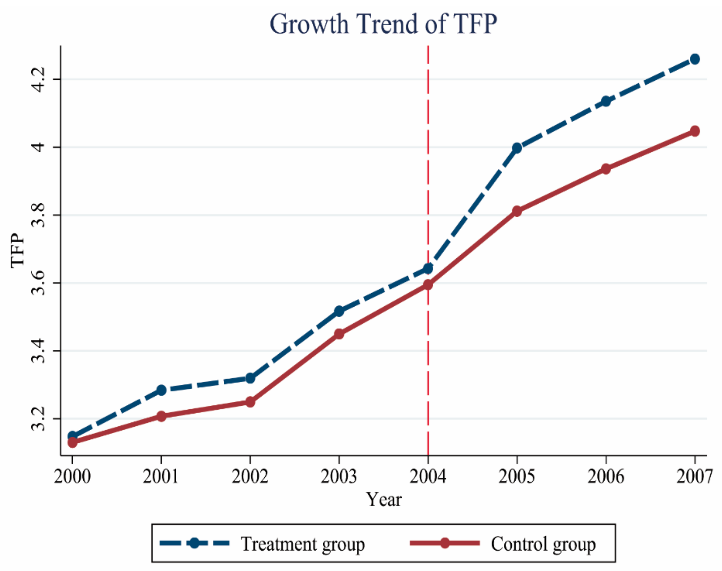
4.3.1. Parallel Trend Test

According to the results shown in Figure 3, before the responsibility agreement was signed, the TFP variation trends of the treatment group and control group are basically the same, and the parallel trend assumption is preliminarily verified. On this basis, we further introduce the interaction terms between the year dummy variables (2000–2003) and grouping variables before the introduction of this policy to test the parallel trend assumption. According to the results shown in Table 4 (1) and (2), the interaction term coefficients are not significant, indicating that there is no significant difference in the TFP of the treatment group and control group before the ETAP, which meets the parallel trend assumption.

4.3.2. Individual Time Interaction Effects

Considering that the characteristics of provinces may have an impact on TFP, we introduce provincial fixed effects to control for the characteristics of the provinces and introduce the cross-fixed effects of provinces and years to control for the characteristics of provinces that change over time. The results are shown in Table 4 columns (3) and (4). We find that the coefficient of the DID is still positively significant after taking the province characteristics into account, proving the robustness of the benchmark regression results.

4.3.3. Hysteresis Effect of Control Variables

In consideration of the possible negative relationship between the control variables and ETAP, all control variables are regressed with a lag of one stage, and the results are shown in Table 4 (5). As demonstrated in Table 4, the average treatment effect’s coefficient is 0.087, which is significant at the confidence level of 1%. As the degree of control over the variables becomes weaker, the coefficient of the DID increases a little, but its symbol and significance level are basically consistent with the benchmark results.

4.3.4. Regional Counterfactual Test

To prevent the positive effects of the ETAP from being affected by other factors, we follow the study of Ferrara et al. [67] and randomly select four provinces from the whole samples as the treatment group. It is assumed that these four provinces signed the responsibility agreements for indirect testing. This random process is repeated 500 times. Figure 4 reports the distribution of the DID regression estimation coefficients and p-values after 500 random assignments. It is found in this paper that most of the estimated coefficients of the DID are distributed near zero, and most of the p-values are greater than 0.1. These results indicate that the randomly set treatment groups do not produce policy effects, and the estimated results in this paper are unlikely to be driven by other unobservable factors.

4.3.5. PSM-DID

The PSM-DID method was proposed by Heckman et al. [68,69]. The basic idea is to find enterprise j of a province in the control group and identify the observable variables of enterprise j and enterprise i that belongs to the treatment group that match as much as possible. When matching, it is necessary to measure the distance between the two groups. While PSM, as a one-dimensional variable, has good characteristics when measuring distance [70]. The other advantage of using the PSM-DID method is that PSM can control for the deviation of the observable variables, and the use of DID can eliminate the influence of the unobserved variables, such as synchronous changes over time. In principle, the final estimates should converge regardless of the matching approach used [71]. Therefore, this paper adopts kernel matching to ensure that there is no significant difference between these two groups before the ETAP as much as possible and to reduce the endogeneity problems caused by self-selection bias. This paper calculates the change in the TFP of four provinces in the HRB and other corresponding provinces before and after the implementation of this policy and obtains the average treatment effect of the policy.
The regression results of PSM-DID are presented in Table 5. These results show that the estimated coefficients, symbols, and significance levels of different kernel matching methods are basically consistent with the benchmark results (Table 1), indicating that the ETAP has a significant positive impact on enterprise TFP, further supporting the robustness of the test results of the DID test mentioned above.

4.3.6. DDD

To eliminate industrial interference that will lead to an inconsistent TFP in the treatment group and control group, we used the DDD method for analysis. In particular, we chose CMI and non-CMI as another two groups. When the industry to which the enterprise belongs is CMI, the value is 1; otherwise, it is 0. In this paper, the DDD model is constructed as follows:
T F P i t p = β 0 + β 1 t r e a t e d i × t i m e t × i n d u s t r y p + β 2 t r e a t e d i × t i m e t + β 3 t i m e t × i n d u s t r y p + β 4 t r e a t e d i × i n d u s t r y p + β 5 t i m e t + β 6 i n d u s t r y p + β 7 t r e a t e d i + λ X + γ t + μ i + ε i t
where the definitions of the rest variables are consistent with those used in Equation (1). We are interested in the coefficient β 1 . In Table 6, columns (1)–(4) report the average treatment effect of DDD estimation. Column (1) and column (2) are the results without considering the year fixed effects. When the control variables are added, the coefficient β 1 is significantly positive. When the year fixed effects are taken into account, the coefficient β 1 decreased somewhat, but it is still statistically significant (see column (4)), which is basically consistent with the DID estimation results, indicating that the ETAP could significantly promote an improvement in TFP.

4.3.7. Sample Selection

The CIED includes only state-owned enterprises and nonstate-owned enterprises with more than 5 million CNY while nonstate-owned enterprises with less than 5 million CNY are not considered, which may lead to self-selection bias in the samples. Because large companies with strong growth ability are more likely to enter the threshold, we adjust the proportion of the existing samples in the regression by joining the probability of nonstate-owned enterprises. In this paper, five variables, the enterprise size, sales growth rate, equity ratio, return on assets, and long-term capital debt ratio, are selected to measure the probability of nonstate-owned enterprises with main revenues of more than 5 million CNY and to test whether there is sample selection bias. As demonstrated in Table 6(5), Lambda is −19.031, and the result is not significant, indicating that there is no selection bias in the model and that the benchmark regression results are robust.

4.4. Heterogeneity Analysis

4.4.1. Ownership Structure

This section studies whether there are differences in the responses of distinct enterprise ownership structures to the ETAP. Table 7 lists the regression results of these two groups. Columns (1) and (2) report the estimated values of the state-owned enterprises and nonstate-owned enterprises, respectively. This paper finds that the ETAP has no significant impact on state-owned enterprises, but it significantly promotes the growth of TFP in nonstate-owned enterprises. The result indicates that the ETAP has a greater incentive effects on nonstate-owned enterprises. The ETAP may stimulate enterprises to improve their TFP through cost inversion and innovation effects while state-owned enterprises, which are invested or controlled by government at all levels, have great advantages in terms of financial support [72] and are not sensitive to cost pressure, innovation, and improvement. In contrast, nonstate-owned enterprises are responsible for their own profits and losses. Under the pressure of policies, they have more freedom to carry out internal adjustments and have more incentives to make up for the economic losses caused by increased costs to achieve a win-win situation between environmental protection and economic performance.

4.4.2. Enterprise Scale

As indicated above, the ETAP can significantly improve the TFP of the CMI. Is there any incentive effect for enterprises of different sizes? If so, does the stimulus differ? According to the CIED standard, this paper divides the enterprises into three types by their scale for investigation. As demonstrated in Table 7, after controlling for the relevant variables, the ETAP can stimulate an increase in the TFP of small-scale enterprises, which is statistically significant, but the results are not significant for large- and medium-scale enterprises. According to the results shown in Table 8, in small-scale enterprises, the proportion of state-owned enterprises is 2.1%, which is the lowest in three types. This result is consistent with the above results of heterogeneity to some extent.

5. Conclusions and Recommendations

This paper examined the relationship between environmental regulation and enterprise TFP for Chinese CMI during the period 2000–2007 using a DID model. To validate the findings of benchmark regression, this study performed various robustness tests to throw light on this kind of relationship. The empirical results support micro evidence for the impact of environmental regulation on economic benefits, indicating that the ETAP is positively related to enterprise TFP. Analysis of robustness tests supports this argument. When considering a series of enterprise characteristic factors, a test on dynamic effects showed that there is no significant relationship between ETAP and TFP in the year of policy implementation (2004). However, this relationship possesses statistical significance from 2005 to 2007 in a positive manner. With regards to the heterogeneity test, a positive effect was only found in nonstate-owned and small-scale enterprises.
The results have important implications for policy makers in China who aspire to achieve a win-win outcome between environmental dividend and economic dividend. There is no contradiction between environmental regulation and economic development. Appropriate environmental regulation can bring sustainable production incentives to enterprises. Given that environmental regulation can effectively promote enterprise TFP, it is recommended for the further development of environmental protection strategies. The objectives and requirements of environmental regulation need to be clarified and constantly improved to achieve the goal of green and sustainable economic development. This paper found that the effects of ETAP are different between enterprises of different ownership and scales, and the government should adopt a differentiated strategy based on the ownership structure and size of enterprises rather than a one-size-fits-all approach in formulating environmental regulation. Since the ETAP has no significant impact on state-owned, large- and medium-sized enterprises, the government should pay more attention to these enterprises when formulating and implementing environmental regulation policies. The government could moderately increase the intensity of environmental regulation over large- and medium-sized enterprises. Appropriate measures can be taken to stimulate the internal adjustment of state-owned enterprises in accordance with environmental regulation. There are two main contributions of this paper. One is that an attempt was made to explore the relationship between the ETAP and enterprise TFP in HRB for the first time, which enriches research in the field of environmental regulation. The other one is that this study was conducted from a sectoral perspective. There is a one-size-fits-all phenomenon in China’s policy, which makes it vague to understand the economic effects of environmental regulation in different industries. Every industry has its own particularity, and it is of great significance to study from the perspective of different industries. Although the findings may be unique to China because of its specific historical background and industry characteristics, the research method can be easily applied to other problems. However, some limitations need to be acknowledged. We only explored the relationship between the ETAP and TFP in CMI. Yet, it is meaningful to examine the impact of the ETAP on employment, energy efficiency, and technological progress. Research on other industries is also constructive. In addition, ETAP mainly exerts pressure on government to improve the effectiveness of policy implementation, so relevant actions of government officials under the ETAP can be explored.

Author Contributions

Conceptualization, Y.Y.; methodology, Y.Y.; software, L.D.; validation, Y.L.; formal analysis, Y.Y.; investigation, Y.L.; data curation, L.D.; writing—original draft preparation, L.D.; writing—review and editing, Y.Y.; visualization, L.D.; supervision, Y.L.; project administration, Y.L.; funding acquisition, Y.L. All authors have read and agree to the published version of the manuscript.

Funding

This research was funded by Science Foundation of Zhejiang Sci-Tech University(18092252-Y), the General Project of Humanities and Social Sciences Research of the Ministry of Education of China (19YJCZH092), The National College Students’ Innovative Entrepreneurial Training Program of China (201810338043) and also sponsored by K.C. Wong Mangna Fund in Ningbo University.

Acknowledgments

We greatly appreciate useful discussion of Jing Wen and Jing Fang of Zhejiang Sci-Tech University, Yuwen Li of Zhejiang University of Finance and Economics.

Conflicts of Interest

The authors declare no conflict of interest.

Appendix A

Table A1. The comparison of total factor productivity.
StateObs.MeanS.D.MinP25P50P75Max
Control before25,3063.2701.080−7.8702.8103.3203.8408.810
Control after36,0953.8600.880−6.3903.3803.8404.3409.500
Treat before75793.3400.980−6.0302.8803.3803.8907.230
Treat after14,5384.0300.900−4.9703.46044.5908.240
Total83,5183.6601.010−7.8703.1503.6704.2309.500
Notes: Control before means the control group before the implementation of the policy, Control after means the control group after the implementation of the policy, Treat before means the treat group before the implementation of the policy, Treat after means the treat group after the implementation of the policy.

References

  1. Ministry of Ecology and Environment of the People’s Republic of China. China Ecological Environment Bulletin 2018. Available online: http://www.mee.gov.cn/hjzl/zghjzkgb/lnzghjzkgb/201905/P020190619587632630618.pdf (accessed on 21 February 2020).
  2. Schlenker, W.; Walker, W.R. Airports, air pollution, and contemporaneous health. Rev. Econ. Stud. 2016, 83, 768–809. [Google Scholar] [CrossRef] [Green Version]
  3. Zeng, D.Z.; Zhao, L. Pollution havens and industrial agglomeration. J. Environ. Econ. Manag. 2009, 58, 141–153. [Google Scholar] [CrossRef] [Green Version]
  4. National Bureau of Statistics. Study Report 2004 for Green National Economic Accounting. Available online: http://www.stats.gov.cn/ztjc/zthd/xzgcl60zn/xzg60ntjdsj/200909/t20090921_68907.htm (accessed on 16 January 2020).
  5. Shapiro, J.S.; Walker, R. Why is pollution from US manufacturing declining? The roles of trade, regulation, productivity, and preferences. Am. Econ. Rev. 2018, 108, 3814–3854. [Google Scholar] [CrossRef] [Green Version]
  6. The centre government of the People’s Republic of China. Report of the State Council on 2019. Available online: http://www.gov.cn/premier/2019-03/16/content_5374314.htm (accessed on 10 September 2019).
  7. Jia, R. Pollution for Promotion; 21st Century China Center: San Diego, CA, USA, 2017. [Google Scholar]
  8. Yuan, B.; Ren, S.; Chen, X. Can environmental regulation promote the coordinated development of economy and environment in China’s manufacturing industry?–A panel data analysis of 28 sub-sectors. J. Clean. Prod. 2017, 149, 11–24. [Google Scholar] [CrossRef]
  9. Cheng, Z.; Li, L.; Liu, J. The emissions reduction effect and technical progress effect of environmental regulation policy tools. J. Clean. Prod. 2017, 149, 191–205. [Google Scholar] [CrossRef]
  10. Chen, Y.J.; Li, P.; Lu, Y. Career concerns and multitasking local bureaucrats: Evidence of a target-based performance evaluation system in China. J. Dev. Econ. 2018, 133, 84–101. [Google Scholar] [CrossRef]
  11. Shen, M.; Yang, Y. The water pollution policy regime shift and boundary pollution: Evidence from the change of water pollution levels in China. Sustainability 2017, 9, 1469. [Google Scholar] [CrossRef] [Green Version]
  12. Qi, Y.; Lu, H.; Zhang, N. Will environmental regulation help reduce pollution and improve efficiency?: Evidence from a Quasi-experiment in Major Cities for pollution control. In A New Era; He, D., Wang, C., Eds.; Palgrave Macmillan: Singapore, 2019; pp. 237–268. ISBN 978-981-10-8356-3. [Google Scholar]
  13. She, Y.; Liu, Y.; Jiang, L.; Yuan, H. Is China’s River Chief Policy effective? Evidence from a quasi-natural experiment in the Yangtze River Economic Belt, China. J. Clean. Prod. 2019, 220, 919–930. [Google Scholar] [CrossRef]
  14. Pu, Z.; Fu, J. Economic growth, environmental sustainability and China mayors’ promotion. J. Clean. Prod. 2018, 172, 454–465. [Google Scholar] [CrossRef]
  15. Wang, C.; Wu, J.J.; Zhang, B. Environmental regulation, emissions and productivity: Evidence from Chinese COD-emitting manufacturers. J. Environ. Econ. Manag. 2018, 92, 54–73. [Google Scholar] [CrossRef]
  16. Li, Y.; Tang, Y.; Wang, K.; Zhao, Q. Environmental regulation and China’s regional innovation output-empirical research based on spatial durbin model. Sustainability 2019, 11, 5602. [Google Scholar] [CrossRef]
  17. Yang, Y.; Wen, J.; Li, Y. The Impact of Environmental Information Disclosure on the Firm Value of Listed Manufacturing Firms: Evidence from China. Int. J. Environ. Res. Public Health 2020, 17, 916. [Google Scholar] [CrossRef] [PubMed] [Green Version]
  18. Zhang, G.; Zhang, P.; Zhang, Z.G.; Li, J. Impact of environmental regulations on industrial structure upgrading: An empirical study on Beijing-Tianjin-Hebei region in China. J. Clean. Prod. 2019, 238, 117848. [Google Scholar] [CrossRef]
  19. Wang, X.; Shao, Q. Non-linear effects of heterogeneous environmental regulations on green growth in G20 countries: Evidence from panel threshold regression. Sci. Total Environ. 2019, 660, 1346–1354. [Google Scholar] [CrossRef]
  20. Hancevic, P.I. Environmental regulation and productivity: The case of electricity generation under the CAAA-1990. Energy Econ. 2016, 60, 131–143. [Google Scholar] [CrossRef]
  21. Li, C. How does environmental regulation affect different approaches of technical progress?—Evidence from China’s industrial sectors from 2005 to 2015. J. Clean. Prod. 2019, 209, 572–580. [Google Scholar] [CrossRef]
  22. Chen, B.; Cheng, Y.S. The impacts of environmental regulation on industrial activities: Evidence from a quasi-natural experiment in Chinese prefectures. Sustainability 2017, 9, 571. [Google Scholar] [CrossRef] [Green Version]
  23. Shi, X.; Xu, Z. Environmental regulation and firm exports: Evidence from the eleventh Five-Year Plan in China. J. Environ. Econ. Manag. 2018, 89, 187–200. [Google Scholar] [CrossRef]
  24. Gray, W.B.; Shadbegian, R.J. Plant vintage, technology, and environmental regulation. J. Environ. Econ. Manag. 2003, 46, 384–402. [Google Scholar] [CrossRef] [Green Version]
  25. Lanoie, P.; Patry, M.; Lajeunesse, R. Environmental regulation and productivity: Testing the porter hypothesis. J. Product. Anal. 2008, 30, 121–128. [Google Scholar] [CrossRef]
  26. Löfgren, A.; Wråke, M.; Hagberg, T.; Roth, S. The Effect of EU-ETS on Swedish Industry’s Investment in Carbon Mitigating Technologies; University of Gothenburg: Gothenburg, Sweden, 2013. [Google Scholar]
  27. Tombe, T.; Winter, J. Environmental policy and misallocation: The productivity effect of intensity standards. J. Environ. Econ. Manag. 2015, 72, 137–163. [Google Scholar] [CrossRef]
  28. Banerjee, S.N. The Impact of EPA Regulations on the US Manufacturing Industry. Southwest. Econ. Rev. 2016, 43, 151–163. [Google Scholar]
  29. Cohen, M.A.; Tubb, A. The Impact of Environmental Regulation on Firm and Country Competitiveness: A Meta-Analysis of the Porter Hypothesis. J. Chem. Inf. Model. 2017, 53, 1689–1699. [Google Scholar]
  30. Porter, M.E.; Van der Linde, C. Toward a new conception of the environment-competitiveness relationship. J. Econ. Perspect. 1995, 9, 97–118. [Google Scholar] [CrossRef]
  31. Cole, M.A.; Elliott, R.J.R.; Shimamoto, K. Industrial characteristics, environmental regulations and air pollution: An analysis of the UK manufacturing sector. J. Environ. Econ. Manag. 2005, 50, 121–143. [Google Scholar] [CrossRef]
  32. Testa, F.; Iraldo, F.; Frey, M. The effect of environmental regulation on firms’ competitive performance: The case of the building & construction sector in some EU regions. J. Environ. Manag. 2011, 92, 2136–2144. [Google Scholar]
  33. Rubashkina, Y.; Galeotti, M.; Verdolini, E. Environmental regulation and competitiveness: Empirical evidence on the Porter Hypothesis from European manufacturing sectors. Energy Policy 2015, 83, 288–300. [Google Scholar] [CrossRef] [Green Version]
  34. Hamamoto, M. Environmental regulation and the productivity of Japanese manufacturing industries. Resour. Energy Econ. 2017, 28, 299–314. [Google Scholar] [CrossRef]
  35. Morales-Lage, R.; Bengochea-Morancho, A.; Martínez-Zarzoso, I. Does Environmental Policy Stringency Foster Innovation and Productivity in OECD Countries? University of Göttingen: Göttingen, Germany, 2016. [Google Scholar]
  36. Albrizio, S.; Kozluk, T.; Zipperer, V. Environmental policies and productivity growth: Evidence across industries and firms. J. Environ. Econ. Manag. 2017, 81, 209–226. [Google Scholar] [CrossRef]
  37. Nguyen, H.T.T.; Minh, N.K.; Quoc, T.N. The Role of Environmental Regulations and Innovation in TFP Convergence: Evidence from Manufacturing SMEs in Vietnam; The United Nations University World Institute for Development Economics Research: Helsinki, Finland, 2017; ISBN 978-92-9256-316-5. [Google Scholar]
  38. Qiu, L.D.; Zhou, M.; Wei, X. Regulation, innovation, and firm selection: The porter hypothesis under monopolistic competition. J. Environ. Econ. Manag. 2018, 92, 638–658. [Google Scholar] [CrossRef]
  39. Cordella, T.; Devarajan, S. Firms’ and states’ responses to laxer environmental standards. J. Environ. Econ. Manag. 2019, 98, 102275. [Google Scholar] [CrossRef] [Green Version]
  40. Jaffe, A.B.; Peterson, S.R.; Portney, P.R.; Stavins, R.N. Environmental regulation and the competitiveness of US manufacturing: what does the evidence tell us? J. Econ. Lit. 1995, 33, 132–163. [Google Scholar]
  41. Palmer, K.; Oates, W.E.; Portney, P.R. Tightening environmental standards: The Benefit-Cost or the No-Cost paradigm? Econ. Costs Conseq. Environ. Regul. 2018, 9, 435–448. [Google Scholar] [CrossRef]
  42. Alpay, E.; Kerkvliet, J.; Buccola, S. Productivity growth and environmental regulation in Mexican and US food manufacturing. Am. J. Agric. Econ. 2002, 84, 887–901. [Google Scholar] [CrossRef]
  43. Lange, I.; Redlinger, M. Effects of stricter environmental regulations on resource development. J. Environ. Econ. Manag. 2019, 96, 60–87. [Google Scholar] [CrossRef] [Green Version]
  44. Hu, D.; Wang, Y.; Li, Y. How Does Open Innovation Modify the Relationship between Environmental Regulations and Productivity? Bus. Strateg. Environ. 2017, 26, 1132–1143. [Google Scholar] [CrossRef]
  45. Peng, J.; Xiao, J.; Zhang, L.; Wang, T. The impact of China’s ‘Atmosphere Ten Articles’ policy on total factor productivity of energy exploitation: Empirical evidence using synthetic control methods. Resour. Policy 2020, 65, 101544. [Google Scholar] [CrossRef]
  46. He, G.; Wang, S.; Zhang, B. Leveraging Political Incentives for Environmental Regulation: Evidence from Chinese Manufacturing Firms; Centre for Economic Policy Research: London, UK, 2019. [Google Scholar]
  47. Liu, Z.; Mao, X.; Tu, J.; Jaccard, M. A comparative assessment of economic-incentive and command-and-control instruments for air pollution and CO2 control in China’s iron and steel sector. J. Environ. Manag. 2014, 144, 135–142. [Google Scholar] [CrossRef]
  48. Zhao, X.; Zhao, Y.; Zeng, S.; Zhang, S. Corporate behavior and competitiveness: Impact of environmental regulation on Chinese firms. J. Clean. Prod. 2015, 86, 311–322. [Google Scholar] [CrossRef]
  49. Zhao, X.; Liu, C.; Yang, M. The effects of environmental regulation on China’s total factor productivity: An empirical study of carbon-intensive industries. J. Clean. Prod. 2018, 179, 325–334. [Google Scholar] [CrossRef]
  50. Filippini, M.; Geissmann, T.; Karplus, V.J.; Zhang, D. The productivity impacts of energy efficiency programs in developing countries: Evidence from iron and steel firms in China. China Econ. Rev. 2020, 59, 101364. [Google Scholar] [CrossRef]
  51. Xie, R.H.; Yuan, Y.J.; Huang, J.J. Different types of environmental regulations and heterogeneous influence on “green” productivity: Evidence from China. Ecol. Econ. 2017, 132, 104–112. [Google Scholar] [CrossRef]
  52. Ministry of Ecology and Environment of the People’s Republic of China. Available online: http://www.mee.gov.cn/gkml/sthjbgw/qt/200910/t20091023_179813.htm (accessed on 16 January 2020).
  53. Ministry of Ecology and Environment of the People’s Republic of China. Available online: http://www.mee.gov.cn/gkml/sthjbgw/qt/200910/t20091023_179992.htm (accessed on 16 January 2020).
  54. Leiter, A.M.; Parolini, A.; Winner, H. Environmental regulation and investment: Evidence from European industry data. Ecol. Econ. 2011, 70, 759–770. [Google Scholar] [CrossRef]
  55. Chung, S. Environmental regulation and foreign direct investment: Evidence from South Korea. J. Dev. Econ. 2014, 108, 222–236. [Google Scholar] [CrossRef]
  56. Wang, Y.; Shen, N. Environmental regulation and environmental productivity: The case of China. Renew. Sustain. Energy Rev. 2016, 62, 758–766. [Google Scholar] [CrossRef]
  57. Li, R.; Ramanathan, R. Exploring the relationships between different types of environmental regulations and environmental performance: Evidence from China. J. Clean. Prod. 2018, 196, 1329–1340. [Google Scholar] [CrossRef]
  58. Olley, G.S.; Pakes, A. The dynamics of productivity in the telecommunications equipment industry. Econometrica 1996, 64, 1263–1297. [Google Scholar] [CrossRef]
  59. Wang, X.; Luo, Z.; Wang, T.; Huang, Z. The impact of privatization on TFP: A quasi-experiment in China. Ann. Econ. Financ. 2017, 18, 53–71. [Google Scholar]
  60. Bernard, A.B.; Moxnes, A.; Saito, Y.U. Production networks, geography, and firm performance. J. Polit. Econ. 2019, 127, 639–688. [Google Scholar] [CrossRef] [Green Version]
  61. Zhang, Q.; Yu, Z.; Kong, D. The real effect of legal institutions: Environmental courts and firm environmental protection expenditure. J. Environ. Econ. Manag. 2019, 98, 102254. [Google Scholar] [CrossRef]
  62. Cai, H.; Liu, Q.; Xiao, G. Does competition encourage unethical behavior? The case of corporate profit hiding in China. Econ. J. 2009, 119, 764–795. [Google Scholar] [CrossRef]
  63. Brandt, L.; Van Biesebroeck, J.; Zhang, Y. Creative accounting or creative destruction? Firm-level productivity growth in Chinese manufacturing. J. Dev. Econ. 2012, 97, 339–351. [Google Scholar] [CrossRef] [Green Version]
  64. Feenstra, R.C.; Li, Z.; Yu, M. Exports and credit constraints under incomplete information: Theory and evidence from China. Rev. Econ. Stat. 2014, 96, 729–744. [Google Scholar] [CrossRef]
  65. Jacobson, L.S.; LaLonde, R.J.; Sullivan, D.G. Earnings losses of displaced workers. Am. Econ. Rev. 1993, 83, 685–709. [Google Scholar]
  66. Li, P.; Lu, Y.; Wang, J. Does flattening government improve economic performance? Evidence from China. J. Dev. Econ. 2016, 123, 18–37. [Google Scholar] [CrossRef]
  67. Ferrara, E.; Chong, A.; Duryea, S. Soap operas and fertility: Evidence from Brazil. Am. Econ. J. Appl. Econ. 2012, 4, 1–31. [Google Scholar] [CrossRef] [Green Version]
  68. Heckman, J.J.; Ichimura, H.; Todd, P.E. Matching as an econometric evaluation estimator: Evidence from evaluating a job training programme. Rev. Econ. Stud. 1997, 64, 605–654. [Google Scholar] [CrossRef]
  69. Heckman, J.J.; Ichimura, H.; Todd, P. Matching as an econometric evaluation estimator. Rev. Econ. Stud. 1998, 65, 261–294. [Google Scholar] [CrossRef]
  70. Rosenbaum, P.R.; Rubin, D.B. The central role of the propensity score in observational studies for causal effects. Biometrika 1983, 70, 41–55. [Google Scholar] [CrossRef]
  71. Vandenberghe, V.; Robin, S. Evaluating the effectiveness of private education across countries: A comparison of methods. Labour Econ. 2004, 11, 487–506. [Google Scholar] [CrossRef]
  72. Allen, F.; Qian, J.; Qian, M. Law, finance, and economic growth in China. J. Financ. econ. 2005, 77, 57–116. [Google Scholar] [CrossRef] [Green Version]
Figure 1. Characteristics of wastewater discharged by the textile industry
Sustainability 12 01696 g001
Figure 2. TFP Kdensity. The kdensity curve of total factor productivity.
Sustainability 12 01696 g002
Figure 3. Parallel trend test.
Sustainability 12 01696 g003
Figure 4. Estimated distribution of the coefficient of treated×time.
Sustainability 12 01696 g004
Table 1. Descriptive statistics of the variables.
VariablesObs.MeanS.D.MinP25P50P75Max
tfp83,5183.6601.010−7.8703.1503.6704.2309.500
cs85,0869.8401.09009.1109.74010.4816.27
nl84,9220.02000.140−0.9400001
clr85,31931.69190.405.65012.6727.5624,698
eo85,6110.02000.15000001
ri85,0860.68052.80−52200.08000.1900.40010,068
cost84,5706.6201.29005.8506.6307.42013.34
tax85,0860.04002.950−0.5300.01000.02000.0400857
export85,0860.5000.460000.55011
fi84,9220.1400.320−9.8500001.170
Table 2. Benchmark regression results.
Variables(1)(2)(3)(4)
TFPTFPTFPTFP
treated×time0.568 ***0.287 ***0.112 ***0.031 ***
(41.882)(31.322)(7.719)(3.084)
Constant3.564 ***−3.827 ***3.345 ***−3.242 ***
(1098.504)(−112.939)(360.084)(−93.831)
ControlNYNY
Year FENNYY
Observations83,51882,26983,51882,269
R-squared0.0300.4950.1590.535
Note: ***, **, and * indicate statistical significance at the 1%, 5%, and 10% levels, respectively. The t statistics are in parentheses.
Table 3. Test results for the dynamic effect.
Variables(1)(2)(3)(4)
TFPTFPTFPTFP
current0.190 ***0.165 ***−0.0160.004
(11.448)(14.672)(−0.885)(0.304)
post_10.557 ***0.317 ***0.134 ***0.053 ***
(33.359)(27.811)(7.339)(4.174)
post_20.720 ***0.327 ***0.167 ***0.024 *
(43.378)(28.667)(9.174)(1.939)
post_30.909 ***0.396 ***0.198 ***0.049 ***
(53.898)(33.704)(10.622)(3.780)
Constant3.555 ***−3.701 ***3.346 ***−3.235 ***
(1111.350)(−107.532)(360.557)(−93.416)
ControlNYNY
Year FENNYY
Observations83,51882,26983,51882,269
R-squared0.0610.4990.1610.535
Note: Current represents the interaction terms year2004×treated. When year=2004, year2004=1, otherwise, it equals 0. Post_* represents the interaction terms between the year dummy variables (2005–2007) and grouping variables after the introduction of this policy. For example, post_1 reflects the results for year2005×treated. When year=2005, year2005=1, otherwise, it equals 0 (the same is true for the tables below). ***, **, and * indicate statistical significance at the 1%, 5%, and 10% levels, respectively. The t statistics are in parentheses.
Table 4. Robustness test(I).
Variables(1)(2)(3)(4)(5)
Parallel TrendPro FeatureL.Control
TFPTFPTFPTFPTFP
treated×time0.155 ***0.033 **0.031 ***0.356 ***0.087 ***
(8.088)(2.499)(3.087)(5.178)(5.732)
pre_4−0.027−0.016
(−0.979)(−0.863)
pre_30.013−0.013
(0.552)(−0.747)
pre_2−0.029−0.016
(−1.309)(−1.044)
current−0.180 ***−0.038 ***
(−11.600)(−3.578)
Constant3.352 ***−3.230 ***−3.233 ***−2.861 ***1.532 ***
(296.105)(−92.605)(−89.098)(−69.503)(27.100)
Year FEYYYNY
ControlNYYYN
L.ControlNNNNY
Pro FENNYNN
Year×Pro FENNYYN
Observations83,51882,26982,26982,26955,709
R-squared0.1610.5350.5350.5510.188
Note: Pre_* represents the interaction terms between the year dummy variables (2000−2003) and grouping variables before the introduction of this policy. For example, pre_4 refers to the interaction year2000×treated. When year=2000, year2000=1; otherwise, it equals 0. L.control represents control variables which are lagged for one period (the same is true for the tables below). ***, **, and * indicate statistical significance at the 1%, 5%, and 10% levels, respectively. The t statistics are in parentheses.
Table 5. Robustness test (II).
Variables(1)(2)(3)(4)(5)(6)
ProbitLogit
EpanechnikovEpanechnikovGaussianBiweightUniformTricube
treated×time0.193 ***0.188 ***0.172 ***0.193 ***0.178 ***0.185 ***
(11.270)(10.060)(10.254)(10.548)(10.322)(10.278)
treated−0.023 **−0.020 *0.012−0.027 **−0.007−0.014
(−2.059)(−1.696)(1.095)(−2.227)(−0.528)(−1.171)
time0.498 ***0.500***0.516***0.496 ***0.508 ***0.504 ***
(57.146)(58.578)(63.497)(58.145)(61.887)(59.058)
cons3.381 ***3.380 ***3.348 ***3.386 ***3.368 ***3.373 ***
(584.883)(658.459)(642.045)(594.193)(623.108)(608.095)
Bs reps500500500500500500
ControlYYYYYY
Observations53,81353,79553,88753,85753,78753,901
Notes: ***, **, and * indicate statistical significance at the 1%, 5%, and 10% levels, respectively. The t statistics are in parentheses.
Table 6. Robustness test (III).
Variables(1)(2)(3)(4)(5)
DDDHeckman
TFPTFPTFPTFPTFP
treated×time×industry−0.0070.033 **−0.0080.032 **
(−0.360)(2.304)(−0.414)(2.213)
treated×time0.115 ***−0.0010.112 ***0.0010.232
(28.642)(−0.412)(28.526)(0.382)(1.165)
industry×time0.191 ***0.311 ***0.189 ***0.307 ***
(19.466)(43.113)(19.710)(42.595)
treated×industry−0.041−0.066 ***−0.040−0.065 ***
(−1.462)(−3.174)(−1.443)(−3.132)
time0.271 ***−0.017 ***0.600 ***0.059 ***
(128.284)(−10.336)(172.021)(20.754)
industry0.284 ***0.214 ***0.277 ***0.215 ***
(20.332)(20.848)(20.287)(20.992)
treated−0.1570.476 **−0.1150.496 **
(−0.555)(2.189)(−0.416)(2.286)
Constant2.792 ***−3.961 ***2.730 ***−3.725 ***
(34.591)(−62.430)(34.541)(−58.738)
Lambda −19.031
(−1.365)
Year FENNYYN
ControlNYNYY
Observations1,763,3001,713,8971,763,3001,713,89757,065
R-squared0.0260.3300.0670.333
Notes: ***, **, and * indicate statistical significance at the 1%, 5%, and 10% levels, respectively. The t statistics are in parentheses.
Table 7. Heterogeneity test.
Variables(1)(2)(3)(4)(5)
Enterprise OwnershipEnterprise Scale
State-OwnedNon-State-OwnedLargeMediumSmall
TFPTFPTFPTFPTFP
treated×time0.0240.031 ***−0.050−0.0220.037 ***
(0.214)(3.080)(−0.403)(−0.558)(2.951)
Constant−5.571 ***−3.203 ***−5.013 ***−5.193 ***−3.386 ***
(−19.571)(−91.987)(−4.985)(−24.642)(−77.478)
Year FEYYYYY
Observations160480,665346477756,927
R-squared0.5690.5350.6960.5640.545
Notes: ***, **, and * indicate statistical significance at the 1%, 5%, and 10% levels, respectively. The t statistics are in parentheses.
Table 8. Tabulation of ownership structure and enterprise size.
Scale
LargeMediumSmallTotal
Ownership structureNonstate-owned305467658,07063,051
State-owned5518412351474
Total360486059,30564,525
State-owned/Total0.1530.0380.0210.023

