Optimization of Green Fresh Food Logistics with Heterogeneous Fleet Vehicle Route Problem by Improved Genetic Algorithm

Abstract

In order to reduce the distribution cost of fresh food logistics and achieve the goal of green distribution at the same time, the Green Fresh Food Logistics with Heterogeneous Fleet Vehicle Route Problem (GFLHF-VRP) model is established. Based on the particularity of the model, an improved genetic algorithm called Genetic Algorithm with Adaptive Simulated Annealing Mutation (GAASAM) is proposed in which the mutation operation is upgraded to a simulated annealing mutation operation and its parameters are adjusted by the adaptive operation. The experimental results show that the proposed GAASAM can effectively solve the vehicle routing problem of the proposed model, achieve better performance than the genetic algorithm, and avoid falling into a local optimal trap. The distribution routes obtained by GAASAM are with lower total distribution cost, and achieve the goal of green distribution in which energy, fuel consumption and carbon emissions are reduced at the same time. On the other hand, the proposed GFLHF-VRP and GAASAM can provide a reliable distribution route plan for fresh food logistics enterprises with multiple types of distribution vehicles in real life, which can further reduce the distribution cost and achieve a greener and more environment-friendly distribution solution. The results of this study also provide a managerial method for fresh food logistics enterprises to effectively arrange the distribution work with more social responsibility.

1. Introduction

In recent years, global warming is an issue that cannot be ignored, and China’s carbon emissions have also received widespread attention [1]. Moreover, at the United Nations Climate Conference in Copenhagen, China promised to reduce carbon emissions per unit of GDP to 50–60% of the 2005 level by 2020; however, the carbon emissions in China are at a high level, and most of it comes from fossil fuel consumption [2]. The concept of low-carbon, that is, “low energy consumption, low pollution, and low emissions” [3] should be universally implemented in China.

With the improvement of quality of life and social economy, people’s demand for fresh foods is increasing, and fresh food logistics is rapidly developing for it [4]. Fresh food logistics is a logistics for fresh food products with distribution vehicles equipped with a freezing chamber and a refrigerator to keep the products in a low temperature [5], and the quality of the products depends on the time of delivery, the distribution vehicles are supposed to deliver the products from the distribution center to the customers on time in the fresh food logistics [6]. Nowadays, more and more people are enjoying the benefits from the fresh food logistics. However, the fresh food logistics is a special logistics mode with high energy consumption and high carbon emissions [7,8]. Due to the need to control the temperature of the freezing chamber, the refrigeration consumes electric energy resulting in a higher cost [9]; moreover, the fuel consumption and the carbon emission of the vehicle in fresh food logistics are higher than those of the ordinary logistics [10], which will cause more damage to the environment. In Logistics 4.0, the sustainability and the pollution to the environment in the logistics are focused, restrictions in damages to environment may force companies to adjust their logistics operations [11,12]. Therefore, for fresh food logistics, not only the total distribution cost should be reduced, but also fuel consumption, refrigeration’s energy consumption, and carbon emissions in distribution should be reduced to realize the green distribution.

Based on the previous researches, the fuel consumption cost related to the fuel consumption, the refrigeration’s energy consumption and the carbon emission cost of distribution vehicles are introduced into the existing vehicle routing model for the fresh food logistics, and then a Green Fresh-Food Logistics with Heterogeneous Fleet Vehicle Route Problem (GFLHF-VRP) model considering the reduction of the distribution cost and the damage to the environment has been proposed.

2. Literature Review

The purpose of this paper is to propose an optimal distribution route for the fresh food logistics considering the reduction of total distribution cost and damage to the environment including the fuel consumption, refrigeration’s energy consumption and carbon emissions. Therefore, a number of literatures in the area of Green logistics, VRP models considering the damage to the environment and VRP models for fresh food logistics have been reviewed.

2.1. Green Logistics

Strandhagen et al. proposed the importance of maintaining sustainability and reducing negative impact on the environment in logistics 4.0 [11]; Boenzi et al. evaluated the overall impact due to all energy-consumptive factors of the warehousing activities and provide the best logistic solutions with lower environmental impact [13]; Facchini et al. built a maturity model for Logistics 4.0 focusing on the environmental factors [12]; and Facchini et al. analyzed the optimal warehouse layout for agricultural and food collecting centers, and built an analytical model to minimize the travelling time of the goods from picking to delivery area with consideration of carbon footprint and sustainability [14].

2.2. VRP Models Considering the Damage to the Environment

To build the GFLHF-VRP model, a series of researches about the G-VRP that considers the damage to the environment have been reviewed. Kuo et al. proposed an idea of optimizing the VRP by minimizing the fuel consumption to protect the environment and achieve the goal of green transportation [15]. Bektaş et al. presented the pollution-routing problem as an extension of the classical VRP with more comprehensive objective function that accounts not just for the travel distance, but also for the amount of greenhouse emissions, fuel, travel times and their costs [16]. Erdoğan et al. proposed the Green Vehicle Routing Problem (G-VRP) focusing on the negative influence on the environment in the distribution to realize the green distribution [17]. Koç et al. realized the reduction of fuel consumptions and carbon emissions of the distribution through using multi-type vehicles for the distribution planning [18]; moreover, Xiao et al. conducted the further research on the reduction of the fuel consumption in the distribution by vehicle route planning [19]. Kwon et al. concentrated on the carbon emission in the distribution and proposed a vehicle route planning method with Heterogeneous fixed fleet of vehicles to propose the route plan, and proved that the amount of carbon emission can be reduced without increasing total costs [20]. GFLHF-VRP model building with multi-type vehicles was inspired by Kwon’s work. Bortolini et al. proposed the sustainable distribution route planning method including the multi-objective optimization of cost, delivery time and carbon footprint in the fresh food logistics [21]. Niu et al. proposed a green VRP with time windows by minimizing total cost including the fuel cost, carbon emissions cost and driver cost to realize the reduction of the negative influence to the environment [22]. Naderipour et al. proposed an open time dependent VRP model that considers the minimization of CO${}_2$, NO${}_x$ and CO emissions [23].

2.3. VRP Models for Fresh Food Logistics

A series of researches about the VRP model in fresh food logistics with cold chain have been conducted in recent years. To build GFLHF-VRP model that include as many aspects as possible, a number of related researches on fresh logistics and cold chain logistics are reviewed. Hsu et al. proposed the VRP model with time windows for fresh food logistics firstly, in which the randomness of the perishable fresh food was considered [24]. Osvald et al. integrated multiple costs and established a vehicle route planning model in the logistics distribution of perishable fresh food [25]. Wu et al. worked further in VRP model for fresh food logistics, and proposed the improve genetic algorithm [26]. Amorim et al. built the VRP model for perishable food with more details, which is a heterogeneous fleet site dependent vehicle routing problem with multiple time windows [27]. Yantong et al. studied the VRP model in routing planning for perishable food and considered the quality of the product which decreases as transportation time increases [28]. Wang et al. considered the difference of the energy consumption of refrigeration is opened and closed in fresh food logistics [29]. Shukla et al. integrated the transportation cost, damage cost of good and overtime penalty cost as the overall optimization goal of the model [30]. Chen et al. considered the factors of carbon emission, fuel cost, freshness degradation of products and time windows penalty cost in fresh food logistics [7].

In the above mentioned literatures, there have been many studies related to fresh food logistics and many factors have been considered. However, few researchers have proposed models to solve the problem of green vehicle route planing for fresh food logistics that effectively reduces the damage to the environmental and the distribution costs simultaneously. Thus, the GFLHF-VRP model is proposed, where most of the factors of fresh food logistics are considered to provide an environment-friendly and low cost distribution route. The comparison of the factors considered in GFLHF-VRP model and the factors considered in other researchers’ models for fresh food logistics is shown in

Table 1. Comparison of the factors considered in the proposed models of fresh food logistics.

Studies	Fuel Consumption	Refrigeration’s Energy Consumption	Carbon Emission	Time Windows	Product Damage	Hetero- geneous Fleets
Hsu et al. [24]	-	-	-	✓	-	-
Osvald et al. [25]	-	-	-	✓	✓	-
Wu et al. [26]	-	-	-	✓	-	-
Amorim et al. [27]	-	-	-	✓	-	✓
Yantong et al. [28]	-	-	-	-	✓	-
Shukla et al. [30]	-	-	-	✓	✓	-
Chen et al. [7]	✓	✓	-	✓	✓	-
Wang et al. [29]	✓	✓	✓	✓	✓	-
This study	✓	✓	✓	✓	✓	✓

, which shows that GFLHF-VRP model is comprehensive and close to the practical application.

3. Model Formulation

3.1. Model Description

In order to achieve environment-friendly and low cost distribution vehicle route planning for fresh food logistics, the GFLHF-VRP model considering energy saving and emission reduction is established, in which multi-type vehicles are available to be used. In this model, the total distribution cost should be lowered, and the fuel consumption, refrigeration’s energy consumption and carbon emission in the distribution process be reduced as much as possible. The detailed assumption of the model are as follows:

• There is only one distribution center, and the distribution center has vehicles of different types;
• Each type of vehicle has its own maximum load, fixed cost, fuel consumption, refrigeration energy consumption and the coefficient of carbon emission;
• The salary of the driver is included in the fixed cost of the distribution vehicle;
• The quality of fresh food is related to delivery time and temperature;
• The delivery vehicle shall arrive at the customer point within the time window specified by the customer. If it arrives at the customer point after the time window, it shall bear the cost of overtime punishment;
• The demand of any customer is not greater than the maximum load of any vehicle;
• The battery supplies the refrigeration equipment of the vehicle; and capacity of batteries is set to be enough for distribution, the situation that the vehicle runs without power will not be considered;
• All vehicles should depart from the distribution center and finally return to the distribution center;
• Vehicles shall not be overloaded;
• All vehicles run at a uniform speed.

3.2. Parameters and Variable Definition

The mathematical model of the proposed model is established as follows. Assuming that D is the set of customer points, V is the total set, and $V=0\bigcup D=\{0,1,\dots ,n\}$ where 0 is the distribution center and n is the number of the customers; M is the set of the types of vehicle, and $M=\{0,1,\dots ,h\}$ where h is the number of the types of vehicle. The relevant variables and parameters of the model are shown in

Table 2. Parameters and variables.

Notations	Description
$\beta$	Penalty cost per unit overtime
$\theta$	Sensitivity of fresh food quality to delivery time
$C^m$	Maximum load of the m-type distribution vehicle, $m\in M$
$K^m$	Quantity of m-type vehicles available in the distribution center, $m\in M$
${\rho }^m$	Fixed cost of m-type distribution vehicles, $m\in M$
${\epsilon }^m$	Fuel consumption per unit distance of the m-type vehicle, $m\in M$
$d_{i,j}$	Travel distance from point i to point j, $i,j\in V$
$t_{i,j}$	Travel time from point i to point j, $i,j\in V$
$g_i$	Demand of customer i, $i\in D$
$a_i$	Service time of the customer point i, $i\in D$
$Q_c^m$	Energy consumption in refrigeration per unit time, when the door of freezing chamber of m-type vehicle is opened, $m\in M$
$Q_o^m$	Energy consumption in refrigeration per unit time, when the door of freezing chamber of m-type vehicle is closed, $m\in M$
$E^m$	Carbon emission coefficient for unit fuel consumption of m-type vehicle, $m\in M$
$C_l$	Cost per unit damaged fresh food
$C_p$	Cost per unit fuel
$C_q$	Cost per unit energy consumption in refrigeration
$C_e$	Environmental cost of unit carbon emission
$w_i$	Arrival time for distribution vehicle to customer point i, $i\in D$
$[e_i,l_i]$	Time window of the customer point i in which $e_i$ is the early-arrival time, $l_i$ is the late-arrival time
$x_{i,j}^{m,k}$	Route selection variable; $x_{i,j}^{m,k}=1$, if the m-type vehicle k travel from point i to point j, $x_{i,j}^{m,k}=0$, otherwise; $i,j\in V,m\in M,k\in \{1,2,\dots ,K^m\}$

:

3.3. Cost Analysis in GFLHF-VRP Model

The total distribution cost in GFLHF-VRP model includes fixed cost, damage cost, overtime penalty cost, fuel consumption cost, refrigeration’s energy cost and carbon emission cost, among which fuel consumption cost, refrigeration’s energy cost and carbon emission cost are related to energy conservation and emission reduction which are the key to achieve the environment-friendly distribution of fresh food logistics; fixed cost, damage cost and overtime penalty cost are basic costs in the basic VRP for fresh food logistics.

3.3.1. Fixed Cost

Fixed costs are the costs of using vehicles for distribution tasks. The fixed costs of various types of vehicles are different, and the calculation method of fixed cost is shown as follows:

$$C_1=\sum _{m=1}^h\sum _{k=1}^{K^m}\sum _{j=1}^n{\rho }^m·x_{0,j}^{m,k}$$

(1)

3.3.2. Damage Cost

In the process of distribution, the quality of fresh food will be reduced to a certain extent due to the influence of time [31], thus, the damage cost is generated. The calculation method of damage cost is shown as follows:

$$C_2=C_l\sum _{i=1}^n{g}_i·e^{-\theta w_i}$$

(2)

3.3.3. Overtime Penalty Cost

If the distribution vehicles arrive at the customer points earlier than the specified early-arrival time, they have to wait for the specified early-arrival time before the unloading service. If they arrive later than the specified late-arrival time, the overtime penalty cost should be paid in line with the time delay [32]. The calculation method of overtime penalty cost is shown as follows:

$$C_3=\beta \sum _{i=1}^{n}max(w_i-l_i,0)$$

(3)

3.3.4. Fuel Consumption Cost

In the process of distribution, fuel consumption cost is positively related to fuel consumption and the type of the vehicle. Realizing the reduction of the fuel consumption can reduce not only the total distribution cost to a certain extent, but also the use of non-renewable energy to achieve the goal of green distribution [33]. The calculation method of fuel consumption cost is shown as follows:

$$C_4=C_p\sum _{m=1}^h\sum _{k=1}^{K^m}\sum _{i=0}^n\sum _{j=0}^n{\epsilon }^m·d_{i,j}·x_{i,j}^{m,k}$$

(4)

3.3.5. Refrigeration’s Energy Cost

In the process of distribution, fresh food should be kept in a low temperature to ensure the quality. To maintain a low temperature, the refrigerator in the freezing chamber powered by battery in the vehicle consumes electric energy, and the door of freezing chamber of the vehicle is always closed during the transportation and waiting at the customer point when vehicle arrives early, resulting in a certain energy consumption. When the vehicle starts unloading, the door of freezing chamber remains open, resulting in a larger energy consumption [9]. By reducing the refrigeration’s energy cost, not only the total distribution cost is reduced to a certain extent, but also the energy consumption during the distribution process is reduced and greener distribution is achieved. The calculation method of refrigeration’s energy cost is shown as follows:

$$\begin{array}{cc}\hfill C_5& =C_q(\sum _{m=1}^h\sum _{k=1}^{K^m}\sum _{i=0}^n\sum _{j=1}^n{Q}_c^m·t_{i,j}·x_{i,j}^{m,k}+\sum _{m=1}^h\sum _{k=1}^{K^m}\sum _{i=0}^n\sum _{j=1}^n{Q}_o^m·a_i·x_{i,j}^{m,k}\hfill \\ \hfill & +\sum _{m=1}^h\sum _{k=1}^{K^m}\sum _{i=0}^n\sum _{j=1}^n{Q}_c^m·max(e_i-w_i,0)·x_{i,j}^{m,k})\hfill \end{array}$$

(5)

3.3.6. Carbon Emission Cost

In the process of distribution, a large amount of CO${}_2$ is generated by vehicles from their fuel consumptions, resulting in greenhouse effect. By reducing the cost of carbon emissions, not only the total distribution cost is reduced to a certain extent, but also the greenhouse gas emissions and the harm to the environment are reduced. The carbon emission cost is shown as follows:

$$C_6=C_e\sum _{m=1}^h\sum _{k=1}^{K^m}\sum _{i=0}^n\sum _{j=0}^n{E}^m·{\epsilon }^m·d_{i,j}·x_{i,j}^{m,k}$$

(6)

3.4. Objective Function of the Model

The goal of the optimization is to minimize the total distribution cost while considering energy conservation and emission reduction. In this model total distribution cost including the fixed cost, fuel consumption cost, refrigeration’s energy consumption cost, carbon emission cost, damage cost and overtime penalty cost are described as Equation (7).

$$minZ=C_1+C_2+C_3+C_4+C_5+C_6$$

(7)

$$w_j=w_i+max(e_i-w_i,0)+a_i+t_{i,j},i\ne j,i\in V,j\in V,w_0=0$$

(8)

Subject to:

$$\sum _{j=1}^n\sum _{k=1}^{K^m}{x}_{0,j}^{m,k},m\in M$$

(9)

$$\sum _{j=1}^n{x}_{0,j}^{m,k}=\sum _{i=1}^n{x}_{i,j}^{m,k}\le 1,m\in M,k\in \{1,2,\dots ,K^m\}$$

(10)

$$\sum _{m=1}^h\sum _{k=1}^{K^m}\sum _{i=0}^n{x}_{i,j}^{m,k}=1,j\in D$$

(11)

$$\sum _{m=1}^h\sum _{k=1}^{K^m}\sum _{j=0}^n{x}_{i,j}^{m,k}=1,i\in D$$

(12)

$$\sum _{i=0}^n\sum _{j=1}^n{g}_i·x_{i,j}^{m,k}\le C^m,m\in M,k\in \{1,2,\dots ,K^m\}$$

(13)

Equation (8) indicates the calculation method of service time and customer point; Equation (9) indicates that the number of vehicles of a certain model participating in the distribution shall not exceed the total number of available vehicles of corresponding type in the distribution center; Equation (10) indicates that all vehicles start from the distribution center and return to the distribution center after the completion of the distribution; Equations (11) and (12) indicate that each customer point only can be served by one vehicle; Equation (13) indicates that vehicles shall not be overloaded.

4. Adaptive Simulated Annealing Mutation Genetic Algorithm

4.1. Algorithm Introduction

The traditional genetic algorithm (GA) has been proven to have the premature convergence and fall into local optimal trap easily [34,35]. Since there are many elements of costs in the multi-type vehicle distribution route model of fresh food logistics considering energy saving and emission reduction, the convergence effect of GA solution is not ideal. Therefore, genetic algorithm with adaptive simulated annealing mutation (GAASAM) is designed and proposed in this paper, in which the global search performance of simulated annealing algorithm [36] is combined with the fast convergence performance of the genetic algorithm. Specifically, the mutation operation in GA is improved to adaptive simulated annealing mutation operation. The adaptive simulated annealing mutation operation uses simulated annealing algorithm to search the neighborhood solution. In the iterative evolution process, the parameters of simulated annealing algorithm are set according to the relationship between individual fitness and population fitness through adaptive operation.

4.2. Algorithm Composition

4.2.1. Encoding Operation

The total number of available vehicles is calculated as $V_{sum}={\sum }_{m=1}^h{K}^m$, after that, all available vehicles are encoded as $[1,2,\dots ,V_{sum}]$; then, the distribution point is encoded as 0, and the customer points as $[1,2,\dots ,N]$, in which N is the total quantity of customer points.

4.2.2. Population Initialization

Each individual in GAASAM contains route gene sequence and vehicle gene sequence. The vehicle gene sequence represents the vehicles that are used for distribution and their corresponding use order; the route gene sequence represents the distribution service order of the customer points to be distributed. After encoding, each individual generates the initial route gene sequence and vehicle gene sequence by coding the customer points and randomly arranging the available vehicle codes. Thus, the initial individual is formed, as shown in Figure 1; and then population initialization according to the population size S is performed, that is, generating S initial individuals to form the initial population by means of individual initialization.

4.2.3. Fitness Calculation

The fitness of an individual determines the quality of an individual, and the fitness in GAASAM determines whether an individual is retained in the iteration process. According to the individual route gene sequence and vehicle gene sequence, the distribution task is arranged and the fitness is calculated. The specific process is as follows:

step 1: For the i-th individual in the population, a vehicle to be assigned is selected in order of its vehicle gene sequence, and customer points to be delivered are selected as many as possible (vehicles shall not be overloaded) from the customer point gene sequence according to its maximum load;

step 2: Determine whether all customer points in the route gene sequence have been distributed, if there are still customer points to be distributed, return to step 1, if there are no customer points to be distributed, go to step 3;

step 3: After the task assignment, the distribution scheme $J_i$ of the i-th individual in the population is generated and input into the objective function in Equation (7) to obtain its total distribution cost $Z_i$;

step 4: After the corresponding cost $Z_i$ of the i-th individual is taken, and $f_i=\frac{1}{Z_i}$, so that $f_i$ is the fitness of the i-th individual.

For example, supposing that the route gene sequence of the t-th individual in the population is [4,5,6,3,1,2] and the corresponding customer demand is [3,2,2,4,1,3], the vehicle gene sequence is [2,3,1,4,5], and the corresponding vehicle type is [1,2,2,3,3], and the corresponding maximum load of the vehicle type is [3,5,5,4,4]. According to the above task assignment, it is known that the assigned task is:

(1) Arrange one 1-type vehicle whose number is 2 with the service route: 0-4-0;

(2) Arrange one 2-type vehicle whose number is 3 with the service route: 0-5-6-0;

(3) Arrange one 2-type vehicle whose number is 1 with the service route: 0-3-1-0;

(4) Arrange one 3-type vehicle whose number is 4 with the service route: 0-2-0;

(5) Other vehicles are not assigned to distribution tasks.

Then, according to the assigned task and Equation (7), the total distribution cost $Z_t$ and the fitness $f_t=\frac{1}{Z_t}$ are calculated.

4.2.4. Individual Selection

In GAASAM, the selection parameter $P_s(0<P_s<1)$ is set, and the selection operation is carried out by the combination of roulette-wheel selection [37] and selection parameter $P_s$. According to the fitness of individual, $P_s\times S$ individuals are selected from the parent population for crossover and adaptive simulated annealing mutation operation, and then enter into the next generation of population; furthermore, the other $(1-P_s)\times S$ unselected individuals do not participate in the above operation and directly remain in the next generation of population.

4.2.5. Crossover Operation

In GAASAM, the cross probability $P_c$ is set, which means that the individuals participating in the crossover operation will have the probability of $P_c$ to have their gene sequences crossover by the Partially Mapped Crossover operator [38] to generate the new individuals with new gene sequences.

4.2.6. Adaptive Simulated Annealing Mutation Operation

Due to the poor local search ability of GA and a large quantity of iterations required to obtain the optimal solution, the simulated annealing algorithm is introduced as mutation operation, whose parameters are adjusted according to the relationship between individual fitness and population fitness by the adaptive operation. This operation is called adaptive simulated annealing mutation operation in this paper. Its detailed flow is shown in the right half of Figure 2. The specific steps are shown as follows:

(1) Parameter initialization and adaptive operation: The initial temperature $T_0$ and final temperature $T_l$ is set; the cooling coefficient $\alpha$ and disturbance rounds $L_m$ are set through the adaptive; and then set the cooling function as $T=\alpha$; inspired by the design of adaptive operation in the research of Santos et al. [39], the adaptive operations of parameters are shown as follows:

$$\begin{array}{c}\hfill \alpha =\left\{\begin{array}{cc}{\alpha }_1,\hfill & f_i\le \overline{f}\hfill \\ {\alpha }_1·{\alpha }_2^{-\frac{f_i-\overline{f}}{f_{max}-\overline{f}}},\hfill & f_i>\overline{f}\hfill \end{array}\right.\end{array}$$

(14)

$$\begin{array}{c}\hfill L_m=\left\{\begin{array}{cc}{L}_1,\hfill & f_i\le \overline{f}\hfill \\ int(L_1-L_2·\frac{f_i-\overline{f}}{f_{max}-\overline{f}}),\hfill & f_i>\overline{f}\hfill \end{array}\right.\end{array}$$

(15)

where $f_i$ is the fitness of the i-th individual in the population; $f_{max}$ is the maximum fitness of the individual in the population; $\overline{f}$ is the average fitness of the individual in the population; ${\alpha }_1,{\alpha }_2,L_1,L_2$ are the initial parameters of the algorithm; $int()$ indicates the integer operation.

(2) Simulated annealing mutation operation: whether an individual needs to mutate is determined according to the mutation probability $P_m$, that is to say, the individual has the probability of $P_m$ to mutate its gene sequence. If mutation is required, the simulated annealing algorithm is used with the combination of parameters $T_0,\alpha ,L_m$, cooling function and Metropolis acceptance criterion [40] to search the neighborhood of a gene sequence and generate a new gene sequence through 2-opt operation [41].

Through the adaptive operation, the genetic sequences of individuals with lower fitness in the population are searched by simulated annealing mutation operation to generate gene sequences that form individuals with the higher fitness.

4.3. Algorithm Flows

The flow chart of adaptive simulated annealing mutation genetic algorithm proposed in this paper is shown in Figure 2.

5. Case Study

5.1. Experimental Data and Parameter Setting

The experimental environment is set as follows: Intel Core i5-7200 HQ 2.5 Hz CPU, 8 GB memory, Windows 10 operating system. The example is calculated in Matlab R2016a. As shown in

Table 3. Distribution center and customer points information.

No.	X Axis/m	Y Axis/m	Demanded/t	Time Window/h	Service Time/h
0	1133	200	-	[0,-]	-
1	1521	1742	1	[1,1.17]	0.25
2	1435	1303	1.3	[0.67,2]	0.17
3	1519	1602	2	[0.75,1]	0.17
4	507	1569	2.1	[0.5,0.83]	0.13
5	1012	1726	1.7	[0.5,0.83]	0.25
6	917	1734	1.2	[0.5,1]	0.17
7	1003	1932	1.5	[0.67,1]	0.13
8	1220	2127	2	[1.17,1.67]	0.13
9	997	1341	1.4	[0.5,1]	0.17
10	1872	952	0.9	[0.5,0.83]	0.25
11	1989	1707	0.8	[0.67.1.17]	0.25
12	2048	1099	1.3	[1.17,1.5]	0.17
13	200	1978	1.9	[0.5,1]	0.13
14	401	782	2.2	[1,1.5]	0.17
15	2008	952	1.3	[0.5,0.83]	0.13
16	1740	1189	0.7	[0.5,1.17]	0.17
17	550	676	1.6	[0.5,1.5]	0.25
18	2046	1626	1.8	[0.67,1]	0.17
19	2083	891	2.2	[1.17,1.5]	0.17
20	2194	539	1.1	[0.5,0.83]	0.17

, a fresh food distribution center is set to serve 20 customer points within the specified time period. Each customer point has its own time window, service time and demand. The number 0 represents the distribution center. Assuming that the distribution distance between the two points is 1.25 times of the straight-line distance. There are vehicle types 1, 2 and 3 in the distribution center, and the parameters of different type of vehicle are shown in

Table 4. Vehicle parameters.

Vehicle Type	Vehicle Quantity	Maximum Load /t	Refrigeration Cost when the Door Closed/kw	Refrigeration Cost when the Door Opened/kw	Fuel Consumption per Unit Distance /(L∗km${}^{-1}$)	Carbon Emission Coefficient /(kg∗L${}^{-1}$)	Fixed Cost /CNY
1	6	2.5	4.5	5	0.2	2.75	100
2	4	3	5	5.5	0.25	2.8	150
3	3	3.5	6	6.5	0.3	2.9	200

. The other parameters are set as follows: the penalty cost of unit overtime is 2 CNY/min; the sensitivity of the quality of fresh food to time is 5, the damage cost of fresh food is 1 CNY/kg; the cost of unit energy in refrigeration is 3 CNY/kWh, the cost of unit fuel is 6.7 CNY/L, the environmental cost of unit carbon emission is 0.5 CNY/kg, the running speed of vehicles is 50 km/h; the population size of the algorithm $S=100$, the number of evolutionary iterations is 1000, the selection parameter $P_s=0.9$, the crossover probability $P_c=0.8$, mutation probability $P_m=0.8$. In adaptive simulated annealing mutation operation, ${\alpha }_1=0.8,{\alpha }_2=2,L_1=10,L_2=8,T_0=2000,T_l=1$.

5.2. Algorithm Performance Tests

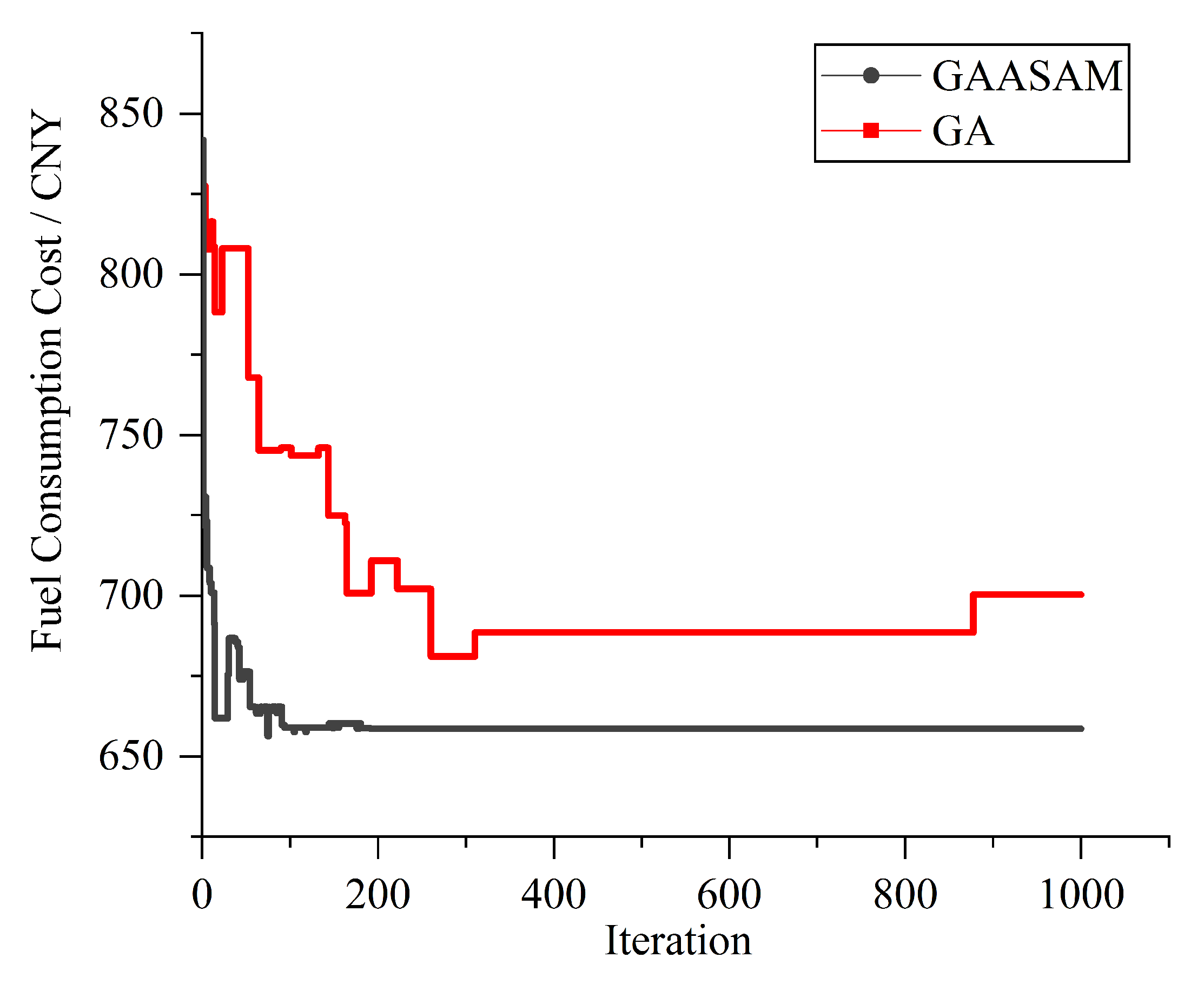
In order to verify the effectiveness of GAASAM, GAASAM is compared with the genetic algorithm (GA) for solving VRP proposed by Ombuki et al. [42] which is also suitable for solving the GFLHF-VRP. After the iterative evolution of the two algorithms, the total distribution cost, fuel consumption cost, refrigeration’s energy cost and carbon emission cost of the distribution route are obtained in the experiment, and the iterative curve is generated, as shown in Figure 3, Figure 4, Figure 5 and Figure 6. Then GAASAM is used to plan the route of this example, and the optimal distribution is obtained as shown in Figure 7. The comparison of the results of the optimal route given by two algorithms is obtained in

Table 5. Comparison of total distribution cost and environment-related costs between two algorithms.

Algorithms	Total Distribution Cost/CNY	Refrigeration’s Energy Cost/CNY	Fuel Consumption Cost/CNY	Carbon Emission Cost/CNY
GAASAM	2842.1	341.1	658.6	138.6
GA	2961.3	440.1	700.3	147.1

and

Table 6. Comparison of non-environment-related costs between two algorithms.

Algorithms	Fix Cost/CNY	Damage Cost/CNY	Overtime Penalty Cost/CNY
GAASAM	1500	170.1	33.7
GA	1500	150.7	23.2

.

As shown in Figure 3, Figure 4, Figure 5 and Figure 6, the iterative evolution curve of total distribution cost, fuel consumption cost, refrigeration’s energy consumption cost and carbon emission cost in the iterative evolution process are presented, when the number of iteration rounds reaches 200, each curve tends to be stable and reaches the lower value in GAASAM, and each curve is in an unstable state from 0 to 1000 iteration rounds in GA. Under the same experimental environment, the processing time for GAASAM is 107.8 s to propose the most optimal distribution; however, the processing time for GA is longer which is 112.9 s. As a result, the program running time of GAASAM is 4.52% shorter than that of GA. Through the comparison, GAASAM has faster convergence speed and can effectively avoid falling into the local optimal trap. The above iterative curves show that the proposed GAASAM effectively obtains the solution of GFLHF-VRP.

As shown in Table 5, compared with GA, using GAASAM effectively reduces 4.03% of the total distribution cost; and in environment-related costs, 5.95% of the the fuel cost, 22.52% of the refrigeration’s energy consumption cost and 5.78% of the carbon emission are reduced. The optimal distribution route proposed by GAASAM are with lower distribution cost, fuel consumption, energy consumption of refrigeration and carbon emission, which is more environment-friendly than the optimal distribution route proposed by GA.

As shown in Table 6, the non-environment-related costs obtained by using GAASAM are slightly higher compared to using GA. Comparing the experimental results of GAASAM and GA, the non-environment-related costs obtained by GAASAM, including damage costs and overtime penalty cost, have increased slightly. While the fixed cost remains the same, vehicle types of 1, 1, 1, 1, 1, 1, 2, 2, 3, 3, 3 are used in GAASAM’s optimal route, and vehicle types of 1, 1, 1, 1, 1, 2, 2, 2, 2, 3, 3 are used in GA’s optimal route. While the fixed costs under the two algorithms are the same, the differences in vehicle types and distribution route planning will affect the total vehicle distribution costs. In order to achieve the goal of green and the lowest total distribution cost, these three costs have been slightly increased by 1.79%.

Environmental protection issues for optimization of green fresh food logistics has been focused, so the total distribution cost comparison has been divided into two tables. Table 5 shows that GAASAM can significantly reduce the total distribution cost and three environmentally related costs when solving the GFLHF-VRP; Table 6 is the three basic costs in the basic vehicle routing problem for fresh food logistics. According to Table 5 and Table 6, GAASAM can solve the GFLHF-VRP effectively.

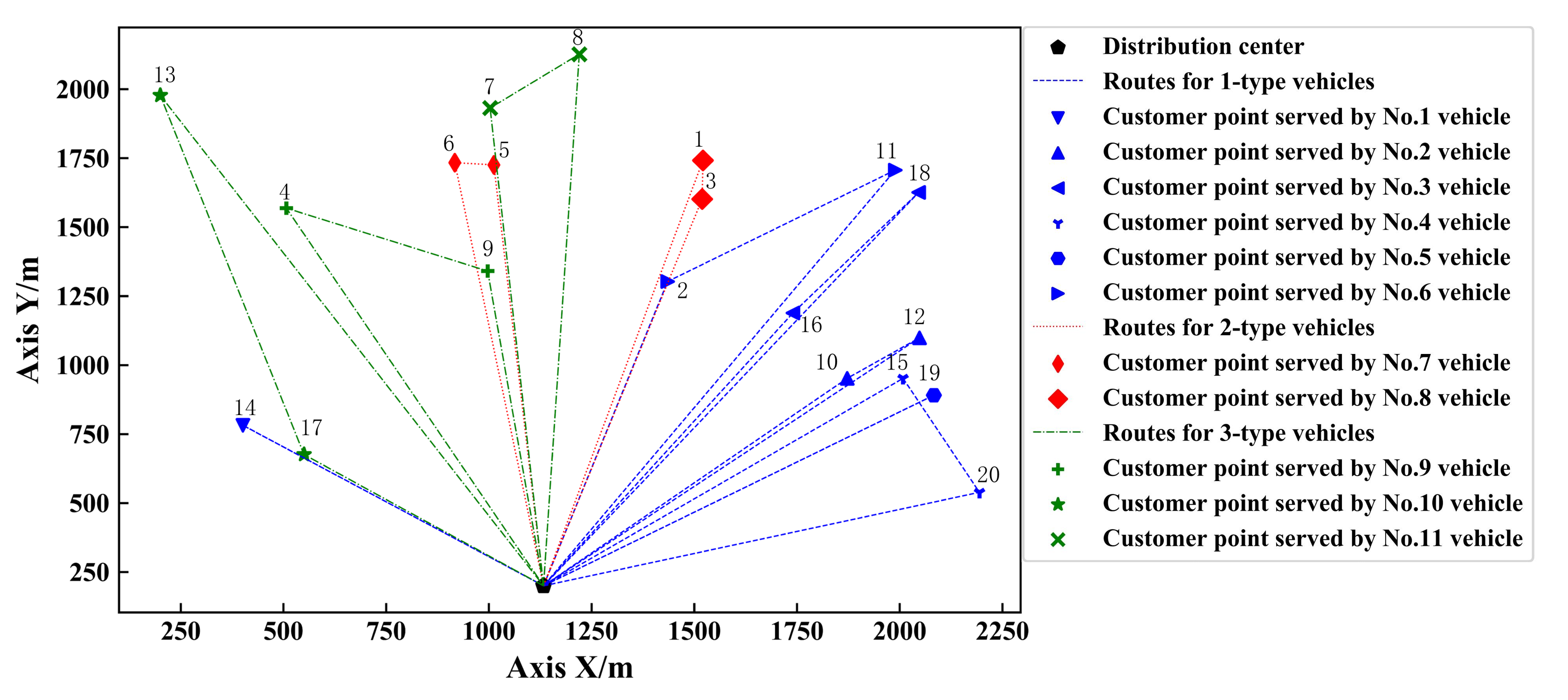
The optimal vehicle distribution route obtained by GAASAM is shown in Figure 7. Total of 11 vehicles are dispatched for this distribution task, with types of 1, 1, 1, 1, 1, 1, 2, 2, 3, 3, 3, respectively. The vehicle is numbered from 1 to 11 in turn. Each vehicle starts from the distribution center according to its own distribution route, serves its customer points in turn, and then returns to the distribution center, with distribution routes of 0-14-0, 0-10-12-0, 0-16-18-0, 0-20-15-0, 0-2-11-0, 0-19-0, 0-5-6-0 0-1-3-0, 0-9-4-0, 0-17-13-0, 0-7-8-0, i.e., 0-7-8-0 represents that the vehicle of type 3 and number 11 starts from the distribution center to serve the customer point 7, customer point 8 and then returns to the distribution center. Fresh logistics companies can use GAASAM to get a vehicle distribution routes planning similar to Figure 7, which has the lowest total distribution cost and protects the environment.

6. Discussion

In recent years, automobile fuel consumption, energy consumption and carbon emissions have a certain degree of harm to the environment, and issues related to the greenhouse effect and pollutant emissions have continued increasing. At the same time, with the improvement of quality of life, people’s demand for fresh products is increasing, and fresh food logistics has also developed unprecedentedly. However, fresh food logistics is an industry with high energy consumption and high pollution. Utilizing technological means to achieve the reduction of energy consumption and pollutant emissions during the distribution of fresh logistics also have a positive effect on environment. Many scholars have focused on the VRP models in various scenarios. Among them, in order to reduce the emission of pollutants from distribution vehicles, a number of researchers have begun to study the issues related to Green Vehicle Route problem (G-VRP). At the same time, there are also some researches on the VRP model for fresh food logistics and cold chain logistics. The VRP model for fresh food logistics mainly integrates as many costs as possible, such as transportation costs, fixed costs, and timeout penalty costs, damage costs of goods, carbon emission costs, etc. However, few people focused on the research on the environment-friendly distribution of fresh food logistics and proposed the related VRP model. Therefore, the GFLHF-VRP model has been established, which not only integrates the cost items in the fresh logistics currently known, but also introduces the concept of multi-type of vehicle and the fuel consumption cost, refrigeration’s energy cost and the carbon emission cost.

The vehicle route problem belongs to NP-hard problem that usually needs to be solved by using a heuristic algorithm to obtain the optimal results. Among them, commonly used algorithms include genetic algorithm, simulated annealing algorithm, ant colony algorithm, particle swarm algorithm, tabu search algorithm, etc. In GFLHF-VRP model, there are six kinds of costs and the calculation process of costs is more complicated. Therefore, an innovative GAASAM is designed and upgraded from GA, in which the simulated annealing algorithm and adaptive operation are mainly introduced. In GAASAM, the simulated annealing algorithm is used to perform the mutation operation to fully realize the neighborhood solution search in the evolution process, and an adaptive operation is introduced to set the parameters of the simulated annealing algorithm. Then the experimental results show that the proposed GAASAM effectively plan the optimal route for GFLHF-VRP model, and jump out of the local optimal trap during the iterative evolution process; furthermore, it also effectively reduce the costs related to the environment in green fresh food logistics. The optimal vehicle distribution route proposed by GAASAM effectively reduce the total distribution cost by 3.86%, fuel consumption cost by 21.43%, refrigeration energy consumption cost by 5.96% and carbon emission cost by 5.78%, compared with that proposed by GA; although the non-environment-related costs are increased slightly by 1.79%, they are insignificant compared to the reduction in environmental-related costs and in total distribution costs.

From the practical point of view, GAASAM is proposed in this article for the fresh food logistics enterprise, used to get the optimal route of its fresh food logistics scenario and obtain the optimal path for its reference which have less distribution costs, reduce the cost of the enterprise and the pollution to the environment, so that the enterprise is better on taking the social responsibility of protecting the environment. Through research on GFLHF-VRP and GAASAM, some managerial insights are summarized as follows:

• More distribution vehicles that are suitable for fresh logistics with lower carbon emissions, lower fuel consumption and battery that can efficiently supply the energy for refrigerators should be used in fresh food logistics.
• Fresh food logistics enterprises should analyze their own logistics business with actual data to establish a complete mathematical model where experimental factors should be focused, and solve the model’s vehicle route problems through scientific algorithms; e.g., those enterprises can utilize the GFLHF-VRP model and GAASAM proposed in this paper to establish a greener and environmentally friendly distribution route for their own logistics business.
• The government should introduce concepts for fresh logistics companies to reduce carbon emissions, fuel consumption, and power consumption in the distribution process, and increase their environmental responsibility.

7. Conclusions

In this paper, the concept of environmental protection is introduced for fresh food logistics, and a GFLHF-VRP model is established in accordance with the actual application scenario. At the same time, an improved genetic algorithm called Genetic Algorithm with Adaptive Simulated Annealing Mutation (GAASAM) is proposed, which takes the fixed cost, fuel consumption cost, refrigeration’s energy consumption cost, carbon emission cost, damage cost and overtime penalty cost into account. The comparison between GAASAM and GA through experiments shows that GAASAM has a faster convergence speed and effectively avoids falling into the local optimal trap. Furthermore, the results show that the total distribution cost, fuel consumption, refrigeration’s energy consumption, carbon emissions of the optimal distribution route proposed by GAASAM are lower than those of the optimal distribution route proposed by GA. The effectiveness of GAASAM is verified through experiments; it has been proved that GAASAM can achieve the goal of reducing total distribution cost, saving energy and reducing carbon emissions, and can provide a green vehicle route for GFLHF-VRP model. The GFLHF-VRP model and GAASAM proposed in this paper have certain practical significance and can be used as a reference for related fresh logistics companies to planning the optimal vehicle distribution route which has lower distribution cost and is more environment-friendly.

These insights enable fresh logistics enterprises to reduce the total cost of distribution as much as possible when protecting the environment. This paper focuses on the cost of green distribution, and the customer satisfaction factor may be an interesting entry point of in-depth study.

References

- Wang, X. Changes in CO2 Emissions induced by agricultural inputs in China over 1991–2014. Sustainability 2016, 8, 414. [Google Scholar] [CrossRef] [Green Version]
- Gregg, J.S.; Andres, R.J.; Marland, G. China: Emissions pattern of the world leader in CO2 emissions from fossil fuel consumption and cement production. Geophys. Res. Lett. 2008, 35. [Google Scholar] [CrossRef]
- Zhang, J.; Zhao, Y.; Xue, W.; Jin, L. Vehicle routing problem with fuel consumption and carbon emission. Int. J. Prod. Econ. 2015, 170, 234–242. [Google Scholar] [CrossRef]
- Montanari, R. Cold chain tracking: A managerial perspective. Trends Food Sci. Technol. 2008, 19, 425–431. [Google Scholar] [CrossRef]
- Mercier, S.; Villeneuve, S.; Mondor, M.; Uysal, I. Time–temperature management along the food cold chain: A review of recent developments. Compr. Rev. Food Sci. Food Saf. 2017, 16, 647–667. [Google Scholar] [CrossRef]
- Kuo, J.C.; Chen, M.C. Developing an advanced multi-temperature joint distribution system for the food cold chain. Food Control 2010, 21, 559–566. [Google Scholar] [CrossRef]
- Chen, J.; Gui, P.; Ding, T.; Na, S.; Zhou, Y. Optimization of Transportation Routing Problem for Fresh Food by Improved Ant Colony Algorithm Based on Tabu Search. Sustainability 2019, 11, 6584. [Google Scholar] [CrossRef] [Green Version]
- James, S.J.; James, C. The food cold-chain and climate change. Food Res. Int. 2010, 43, 1944–1956. [Google Scholar] [CrossRef]
- Wang, S.; Tao, F.; Shi, Y.; Wen, H. Optimization of vehicle routing problem with time windows for cold chain logistics based on carbon tax. Sustainability 2017, 9, 694. [Google Scholar] [CrossRef] [Green Version]
- Qiao, J. Research on optimizing the distribution route of food cold chain logistics based on modern biotechnology. AIP Conf. Proc. AIP Publ. 2019, 2110, 020070. [Google Scholar]
- Strandhagen, J.O.; Vallandingham, L.R.; Fragapane, G.; Strandhagen, J.W.; Stangeland, A.B.H.; Sharma, N. Logistics 4.0 and emerging sustainable business models. Adv. Manuf. 2017, 5, 359–369. [Google Scholar] [CrossRef]
- Facchini, F.; Oleśków-Szłapka, J.; Ranieri, L.; Urbinati, A. A Maturity Model for Logistics 4.0: An Empirical Analysis and a Roadmap for Future Research. Sustainability 2019, 12, 86. [Google Scholar] [CrossRef] [Green Version]
- Boenzi, F.; Digiesi, S.; Facchini, F.; Mossa, G. Greening Activities in Warehouses: A Model for Identifying Sustainable Strategies in Material Handling. Ann. DAAAM Proc. 2015, 26, 980–988. [Google Scholar]
- Facchini, F.; Pascale, G.D.; Faccilongo, N. Pallet picking strategy in food collecting center. Appl. Sci. 2018, 8, 1503. [Google Scholar] [CrossRef] [Green Version]
- Kuo, Y.; Wang, C.C. Optimizing the VRP by minimizing fuel consumption. Manag. Environ. Q. Int. J. 2011, 22, 440–450. [Google Scholar] [CrossRef]
- Bektaş, T.; Laporte, G. The pollution-routing problem. Transp. Res. Part B Methodol. 2011, 45, 1232–1250. [Google Scholar] [CrossRef]
- Erdoğan, S.; Miller-Hooks, E. A green vehicle routing problem. Transp. Res. Part E: Logist. Transp. Rev. 2012, 48, 100–114. [Google Scholar] [CrossRef]
- Koç, Ç.; Karaoglan, I. The green vehicle routing problem: A heuristic based exact solution approach. Appl. Soft Comput. 2016, 39, 154–164. [Google Scholar] [CrossRef]
- Xiao, Y.; Zhao, Q.; Kaku, I.; Xu, Y. Development of a fuel consumption optimization model for the capacitated vehicle routing problem. Comput. Oper. Res. 2012, 39, 1419–1431. [Google Scholar] [CrossRef]
- Kwon, Y.J.; Choi, Y.J.; Lee, D.H. Heterogeneous fixed fleet vehicle routing considering carbon emission. Transp. Res. Part D Transp. Environ. 2013, 23, 81–89. [Google Scholar] [CrossRef]
- Bortolini, M.; Faccio, M.; Ferrari, E.; Gamberi, M.; Pilati, F. Fresh food sustainable distribution: Cost, delivery time and carbon footprint three-objective optimization. J. Food Eng. 2016, 174, 56–67. [Google Scholar] [CrossRef]
- Niu, Y.; Yang, Z.; Chen, P.; Xiao, J. Optimizing the green open vehicle routing problem with time windows by minimizing comprehensive routing cost. J. Clean. Prod. 2018, 171, 962–971. [Google Scholar] [CrossRef]
- Naderipour, M.; Alinaghian, M. Measurement, evaluation and minimization of CO2, NOx, and CO emissions in the open time dependent vehicle routing problem. Measurement 2016, 90, 443–452. [Google Scholar] [CrossRef] [Green Version]
- Hsu, C.I.; Hung, S.F.; Li, H.C. Vehicle routing problem with time-windows for perishable food delivery. J. Food Eng. 2007, 80, 465–475. [Google Scholar] [CrossRef]
- Osvald, A.; Stirn, L.Z. A vehicle routing algorithm for the distribution of fresh vegetables and similar perishable food. J. Food Eng. 2008, 85, 285–295. [Google Scholar] [CrossRef]
- Wu, Y.; Meng, Z.B.; Peng, M. The Research on the Optimization of Transportation Routing for Fresh Food by Improved Genetic Algorithm. Appl. Mech. Mater. Trans. Tech. Publ. 2012, 178, 1790–1796. [Google Scholar] [CrossRef]
- Amorim, P.; Parragh, S.N.; Sperandio, F.; Almada-Lobo, B. A rich vehicle routing problem dealing with perishable food: A case study. Top 2014, 22, 489–508. [Google Scholar] [CrossRef]
- Li, Y.; Chu, F.; Yang, Z.; Calvo, R.W. A production inventory routing planning for perishable food with quality consideration. IFAC-PapersOnLine 2016, 49, 407–412. [Google Scholar] [CrossRef]
- Wang, S.; Tao, F.; Shi, Y. Optimization of location–routing problem for cold chain logistics considering carbon footprint. Int. J. Environ. Res. 2018, 15, 86. [Google Scholar] [CrossRef] [Green Version]
- Shukla, M.; Jharkharia, S. Artificial Immune System-based algorithm for vehicle routing problem with time window constraint for the delivery of agri-fresh produce. J. Decis. Syst. 2013, 22, 224–247. [Google Scholar] [CrossRef]
- Wang, X.; Wang, M.; Ruan, J.; Zhan, H. The multi-objective optimization for perishable food distribution route considering temporal-spatial distance. Procedia Comput. Sci. 2016, 96, 1211–1220. [Google Scholar] [CrossRef] [Green Version]
- Chen, H.K.; Hsueh, C.F.; Chang, M.S. Production scheduling and vehicle routing with time windows for perishable food products. Comput. Oper. Res. 2009, 36, 2311–2319. [Google Scholar] [CrossRef]
- Norouzi, N.; Sadegh-Amalnick, M.; Tavakkoli-Moghaddam, R. Modified particle swarm optimization in a time-dependent vehicle routing problem: Minimizing fuel consumption. Optim. Lett. 2017, 11, 121–134. [Google Scholar] [CrossRef]
- Park, J.B.; Park, Y.M.; Won, J.R.; Lee, K.Y. An improved genetic algorithm for generation expansion planning. IEEE Trans. Power Syst. 2000, 15, 916–922. [Google Scholar] [CrossRef] [Green Version]
- Andre, J.; Siarry, P.; Dognon, T. An improvement of the standard genetic algorithm fighting premature convergence in continuous optimization. Adv. Eng. Softw. 2001, 32, 49–60. [Google Scholar] [CrossRef]
- Pishvaee, M.S.; Kianfar, K.; Karimi, B. Reverse logistics network design using simulated annealing. Int. J. Adv. Manuf. Technol. 2010, 47, 269–281. [Google Scholar] [CrossRef]
- Lipowski, A.; Lipowska, D. Roulette-wheel selection via stochastic acceptance. Phys. A 2012, 391, 2193–2196. [Google Scholar] [CrossRef] [Green Version]
- Goldberg, D.E.; Lingle, R. Alleles, loci, and the traveling salesman problem. In Proceedings of the Internationa l Conference on Genetic Algorithms and Their Applications; Lawrence Erlbaum: Hillsdale, NJ, USA, 1985; pp. 154–159. [Google Scholar]
- Santos, J.; Ferreira, A.; Flintsch, G. An adaptive hybrid genetic algorithm for pavement management. Int. J. Pavement Eng. 2019, 20, 266–286. [Google Scholar] [CrossRef]
- Wang, C.; Lin, J.; Lin, M.; Zhong, Y. Evolutionary harmony search algorithm with metropolis acceptance criterion for travelling salesman problem. Int. J. Wirel. Mob. Comput. 2016, 10, 166–173. [Google Scholar] [CrossRef]
- Tavakkoli-Moghaddam, R.; Safaei, N.; Gholipour, Y. A hybrid simulated annealing for capacitated vehicle routing problems with the independent route length. Appl. Math. Comput. 2006, 176, 445–454. [Google Scholar] [CrossRef]
- Ombuki, B.; Ross, B.J.; Hanshar, F. Multi-objective genetic algorithms for vehicle routing problem with time windows. Appl. Intell. 2006, 24, 17–30. [Google Scholar] [CrossRef]
Figure 1.
Example of individual gene sequence.
Figure 2.
The flowchart of genetic algorithm of adaptive simulated annealing mutation (GAASAM).
Figure 3.
Comparison of total distribution cost between two algorithms.
Figure 4.
Comparison of fuel consumption cost between two algorithms.
Figure 5.
Comparison of refrigeration’s energy consumption cost between two algorithms.
Figure 6.
Comparison of carbon emission cost between two algorithms.
Figure 7.
Optimal vehicle distribution route graph of GAASAM.