Solving the Multi-Depot Green Vehicle Routing Problem by a Hybrid Evolutionary Algorithm

1
School of Business Administration, Southwestern University of Finance and Economics, Chengdu 610074, China
2
College of Management, Sichuan Agricultural University, Chengdu 610074, China
3
Department of Finance, Wenzhou Business College, Wenzhou 325035, China
*
Author to whom correspondence should be addressed.
Sustainability 2020, 12(5), 2127; https://0-doi-org.brum.beds.ac.uk/10.3390/su12052127
Submission received: 31 January 2020
/
Revised: 1 March 2020
/
Accepted: 5 March 2020
/
Published: 9 March 2020
(This article belongs to the Section Sustainable Transportation)
Abstract
:The growing concerns about human pollution has motivated practitioners and researchers to focus on the environmental and social impacts of logistics and supply chains. In this paper, we consider the environmental impact of carbon dioxide emission on a vehicle routing problem with multiple depots. We present a hybrid evolutionary algorithm (HEA) to tackle it by combining a variable neighborhood search and an evolutionary algorithm. The proposed hybrid evolutionary algorithm includes several distinct features such as multiple neighborhood operators, a route-based crossover operator, and a distance- and quality-based population updating strategy. The results from our numerical experiments confirm the effectiveness and superiority of the proposed HEA in comparison with the best-performing methods in the literature and the public exact optimization solver CPLEX. Furthermore, an important aspect of the HEA is studied to assess its effect on the performance of the HEA.
1. Introduction
During the past decades, the acceleration of energy consumption and environmental pollution have become worldwide concerns. In particular, greenhouse gas emissions and the resulting climate change may have caused more and more disasters worldwide. Consequently, many countries and regions are making huge efforts to reduce greenhouse gas emissions [1]. Meanwhile, consumer pressures and environmental regulations have incentivized many companies to incorporate the environmental considerations into their logistics and supply chain management. As a result, many logistics providers have endeavored to integrate environmental management with their logistics. This has increased the complexity in logistics optimization problems partly because of the potential conflicts between economic and ecological concerns [2].
The environmentally sensitive logistics system requires designing sustainable distribution networks with less negative impact on the environment and the ecology. There are many factors related to green transportation, such as alternative fuels, electric vehicles, and environmental protection infrastructure. In addition, an explicit consideration is given to reducing CO2 levels through better operating plans. Particularly, the uncertainty about the carbon emissions and mitigation design have obtained lots of attention and research in recent years [3,4] since it has become a huge issue in real life. In order to better study the impact of carbon emissions, in this study we consider and address the carbon emissions as an economic factor.
The vehicle routing problem (VRP) and its related variants have become the subject of lots of research in the literature, which is mainly due to the additional constraints and increasing number of targets caused by realistic problems. For the classic vehicle routing problem, the focus of research is based on the economic part of vehicle routing on companies that provide distribution services. Given the increasing global concern over environmental problems, VRP problems have recently begun to include “green” issues such as alternative fuels and pollution. In particular, multiple objectives and more operational constraints have been incorporated in vehicle routing models for green logistics, which lead to more difficult and more complex optimization problems. As a matter of fact, green logistics have been extensively studied in the literature [5,6] focusing on the environmental effects of different distribution strategies, managing waste disposal, reducing the energy consumption, and adopting the delivery service of the unmanned aerial vehicles. In addition, many new models of transport have recently been presented to improve fuel efficiency and reduce adverse environmental impacts, such as the latest survey on green freight. [7,8].
In order to enrich the research and provide effective ideas and competitive methods for solving the VRP variant regarding these sustainable transportation issues, in this study we attempt to consider a VRP variant with a realistic multi-depot scenario by harmonizing the environmental and economic costs and determining the assignment of customers to depots.
1.1. Literature Review
The literature on green vehicle routing problems mainly considered three factors: energy consumption, pollution reduction, and waste management. In the following paragraphs, we will review the related papers in terms of the three aspects.
Palmer [9] was the first to study the environmental issues in the VRPs. Unlike the previous studies that investigated the environmental costs based on the total distance or duration, the authors considered other issues such as road terrain, vehicle speed, and traffic congestion to generate a matrix of CO2 gas emissions. Their computation results showed that, compared with the distance minimization model and the duration minimization model, the proposed CO2 minimization model reduced the CO2 gas emissions.
Later on, Kara et al. [10] proposed a mathematical formula called the energy-minimizing vehicle routing problem (EMVRP), whose purpose was to minimize the sum of the product of the load and distance for each arc. A similar approach was presented to reduce fuel consumption or CO2 emissions [11,12]. Specifically, Demir et al. [11] made numerical comparisons of several freight vehicle emission models in consideration of their performance in field studies. They demonstrated that reducing greenhouse gas emissions in freight required the use of appropriate emission models in the planning process.
The pollution routing problem (PRP) is a class of green vehicle routing problems. Bektas and Laporte [13] first proposed the PRP that aimed to minimize both environmental and operational costs, taking the greenhouse emissions, fuel, and travel times into account. The authors made a computational analysis to achieve the balance between each variation and speed constraints on the energy, distance, and costs. After that, Demir et al. [14] presented an adaptive large neighborhood search (ALNS) for the PRP problem with the time-window constraints. As a further extension, Demir et al. [15] considered a bi-objective PRP, in which both objectives, namely the minimization of fuel consumption and the minimization of driving time, were conflicting and tackled, respectively. They solved the bi-objective PRP by combining the ALNS method with four a posteriori methods. Their experimental results showed the presented hybrid approach can solve PRP instances with up to 100 nodes. Gajanand and Narendran [16] developed a multiple-route VRP to assess alternative routes between benchmarks and addressed the issue to minimize fuel consumption. Tiwari and Chang [17] employed the distance-based method to calculate the CO2 emissions, where vehicle load was tackled as an important factor. They generated different clusters for each city they traveled to using different trucks and applied a block reorganization method to the GVRP problem, where each cluster denoted a block. Suzuki [18] considered the minimization of the emissions from vehicles and fuel consumption. For solving it, they proposed a solution method which employed the mechanism of efficient frontier to exploit the promising area in the solution space.
Considering the importance of multiple depots and maximum capacity constraints in practical scenarios, Jabir et al. [19] integrated emissions and economic costs for a capacitated multi-depot GVRP. An integer linear programming model was formulated to solve a lot of small-scale instances by employing the optimization solver Lingo. In addition, they employed an ant colony optimization (ACO) algorithm to tackle small-scale as well as large-scale problems within a reasonable amount of time.
1.2. Motivations and Contributions
The key point to design an effective heuristic method relies on an appropriate trade-off between search intensification and diversification. Hybrid evolutionary algorithms have shown great performance for solving many optimization problems, such as the job shop scheduling problem [20], cutwidth minimization problem [21], and course timetabling problem [22]. To the best of our knowledge, there have been no previous papers using evolutionary algorithms to solve the MDGVRP. Additionally, there are few neighborhood operators in the previous studies in the literature. To help tackle this computationally challenging problem in MDGVRP, in this study we propose a hybrid evolutionary algorithm (HEA) to achieve a better trade-off between the exploitation and exploration in the solution space.
Generally, the HEA algorithm [20,23] is a well-known variant algorithm of the evolutionary algorithm that combines the intensification strength of local optimization and the diversification power of the evolutionary algorithm. The proposed HEA can further be employed to solve the single-depot GVRP, since it can be considered as a special issue of multi-depot GVRP when the number of depots equals 1.
The main contributions in our study are summarized as follows:
- We first present a hybrid evolutionary algorithm by incorporating a variable neighborhood search method into the framework of an evolutionary algorithm to solve MDGVRP;
- We propose several dedicated neighborhood operators extending the previous search operators in ACO method [19] for search intensification, and the route-based crossover operator for search diversification;
- We present a distance- and quality-based replacement strategy to update the population;
- Extensive experimental results demonstrate the proposed HEA method can obtain a better trade-off in terms of the computational efficiency and solution quality in comparison with the previous ACO method in literature;
- These ideas of the proposed combined evolutionary-based framework and the variable neighborhood search suitable for solving MDGVRP are general and can be employed as a reference for other related GVRPS.
The sections of the paper are organized as follows. Section 2 gives the MDGVRP and its mathematic model. Section 3 proposes the hybrid evolutionary algorithm. Section 4 gives the experimental protocols and parameter setting and reports the computational results and performance comparisons with the best-performing heuristics in the literature and the exact optimization solver CPLEX. The effectiveness of the route-based crossover operator, a key component in the proposed algorithm, is evaluated in Section 5. Section 6 shows the advantages and limitations of the proposed HEA method. At last, conclusion comments and future potential research areas are presented in Section 7.
2. Problem Description and Mathematic Model
In line with [19], we assume that the vehicles and depots were capacitated with maximum limit constraint. Additionally, we considered similar vehicles with the same speed, capacity, and emissions characteristics. There were environmental and economic costs related with the distribution plan. To be specific, there were two components, i.e., the variable cost and fixed cost, in the economic part. The fixed cost is usually associated with one-time expenditures, such as the rent, the insurance expenses, and other maintenance costs of vehicles. The variable cost considers the expenditure on fuel consumption. Additionally, the environmental costs in this study evaluated the monetary values of CO2 emissions in the route of vehicle.
We followed the mathematical model from Jabir et al. [19]. The symbols and their definitions for MDGVRP are given in Table 1. The mathematical model for MDGVRP is given as follows:
Model constraints:
The objective function presented in Equation (1) seeks to minimize the total cost. Constraint (2) ensures the transportation from a depot to another depot is not permitted. Constraint (3) avoids that the source and the destination are the same. Constraint (4) ensures that a vehicle only can serve one customer each time. Constraint (5) ensures that a single link arrives at and departs from the customer routine. Constraint (6) ensures that the number of outbound links from a depot should be equal to the number of inbound links. Constraint (7) ensures that each vehicle should depart from a depot. Constraint (8) ensures that an empty vehicle returns to a depot. Constraint (9) ensures that the lower bound of the vehicle load in which the vehicle should satisfy the requirement of the destination node as the minimum value. Constraint (10) ensures the upper bound of vehicle load, where the difference between the maximum capacity of vehicle and the requirement of customer node when a vehicle departs from vertex to vertex . Constraint (11) ensures the vehicle load flow balance. Constraint (12) ensures that the depot capacity cannot exceed the maximum capacity upper bound. Constraint (13) illustrates the sub-tour elimination constraints. Constraint (14) guarantees the binary integrality.
3. A Hybrid Evolutionary Algorithm for MDGVRP
The hybrid evolutionary algorithm proposed in our study was a population-based approach that included several important phases: initial population procedure, variable neighborhood search phase, crossover operator, and population updating mechanism. The initial population procedure aimed to generate diversified solutions with good quality. The variable neighborhood search phase was able to effectively obtain the local optima for search intensification. The route-based crossover operator and distance-and-quality population updating strategy can enhance the search diversification of the proposed method. We present the general framework of HEA and its ingredients in the following subsection.
3.1. The Main Framework of HEA for MDGVRP
The proposed HEA algorithm follows the general scheme of evolutionary algorithms and consists of three major components: the population initialization phase to produce a random initial population, the variable neighborhood search (VNS) procedure to improve the incumbent solution, and the route-based crossover operator to generate an offspring. The algorithm progresses through a number of iterative cycles involving VNS and crossover operations. A pictorial representation of one cycle of the algorithmic framework is given in Algorithm 1.
3.2. Initial Population Phase
The initial population procedure aims to generate diversified solutions with good quality. Specifically, in order to obtain an initial solution S, which consists of several routes, we present a random greedy construction method inspired from the iterated greedy construction procedure in [24] given as follows:
- Step 1: Each route of S is initialized by generating a randomly selected depot Rc as the first node and a randomly customer node as the second node.
Algorithm 1. The framework of the proposed HEA for MDGVRP. 1: Input: Problem instance , size of population
2: Output: Best found solution
3: , …,
4: for {1, …, } do
5:
6: end for
7: while the maximum running time is not met do
8: Choose two random individuals and from population P
9:
10:
11: if then
12: ,
13: end if
14:
15: end while
16: return - Step 2: As for each route, a nearest node to the last node of the current route Rc is iteratively selected and inserted into the current route Rc until the current vehicle cannot serve the remaining customers.
The initial construction procedure is iteratively executed p times to generate several random and initial solutions. Additionally, each solution can be further optimized with a dedicated variable neighborhood search phase. The initialization phase generates an initial population consisting of several solutions with relatively good quality.
3.3. Variable Neighborhood Search Procedure
The local refinement procedure is a very important component in the method to obtain the local optima. In this study, the proposed HEA employs variable neighborhood search (VNS) as the local refinement method to improve the initial solution and offspring solutions in population. The key ingredients of a VNS-based approach are several neighborhood operators and shaking phase.
Neighborhood Structure
The proposed six neighborhood operators employed in the VNS procedure can be given as follows:
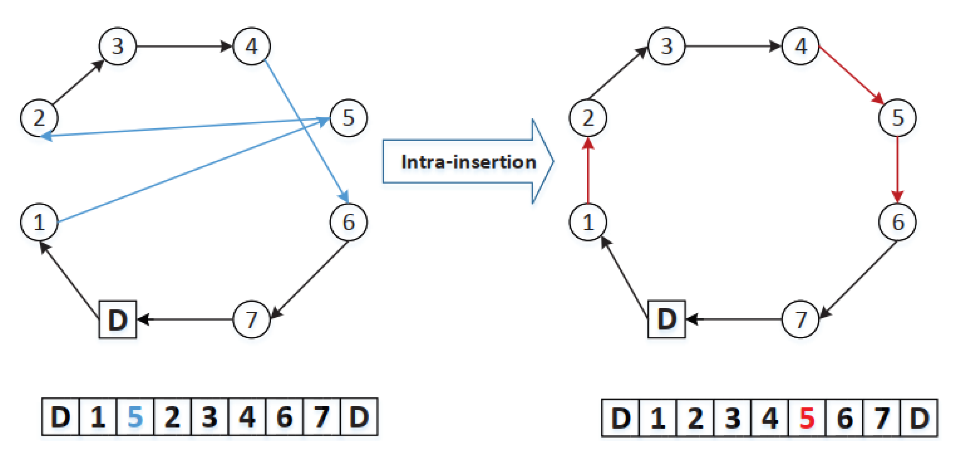
- Intra-insertion ( ): The operator chooses a customer in a route and relocates it in the current route (Figure 1);
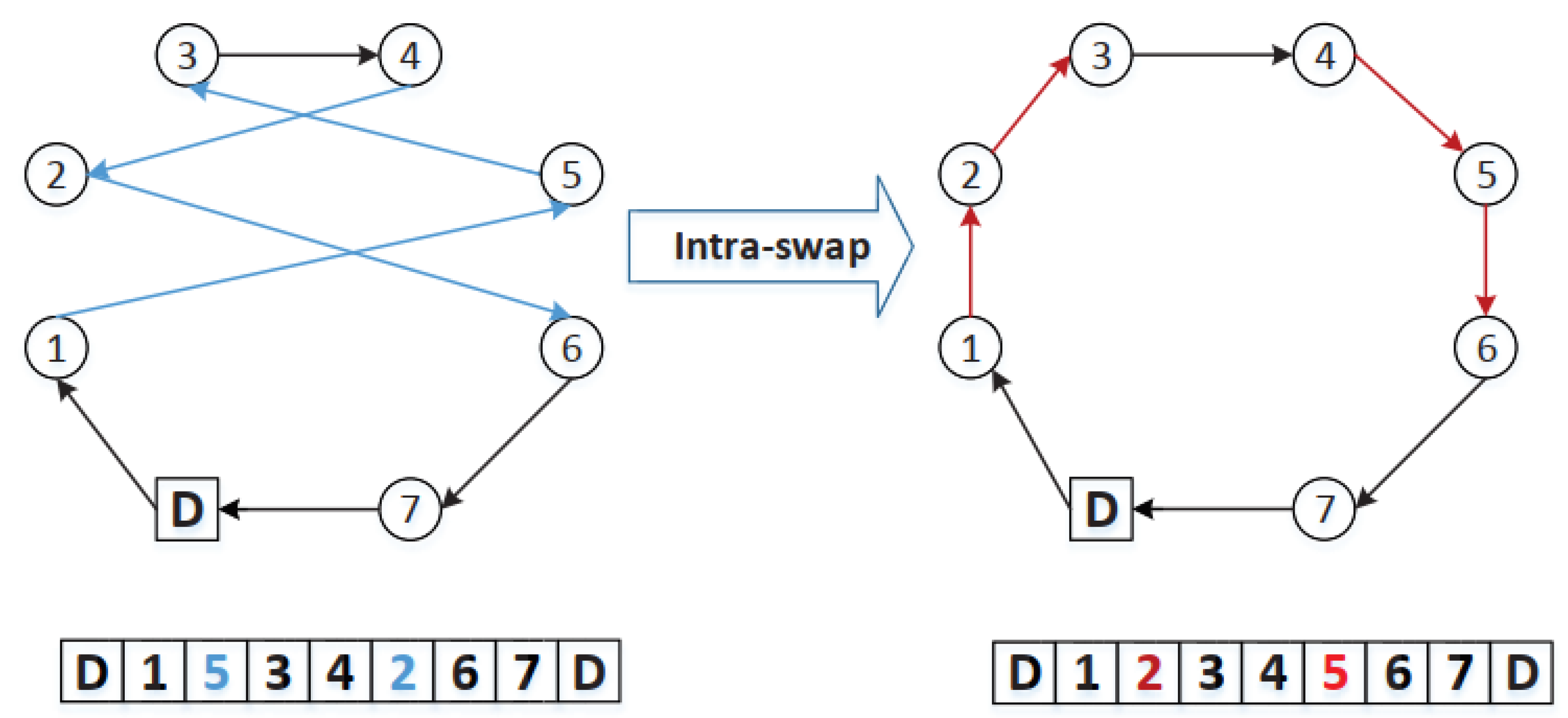
- Intra-swap (): The operator exchanges the positions of two customers in the same route (Figure 2);
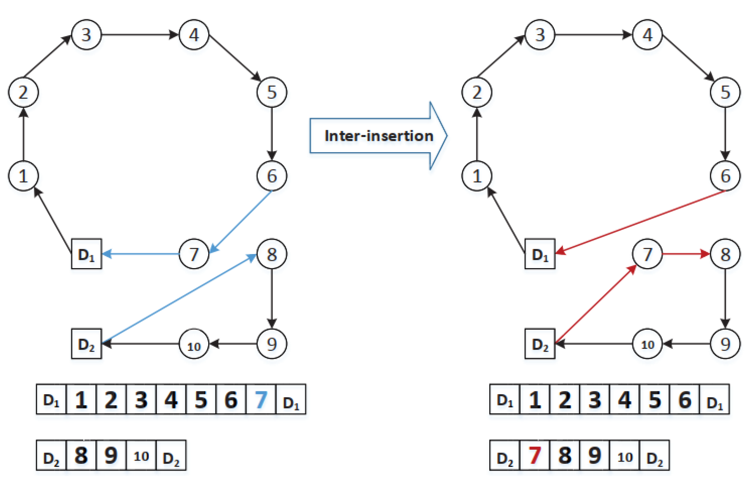
- Inter-insertion (): Unlike the intra-insertion operator (), the operator chooses a customer node from a given route and relocates it in another different route (Figure 3);
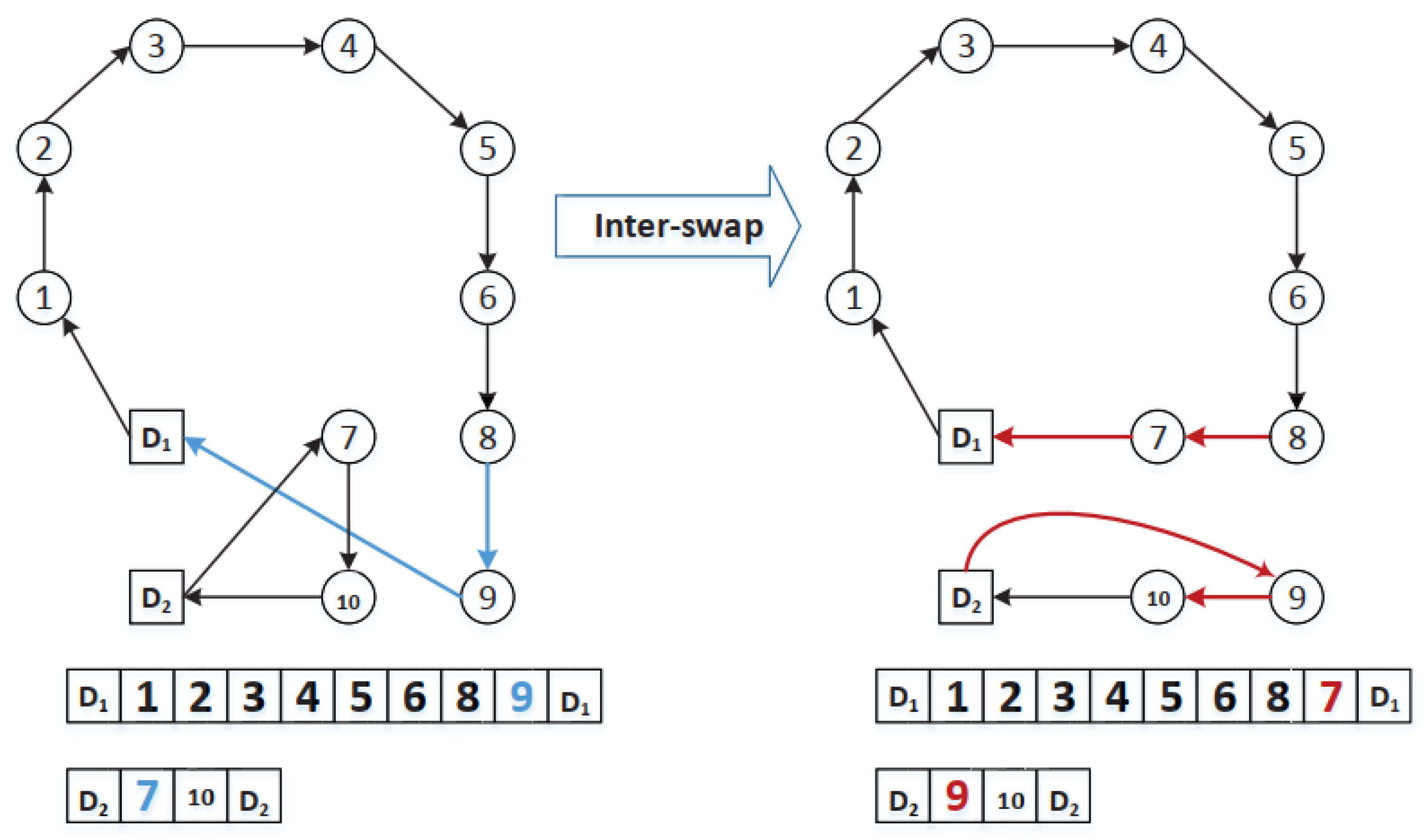
- Inter-swap (): Unlike the intra-swap operator (), the operator exchanges the positions of two customers in different routes (Figure 4);
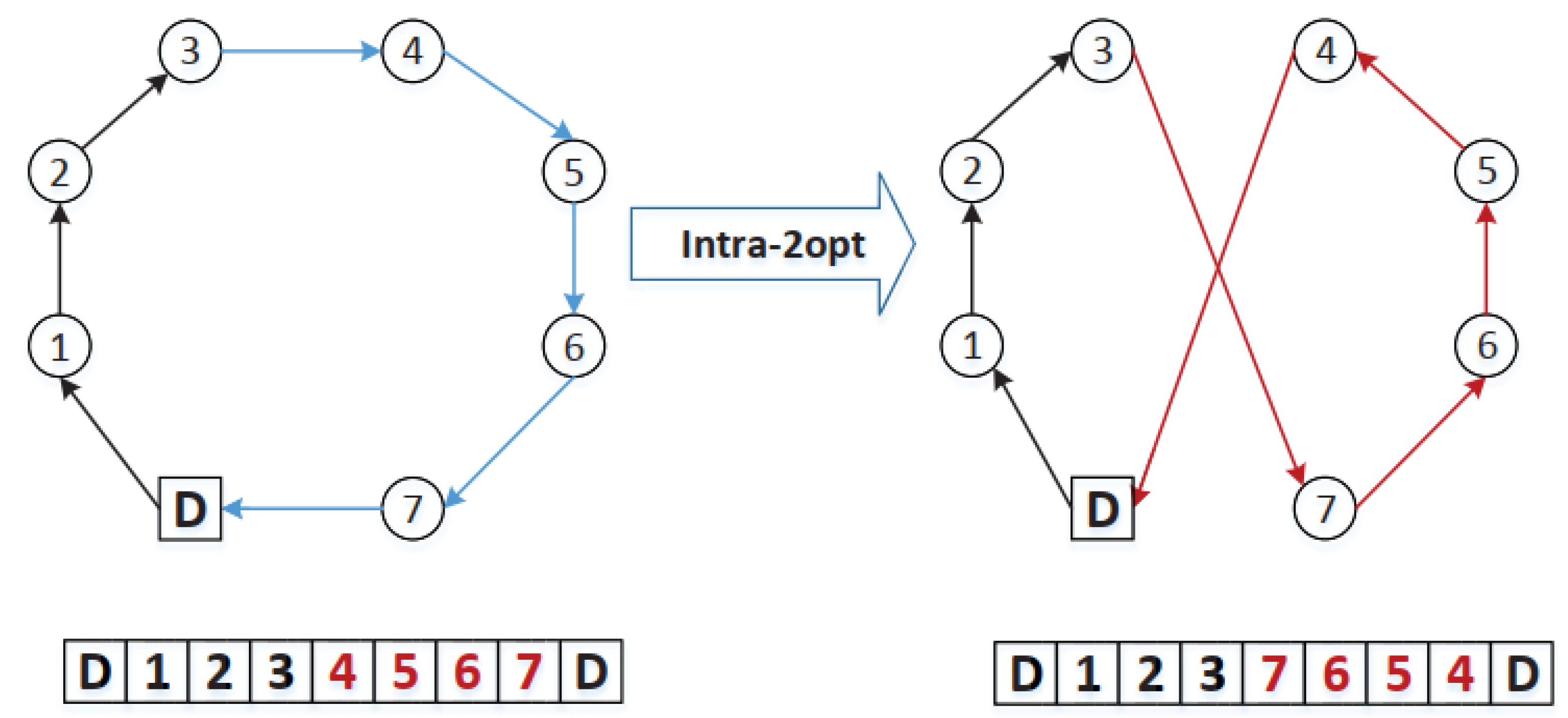
- Intra-2opt (): The operator deletes two non-adjacent edges, reverses the intermediate customer nodes in the route, and relinks the route by adding two new edges (Figure 5);
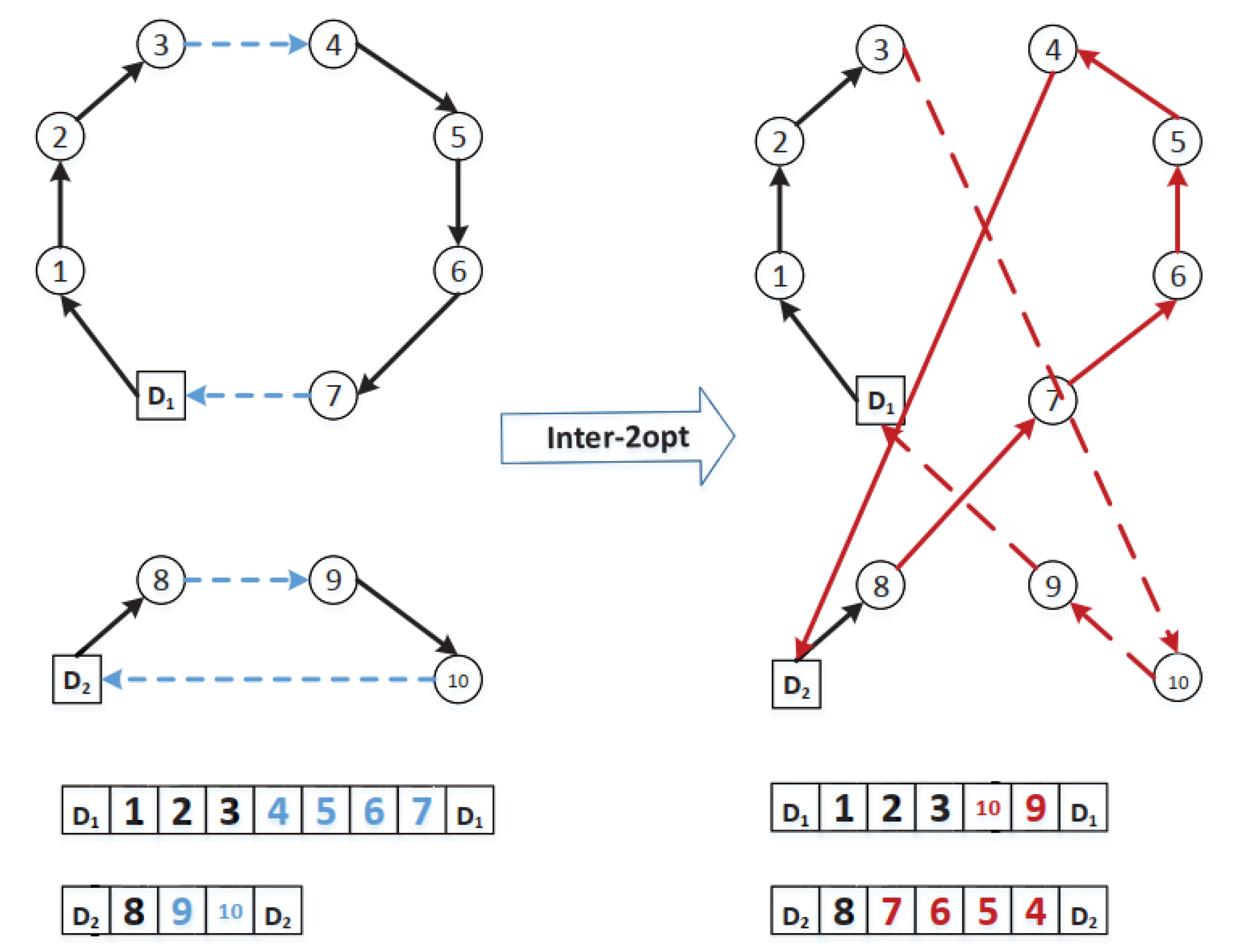
- Inter-2opt (): The operator eliminates two edges in different routes. Then, each route is cut into two parts, respectively. After that, it reverses two middle customer nodes in two routes and relinks each first part of a route with the last part of the other route to obtain two new routes (Figure 6).
| Algorithm 2. Variable neighborhood search |
| 1: Input: Initial solution ; maximum iterations without improvement 2: Output: Local optimum 3: 4: 5: 6: while Number of move operator does not exceed the maximum number (i.e., 4) of move operators (i.e., ) do 7: by using the neighborhood operator 8: if then 9: 10: 11: else 12: 13: end if 14: { , } 15: ( , ) 16: end while 17: return |
The proposed variable neighborhood search algorithm, based on these four neighborhood operators ( − ), is applied to obtain local optima in Algorithm 2. For each phase, the algorithm starts by initializing a neighborhood generated by a random neighborhood operator. In the local search procedure, we only considered the neighborhood operators that could generate a feasible solution, i.e., one satisfying the maximum capacity of the depot and vehicle. The size and complexity of the neighborhood structure significantly affected the algorithm’s performance. The intra-insertion neighborhood operator ( ) has candidate customers to be removed, and possible candidate positions to consider for each route, where denotes the number of vehicles in route . Hence the size of neighborhood is where denotes the number of routes. For intra-swap neighborhood operator ( ), the size of the neighborhood is the same as that of intra-insertion neighborhood operator. The inter-insertion neighborhood operator ( ) has candidate customers to be removed, and ( ) possible candidate positions to consider for each route, where denotes the number of vehicles in route . Hence the size of neighborhood is . As for inter-swap neighborhood operator ( ), the size of the neighborhood is the same as that of the inter-insertion neighborhood operator. Therefore, the complexity of the four neighborhoods operators employed in the proposed method is bounded by . To escape from the local optima trap, we employed a shaking procedure that used the intra-2opt operator ( ) and the inter-2opt operator ( ) for search diversification. Since both move operators are able to cause a significant improvement in terms of solution quality, we employed a threshold function to regulate its degree of convergence. Specifically, a randomly chosen neighborhood solution constructed by would replace the current solution S if the neighboring solution matches the threshold (i.e., ) (Algorithm 3 line 7).
| Algorithm 3. The shaking procedure |
| 1: Input: Current solution , local optimum , the shaking strength , the interval of threshold |
| 2: Output: Perturbed solution |
| 3: |
| 4: while do |
| 5: Randomly pick a neighboring solution |
| 6: |
| 7: if then |
| 8: |
| 9: |
| 10: end if |
| 11: end while |
| 12: return |
3.4. Route-Based Crossover Operator
For each iteration of HEA, a crossover operator is employed to generate a new offspring by recombining two randomly chosen parent solutions from the population. The key to design an HEA depends on the crossover operator, which should not only produce different solutions but also pass on valuable parts from parent solutions to offspring solutions. The route-based crossover operator was proposed for MDGVRP by composing several routes. Given two parent solutions { , ,…, } and { , ,…, R2K2}, where and denote the number of routes in parent solutions, respectively, the crossover operator is composed of two steps shown as follows:
- Step 1: Copy one route Ri (1≤i≤K1 or K2) based on the iterated greedy strategy from two parent solutions S1 and S2 to the offspring solution. Specifically, the route with maximum value of ∆ f (Ri)/| Ri | is obtained from the parents, where ∆ f (Ri) denotes the incremental objective value after inserting the route, and | Ri | represents the number of customer nodes in route Ri.
- Step 2: Remove the customer nodes in route Ri from both two parent solutions S1 and S2.
The route-based crossover operator iteratively alternates with these two steps until all the customer nodes and routes are copied to the offspring solution. The crossover operator can not only inherit some route with good solution quality from two parent solutions, but it also modifies other existing routes by deleting duplicated customer nodes and inserting customer nodes. The crossover operator is able to result in an offspring one that is significantly different from the parents.
3.5. The Distance- and Quality-Based Population Updating Mechanism
For the evolutionary algorithm, the population updating mechanism is employed to determine if the offspring solution should replace the worst one in the population. In this study, we propose a distance- and quality-based population updating mechanism to obtain a better balance between computational efficiency and solution quality.
The population updating mechanism employed in the proposed HEA is presented in Algorithm 4, where we denote the offspring solution by , the closest solution to the offspring solution by , and the worst one in the population by . As shown in Algorithm 4, the population updating procedure can be described as follows: First, if offspring solution is better than the closest solution , and the distance between the solutions and according to the Hamming distance is not more than the distance threshold , then the offspring solution can be added in the new population by displacing the closest one, Sc (lines 6–7). Second, if the offspring solution S0 is better than the worst one and the distance between the offspring solution and the worst solution is not less than the distance threshold β × n, then the offspring solution is added in the new population PJ by displacing the worst one (lines 8–9). Finally, the new population is returned after the distance- and quality-based population updating mechanism (line 11).
| Algorithm 4. The distance- and quality-based population updating mechanism |
| 1: Input: Population , offspring solution , distance factor parameter 2: Output: The new population after population updating strategy 3: { : ,…, } 4: the closest solution to the offspring solution according to the Hamming distance 5: the Hamming distance between the offspring solution and the closest solution 6: if and then 7: 8: else if and then 9: 10: end if 11: return |
4. Experiment Results
To evaluate the algorithm performance of HEA, we conducted extensive experiments in the following paragraph. In addition, we compared the proposed algorithm with the best-performing methods in the literature and the exact optimization solver CPLEX.
4.1. Benchmark Instances and Experiment Setting
The proposed HEA was tested with two instance sets generated with a similar method employed in [19] for the MDGVRP.
- The first instance set—The small-scale instance set with two depots and the number of customer nodes that ranged from 9 to 14 are given as follows:{The number of depots , The number of customers } = {(2,9), (2,10), (2,11), (2,12), (2,13),(2,14)};The solver CPLEX and the previous best-performing ACO procedure and the proposed HEA algorithm are used for solving the mathematical model proposed in Section 2;
- The second instance set—The large-scale instance set with the number of depots ranging from 3 to 5 and the number of customer nodes ranging from 20 to 40 are considered as follows:{The number of depots , The number of customers } = {(3,20), (3,30), (4,20), (4,30), (5,20),(5,40)};The proposed HEA algorithm and the previous best-performing ACO procedure are used for solving the mathematical model presented in Section 2.
The data for the benchmark instances are designed in accordance with [7,19]. We coded the HEA algorithm in C++ and ran it on a PC with a 2.60GHz Intel Core processor with the Windows 10 operating system. To avoid over-fitting of the parameters, we adopted ten representative instances to select the best setting of parameters of the proposed method.
The parameters of ( , Ω, Λ, and β) were tuned with Iterated F-race (IFR) [25]. The total time budget for IRACE was set to 300 executions for HEA, with the maximum time limit being 60 seconds for each benchmark instance. The parameter settings given by IFR are reported in the final value column in Table 2.
4.2. Lower Bound
As the mathematical model presented in Section 2, which can be suitable for solving the small-scale instances, a lower bound is required to estimate the solution quality obtained by HEA. Thus, we provided a simple but effective lower bound for this problem. Precisely, we assumed each customer node was visited from the closest customer or depot node, and all the customer nodes were traveled in a route by disregarding capacity constraints of vehicle and depot. Then, the lower bound can be calculated as follows:
where denotes the closest customer or depot node to the current customer node . Although this lower bound is quite crude, it presents an effective and important reference indicator of solution quality for the proposed HEA approach when the CPLEX solver cannot solve the instances.
4.3. Experimental Results on the First Instance Set
Our comparisons of HEA with the best-performing heuristic ACO and the general optimization solver CPLEX are given in Table 3. The first three columns give the instance number, the number of depots , and the number of customers , respectively. Additionally, the following three columns show the lower bound found by solver , the upper bound , and the gap in percentage (Gap (%)) between the and , respectively. The experimental results obtained by the heuristics (i.e., ACO and HEA) are presented in the following eight columns, including the best and average results and , the average running time , and gap Gap (%) in percentage to lower bound. The row #Avg indicates average value of each measure, and the row #Best demonstrates the number of instances where the associated approach finds the best results among all compared methods.
Table 3 reports 30 instances in the first instance set consisting of problems with the number of depots , where the CPLEX solver can find optimum solutions for 15 out of 30 instances when the number of customer nodes n is less than 12, within the allotted 3600 second time limit. As the scale of the instance or the number of customer nodes increases, the results found by CPLEX deteriorate. In particular, the optimal solutions of the following 15 instances cannot be found by CPLEX. Here the HEA algorithm obtains the best results for all 30 instances, obtaining better results in terms of the minimum total cost than the best reference heuristic ACO (1670.6 vs. 1674.2) with significantly better computing time (1.1 s vs. 2.3 s). More significantly, HEA finds the best solutions (comparing the solutions obtained by ACO and CPLEX) for 29 out of 30 instances, while ACO and CPLEX are able to obtain best solutions only for 21 instances and 20 instances, respectively.
In summary, one can observe that our proposed HEA method is more effective than the available best-performing algorithms, including the exact optimization solver CPLEX for the first instance set.
4.4. Experimental Results on the Second Instance Set
Table 4 reports the second instance set with a larger number of depots (m = 3, 4, and 5). The fourth column shows the lower bound (LB) calculated by Equation (15). In addition, columns 8 and 12 show the gap between LB and best results obtained by ACO and HEA algorithms, respectively. As shown in Table 4, the HEA algorithm again obtained the best results among the compared algorithms in terms of all the measures, which included the best total cost (6490.5 vs. 6034.1), the average total cost (6514.3 vs. 7033.1), the average computing time (15.1 vs. 23 s), and the average gap to the lower bound Gap (%) (7.6 vs. 14.7) for all the second instance set.
Based on the computational results presented above, we can clearly observe that the HEA approach was more effective than the best-performing algorithms, including the exact optimization solver CPLEX for the second instance set.
5. Analysis for the Route-Based Crossover Operator
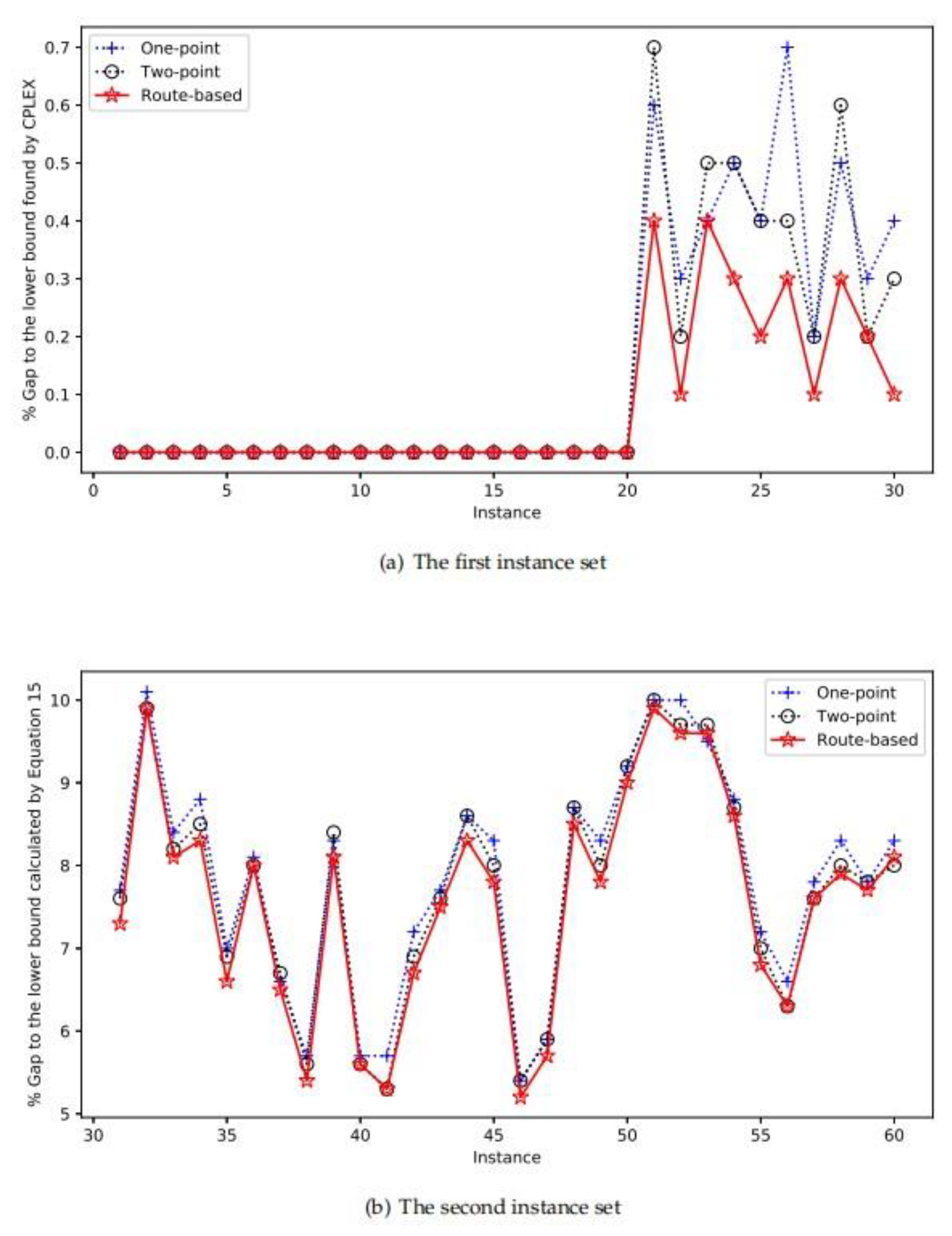
HEA applies the route-based crossover operator presented in Section 3.4 to generate feasible and promising offspring solutions. To study the impact of this crossover operator, we compared HEA with two variants that used only one-point and two-point crossover operators, respectively. Both operators are classic crossover operators used in scheduling and routing problems [26,27], and they can be described as follows. In the one-point crossover operator, the first step is to randomly select one cutting point. The subsequent customer node on one side of the cutting point is copied from a parent solution to the offspring solution. Then, the remaining customers are copied to the offspring solution by keeping the same order unchanged. In the two-point crossover operator, two cutting points are randomly chosen to cut parents. By reference to the two parent solutions S1 and S2, the offspring is generated by firstly copying the subsequent nodes between two cutting points in S1, and then transferring the remaining nodes in the same order from S2. In contrast to the route-based operator, both two reference operators usually generate infeasible solutions, violating the maximum capacity constraint. Hence, we employed the inter-insertion neighborhood operator (N3) to reschedule the position of the conflicting customer node so the infeasible solution could satisfy the maximum capacity constraint.
The experimental condition of this analysis was the same as that of the previous section. The gap to lower bound found by CPLEX and Equation (15) for each test instance is plotted in Figure 7. In terms of the gap indicator, one can observe the better performance of the HEA algorithm when the route-based crossover operator is used, which highlights its importance in HEA.
6. Discussion
The main advantages of the proposed hybrid evolutionary algorithm for MDGVRP can be summarized as follows: First, the variable neighborhood search procedure uses several dedicated neighborhood moves to quickly obtain the local optima for search intensification, which extends the neighborhood operators used in the previous ACO in the literature. Second, the route-based crossover operator and a distance- and quality-based population updating mechanism can effectively enhance the search diversification. Third, the experimental results mentioned above show the proposed HEA method can obtain a better balance in terms of computational efficiency and solution quality in comparison with the ACO algorithm. The limitations of the proposed HEA is that our study only presents the effectiveness of the proposed HEA on the MDGVRP, and the effectiveness on other vehicle routing problems needs to be explored.
7. Conclusions and Future Research
The green vehicle routing problem has emerged as an important and practical problem in green logistics. To help provide effective methods to solve MDGVRP and its related variants, in this study we considered a VRP variant with a realistic multi-depot scenario by harmonizing the environmental and economic costs and determining the assignment of customers to depots. Specifically, we proposed a hybrid evolutionary algorithm (HEA) for MDGVRP. In addition, we demonstrated the effectiveness of the HEA and its key features, which included a variable neighborhood search embedded into several neighborhood operators, a route-based crossover operator utilizing the ideas of iterated greedy strategy, and a distance-and-quality population updating strategy.
Computational results on small-scale and large-scale benchmark instances demonstrate that our proposed HEA performs very favorably compared with the existing heuristic ACO in the literature and the exact solver CPLEX. Particularly, HEA can find better results in terms of solution quality as well as computational speed for both instance sets.
Future work can be extended in the following directions. First, in order to further enhance the search intensification, we can employ the local search breakout to replace the variable neighborhood search. Second, other diversification techniques can be applied for use in these problems such as scatter search or path-relinking. Finally, the effectiveness of the proposed ideas for tackling the MDGVRP suggests that in the future we test the performance for solving other variants of the vehicle routing problems or other similar combinatorial optimization problems in logistics and supply management [28].
Author Contributions
Conceptualization, B.P. and L.W.; methodology, B.P.; software, B.P.; validation, L.W.,; formal analysis, B.P.; investigation, Y.Y.; resources, Y.Y.; data curation, Y.Y.; writing—original draft preparation, B.P.; writing—review and editing, B.P., L.W. and X.C.; visualization, B.P.; supervision, X.C.; project administration, X.C.; funding acquisition, B.P. and X.C. All authors have read and agree to the published version of the manuscript.
Funding
This research was funded by Fundamental Research Funds for the Central Universities of China (Grant Number: JBK2001013 and JBK190504), Key Projects of the National Social Science Fund (Grant Number: 16AJL004), Natural Science Foundation of Zhejiang (Grant Number: LQ19G020002), the 13th Five-Year Plan Teaching Reform Project of Higher Education of Zhejiang (Grant Number: jg20180428), the Project of Education Department of Zhejiang (Grant Number: Y201940902), Basic Scientific Research Project of Wenzhou(Grant Number: R20180002), and Wenzhou Social Sciences Planning Project (Grant Number: 19wsk225).
Conflicts of Interest
The authors declare no conflicts of interest.
References
- Zhou, Y.; Lee, G. A Lagrangian relaxation-based solution method for a green vehicle routing problem to minimize greenhouse gas emissions. Sustainability 2017, 9, 776. [Google Scholar] [CrossRef] [Green Version]
- Ubeda, S.; Arcelus, F.J.; Faulin, J. Green logistics at Eroski: A case study. Int. J. Prod. Econ. 2011, 131, 44–51. [Google Scholar] [CrossRef]
- Guo, J.X.; Tan, X.; Gu, B. The impacts of uncertainties on the carbon mitigation design: Perspective from abatement cost and emission rate. J. Clean. Prod. 2019, 232, 213–223. [Google Scholar] [CrossRef]
- Nocera, S.; Galati, O.I.; Cavallaro, F. On the uncertainty in the economic valuation of carbon emissions from transport. J. Transp. Econ. Policy 2018, 52, 68–94. [Google Scholar]
- Li, J.; Guo, H.; Zhou, Q.; Yang, B. Vehicle Routing and Scheduling Optimization of Ship Steel Distribution Center under Green Shipbuilding Mode. Sustainability 2019, 11, 4248. [Google Scholar] [CrossRef] [Green Version]
- Eun, J.; Song, B.D.; Lee, S.; Lim, D.E. Mathematical Investigation on the Sustainability of UAV Logistics. Sustainability 2019, 11, 5932. [Google Scholar] [CrossRef] [Green Version]
- Lin, C.; Choy, K.L.; Ho, G.T.; Chung, S.H.; Lam, H. Survey of green vehicle routing problem: Past and future trends. Expert Syst. Appl. 2014, 41, 1118–1138. [Google Scholar] [CrossRef]
- Braekers, K.; Ramaekers, K.; Van Nieuwenhuyse, I. The vehicle routing problem: State of the art classification and review. Comput. Ind. Eng. 2016, 99, 300–313. [Google Scholar] [CrossRef]
- Palmer, A. The Development of an Integrated Routing and Carbon Dioxide Emissions Model for Goods Vehicles. Available online: https://dspace.lib.cranfield.ac.uk/handle/1826/2547 (accessed on 7 March 2020).
- Kara, I.; Kara, B.Y.; Yetis, M.K. Energy minimizing vehicle routing problem. In International Conference on Combinatorial Optimization and Applications; Springer: Berlin/Heidelberg, Germany, 2007. [Google Scholar]
- Demir, E.; Bektas, T.; Laporte, G. A comparative analysis of several vehicle emission models for road freight transportation. Transp. Res. Part D Transp. Environ. 2011, 16, 347–357. [Google Scholar] [CrossRef]
- Kopfer, H.W.; Schönberger, J.; Kopfer, H. Reducing greenhouse gas emissions of a heterogeneous vehicle fleet. Flex. Serv. Manuf. J. 2014, 26, 221–248. [Google Scholar] [CrossRef]
- Bektas, T.; Laporte, G. The pollution-routing problem. Transp. Res. Part B Methodol. 2011, 45, 1232–1250. [Google Scholar] [CrossRef]
- Demir, E.; Bektas, T.; Laporte, G. An adaptive large neighborhood search heuristic for the pollution-routing problem. Eur. J. Oper. Res. 2012, 223, 346–359. [Google Scholar] [CrossRef]
- Demir, E.; Bektas¸, T.; Laporte, G. The bi-objective pollution-routing problem. Eur. J. Oper. Res. 2014, 232, 464–478. [Google Scholar] [CrossRef]
- Gajanand, M.; Narendran, T. Green route planning to reduce the environmental impact of distribution. Int. J. Logist. Res. Appl. 2013, 16, 410–432. [Google Scholar] [CrossRef]
- Tiwari, A.; Chang, P.C. A block recombination approach to solve green vehicle routing problem. Int. J. Prod. Econ. 2015, 164, 379–387. [Google Scholar] [CrossRef]
- Suzuki, Y. A dual-objective metaheuristic approach to solve practical pollution routing problem. Int. J. Prod. Econ. 2016, 176, 143–153. [Google Scholar] [CrossRef]
- Jabir, E.; Panicker, V.V.; Sridharan, R. Design and development of a hybrid ant colony-variable neighbourhood search algorithm for a multi-depot green vehicle routing problem. Transp. Res. Part D Transp. Environ. 2017, 57, 422–457. [Google Scholar] [CrossRef]
- Cheng, T.; Peng, B.; Lü, Z. A hybrid evolutionary algorithm to solve the job shop scheduling problem. Ann. Oper. Res. 2016, 242, 223–237. [Google Scholar] [CrossRef]
- Bansal, R.; Srivastava, K.; Srivastava, S. A hybrid evolutionary algorithm for the cutwidth minimization problem. In Proceedings of the 2012 IEEE Congress on Evolutionary Computation, Brisbane, Australia, 10–15 June 2012. [Google Scholar]
- Abdullah, S.; Burke, E.K.; McCollum, B. A hybrid evolutionary approach to the university course timetabling problem. In Proceedings of the 2007 IEEE Congress on Evolutionary Computation, Singapore, 25–28 September 2007. [Google Scholar]
- Wang, Y.; Cai, Z.; Guo, G.; Zhou, Y. Multiobjective optimization and hybrid evolutionary algorithm to solve constrained optimization problems. IEEE Trans. Syst. Man Cybern. Part B 2007, 37, 560–575. [Google Scholar] [CrossRef]
- Karabulut, K.; Tasgetiren, M.F. A variable iterated greedy algorithm for the traveling salesman problem with time windows. Inf. Sci. 2014, 279, 383–395. [Google Scholar] [CrossRef]
- Birattari, M.; Yuan, Z.; Balaprakash, P.; Stützle, T. F-Race and Iterated F-Race: An Overview. In Experimental Methods for the Analysis of Optimization Algorithms; Springer: Berlin/Heidelberg, Germany, 2010; pp. 311–336. [Google Scholar]
- Kellegöz, T.; Toklu, B.; Wilson, J. Comparing efficiencies of genetic crossover operators for one machine total weighted tardiness problem. Appl. Math. Comput. 2008, 199, 590–598. [Google Scholar] [CrossRef]
- Lu, Y.; Hao, J.K.; Wu, Q. Hybrid evolutionary search for the traveling repairman problem with profits. Inf. Sci. 2019, 502, 91–108. [Google Scholar] [CrossRef]
- Zhou, R.; Liao, Y.; Shen, W. Channel selection and fulfillment service contracts in the presence of asymmetric service information. Int. J. Prod. Econ. 2019, 107504. [Google Scholar] [CrossRef]
Figure 1.
Insert customer node 5 between customer nodes 4 and 6 in the same route.

Figure 2.
Exchange the positions of two customer nodes 2 and 5 in the same route.

Figure 3.
Remove customer 7 from the current route and relocate it to a different route.

Figure 4.
Exchange the positions of two different customer nodes 7 and 9 from two different routes.

Figure 5.
Delete two non-adjacent edges (34 and 7D), reverse the intermediate customer nodes (4567) to (7854), and add two new edges (4D and 37) in the same route.
Figure 5.
Delete two non-adjacent edges (34 and 7D), reverse the intermediate customer nodes (4567) to (7854), and add two new edges (4D and 37) in the same route.

Figure 6.
Remove two edges (34) and (7 ) in the first route and two edges (89) and (10 ) in the second route. Then, reverse the intermediate customer nodes (910) to (109) in second route, and add two new edges (310) and (9 ) in the current route. Reverse the intermediate customer nodes (45 6 7) to (76 5 4) in first route, and add two new edges (4 ) and (87) in the current route.

Figure 7.
Comparisons between HEA and its variants that use two crossover operators.


Table 1.
Symbols and the corresponding definitions for the MDGVRP.
| Symbols | Definitions |
|---|---|
| Maximum number of customer nodes | |
| Maximum number of depots | |
| Maximum number of vehicles | |
| 1, if vehicle travels from customer node to customer node , | |
| , , | Customer index and vehicle index, respectively |
| Driving distance from customer node to customer node | |
| Fixed vehicle cost | |
| Variable vehicle cost per unit distance | |
| Volume of fuel consumption per unit vehicle weight per unit distance | |
| CO2 emissions cost per vehicle weight per unit distance | |
| Weight of every transportation product | |
| Average cost per unit weight of CO2 | |
| CO2 emission weight per liter fuel consumption | |
| Average gross weight per vehicle on each route | |
| Requirement of customer node | |
| Ratio of vehicle volume to curb weight | |
| Depot capacity | |
| Vehicle capacity |
Table 2.
Settings of the parameters used in HEA.
| Parameters | Description | Candidate Values | Final Value |
|---|---|---|---|
| The number of individual solutions in the population | {5, 10, 20} | 5 | |
| The threshold of shaking strength in the shaking procedure | 3, 6, 9 | 3 | |
| Interval of threshold ratio values in the shaking procedure | (0,1) | [0.1, 0.2] | |
| Distance factor parameter in the population updating strategy | 0.05,0.1,0.2 | 0.1 |
Table 3.
The performance of the HEA compared with the ACO algorithm and the general solver CPLEX for the first instance set.
Table 3.
The performance of the HEA compared with the ACO algorithm and the general solver CPLEX for the first instance set.
| Instance | m | n | CPLEXLB | CPLEXUB | Gap (%) | ACO | HEA | ||||||
|---|---|---|---|---|---|---|---|---|---|---|---|---|---|
| Gap % | Gap % | ||||||||||||
| 1 | 2 | 9 | 1246.7 | 1246.7 | 0 | 1246.7 | 1246.7 | 1.1 | 0 | 1246.7 | 1246.7 | 0.1 | 0 |
| 2 | 2 | 9 | 1481.6 | 1481.6 | 0 | 1481.6 | 1481.6 | 1.3 | 0 | 1481.6 | 1481.6 | 0.9 | 0 |
| 3 | 2 | 9 | 1434.9 | 1434.9 | 0 | 1434.9 | 1434.9 | 1.5 | 0 | 1434.9 | 1434.9 | 0.2 | 0 |
| 4 | 2 | 9 | 1222.6 | 1222.6 | 0 | 1222.6 | 1222.6 | 0.9 | 0 | 1222.6 | 1222.6 | 0.6 | 0 |
| 5 | 2 | 9 | 1285.7 | 1285.7 | 0 | 1285.7 | 1285.7 | 2.3 | 0 | 1285.7 | 1285.7 | 1.1 | 0 |
| 6 | 2 | 10 | 1688.3 | 1688.3 | 0 | 1688.3 | 1688.3 | 2.8 | 0 | 1688.3 | 1688.3 | 1.1 | 0 |
| 7 | 2 | 10 | 1553.8 | 1553.8 | 0 | 1553.8 | 1553.8 | 1.7 | 0 | 1553.8 | 1553.8 | 0.8 | 0 |
| 8 | 2 | 10 | 1341.8 | 1341.8 | 0 | 1341.8 | 1341.8 | 2.1 | 0 | 1341.8 | 1341.8 | 0.9 | 0 |
| 9 | 2 | 10 | 1464.6 | 1464.6 | 0 | 1464.6 | 1464.6 | 2.8 | 0 | 1464.6 | 1464.6 | 0.5 | 0 |
| 10 | 2 | 10 | 1416.2 | 1416.2 | 0 | 1416.2 | 1416.2 | 2.2 | 0 | 1416.2 | 1416.2 | 0.9 | 0 |
| 11 | 2 | 11 | 1581.8 | 1581.8 | 0 | 1581.8 | 1581.8 | 1.2 | 0 | 1581.8 | 1581.8 | 1.2 | 0 |
| 12 | 2 | 11 | 1769.3 | 1769.3 | 0 | 1769.3 | 1769.3 | 2.9 | 0 | 1769.3 | 1769.3 | 1.9 | 0 |
| 13 | 2 | 11 | 1792.3 | 1792.3 | 0 | 1792.3 | 1792.3 | 1.5 | 0 | 1792.3 | 1792.3 | 2 | 0 |
| 14 | 2 | 11 | 1667.6 | 1667.6 | 0 | 1667.6 | 1667.6 | 1.7 | 0 | 1667.6 | 1667.6 | 0.9 | 0 |
| 15 | 2 | 11 | 1807.9 | 1807.9 | 0 | 1807.9 | 1807.9 | 1.9 | 0 | 1807.9 | 1807.9 | 0.6 | 0 |
| 16 | 2 | 12 | 1807.7 | 1846.2 | 2.1 | 1807.7 | 1892 | 1.8 | 0 | 1807.7 | 1849.4 | 0.3 | 0 |
| 17 | 2 | 12 | 1995 | 2053.7 | 2.9 | 1995 | 2013.1 | 2.1 | 0 | 1995 | 2013.3 | 0.5 | 0 |
| 18 | 2 | 12 | 1839.6 | 1940.2 | 5.5 | 1839.6 | 1861 | 1.6 | 0 | 1839.6 | 1881.6 | 1.9 | 0 |
| 19 | 2 | 12 | 1779 | 1851 | 4.1 | 1779 | 1838.8 | 2.3 | 0 | 1779 | 1780.2 | 1.7 | 0 |
| 20 | 2 | 12 | 1799.7 | 1853.3 | 2.9 | 1799.7 | 1851.1 | 3.5 | 0 | 1799.7 | 1838.7 | 1.6 | 0 |
| 21 | 2 | 13 | 1710.8 | 1765.5 | 3.2 | 1722.8 | 1765.3 | 1.3 | 0.7 | 1717.6 | 1752.2 | 1 | 0.4 |
| 22 | 2 | 13 | 1876.9 | 1928.7 | 2.8 | 1884.4 | 1976 | 3.4 | 0.4 | 1878.8 | 1931.4 | 0.7 | 0.2 |
| 23 | 2 | 13 | 1809.5 | 1916.6 | 5.9 | 1814.9 | 1850.3 | 3.9 | 0.3 | 1816.7 | 1837.9 | 1.4 | 0.5 |
| 24 | 2 | 13 | 1716 | 1802.1 | 5.0 | 1738.3 | 1804.7 | 2 | 1.3 | 1721.1 | 1782.2 | 1.4 | 0.3 |
| 25 | 2 | 13 | 1996.5 | 2097.1 | 5.0 | 2008.5 | 2080.3 | 2.1 | 0.6 | 2000.5 | 2040.5 | 1.1 | 0.2 |
| 26 | 2 | 14 | 1902.2 | 2101.9 | 10.5 | 1921.2 | 1988.7 | 2.3 | 1.2 | 1907.9 | 1943.6 | 1.3 | 0.4 |
| 27 | 2 | 14 | 1718.4 | 1908.6 | 11.1 | 1739 | 1823.3 | 3.9 | 1.2 | 1720.1 | 1764.4 | 2.5 | 0.2 |
| 28 | 2 | 14 | 1759.3 | 2035.5 | 15.8 | 1778.7 | 1794 | 3.8 | 1.1 | 1764.6 | 1807 | 1.1 | 0.4 |
| 29 | 2 | 14 | 1824.3 | 2081 | 14.1 | 1837.1 | 1917.3 | 2.9 | 0.8 | 1827.9 | 1840 | 1.5 | 0.3 |
| 30 | 2 | 14 | 1784 | 2099.4 | 17.7 | 1803.6 | 1833.6 | 2.8 | 1.2 | 1785.8 | 1812.6 | 2.2 | 0.2 |
| #Avg | 1669.1 | 1734.5 | 7.2 | 1674.2 | 1701.5 | 2.3 | 0.8 | 1670.6 | 1687.7 | 1.1 | 0.2 | ||
| #Best | 20 | 21 | 29 | ||||||||||
Table 4.
The performance of HEA compared with the ACO algorithm and the general solver CPLEX for the second instance set.
Table 4.
The performance of HEA compared with the ACO algorithm and the general solver CPLEX for the second instance set.
| Instance | m | n | LB | ACO | HEA | ||||||
|---|---|---|---|---|---|---|---|---|---|---|---|
| Gap % | Gap % | ||||||||||
| 31 | 3 | 20 | 4069.9 | 4688.5 | 4719.7 | 6.3 | 15.2 | 4367 | 4372.3 | 5.7 | 7.3 |
| 32 | 3 | 20 | 4793.2 | 5564.9 | 5638 | 6 | 16.1 | 5267.7 | 5269.7 | 4.9 | 9.9 |
| 33 | 3 | 20 | 3203.6 | 3780.2 | 3832.2 | 5.3 | 18 | 3463.1 | 3490.4 | 2.5 | 8.1 |
| 34 | 3 | 20 | 3972.6 | 4457.3 | 4532.4 | 6.9 | 12.2 | 4302.3 | 4302.7 | 5.8 | 8.3 |
| 35 | 3 | 20 | 3279.2 | 3656.3 | 3686.1 | 7 | 11.5 | 3495.6 | 3507.6 | 2.5 | 6.6 |
| 36 | 3 | 30 | 9361.6 | 11,215.2 | 11,315 | 26.1 | 19.8 | 10,110.5 | 10,139 | 9.6 | 8 |
| 37 | 3 | 30 | 7422.4 | 8172.1 | 8336.9 | 24.2 | 10.1 | 7904.9 | 7924.2 | 7.5 | 6.5 |
| 38 | 3 | 30 | 7160.4 | 8470.8 | 8622.7 | 29.2 | 18.3 | 7547.1 | 7581.8 | 10 | 5.4 |
| 39 | 3 | 30 | 7702.9 | 8935.4 | 8997 | 24.6 | 16 | 8326.8 | 8336.9 | 13.6 | 8.1 |
| 40 | 3 | 30 | 8056.4 | 9506.6 | 9703.6 | 27.6 | 18 | 8507.6 | 8514.9 | 18.7 | 5.6 |
| 41 | 4 | 20 | 3990.3 | 4417.3 | 4499.5 | 6.8 | 10.7 | 4201.8 | 4221.8 | 4.5 | 5.3 |
| 42 | 4 | 20 | 4082.4 | 4535.5 | 4642.9 | 5 | 11.1 | 4355.9 | 4382.8 | 3.1 | 6.7 |
| 43 | 4 | 20 | 6181.6 | 6972.8 | 7063.9 | 8.1 | 12.8 | 6645.2 | 6650.1 | 3.6 | 7.5 |
| 44 | 4 | 20 | 5476.2 | 6127.9 | 6156.8 | 7 | 11.9 | 5930.7 | 5979.6 | 5.1 | 8.3 |
| 45 | 4 | 20 | 6633.6 | 7641.9 | 7754.9 | 5.7 | 15.2 | 7151.3 | 7157.9 | 2 | 7.8 |
| 46 | 4 | 30 | 6239.5 | 7075.6 | 7202.8 | 44.5 | 13.4 | 6564.2 | 6597.9 | 19.2 | 5.2 |
| 47 | 4 | 30 | 6195.4 | 6969.8 | 7067.9 | 40.5 | 12.5 | 6548.5 | 6566.9 | 24.2 | 5.7 |
| 48 | 4 | 30 | 5792.3 | 6881.3 | 7026.6 | 38.9 | 18.8 | 6284.6 | 6346.7 | 23.4 | 8.5 |
| 49 | 4 | 30 | 6537.8 | 7505.4 | 7675.8 | 39.8 | 14.8 | 7047.7 | 7099.2 | 42.9 | 7.8 |
| 50 | 4 | 30 | 6761.8 | 7749 | 7821.1 | 41.6 | 14.6 | 7370.4 | 7376.5 | 36.8 | 9 |
| 51 | 5 | 20 | 5007.4 | 6003.9 | 6147.4 | 12.4 | 19.9 | 5503.1 | 5522.9 | 6.4 | 9.9 |
| 52 | 5 | 20 | 6779 | 7680.6 | 7696.3 | 9.8 | 13.3 | 7429.8 | 7479.1 | 4.2 | 9.6 |
| 53 | 5 | 20 | 3871.4 | 4363.1 | 4442.6 | 8.4 | 12.7 | 4243.1 | 4274.4 | 9.1 | 9.6 |
| 54 | 5 | 20 | 4035.1 | 4600 | 4623.7 | 9.2 | 14 | 4382.1 | 4384 | 3.5 | 8.6 |
| 55 | 5 | 20 | 3057.9 | 3458.5 | 3534.1 | 12.3 | 13.1 | 3265.8 | 3273.1 | 12.5 | 6.8 |
| 56 | 5 | 40 | 6774.6 | 7865.3 | 7931.8 | 32.1 | 16.1 | 7201.4 | 7201.5 | 27.6 | 6.3 |
| 57 | 5 | 40 | 6140 | 6809.3 | 6856.1 | 57 | 10.9 | 6606.6 | 6650.4 | 33.6 | 7.6 |
| 58 | 5 | 40 | 10,628.1 | 11,999.1 | 12,258.4 | 50 | 12.9 | 11,467.7 | 11482 | 38.7 | 7.9 |
| 59 | 5 | 40 | 9201.7 | 10,858.4 | 10,926.1 | 55.7 | 18 | 9910.2 | 9987.8 | 30.9 | 7.7 |
| 60 | 5 | 40 | 8614.4 | 10,268.4 | 10,280.1 | 40.5 | 19.2 | 9312.2 | 9356.1 | 42.7 | 8.1 |
| #Avg | 6034.1 | 6805.9 | 7033.1 | 23 | 14.7 | 6490.5 | 6514.3 | 15.1 | 7.6 | ||
| #Best | 0 | 30 | |||||||||
© 2020 by the authors. Licensee MDPI, Basel, Switzerland. This article is an open access article distributed under the terms and conditions of the Creative Commons Attribution (CC BY) license (http://creativecommons.org/licenses/by/4.0/).
Share and Cite
MDPI and ACS Style
Peng, B.; Wu, L.; Yi, Y.; Chen, X. Solving the Multi-Depot Green Vehicle Routing Problem by a Hybrid Evolutionary Algorithm. Sustainability 2020, 12, 2127. https://0-doi-org.brum.beds.ac.uk/10.3390/su12052127
AMA Style
Peng B, Wu L, Yi Y, Chen X. Solving the Multi-Depot Green Vehicle Routing Problem by a Hybrid Evolutionary Algorithm. Sustainability. 2020; 12(5):2127. https://0-doi-org.brum.beds.ac.uk/10.3390/su12052127
Chicago/Turabian StylePeng, Bo, Lifan Wu, Yuxin Yi, and Xiding Chen. 2020. "Solving the Multi-Depot Green Vehicle Routing Problem by a Hybrid Evolutionary Algorithm" Sustainability 12, no. 5: 2127. https://0-doi-org.brum.beds.ac.uk/10.3390/su12052127
Note that from the first issue of 2016, this journal uses article numbers instead of page numbers. See further details here.