Article

Influences of Nutrient Sources on the Alternation of Nutrient Limitations and Phytoplankton Community in Jiaozhou Bay, Southern Yellow Sea of China

1
Key laboratory of Marine Environment and Ecology, Ocean University of China, Ministry of Education, 238 Songling Road, Qingdao 266100, China
2
Laboratory for Marine Ecology and Environmental Sciences, Qingdao National Laboratory for Marine Science and Technology, Qingdao 266071, China
3
College of Marine Sciences, Hainan University, 58 Renmin Avenue, Haikou 570228, China
4
Center for Marine Environmental Studies, Ehime University, 2-5 Bunkyo-cho, Matsuyama 790-8577, Japan
5
College of Oceanic and Atmospheric Sciences, Ocean University of China, 238 Songling Road, Qingdao 266100, China
*
Author to whom correspondence should be addressed.
Sustainability 2020, 12(6), 2224; https://0-doi-org.brum.beds.ac.uk/10.3390/su12062224
Submission received: 29 January 2020 / Revised: 6 March 2020 / Accepted: 9 March 2020 / Published: 12 March 2020
(This article belongs to the Collection Eutrophication and Sustainable Management of Water)

Abstract

:
A marine ecosystem box model was developed to reproduce the seasonal variations nutrient concentrations and phytoplankton biomasses in Jiaozhou Bay (JZB) of China. Then, by removing each of the external sources of nutrients (river input, aquaculture, wastewater discharge, and atmospheric deposition) in the model calculation, we quantitatively estimated its influences on nutrient structure and the phytoplankton community. Removing the river input of nutrients enhanced silicate (SIL) limitation to diatoms (DIA) and decreased the ratio of DIA to flagellates (FLA); removing the aquaculture input of nutrients decreased FLA biomass because it provided less dissolved inorganic nitrogen (DIN) but more dissolved inorganic phosphate (DIP) as compared to the Redfield ratio; removing the wastewater input of nutrients changed the DIN concentration dramatically, but had a relatively weaker impact on the phytoplankton community than removing the aquaculture input; removing atmospheric deposition had a negligible influence on the model results. Based on these results, we suppose that the change in the external nutrients sources in the past several decades can explain the long-term variations in nutrient structure and phytoplankton community. Actually, the simulations for the 1960s, 1980s, and 2000s in JZB demonstrated the shift of limiting nutrients from DIP to SIL. A reasonable scenario for this is the decrease in riverine SIL and increase in DIP from aquaculture that has reduced DIA biomass, promoted the growth of FLA, and led to the miniaturization of the phytoplankton.

1. Introduction

Coastal areas are regions of transition from terrestrial to ocean environments. The primary production is often high, and the transfer of this productivity through the food web could yield prolific fisheries [1,2]. The growth of phytoplankton in coastal areas can be limited by several factors, including light, temperature, and nutrients [3,4]. Among these, nutrients have attracted the most attention because their input can be human-controlled to reverse eutrophication [5,6,7].
Nutrient elements such as nitrogen (N), phosphorus (P), and silicon (Si) have been reported to be limitation factors for phytoplankton growth and their element ratio may affect community composition [8,9,10,11]. Usually, there are several external sources of nutrients in coastal waters, such as river inputs, exchanges with the marginal seas, and atmospheric deposition. The nutrient loads from these sources are different not only in the amount but also the element ratios, both of which have dramatically changed in past decades under the influences of anthropogenic activities and climate changes [12]. The changes in external sources of nutrients naturally regulate phytoplankton growth, biomass, and species composition, causing fluctuations in the higher trophic species [13], which have been already observed in coastal seas [14,15].
Jiaozhou Bay (JZB) is a semi-enclosed and well-utilized bay in the southwestern Yellow Sea (Figure 1). It has an area of 390 km2 and an average water depth of approximately 7 m [16]. Many observations in JZB have documented the basic characteristics of the seasonal, interannual, and long-term variations in nutrient concentrations and phytoplankton biomasses [17,18,19,20,21]. It is suggested that the important factor controlling the phytoplankton growth in JZB is nutrients [22]. By comparing the nutrient loads and the standing stocks of nutrients in the bay, previous studies indicated that external nutrient sources had decisive effects on the multi-time scale variations of nutrient structures [19,23,24]. However, most of the observations focused on the bay itself, with limited quantitative information about the effects of different nutrient sources on the phytoplankton community composition.
There are several external nutrient sources for JZB. JZB receives fresh water and nutrients from more than ten rivers, among which Dagu River is the largest, accounting for 84% of the total freshwater discharge into the bay [25]. Three of the sewage treatment plants in Qingdao City discharge into JZB directly, i.e., the Haibohe, Licunhe, and Tuandao plants [23]. The fish bait and the excretion of aquaculture species are sources of dissolved inorganic nitrogen (DIN) and dissolved inorganic phosphate (DIP), which can accelerate the eutrophication [26]. Another source of nutrients in JZB is the atmospheric deposition [27]. In addition, the nutrient concentrations are generally higher in JZB than in the Yellow Sea (YS), and the water exchange with the YS removes nutrients from JZB [28]. Many studies calculated the loads of nutrients from these external sources and tried to estimate their contributions to primary production and phytoplankton compositions [23,24]. However, assumption is always necessary in such discussion, because field observation essentially cannot distinguish the nutrients from different sources.
Figure 1. The location and water depths (in meters) of Jiaozhou Bay. The estuary of Dagu River is marked by a star. The observations, including concentrations of three nutrient elements and chlorophyll-a used to validate model results, are shown. Stations of monthly observations from June 2003 to May 2004 carried by [17] are marked by diamonds. Stations of the monthly observations from January 2003 to December 2003 carried by [18] are marked by triangles. Jiaozhou Bay Marine Ecosystem Research Stations from 2004 to 2008 carried by [19] and from January 2011 to December 2011 carried by [29] are marked by dots.
Sustainability 12 02224 g001
Over the last half-century, the external sources of nutrients for JZB have changed under the anthropogenic perturbations [20,21,30]. The diminished river runoff due to the construction of water conservancy projects, the increase in industrial and domestic wastewater discharge, the heavy aquaculture activities, together, have had great impacts on the nutrient structures in JZB over the past few decades [31]. The unbalanced nutrient structure induced serious eutrophication and high frequent occurrences of the harmful algal bloom in JZB [24]. In addition, more DIN and DIP loads but less SIL load into JZB were suggested to decrease the biomass of large-size phytoplankton (DIA) and increase the biomass of small-size phytoplankton (FLA) [19,32]. The miniaturization of the phytoplankton community subsequently hinders energy transport to the higher trophic levels. Some toxic FLA have also caused the collapse of fisheries, along with the loss of several fish species [32,33]. To quantitatively understand the relationship between decadal shifts of nutrient loads of each external source and the nutrient structures and phytoplankton community inside the bay, the correlation analysis used by previous studies is not sufficient, because we need more information to understand the mechanism behind such phenomena.
Numerical modeling is an effective way to reveal the mechanisms linking the external loads of nutrients and the change in nutrient structure and phytoplankton community inside the bay. There have been some related numerical studies [28,34,35]. However, they usually considered one group of phytoplankton (DIA) and failed to reproduce the structure of phytoplankton community. Few studies have considered the role of each external source of nutrients. Therefore, it is still unclear how each external source of nutrients influences the variation in the phytoplankton community of JZB. Considering the small size of the bay and the vertically homogeneous distribution of physical and biogeochemical variables, we choose a box model in this study to quantify the influences of each external source of nutrients on the nutrient concentration and phytoplankton community. The understanding on the temporal changes over the entire bay is also helpful to understand the observations over the bay in the past several decades.
In this study, based on the published estimation of the nutrient loads from various external sources, we establish an ecosystem box model including three kinds of nutrients and two groups of phytoplankton with different cell sizes to quantify the influences of each external source of nutrients on nutrient structure and variation in the phytoplankton community, indicated by the ratio of DIA/FLA. The nutrient limitation conditions for three decades (the 1960s, the 1980s, and the 2000s) are compared to explain the effects of anthropogenic activities on the unbalanced nutrient structure and miniaturization of phytoplankton community.

2. Methods

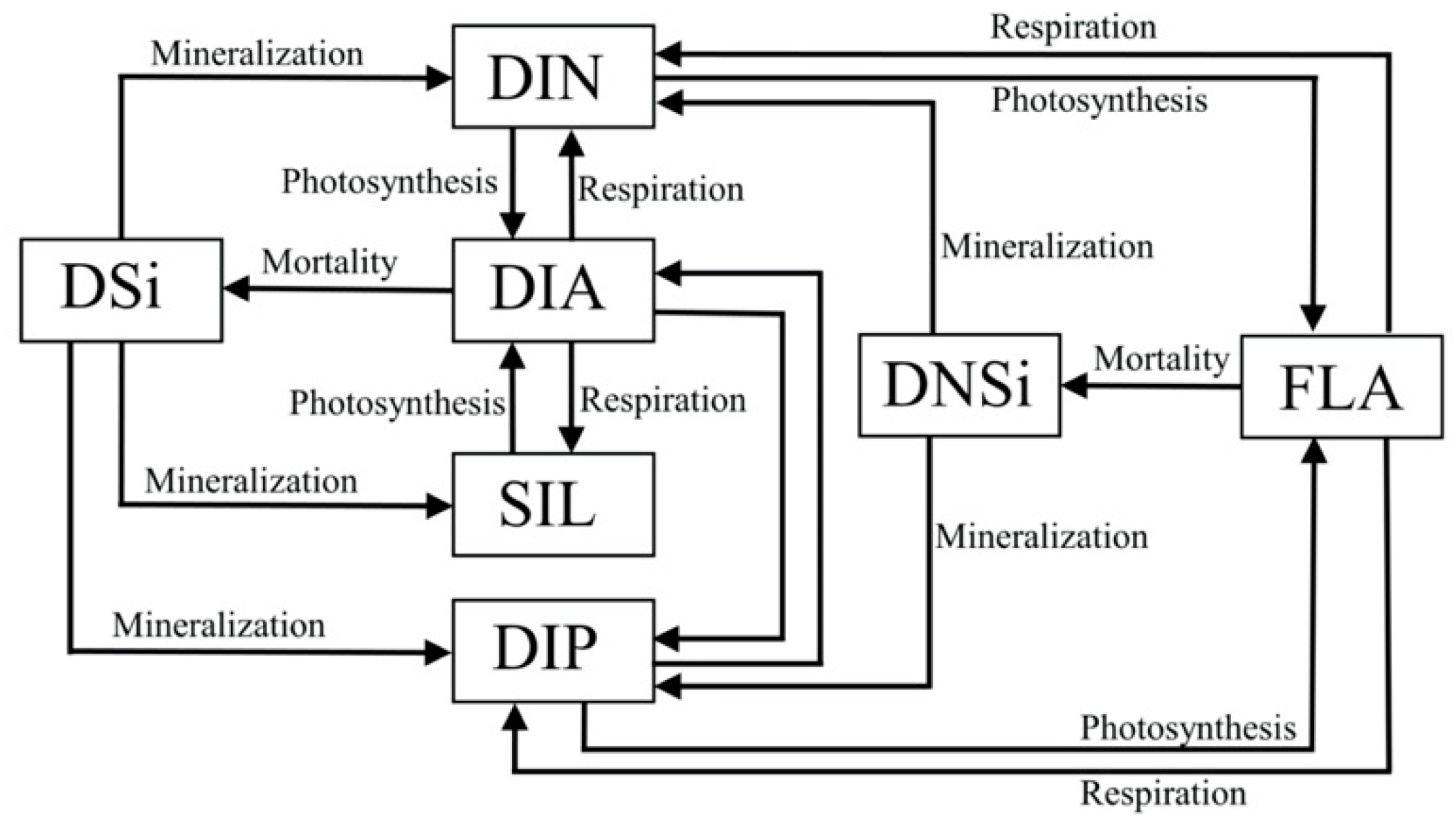
2.1. Model Descriptions

The state variables in this box model included three kinds of nutrients (DIN, DIP, and SIL), two types of phytoplankton (DIA and FLA), and two types of detritus (DSi comprising Si and DNSi not comprising Si). Zooplankton grazing on phytoplankton could be taken into account by increasing the mortality rate of phytoplankton in the numerical model. The biogeochemical processes (Figure 2) among state variables have been studied previously and used in many ecosystem models [36,37]. DIA absorbs DIN, DIP, and SIL for photosynthesis, and releases three types of nutrients through respiration. The mortality of DIA contributes to DSi, which returns to the three types of nutrients through mineralization. The biogeochemical processes of FLA are similar to those of DIA. However, FLA grows depending on DIN and DIP rather than SIL. The mineralization of DNSi releases DIN and DIP. Sources and sinks for different state variables are provided in Appendix A. The parameters used in this model were based on previous studies [28,37] and are given in Table 1. The external sources of nutrients included river input, wastewater discharge, aquaculture, and atmospheric deposition. The exchange amounts of nutrients between the JZB and the YS depend on the differences in concentrations and the average residence time (52 days) (A19). It has been reported that the fluxes from sediments vary by nutrient, site, and redox conditions and directly observed benthic nutrient fluxes are lower than diffusive fluxes calculated from pore waters, indicating that the nutrients released from sediment pore waters are probably utilized in benthic production [27]. Therefore, the nutrients from benthic fluxes were not taken into consideration due to the limited observational data.

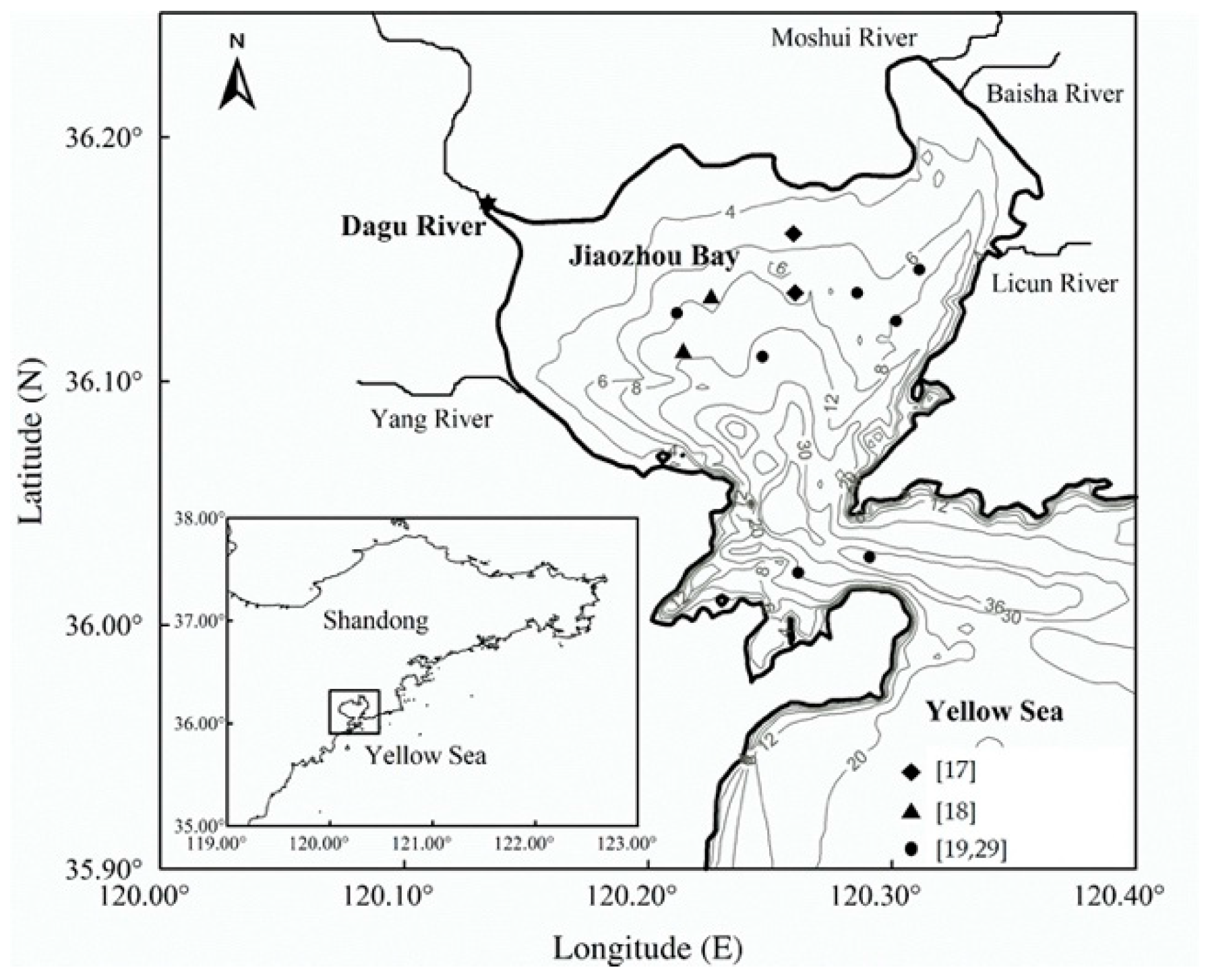
2.2. Model Configuration and Data Sources

2.2.1. CONTROL Run (the 2000s)

The simulation in the 2000s is named CONTROL. The external sources of nutrients were based on observations in the 2000s (Table 2). The amounts of nutrients from rivers depended on both the riverine concentrations of nutrients and the discharge of fresh water (A18). In this model, only Dagu River was taken into consideration, and the other small rivers were ignored. The river discharge (in L   s 1 ) of the Dagu River in the 2000s was derived from the model results of the Soil and Water Assessment Tool (SWAT) [38]. The river discharge reached its peak in summer (July to September), up to 9.0 × 10⁴ L   s 1 , and remained low in other seasons, especially in winter (December to February), with an annual total discharge of 3.0 × 10¹¹ L. The riverine concentrations of DIN, DIP, and SIL were based on observations in 2002 [23]. The annual amount of nutrients from wastewater was obtained from investigations in 2002 [23]. The annual aquaculture input was estimated from aquaculture conditions in 2008 [39]. Atmospheric depositions of nutrients, including wet and dry deposition, were based on rainwater and aerosol samples collected at the coastal site of JZB from April 2004 to March 2005 [27]. Nutrients from these three external sources (wastewater, aquaculture, and atmosphere) were assumed to have little seasonal variations, and the annual amounts were averaged to each time step for model calculation. The concentrations of nutrients in the YS were set to 6.0, 0.3, and 4.0 μ mol   L 1 for DIN, DIP, and SIL, respectively, according to observations [18,40].
The physical forcing includes the annual cycles of sea surface light intensity (I0, in W m−2) and seawater temperature (Temp, in °C), expressed by the following cosine functions of time (t in Julian Day) [42]:
I 0 = 240 140 × cos [ 2 π × t + 10 365 ] ,
Temp = 13.5 11.0 × cos [ 2 π × t 40 365 ] .
The average light intensity (I) in JZB is expressed as I = 0.4 × I0, considering the light attenuation due to pure water and suspended particulate materials in the water column, which is derived in Appendix A.
The initial conditions of state variables were based on observed data from the winters of the 2000s [17,18]. The initial concentrations of DIN, DIP, and SIL were set to 13.0, 0.8, and 6.0 μ mol   L 1 , respectively. The initial biomasses of DIA and FLA were 0.72 and 0.08 μ g   L 3 , respectively, in the form of chlorophyll-a (Chl-a) concentrations. After running the model for three years, the outputs were close to the climatological state of the model. The outputs of the fifth year were used in the following analysis.
The data used to validate the model results were the averaged values of several observations in the 2000s (Figure 1) [17,18,19,29].

2.2.2. NORI, NOWA, NOAQ, and NOAT Runs

In order to examine the different effects of the external nutrient sources, four numerical experiments were carried out and named NORI, NOWA, NOAQ, and NOAT, in which nutrients were removed from river input, wastewater discharge, aquaculture activities, and atmospheric deposition, respectively. Except for removing one external source of nutrients, the other conditions used in these experiments were the same as CONTROL.

2.2.3. The 1960s and the 1980s Runs

As shown in Table 2, the runoff of the Dagu River decreased from 7.5 × 10¹¹ L   y 1 in the 1960s to 5.0 × 10¹¹ L   y 1 in the 1980s [38,43]. The riverine concentration of SIL in the 1960s and the 1980s was supposed to be proportional to the sediment loads of Dagu River, which were approximately four and three times the amount of that in the 2000s, respectively [41,43]. The SIL concentration in the river decreased from 600 μ mol   L 1 in the 1960s to 420 μ mol   L 1 in the 1980s (Table 2). The DIN (DIP) concentration in the river increased from 60 (3.0) μ mol   L 1 in the 1960s to 260 (5.3) μ mol   L 1 in the 1980s [23,41]. It was reported by the Qingdao Statistical Yearbook in 2005 that the amount of industrial and domestic wastewater increased dramatically in the past 20 years. The amount of wastewater in the 2000s was nearly twice that in the 1980s [19]. The nutrient loads in the 1980s were estimated to be 40% of the values in the 2000s, proportional to the amount of wastewater (Table 2). In the 1960s, industry activities were rarely thriving; therefore, the nutrients from wastewater discharge can be neglected. The amounts of DIN and DIP from aquaculture activities in the 1980s were estimated to be 1.8 × 10⁶ mol   y 1 and 0.12 × 10⁶ mol   y 1 due to the variation in aquaculture areas [24,44], while nutrients from aquaculture were ignored in the 1960s. Nutrients from atmospheric deposition in the 1960s and 1980s were regarded to be the same as those in the 2000s due to the data limitation.
Although the human-induced changes in the coastline position-configuration and nearshore bathymetry have resulted in substantial changes to the residual current patterns, especially in northeastern JZB, the average residence time did not change apparently from 1966 to 2008 [45]. The same residence time of 52 days was used to calculate the exchange with YS, but the nutrient concentrations of YS changed a lot for different times (Table 2). The annual cycles of sea surface light intensity and seawater temperature were treated the same as the CONTROL Run.

3. Results

3.1. Parameter Sensitivity Analysis

Model sensitivity experiments were conducted to examine how the predicted variables vary with the changes of the model parameters within a given range (Table 3). The predicted state variables in these sensitivity experiments were the annual mean biomasses of DIA and FLA. Taking the parameters listed in Table 1 as the control run, the value of any selected parameter was increased and decreased by 50%. The model was run for three years in each sensitivity experiment, and the results of the third year were used. The sensitivity of a predicted state variable to the selected parameter was quantified as a factor s = | Δ A / A | | Δ B / B | , where A is the mean biomass of DIA or FLA and B is the value of one model parameter. ∆A is the variation of A when the parameter varies by ∆B.
The annual mean biomasses of DIA and FLA are sensitive to their own maximum growth rate and mortality rate (s > 0.5). The sensitivity factors about the basic respiration were 0.34 and 0.22 for DIA and FLA, respectively. The annual mean biomass of DIA was more sensitive to the half saturation constant of SIL (s = 0.31−0.39) than those of DIN (s = 0) and DIP (s = 0), while that of FLA was more sensitive to its half-saturation constant of DIP (s = 0.17−0.20) than that of DIN (s = 0). The sensitivity of the half saturation constant of DIN was low, indicating that the growth of DIA and FLA is not limited by DIN. The sensitivity analysis also quantified the competition between the two types of phytoplankton. The annual mean biomass of FLA had a sensitivity to some parameters related to the growth of DIA, such as the maximum growth rate of DIA (s = 0.12−0.13), the optimum light intensity for DIA (s = 0.11−0.12), but not vice versa. It is suggested that DIA is more competitive than FLA. On the other hand, the limiting nutrients for both DIA and FLA did not change when changing the model parameters with a large range (i.e., 50%). Evidently, the model-based conclusions on limiting nutrient and the phytoplankton community are robust.

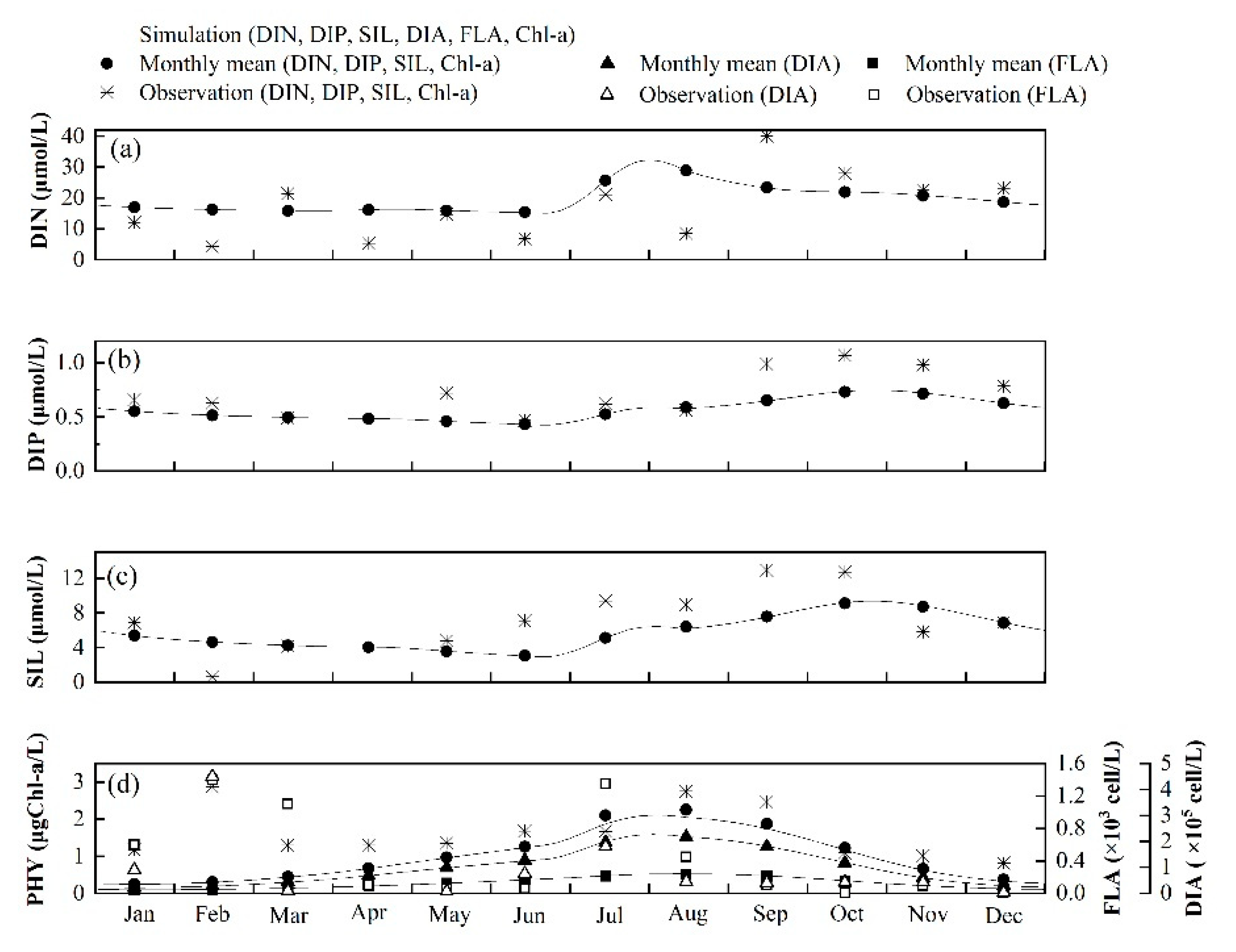
3.2. Seasonal Variations of Nutrient Concentrations and Phytoplankton Biomasses

The simulated concentrations of the three types of nutrients in JZB exhibited apparent seasonal variations (Figure 3). All three nutrient elements accumulated in winter, when the growth of phytoplankton is limited by low water temperature and weak solar radiation. Then, the concentrations of DIN, DIP, and SIL decreased to about half of their peak values in spring along with the vigorous primary production. In summer, the concentrations increased gradually due to the large river input, and the concentrations of DIN and SIL increased more significantly than DIP. In autumn, the concentrations of DIP and SIL continuously increased in response to the reduction of phytoplankton photosynthesis. However, the concentrations of DIN decreased slightly due to the low river input.
The biomasses of both DIA and FLA experienced an apparent bloom in summer and had their lowest value in winter. The biomasses of DIA and FLA reached the peak values of 1.52 μ g   L 1 and 0.52 μ g   L 1 in August (Figure 3d), respectively, consistent with the maximum river runoff in summer. The biomass of DIA was higher than that of FLA throughout the year, especially in summer. The annual mean ratio of DIA to FLA was 2.3, with the maximum value of 2.9 in August and the minimum value of 1.6 in January. Therefore, DIA is the dominant phytoplankton species in JZB, which is consistent with the observations by [46], accounting for approximately 75% of the total phytoplankton in August.
It has been reported that there is a significant correlation between Chl-a and phytoplankton density when the dominant phytoplankton species are stable [47]. Since the biomasses of DIA and FLA represented by Chl-a concentrations could not be observed, the observed monthly density of DIA and FLA were used to validate the modeled seasonal variations of Chl-a concentrations. DIA density was obviously higher than that of FLA all throughout the year, and they both experienced similar seasonal variations with the peak in summer, which could also be captured by the modeled Chl-a concentrations of DIA and FLA [29]. Observations in JZB showed two phytoplankton blooms occurring in February and August [48,49]. Appearance of some cold-water species is suggested to be responsible for the February bloom [18]. Because the two types of phytoplankton in our model did not represent the cold-water species, we could not reproduce the bloom in February. Since the cold-water species of phytoplankton did not appear every February [19], the model was able to simulate the main seasonal variations of nutrient concentrations and phytoplankton biomasses in JZB.

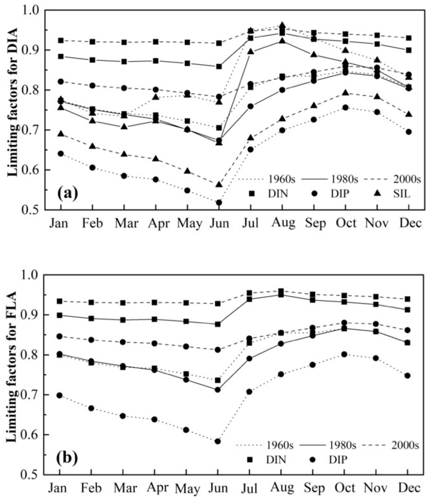
3.3. Seasonal Variations of Nutrient Limitations

The nutrient limitations on the growth of phytoplankton are given by the minimum value of the three factors ( DIN lim = DIN / ( DIN + K DIN ) ,   DIP lim = DIP / ( DIP + K DIP ) ,   SIL lim = SIL / ( SIL + K SIL ) ), where K DIN ,   K DIP ,   K SIL are half-saturation constants (in Appendix A). The limiting nutrient in JZB was determined through comparing the value of three factors. The simulated annual mean concentrations of the DIN, DIP, and SIL were 19.8, 0.56, and 5.73 μ mol   L 1 ), respectively. The ratio of DIN/DIP was 38/1, much larger than the Redfield ratio. Both the high concentration of DIN and the ratio of DIN/DIP suggest that DIN was in surplus compared with DIP. As shown in Figure 4, the values of DIN lim for DIA and FLA were above 0.9 during the whole year, suggesting that DIN never served as the limiting nutrient for the growth of phytoplankton. The limiting nutrient for DIA was SIL all year around (Figure 4). The SILlim decreased from January to June, and the limitation effect was strongest in June, when its value was 0.56. Then, the limitation effect gradually weakened due to the riverine SIL input in summer. The growth of FLA was limited by DIP (Figure 4) all year round. The mean DIPlim for it was about 0.82, which was always higher than the SILlim for DIA. Given that DIA is the dominant species in JZB, SILlim appears favorable for controlling the ecological equilibrium of JZB.

3.4. Annual Budgets of Nutrients

Figure 5 shows the annual budgets of DIN, DIP, and SIL. The four external sources of nutrients (river, wastewater, aquaculture, and atmosphere) were treated as forcing conditions in the model. Their amounts are listed in Table 2. The budgets of biogeochemical processes represent the renewal and cycle rate of nutrients in JZB. Phytoplankton plays an important role in the renewal of nutrients. The net production of phytoplankton (photosynthesis minus respiration) is the main sink, with 316.89 × 10⁶ mol   y 1 of DIN, 19.81 × 10⁶ mol   y 1 of DIP and 382.37 × 10⁶   mol   y 1 of SIL. The maximum net production of DIA and FLA occurred in summer, consistent with their high biomasses. The mineralization of detritus released 317.19 × 10⁶ mol   y 1 of DIN, 19.83 × 10⁶ mol   y 1 of DIP, and 382.76 × 10⁶ mol   y 1 of SIL, which are approximately 70% of the amount of photosynthesis absorption. According to the model results, the annual mean concentrations of the three nutrients in JZB are higher than those in YS. Annually, 432.09 × 10⁶ mol of DIN, 8.36 × 10⁶ mol of DIP, and 54.70 × 10⁶ mol of SIL are transported out from JZB to YS through water exchange. The nutrient budgets are in balance in the whole year, which indicates that the model followed the mass conservation.

3.5. Estimation of the Contributions of Nutrient External Sources on Nutrient Limitations and Phytoplankton Community

The responses of the nutrients and phytoplankton structures in JZB to each external nutrient source were examined by comparing the results of NORI, NOWA, NOAQ, and NOAT with those of CONTROL (Figure 6 and Figure 7). The nutrients flux of atmospheric deposition was the smallest among the four external sources. The DIA and FLA biomasses decreased slightly by 0.2% and 0.5% in NOAT, respectively. Removing atmospheric deposition had a negligible influence on the model results of both phytoplankton biomasses and nutrient concentrations. The results of the other three experiments are discussed in detail bellow.

3.5.1. The Effects of River Input

The Dagu River inputs 45.79 × 10⁶ mol SIL into JZB per year, contributing up to 80% of the annual amount from the four external sources. Meanwhile, it is a large source of DIN (122.10 × 10⁶ mol y−1), just less than that from wastewater discharge. The amount of DIP from river input is 2.14 × 10⁶ mol y−1, which is similar as that from wastewater but much less than that from aquaculture.
Comparing the results of NORI with those of CONTROL, the annual mean concentrations of DIN, DIP, and SIL decreased by 19%, 11%, and 25%, respectively. The decreases are apparent in all these three nutrient elements (Figure 6). Moreover, the nutrient supply from the river exhibited an obvious seasonal variation due to the significantly different runoff during the wet and dry seasons. As a result, nutrient concentrations hardly changed in the dry seasons and changed a lot in the wet seasons. In summer, the peak of DIN disappeared in NORI, and the concentration of DIN increased from July, and then began to decline after reaching the peak in November (Figure 6a). The concentrations of DIP and SIL decreased continuously in summer in NORI rather than increase in CONTROL (Figure 6b,c). After reaching the trough in July, the DIP and SIL concentrations in NORI increased from August, and then began to decrease after reaching the peak in November. The peak time was one month later than other numerical experiments. The maximum decrease of SIL and DIP also occurred in summer, when the values were only half those in CONTROL.
The values of SIL and DIP limiting factors in NORI decreased evidently in summer, enhancing the SIL limitation for DIA and DIP limitation for FLA (Figure 7). The SIL limiting factor in spring and winter changed relatively slightly. SIL still acted as the limiting nutrient for the growth of DIA all year round, but SIL limitation was strengthened in NORI (Figure 7).
The annual biomass of DIA decreased by 17%, while the decreasing percentage of FLA was only 3%. The biomasses of DIA and FLA changed the most in summer, which were reduced by 30% and 6%, respectively. The annual mean ratio of DIA to FLA decreased from 2.3 to 2.0, indicating that the river input of nutrients has stronger influences on DIA than on FLA. The enhanced SIL limitation leads to a phytoplankton structure favored to FLA.

3.5.2. The Effects of Aquaculture Activities

Aquaculture provides 54 × 106 mol y−1 DIN to JZB, which is similar to the amount from atmospheric deposition, but only a quarter of that from wastewater discharge. However, it is the main source of DIP, with an annual amount nearly twice that from wastewater or river. The ratio of DIN to DIP from aquaculture is 14, indicating that aquaculture is the only source with a lower ratio of DIN/DIP than the Redfield ratio.
DIN concentration in NOAQ exhibited similar seasonal variations as that in CONTROL, but the value was about 2.0 μ mol   L 1 less than that in CONTROL (Figure 6a). Among the results of CONTROL and four experiments, the DIP concentration in NOAQ almost maintained the lowest throughout the year (Figure 6b), only slightly larger than that in NORI in summer. No SIL comes from aquaculture, so the SIL concentration did not change in NOAQ.
The DIP limiting factor for FLA decreased by 0.05 compared with that in CONTROL (Figure 7). The FLA biomass decreased by 5% annually and changed the most in June, which was decreased by 8%, while the DIA biomass had nearly no change all year round without this source. The ratio of DIA to FLA increased from 2.3 in CONTROL to 2.4 in NOAQ. Therefore, FLA is more sensitive to this source than DIA, and aquaculture activities have effects on the miniaturization of phytoplankton size.

3.5.3. The Effects of Wastewater Discharge

Wastewater is the largest source of DIN, with an annual amount of 200 × 106 mol y−1, which is nearly twice that from rivers. However, it only contributes half of the amount of DIP from aquaculture and one sixth of the amount of SIL from rivers. The ratio of DIN/DIP/SIL is approximately 100/1/4 in wastewater (Figure 5), which suggests that wastewater brings more DIN into JZB compared with DIP and SIL.
The seasonal variations of nutrient concentrations, nutrient limiting factors, and phytoplankton biomasses in NOWA were similar to those in CONTROL (Figure 6). However, the values were different, especially for DIN concentration. DIN concentration in NOWA remained the lowest among the four experiments nearly all year round, and only larger than that in NORI in summer (Figure 6a). DIP concentration in NOWA was also lower than that in CONTROL all through the year, however there was even no considerable change in SIL concentration. Wastewater discharge brings more excessive DIN into JZB, therefore, the limiting factors of SIL for DIA and DIP for FLA in NOWA became smaller than those in CONTROL, indicating a strengthened SIL limitation for DIA and DIP limitation for FLA.
FLA biomass decreased by 3%, while DIA biomass decreased by 2% annually in NOWA. Seasonally, the DIA and FLA biomasses decreased more in winter and spring than in summer and autumn, because the river input relieved the unbalance of nutrient structures caused by the wastewater discharge in summer. In general, the ratio of DIA to FLA increased slightly annually.

3.5.4. The Effects of External Sources on the Cycling Rate of Nutrients in JZB and the Exchange with the YS

Besides the changes in the nutrient concentrations and phytoplankton biomasses in JZB when removing each external source of nutrients, the cycling rates of nutrients among different state variables exhibited even more apparent variations, which could not be revealed directly by in-site observations. Comparing the annual budgets of SIL in NORI and CONTROL (Table 4), the annual photosynthesis of DIA was 366.15 × 10⁶ mol SIL when removing river input, which is about 33% less than that in CONTROL. Meanwhile, the respiration of DIA and the mineralization of DSi decreased by about 37%. The decrease in each biochemical process of SIL cycle is even more apparent than that in the standing stocks of SIL in JZB when removing river input. Similar situations occurred in the DIP cycle when removing nutrients from aquaculture. The annual amount of DIP related process (the photosynthesis and respiration of FLA, the mineralization of DNSi) decreased up to 10% when removing aquaculture, while the decrease in annual FLA biomass was 5%. These variations in NOWA are not as much as those in NORI and NOAQ. That is because wastewater discharges mainly DIN to JZB, which is not the limiting nutrient. Therefore, it can be concluded that removing external sources of limiting nutrients obviously slows down the cycling rate of nutrients in JZB.
In addition, there were obvious decreases in the exchanging amounts of nutrients with the YS in these four numerical experiments. When removing river input, the transporting amount of SIL from JZB to the YS decreased from 54.70 × 10⁶ mol y−1 to 8.92 × 10⁶ mol y−1. Wastewater discharge has less influence on the phytoplankton biomasses than river input and aquaculture activities. However, the exchanging amount of DIN in NOWA decreased to only half of that in CONTROL. So, besides the effects on JZB itself, the external sources of nutrients have more remote influences on the adjacent seas through water exchange controlled by complicated hydrodynamic processes.

3.6. Long-Term Variations of the Nutrient Limitation and Phytoplankton Community

As shown in Section 3.5, the external sources of nutrients have various influences on the nutrient structure and phytoplankton community in the JZB. Since the nutrient loads from the external sources have dramatically changed by human activities in the past several decades, it may result in changes in nutrient limitation and then the phytoplankton community in JZB. Considering different amounts of nutrients from the four external sources in different decades (Table 2), the model reproduced the nutrient structure and phytoplankton community in the 1960s and the 1980s.
The annual cycles of nutrient concentrations and phytoplankton biomasses in these two decades showed similar seasonal patterns to the results in the 2000s. The simulated concentrations of DIN and DIP in the 1960s were in good agreement with the observations (Table 5). The concentration of SIL in the 1960s could not be evaluated due to there being too few observations. The simulated concentrations of DIN, DIP, and SIL in the 1980s almost fell into the ranges of observations in this decade (Table 5). The concentrations of DIN and DIP in the 2000s were about six times and triple those in the 1960s, respectively. However, the SIL concentration in the 2000s was only half of that in the 1980s and one quarter of that in the 1960s.
The increase in DIN was mainly caused by the river input and wastewater discharge. The river input was determined by both the runoff and the riverine concentrations. Although the annual river runoff decreased from 7.5 × 10¹¹ L in the 1960s to 3.0 × 10¹¹ L in the 2000s, the annual amount of DIN from the river still increased from 45 × 106 mol in the 1960s to 120 × 106 mol in the 2000s due to the dramatic increase of the riverine DIN concentration. The continuously prosperous industry brought about more and more wastewater, which made wastewater become the biggest source of DIN until the 2000s (Table 2). Consequently, the annual DIN input from the four external sources increased from 101 × 106 mol in the 1960s to 268 × 106 mol in the 1980s, and then reached 430 × 106 mol in the 2000s. The expansion of aquaculture activities was mainly responsible for the rising input of DIP to JZB. The total DIP input increased from 2.67 × 10⁶ mol in the 1960s to 3.99 × 10⁶ mol in the 1980s, then to 8.32 × 10⁶ mol in the 2000s. Overall, the DIN concentration in JZB experienced a faster increase than that of DIP. On the contrary, the concentration of SIL showed an apparently decreasing trend from the 1960s to the 2000s (Table 5), which was definitely caused by the decreases in both the river runoff and the riverine SIL concentration.
The long-term variations in nutrient concentrations changed the nutrient limitation situations and the phytoplankton compositions in JZB. In the 1960s, the limiting nutrient for both DIA and FLA was DIP (Figure 4). The DIP limiting factor for DIA was smaller than that for FLA due to the larger DIP half-saturation constant for DIA, indicating the stronger limitation for DIA. However, the dominant species was still DIA, due to its larger maximum growth rate. The annual mean ratio of DIA to FLA was approximately 2.7. The nutrient limitation in the 1980s changed dramatically compared with the situation in the 1960s. DIP was still the limiting nutrient for FLA. However, DIP and SIL alternatively limited the growth of DIA in the 1980s (Figure 4a). From January to June, the limiting factor of SIL ( SIL lim ) was smaller than that of DIP ( D I P l i m ), indicating the concentration of SIL controlling the growth of DIA. From July to November (the flood season), the limiting nutrient shifted from SIL to DIP. Although the concentration of SIL decreased from the 1960s to the 1980s, the increasing wastewater discharge and aquaculture activities brought a large amount of DIP and relieved the DIP limitation, making nutrient limitation in the 1980s weaker than the situation in the 1960s. As a result, the annual mean biomass of DIA increased from the 1960s (0.64 μ g   L 1 ) to the 1980s (0.80 μ g   L 1 ). The annual ratio of DIA to FLA in the 1980s was approximately 2.9, which was larger than that in the 1960s. The ecosystem in JZB changed from DIP limitation to SIL limitation under the influence of reduced SIL input, and relatively increased DIP input from the 1980s to the 2000s. The enhanced SIL limitation from the 1980s to the 2000s (Figure 4a) led to a more apparent increase in FLA biomass and a comparatively insignificant increase of DIA biomass. The annual ratio of DIA to FLA greatly reduced from 2.9 to 2.3, which resulted in the miniaturization of the phytoplankton community.

4. Implications and Limitations

The nutrient limitation may be caused by low concentrations or alternations due to changing ratios. The more obvious changes in phytoplankton are not in the biomass, but in the community composition in JZB. This shift in phytoplankton species was mainly caused by the change in nutrient ratios. From the 1980s to the 2000s, the DIN/DIP/SIL changed from 31/1/26 to 35/1/10, according to the model results. The increases in DIN and DIP concentrations (especially DIN) and the decrease in SIL concentration resulted in a more unbalanced nutrient structure [50]. DIP limitation for DIA growth has almost been eliminated. Meanwhile, strengthened SIL limitation has led to the decrease of DIA, and the smaller species have taken over the niche vacated by the larger species [20].
River input is the main source of SIL, and therefore becomes the only source to support a diatom dominant phytoplankton community in JZB. Damming usually decreases SIL load, which makes SIL a potential limiting nutrient in coastal waters [51,52], such as Guadiana estuaries in Mediterranean [53], Sweden, Finland [54], and the Baltic Sea [14]. The sharp decrease of SIL flux caused higher frequency of occurrence of harmful algal bloom [55,56]. In addition, low SIL concentration limited the silicification ability of DIA, and then reduced their absorption of Cd in the seawater, which finally resulted in heavy metal pollution [57] and toxin enrichment through the aquatic food chain [58]. In the North Sea, more reduction in riverine P loads than N loads caused large offshore gradient of DIN/DIP ratio in spring, from 375:1 nearshore toward 1:1 in the central North Sea and the phytoplankton growth was limited by P and Si nearshore, co-limited by N and P in a transitional region, and limited by N in the outer-shore waters [59].
Nutrients from aquaculture, with a lower DIN/DIP ratio compared with those from other nutrient sources, led to the more obvious growth of FLA than that of DIA in JZB. It was reported that the phytoplankton community experienced a shift from DIA-dominated to FLA-dominated based on observations in an offshore shellfish-cultured area located in the northern Yellow Sea of China [60]. There was also a worldwide phenomenon that excessive discharge of DIP increased the risks of eutrophication and threatened the environmental regulations in the aquaculture waters [61]. So, the utilization efficiency of nutrients was regarded to be an important indicator, whether the aquaculture activities were sustainable or not [60]. In addition, it has been reported that aluminum pillared bentonite can decrease the P loads from aquaculture, and it can be used for the treatment of aquaculture discharge water before releasing into the coastal seas [62].
The effects of wastewater vary due to its various components in different countries. A previous study [63] reported that the low N/P ratio of wastewater inputs resulted in a DIN-limited and DIP-saturated system in the estuaries of Chesapeake Bay, which is totally different from the situation in JZB. Reduced loads of nutrients from the Luggage Point sewage treatment plants into the Moreton Bay resulted in a decrease in DIN concentration and phytoplankton biomass [64]. In the Scheldt estuary of the Netherlands, upgrading the wastewater treatment plant dramatically reduced DIN and DIP delivery to the coastal seas. In the absence of decreases in SIL export, the reduction of DIN and DIP fluxes and the improvement of the DIN/DIP ratio compared to SIL favored the growth of DIA [65]. After decreases in N and P inputs through a wastewater-improvement project, the trophic status shifted from hyper-eutrophic to eutrophic-mesotrophic in Boston Harbor. As a result, the N limitation relative to P limitation increased and the primary production and phytoplankton biomass decreased [66]. Nitrogen reduction reduced the winter spring diatom bloom and winter Chl-a levels were lower significantly after nutrient reduction in Narragansett Bay [67].
The model results showed that the atmospheric deposition had little influence on the variations in phytoplankton biomass and composition in JZB. The atmospheric deposition provided a similar amount of DIN to JZB compared with the aquaculture. However, it brought less DIP and SIL, which acted as the limitation nutrients in JZB in the 2000s. It was widely reported that atmospheric deposition was an important source of nutrients and promoted primary production in open oceans [68,69]. The atmospheric deposition of nitrogen contributed about 10% of the primary production in the western Pacific Ocean [70]. Even in regional seas, the atmospheric deposition is also an important source of nutrients. Taking YS for example, the estimated annual amount of nitrogen from atmospheric deposition was about five times that from the rivers. However, their contributions to the annual primary production of the whole Yellow Sea were not very high, because there was already surplus DIN in the seawaters. Only in certain areas and certain periods can their contributions not be neglected. The nitrogen from atmospheric deposition promoted the spring phytoplankton bloom in the central part of the Yellow Sea when DIN was used up by the fast growth of phytoplankton [71]. During heavy-polluting weathers, such as dust or haze events, the amount of nitrogen from atmospheric deposition increased to twice as much as that in normal days [72], which aggravated the DIP and SIL limitation situation and then affected the composition of the phytoplankton community [73].
It was also indicated by the nutrient budgets that the external sources of nutrients have subsequent effects on the adjacent seas besides the bay itself. When considering the effects of climate change, the remote influences of the oceans on the marginal seas always gain more attraction. However, it cannot be neglected that anthropogenic activities can also affect the remote oceans through coastal waters and marginal seas. For example, the material exchange between the East China Sea shelf (marginal sea) and Kuroshio affects not only the ecosystem of the East China Sea but also that of the Northwestern Pacific Ocean [37,74,75].
It should be noted that the influence discussed above primarily focuses on the entire JZB. The box ecosystem model was effective when focusing on the temporal variation of nutrient composition and succession of the phytoplankton community of the entire JZB under the influence of anthropogenic activities. However, it could not differentiate the spatial variations in JZB due to inhomogeneity of the nutrient sources, e.g., the aquaculture activities and wastewater have more significant impacts on shore areas. In addition, the nutrients from benthic fluxes were not taken into consideration due to the limited observational data. This is, however, probably important to the shore area because of presence of large tidal flat in JZB. Therefore, a fully three-dimensional model with a moving boundary at shore area is probably necessary in the future to further understand the spatial variation in the bay.

5. Conclusions

The simulated annual cycles of nutrient concentrations and phytoplankton biomasses in the 2000s suggest that the growth of DIA is limited by SIL, while that of FLA is limited by DIP. Changes in the external nutrient sources lead to long-term variations (the 1960s, the 1980s, and the 2000s) in nutrient limitation and the phytoplankton community. Removing the nutrients from the river input enhances SIL limitation for DIA and decreases the ratio of DIA to FLA from 2.3 to 2.0. Aquaculture activities are the main source of DIP; therefore, the FLA biomass decreases when removing this external source. The wastewater has a relatively weaker impact on the change of phytoplankton communities than aquaculture, and the influence of atmospheric deposition is likely negligible.

Author Contributions

Conceptualization, J.S., H.G. and X.G.; methodology, Q.L. and X.M.; validation, Q.L. and J.Z.; formal analysis, Q.L.; writing—original draft preparation, J.S.; writing—review and editing, Q.L., J.S. and X.G. All authors have read and agreed to the published version of the manuscript.

Funding

This research was funded by Youth Talent Support Program of the Laboratory for Marine Ecology and Environmental Science, Pilot National Laboratory for Marine Science and Technology (Qingdao), grant number LMEES-YTSP-2018-02-03; the National Natural Science Foundation of China-Shandong Joint Fund for Marine Ecology and Environmental Sciences, grant number U1606404.

Acknowledgments

We would like to thank Pu Xiang who provided the discharge of Dagu River and Liu Sumei who provided the data of nutrient sources in the 2000s.

Conflicts of Interest

The authors declare no conflict of interest. The funders had no role in the design of the study; in the collection, analyses, or interpretation of data; in the writing of the manuscript, or in the decision to publish the results.

Appendix A

The state variables in this ecosystem box model included three elements of nutrients (DIN, DIP, and SIL), two types of phytoplankton (DIA and FLA), and two types of detritus (DSi comprising Si and DNSi not comprising Si). The state variables obey the following equations:
DIA t = DIA phot DIA resp DIA mort ,
FLA t = FLA phot FLA resp FLA mort ,
DIN t = DIA resp DIA phot + FLA resp FLA phot + DSi mine 2 N + DNSi mine 2 N + ϕ ( DIN ) ,
DIP t = DIA resp DIA phot + FLA resp FLA phot + DSi mine 2 P + DNSi mine 2 P + ϕ ( DIP ) ,
SIL t = DIA resp DIA phot + DSi mine 2 Si + ϕ ( SIL ) ,
DSi t = DIA mort DSi mine ,
DNSi t = FLA mort DNSi mine .
The governing equations of biological processes are as follows. The photosynthesis of DIA and FLA ( DIA phot and FLA phot ) is expressed by:
DIA phot = Pmax dia × temp lim × rad lim 1 × min ( DIN lim 1 ,   DIP lim 1 ,   SIL lim ) × DIA ,
FLA phot = Pmax fla × temp lim × rad lim 2 × min ( DIN lim 2 ,   DIP lim 2 ) × FLA ,
where Pmax dia and Pmax fla are the maximum growth rates of DIA and FLA, respectively; and temp lim , rad lim 1 , DIN lim 1 , DIP lim 1 , and SIL lim are the limiting factors of temperature, light intensity, and nutrients for DIA, and temp lim , rad lim 2 , DIN lim 2 , and DIP lim 2 are those for FLA.
The nutrient limitation follows the Michaelis-Menten kinetics: N lim = N N + K   , where N denotes one nutrient element concentration (DIN, DIP, or SIL) and K is the half saturation constant of N for DIA or FLA.
The temperature limitation follows the Q10 Rule: temp lim = e al _ temp 1 × ( temp 10 ) , where al _ temp 1 is the temperature-dependent growth rate.
The light limitation is expressed by rad lim = I Iopt e ( 1 I Iopt ) , where I opt is the optimum light intensity, and I is the average value of the actual light intensity in the water column related to the light intensity at sea surface ( I 0 ) and the light attenuation caused by pure water and suspended particulate materials. I z is the actual light intensity at a water depth z , expressed as a function of I 0 and the attenuation caused by water: I z = I 0 e kz , where k is the attenuation rate.
The coefficient k should be larger in the shallow region. Therefore, k = 0.7 0.04 × D = 0.42 ( D = 7   m , the average depth of JZB), which was used to calculate the exponential attenuation rate of light in JZB [23]. In the box model, the average vertical attenuation rate (0.4) was used to calculate the average light intensity in the water column:
I = 0.4 × I 0 .
The respiration is expressed as:
DIA resp = Pmax dia × [ resp bas + resp pho × rad lim 1 × min ( DIN lim 1 ,   DIP lim 1 ,   SIL lim ) ] resp _ temp lim × DIA ,
FLA resp = Pmax fla × [ resp bas + resp pho × rad lim 2 × min ( DIN lim 2 ,   DIP lim 2 ) ]   × resp temp lim × FLA ,
where resp bas , resp pho , and resp _ temp lim are the percentage of basic respiration, photorespiration, and temperature-dependent respiration rates.
The mortality of phytoplankton was assumed to be proportional to the biomass:
DIA mort = r mort × DIA ,
FLA mort = r mort × FLA ,
where r mort is the mortality rate.
The mineralization of detritus is expressed as:
DSi mine = r mine × DSi ,
DNSi mine = r mine × DNSi ,
where r mine is the mineralization rate of detritus.
ϕ ( N ) (in μ mol   L 1 s 1 ) represents the changing rate of nutrient concentrations from the external sources of nutrients, where N denotes one nutrient element (DIN, DIP, or SIL), including river input, wastewater discharge, aquaculture contribution, atmospheric deposition, and exchange with YS.
The annual loads of nutrients from wastewater, aquaculture, and atmosphere are given in Table 2, which are averaged to the concentration increase at each time step. Therefore, these three sources of nutrients do not have seasonal variations. It can be expressed as:
ϕ ( N ) i = L ( N ) i 365 d × 24 h d × 60 m h × 60 s m × V ,
where L ( N ) i (I = 1–3) are the annual loads of nutrients from wastewater discharge, aquaculture contribution, and atmospheric deposition (Table 2; in mol   y 1 ), respectively; and V is the water volume of JZB ( V = 2.7 × 10 12   L ).
Nutrients from river input can be calculated as:
ϕ ( N ) river = F 365 d   ×   24 h d × 60 m h × 60 s / m × C river V ,
where F is the freshwater discharge (in L   y 1 ); C river is the riverine concentrations of three nutrient elements; and V is the water volume of JZB. The seasonal variation trends of freshwater discharge are based on the model result of Soil and Water Assessment Tool (SWAT) with a daily resolution [32].
Nutrients exchange with YS can be expressed as:
ϕ ( N ) YS = V ART   ×   ( C YS     C JZB ) V ,
where ART is the average residence time of JZB ( ART = 52   d ); C YS is the concentrations of three nutrient elements in YS (Table 2); C JZB is the concentrations of three nutrient elements in JZB that are calculated step-by-step by the model; and V is the water volume of JZB.

References

  1. Gobler, C.J.; Cullison, L.A.; Koch, F.; Harder, T.M.; Krause, J.W. Influence of freshwater flow, ocean exchange, and seasonal cycles on phytoplankton–nutrient dynamics in a temporarily open estuary. Estuar. Coast. Shelf Sci. 2005, 65, 275–288. [Google Scholar] [CrossRef]
  2. Gong, G.C.; Liu, K.K.; Chiang, K.P.; Hsiung, T.M.; Chang, J.; Chen, C.C.; Hung, C.C.; Chou, W.C.; Chung, C.C.; Chen, H.Y.; et al. Yangtze River floods enhance coastal ocean phytoplankton biomass and potential fish production. Geophys. Res. Lett. 2011, 38, L13603:1–L13603:6. [Google Scholar] [CrossRef] [Green Version]
  3. Downing, J.A. Marine nitrogen: Phosphorus stoichiometry and the global N:P cycle. Biogeochemistry 1997, 37, 237–252. [Google Scholar] [CrossRef]
  4. Moore, C.M.; Mills, M.M.; Arrigo, K.R.; Berman–Frank, I.; Bopp, L.; Boyd, P.W.; Galbraith, E.D.; Geider, R.J.; Guieu, C.; Jaccard, S.L.; et al. Processes and patterns of oceanic nutrient limitation. Nat. Geosci. 2013, 6, 701–710. [Google Scholar] [CrossRef] [Green Version]
  5. Wu, J.T.; Chou, T.L. Silicate as the limiting nutrient for phytoplankton in a subtropical eutrophic estuary of Taiwan. Estuar. Coast. Shelf Sci. 2003, 58, 155–162. [Google Scholar] [CrossRef]
  6. Desmit, X.; Thieu, V.; Billen, G.; Campuzano, F.; Dulière, V.; Garnier, J.; Lassaletta, L.; Ménesguen, A.; Neves, R.; Pinto, L.; et al. Reducing marine eutrophication may require a paradigmatic change. Sci. Total Environ. 2018, 635, 1444–1466. [Google Scholar] [CrossRef]
  7. Ibáñez, C.; Peñuelas, J. Changing nutrients, changing rivers. Science 2019, 365, 637–638. [Google Scholar] [CrossRef]
  8. Redfield, A.C.; Ketchum, B.H.; Richards, F.A. The influence of organisms on the composition of seawater. In The Sea; Hill, M.N., Ed.; Interscience Publishers: New York, NY, USA, 1963; Volume 2, pp. 26–77. [Google Scholar]
  9. Ryther, J.H.; Dunstan, W.M. Nitrogen, phosphorus, and eutrophication in the coastal marine environment. Science 1971, 171, 1008–1031. [Google Scholar] [CrossRef] [Green Version]
  10. Rhee, G.Y. Effect of N:P atomic ratios and nitrate limitation on algal growth, cell composition and nitrate uptake. Limnol. Oceanogr. 1978, 23, 10–25. [Google Scholar] [CrossRef] [Green Version]
  11. Tyrerell, T. The relative influences of nitrogen and phosphorus on ocean primary production. Nature 1999, 400, 525–531. [Google Scholar] [CrossRef]
  12. Glibert, P.M.; Maranger, R.; Sobota, D.J.; Bouwman, L. The Haber Bosch–harmful algal bloom (HB–HAB) link. Environ. Res. Lett. 2014, 9, 105001. [Google Scholar] [CrossRef] [Green Version]
  13. Wan, Z.; Bi, H.; She, J.; Maar, M.; Jonasson, L. Model study on horizontal variability of nutrient N/P ratio in the Baltic Sea and its impacts on primary production, nitrogen fixation and nutrient limitation. Ocean Sci. Discuss. 2012, 9, 385–419. [Google Scholar] [CrossRef] [Green Version]
  14. Danielsson, Å.; Papush, L.; Rahm, L. Alterations in nutrient limitations–Scenarios of a changing Baltic Sea. J. Mar. Syst. 2008, 73, 263–283. [Google Scholar] [CrossRef]
  15. Wu, M.L.; Wang, Y.S.; Wang, Y.T.; Yin, J.P.; Dong, J.D.; Jiang, Z.Y.; Sun, F.L. Scenarios of nutrient alterations and responses of phytoplankton in a changing Daya Bay, South China Sea. J. Mar. Syst. 2017, 165, 1–12. [Google Scholar] [CrossRef]
  16. Yao, P.; Yu, Z.G.; Deng, C.M.; Liu, S.X.; Zhen, Y. Spatial–temporal distribution of phytoplankton pigments in relation to nutrient status in Jiaozhou Bay, China. Estuar. Coast. Shelf Sci. 2010, 89, 234–244. [Google Scholar] [CrossRef]
  17. Li, C.L.; Zhang, F.; Yang, X.; Yang, B.; Shen, Z.L.; Sun, S. Concentration, distribution and annual fluctuation of chlorophyll–a in the Jiaozhou Bay. Oceanol. Limnol. Sin. 2005, 36, 499–506, (In Chinese with English abstract). [Google Scholar]
  18. Li, Y.; Li, R.X.; Wang, Z.L.; Zhu, M.Y.; Sun, P.X.; Xia, B. A preliminary study on phytoplankton community structure and its change in the Jiaozhou Bay. Adv. Mar. Sci. 2005, 23, 320–334, (In Chinese with English abstract). [Google Scholar]
  19. Sun, X.X.; Sun, S.; Zhang, Y.S.; Zhang, F. Long term changes of chlorophyll–a concentration and primary productivity in the Jiaozhou Bay. Oceanol. Limnol. Sin. 2011, 42, 654–661, (In Chinese with English abstract). [Google Scholar]
  20. Zhao, S.J.; Jiao, N.Z.; Shen, Z.L.; Wu, Y.L. Causes and consequences of changes in Nutrient Structure in the Jiaozhou Bay. J. Integr. Plant Biol. 2005, 47, 396–410. [Google Scholar] [CrossRef]
  21. Wang, B.D.; Wang, Z.L. Long–term variations in chlorophyll–a and primary productivity in Jiaozhou Bay, China. J. Mar. Biol. 2011. [Google Scholar] [CrossRef] [Green Version]
  22. Yang, D.F.; Gao, Z.H.; Sun, P.Y.; Li, M.; Qu, Y.F. Mechanism of nutrient silicon and water temperature influences on phytoplankton growth. Mar. Sci. Bull. 2006, 8, 49–59. [Google Scholar]
  23. Liu, S.M.; Zhang, J.; Chen, H.T.; Zhang, G.S. Factors influencing nutrient dynamics in the eutrophic Jiaozhou Bay, North China. Prog. Oceanogr. 2005, 66, 66–85. [Google Scholar] [CrossRef]
  24. Wu, Y.L.; Sun, S.; Zhang, Y.S. Long–term change of environmental and its influence on phytoplankton community structure in Jiaozhou Bay. Oceanol. Limnol. Sin. 2005, 36, 487–498, (In Chinese with English abstract). [Google Scholar]
  25. Liu, Z.; Wei, H.; Liu, G.L.; Zhang, J. Simulation of water exchange in Jiaozhou Bay by average residence time approach. Estuar. Coast. Shelf Sci. 2004, 61, 5–35. [Google Scholar] [CrossRef]
  26. Song, X.X.; Yu, Z.M. Nutrient effect on phytoplankton in typical mariculture waters in summer in the northeast of the Jiaozhou Bay. Oceanol. Limnol. Sin. 2007, 38, 446–452, (In Chinese with English abstract). [Google Scholar]
  27. Liu, S.M.; Li, X.N.; Zhang, J.; Wei, H.; Ren, J.L.; Zhang, G.L.; Zhang, G.L. Nutrient dynamics in Jiaozhou Bay. Water Air Soil Pollut. 2007, 7, 625–643. [Google Scholar] [CrossRef]
  28. Liu, Z.; Wei, H.; Bai, J.; Zhang, J.; Liu, D.Y.; Liu, S.M. Nutrients seasonal variation and budget in Jiaozhou Bay, China: A 3–dimensional physical–biological coupled model study. Water Air Soil Pollut. 2007, 7, 607–623. [Google Scholar] [CrossRef]
  29. Luo, X.; Sun, X.X.; Zheng, S.; Zhao, Y.F. On phytoplankton community structure and causative factors in the Jiaozhou Bay in 2011. Oceanol. Limnol. Sin. 2016, 47, 915–923. [Google Scholar] [CrossRef]
  30. Liu, H.; Yin, B.S. Numerical investigation of nutrient limitations in the Bohai Sea. Mar. Environ. Res. 2010, 70, 308–317. [Google Scholar] [CrossRef] [Green Version]
  31. Shen, Z.L. Historical changes in nutrient structure and its influences on phytoplankton composition in Jiaozhou Bay. Estuar. Coast. Shelf Sci. 2001, 52, 211–224. [Google Scholar] [CrossRef]
  32. Liu, D.; Sun, J.; Zhang, J.; Liu, G. Response of the diatom flora in Jiaozhou Bay, China to environmental changes during the last century. Mar. Micropaleontol. 2008, 66, 279–290. [Google Scholar] [CrossRef]
  33. Liu, D.; Sun, J.; Zou, J.; Zhang, J. Phytoplankton succession during a red tide of Skeletonema costatum in Jiaozhou Bay of China. Mar. Pollut. Bull. 2005, 50, 91–94. [Google Scholar] [CrossRef] [PubMed]
  34. Chen, C.S.; Ji, R.B.; Zheng, L.Y.; Zhu, M.Y.; Rawson, M. Influences of physical processes on the ecosystem in Jiaozhou Bay: A coupled physical and biological model experiment. J. Geophys. Res.-Oceans. 1999, 104, 29925–29949. [Google Scholar] [CrossRef]
  35. Shi, H.H.; Shen, C.C.; Li, F.; Wang, Y.Z. Parameter sensitivity analysis of a coupled biological-physical model in Jiaozhou Bay. Acta Ecologica Sin. 2014, 34, 41–49, (In Chinese with English abstract). [Google Scholar] [CrossRef]
  36. Skogen, M.D.; Svendsen, E.; Berntsen, J.; Aksenes, D.; Ulvestad, K.B. Modeling the primary production in the North Sea using a coupled three–dimensional physical–chemical–biological ocean model. Estuar. Coast. Shelf Sci. 1995, 41, 545–565. [Google Scholar] [CrossRef]
  37. Zhao, L.; Guo, X.Y. Influence of cross–shelf water transport on nutrients and phytoplankton in the East China Sea: A model study. Ocean Sci. 2011, 7, 27–43. [Google Scholar] [CrossRef] [Green Version]
  38. Pu, X.; Shanghai Nuclear Engineering Research & Design Institute Co, LTD., Shanghai, China. Personal communication, 2011.
  39. Yang, W.H.; Gao, H.W. Research on numerical model and environmental impact of scallop cultivation in Jiaozhou Bay. Mar. Environ. Sci. 2010, 29, 559–563, (In Chinese with English abstract). [Google Scholar]
  40. Ren, L.; Zhang, M.P.; Sun, J.; Li, T.; Zhu, C.J. Analysis of some key ecological parameters in the seawater of Jiaozhou Bay. J. Ocean Univ. 2003, 33, 557–564, (In Chinese with English abstract). [Google Scholar] [CrossRef]
  41. Zhang, Z.; Wang, J.T. Overviews on the nutrients of Jiaozhou Bay. Ocean Sci. 2009, 33, 90–94, (In Chinese with English abstract). [Google Scholar]
  42. Ren, L.; Zhang, M.P.; Brockmann, U.H.; Feng, S.Z. Pelagic nitrogen cycling in Jiaozhou Bay, a model study Ⅰ: The conceptual model. Chin. J. Oceanol. Limnol. 2003, 21, 358–367. [Google Scholar]
  43. Editorial Board of Annals of Bays in China. Annals of Bays in China (Series 4); Wang, J.L., Ed.; China Ocean Press: Beijing, China, 1993; pp. 157–169. ISBN 7-5027-2563-6. (In Chinese) [Google Scholar]
  44. Zhang, J. Watershed nutrient loss and eutrophication of marine recipients: A case study of the Jiaozhou Bay. Water Air Soil Pollut. 2007, 7, 583–592. [Google Scholar] [CrossRef]
  45. Shi, J.H.; Li, G.X.; Wang, P. Anthropogenic influence on the tidal prism and water exchanges in Jiaozhou Bay, Qingdao, China. J. Coast. Res. 2011, 27, 57–72. [Google Scholar] [CrossRef]
  46. Yao, P.; Yu, Z.G.; Deng, C.M.; Liu, S.X.; Zhen, Y. Functional types of phytoplankton in Jiaozhou Bay using diagnostic pigment analysis (DPA). Oceanol. Limnol. Sin. 2013, 44, 866–876, (in Chinese with English abstract). [Google Scholar]
  47. Du, S.; Huang, S.; Zang, C.; Wu, M.; Gao, F.; Lin, C.; Guo, Y.; Luo, Y. Correlation research between the indicators of phytoplankton standing stock Ⅱ: Chlorophyll a and algal density. J. Water Resour. Water Eng. 2011, 22, 44–49, (In Chinese with English abstract). [Google Scholar]
  48. Sun, S.; Liu, G.M.; Zhang, Y.S. Community composition and distribution character of phytoplankton in the Jiaozhou Bay in the 1990s. Oceanol. Limnol. Sin. 2002, 33, 37–44, (in Chinese with English abstract). [Google Scholar]
  49. Wu, Y.L.; Sun, S.; Zhang, Y.S.; Zhang, F. Quantitative study on long–term variation of phytoplankton in Jiaozhou Bay. Oceanol. Limnol. Sin. 2004, 35, 518–523, (In Chinese with English abstract). [Google Scholar]
  50. Zhao, S.J.; Jiao, N.Z.; Wu, C.W.; Liang, B.; Zhang, S.Y. Evolution of nutrient structure and phytoplankton composition in the Jiaozhou Bay ecosystem. J. Environ. Sci. 2005, 17, 95–102. [Google Scholar]
  51. Li, M.; Xu, K.; Watanabe, M.; Chen, Z. Long–term variations in dissolved silicate, nitrogen, and phosphorus flux from the Yangtze river into the east China sea and impacts on estuarine ecosystem. Estuar. Coast. Shelf Sci. 2007, 71, 3–12. [Google Scholar] [CrossRef]
  52. Liu, M.; Zhi, C.Y.; Li, K. Mechanism and ecological effect of river–transported silicon flux reduction. Ecol. Sci. 2010, 29, 171–175, (In Chinese with English abstract). [Google Scholar] [CrossRef]
  53. Domingues, R.B.; Barbosa, A.B.; Galvão, H.M. River damming leads to decreased phytoplankton biomass and disappearance of cyanobacteria blooms. Estuar. Coast. Shelf Sci. 2014, 136, 129–138. [Google Scholar] [CrossRef] [Green Version]
  54. Conley, D.; Stålnacke, P.; Pitkänen, H.; Wilander, A. The transport and retention of dissolved silicate by rivers in Sweden and Finland. Limnol. Oceanogr. 2000, 45, 1850–1853. [Google Scholar] [CrossRef]
  55. Wu, G.J.; Cao, W.Z.; Wang, F.F.; Su, X.L.; Yan, Y.Y.; Guan, Q.S. Riverine nutrient fluxes and environmental effects on China’s estuaries. Sci. Total Environ. 2019, 661, 130–137. [Google Scholar] [CrossRef] [PubMed]
  56. Garnier, J.; Beusen, A.; Thieu, V.; Billen, G.; Bouwman, L. N:P:Si nutrient export ratios and ecological consequences in coastal seas evaluated by the icep approach. Glob. Biogeochem. Cycles 2010, 24. [Google Scholar] [CrossRef]
  57. Ma, J.; Zhou, B.B.; Duan, D.D.; Wei, Y.; Pan, K. Silicon limitation reduced the adsorption of cadmium in marine diatoms. Aquat. Toxicol. 2018, 202, 136–144. [Google Scholar] [CrossRef]
  58. Wang, W.X.; Dei, R.C.H. Metal uptake in a coastal diatom influenced by major nutrients (N, P, and Si). Water Res. 2001, 35, 315–321. [Google Scholar] [CrossRef]
  59. Burson, A.; Stomp, M.; Akil, L.; Brussaard, C.P.D.; Huisman, J. Unbalanced reduction of nutrient loads has created an offshore gradient from phosphorus to nitrogen limitation in the North Sea. Limnol. Oceanogr. 2016, 61, 869–888. [Google Scholar] [CrossRef] [Green Version]
  60. Liang, Y.; Zhang, G.T.; Wan, A.Y.; Zhao, Z.X.; Wang, S.W.; Liu, Q. Nutrient–limitation induced diatom–dinoflagellate shift of spring phytoplankton community in an offshore shellfish farming area. Mar. Pollut. Bull. 2019, 141, 1–8. [Google Scholar] [CrossRef]
  61. Sugiura, S.H. Phosphorus, Aquaculture, and the Environment. Rev. Fish. Sci. Aquac. 2018, 26, 515–521. [Google Scholar] [CrossRef]
  62. Kumararaja, P.; Suvana, S.; Saraswathy, R.; Lalitha, N.; Muralidhar, M. Mitigation of eutrophication through phosphate removal by aluminium T pillared bentonite from aquaculture discharge water. Ocean Coast. Manage. 2019, 182, 104951. [Google Scholar] [CrossRef]
  63. Fisher, T.R.; Hagy, J.D.; Boynton, W.R.; Williams, M.R. Cultural eutrophication in the Choptank and Patuxent estuaries of Chesapeak Bay. Limnol. Oceanogr. 2006, 5, 435–447. [Google Scholar] [CrossRef] [Green Version]
  64. Saeck, E.A.; O’Brien, K.R.; Weber, T.R.; Burford, M.A. Changes to chronic nitrogen loading from sewage discharges modify standing stocks of coastal phytoplankton. Mar. Pollut. Bull. 2013, 71, 159–167. [Google Scholar] [CrossRef]
  65. Gypens, N.; Delhez, E.; Brunier, A.V.; Vanhoutte–Brunier, A.; Burton, S.; Thieu, V.; Passy, P.; Liu, Y.; Callens, J.; Rousseau, V.; et al. Modelling phytoplankton succession and nutrient transfer along the Scheldt estuary (Belgium, The Netherlands). J. Mar. Syst. 2012, 128, 89–105. [Google Scholar] [CrossRef]
  66. Taylor, D.I.; Candace, C.A.; Giblin, A.E.; Tucker, J.; Diaz, R.J.; Keay, K. Wastewater input reductions reverse historic hypereutrophication of Boston Harbor, USA. Ambio 2020, 49, 187–196. [Google Scholar] [CrossRef]
  67. Oviatt, C.; Smith, L.; Krumholz, J.; Coupland, C.; Stoffel, H.; Keller, A.; McManus, M.C.; Reed, L. Managed nutrient reduction impacts on nutrient concentrations, water clarity, primary production, and hypoxia in a north temperate estuary. Estuar. Coast. Shelf Sci. 2017, 199, 25–34. [Google Scholar] [CrossRef]
  68. Zhang, G.S.; Zhang, J.; Liu, S.M. Characterization of nutrients in the atmospheric wet and dry deposition observed at the two monitoring sites over yellow sea and East China Sea. J. Atmos. Chem. 2007, 57, 41–57. [Google Scholar] [CrossRef]
  69. Duce, R.A.; Laroche, J.; Altieri, K.; Arrigo, K.R.; Baker, A.R.; Cornell, S.; Dentener, F.; Galloway, J.; Ganeshram, R.S.; Geider, R.J.; et al. Impacts of Atmospheric Anthropogenic Nitrogen on the Open Ocean. Science 2008, 320, 893–897. [Google Scholar] [CrossRef] [Green Version]
  70. Martino, M.; Hamilton, D.; Baker, A.R.; Jickells, T.D.; Bromley, T.; Nojiri, Y.; Quack, B.; Boyd, P.W. Western pacific atmospheric nutrient deposition fluxes, their impact on surface ocean productivity. Glob. Biogeochem. Cycles 2014, 28, 712–728. [Google Scholar] [CrossRef]
  71. Guo, W.; Shi, J.; Zhu, J.Y.; Zhao, L. Modelling the Effects of the Atmospheric Nitrogen Deposition on the Primary Production Process in the Southern Yellow Sea. J. Ocean Univ. 2020, 50, 115–125, (In Chinese with English abstract). [Google Scholar] [CrossRef]
  72. Qi, J.H.; Liu, X.H.; Yao, X.H.; Zhang, R.F.; Chen, X.J.; Lin, X.H.; Gao, H.W.; Liu, R.H. The concentration, source and deposition flux of ammonium and nitrate in atmospheric particles during dust events at a coastal site in northern China. Atmos. Chem. Phys. 2018, 18, 571–586. [Google Scholar] [CrossRef] [Green Version]
  73. Xing, J.W.; Song, J.M.; Yuan, H.M.; Li, X.G.; Li, N.; Duan, L.Q.; Kang, X.M.; Wang, Q.D. Fluxes, seasonal patterns and sources of various nutrient species (nitrogen, phosphorus and silicon) in atmospheric wet deposition and their ecological effects on Jiaozhou Bay, North China. Sci. Total Environ. 2017, 576, 617–627. [Google Scholar] [CrossRef]
  74. Guo, X.; Zhu, X.H.; Wu, Q.S.; Huang, D.J. The Kuroshio nutrient stream and its temporal variation in the East China Sea. J. Geophys. Res.Oceans. 2012, 117, C01026:1–C01026:17. [Google Scholar] [CrossRef] [Green Version]
  75. Guo, X.; Zhu, X.H.; Yu, L.; Huang, D.J. Spatial variations in the Kuroshio nutrient transport from the East China Sea to south of Japan. Biogeosciences 2013, 10, 6403–6417. [Google Scholar] [CrossRef] [Green Version]
Figure 2. Schematic illustration of the ecosystem box model for Jiaozhou Bay. The state variables inside rectangular boxes are three elements of nutrients (dissolved inorganic nitrogen (DIN), dissolved inorganic phosphorus (DIP), and silicate (SIL)), two types of phytoplankton (diatoms (DIA) and flagellates (FLA)), and two types of detritus (DSi comprising Si and DNSi not comprising Si). The solid lines with arrows represent the biological processes, whose equations are given in Appendix A.
Sustainability 12 02224 g002
Figure 3. Simulated and observed annual cycles of (a) DIN, (b) DIP, (c) SIL, and (d) DIA and FLA. The solid circles, solid triangles, solid squares, and lines represent simulated results. The hollow triangles, hollow squares, and asterisks represent the monthly average of observed values in Jiaozhou Bay in the 2000s, published by [17,18,19,29] with observation information in Figure 1.
Sustainability 12 02224 g003
Figure 4. Variations of nutrient limiting factors for the 1960s, 1980s, and 2000s ( DIN lim = DIN / ( DIN + K DIN ) ,   DIP lim = DIP / ( DIP + K DIP ) ,   SIL lim = SIL / ( SIL + K SIL ) ) for (a) DIA and (b) FLA, whose definitions are given in Appendix A. The squares, circles, and triangles represent the DIN, DIP, and SIL limitations, respectively. The dot lines, solid lines, and dash lines represent the nutrient limiting factors for the 1960s, 1980s, and 2000s, respectively.
Sustainability 12 02224 g004
Figure 5. Simulated nutrient budgets (×106 mol) during the whole year: (a) DIN; (b) DIP; (c) SIL.
Sustainability 12 02224 g005
Figure 6. The simulated annual cycles of nutrient concentrations and percent change of phytoplankton biomasses in numerical experiment NORI (red line), NOWA (blue line), NOAQ (orange line), and NOAT (green line): (a) DIN; (b) DIP; (c) SIL; (d) DIA; (e) FLA. The simulations in the 2000s (CONTROL) are shown with black lines. NORI, NOWA, NOAQ, and NOAT are cases of the nutrients from river, wastewater, aquaculture, and atmosphere, respectively.
Sustainability 12 02224 g006
Figure 7. Variations of nutrient limiting factors ( SIL lim for DIA and DIP lim for FLA) in numerical experiments NORI (red line), NOWA (blue line), NOAQ (orange line), and NOAT (green line). The simulations in the 2000s (CONTROL) are shown with black lines. The solid and hollow circles represent DIP limiting factor for FLA and SIL limiting factor for DIA, respectively.
Sustainability 12 02224 g007
Table 1. Parameters used in the model.
ParameterValueUnitDescription of Parameter
Pmax dia 1.3 day 1 Maximum growth rate of DIA
Pmax fla 0.3 day 1 Maximum growth rate of FLA
resp bas 0.138-Percentage of basic respiration
resp pho 0.05-Percentage of photorespiration
r mort 0.12 day 1 Phytoplankton mortality rate
al _ temp 1 0.055 ° C 1 Temperature-dependent growth rate
al _ temp 2 0.054 ° C 1 Temperature-dependent respiration rate
Iopt dia 120 W   m 2 Optimum light intensity of DIA
Iopt fla 70 W   m 2 Optimum light intensity of FLA
Kdin dia 1.4 μ molN   L 1 DIN half saturation constant for DIA
Kdip dia 0.12 μ molP   L 1 DIP half saturation constant for DIA
Ksil dia 2.4 μ molSi   L 1 SIL half saturation constant for DIA
Kdin fla 1.2 μ molN   L 1 DIN half saturation constant for FLA
Kdip fla 0.1 μ molP   L 1 DIP half saturation constant for FLA
Rmine dia 0.1 day 1 Mineralization rate of DIA detritus
Rmine fla 0.15 day 1 Mineralization rate of FLA detritus
N/P/Si16/1/22-Atomic ratio of N, P, and Si
Table 2. The external sources of nutrients in the model.
1960s1980s2000sUnitReference
Dagu River runoff (F)7.55.03.01011 L y−1[38,41]
Riverine DIN concentration ( C river DIN )60260400 μ mol   L 1 [23,41]
Riverine DIP concentration ( C river DIP )35.37.0 μ mol   L 1 [23,41]
Riverine SIL concentration ( C river SIL )600420150 μ mol   L 1 [23,41]
DIN from wastewater ( L ( DIN ) waste )080200106   mol   y 1 [23,26]
DIP from wastewater ( L ( DIP ) waste )00.82.0106   mol   y 1 [23,26]
SIL from wastewater ( L ( SIL ) waste )03.28.0106   mol   y 1 [23,26]
DIN from aquaculture ( L ( DIN ) aqu )01.854106   mol   y 1 [24,39]
DIP from aquaculture ( L ( DIP ) aqu )00.123.8106   mol   y 1 [24,40]
DIN from atmospheric deposition ( L ( DIN ) atm )565656106   mol   y 1 [27]
DIP from atmospheric deposition ( L ( DIP ) atm )0.420.420.42106   mol   y 1 [27]
SIL from atmospheric deposition ( L ( SIL ) atm )0.930.930.93106   mol   y 1 [27]
DIN concentration of YS ( C YS DIN )2.25.06.0 μ mol   L 1 [18,40]
DIP concentration of YS ( C YS DIP )0.170.30.3 μ mol   L 1 [18,40]
SIL concentration of YS ( C YS SIL )6.05.54.0 μ mol   L 1 [18,40]
Table 3. Sensitivities of DIA and FLA annual mean biomass to model parameters.
ParameterVariation of Parameter (%)Sensitivities of Annual DIA BiomassSensitivities of Annual FLA Biomass
Pmax dia +50/−500.71/0.930.13/0.12
Pmax fla +50/−500/00.99/0.99
resp bas +50/−500.34/0.340.22/0.22
resp pho +50/−500.06/0.060.06/0.06
r mort +50/−500.62/1.660.65/1.91
Iopt dia +50/−500.54/0.630.11/0.12
Iopt fla +50/−500/00.31/0.17
Kdin dia +50/−500/00/0
Kdip dia +50/−500/00/0
Ksil dia +50/−500.31/0.390/0.01
Kdin fla +50/−500/00/0
Kdip fla +50/−500/00.17/0.20
Rmine dia +50/−500.05/0.140/0.02
Rmine fla +50/−500/00/0
Table 4. Simulated nutrient budgets (Unit: × 106 mol) during the whole year in CONTROL, NORI, NOWA, NOAQ, and NOAT.
DIA PhotosynthesisDIA RespirationFLA PhotosynthesisFLA RespirationDSi
Mineralization
DNSi
Mineralization
Exchange with YS
CONTROLDIN−395.83+117.75−49.91+11.10+278.37+38.82−432.09
DIP−24.74+7.36−3.12+0.69+17.40+2.43−8.36
SIL−544.27+161.9000+382.760−54.70
NORIDIN−266.29+91.83−46.50+10.61+174.62+35.90−309.99
DIP−16.64+5.74−2.90+0.66+10.92+2.24−6.22
SIL−366.15+126.2500+240.100−8.92
NOWADIN−384.07+115.40−47.81+10.79+268.96+37.03−232.09
DIP−24.00+7.21−2.98+0.67+16.81+2.31−6.36
SIL−528.10+158.6900+369.820−46.70
NOAQDIN−395.83+117.75−45.40+10.44+278.37+35.00−378.09
DIP−24.74+7.36−2.84+0.65+17.40+2.19−4.56
SIL−544.27+161.9000+382.760−54.70
NOATDIN−394.49+117.48−49.49+11.04+277.29+38.47−376.09
DIP−24.66+7.34−3.09+0.69+17.33+2.40−7.94
SIL−542.42+161.5400+381.290−53.77
Table 5. The simulated and observed nutrient concentrations ( μ mol   L 1 ) in the 1960s, 1980s, and 2000s [17,18,31].
1960s1980s2000s
SimulationObservationSimulationObservationSimulationObservation
DIN0.98–5.431.00–4.0012.05–23.652.55–19.5017.24–37.743.60–44.21
DIP0.18–0.460.10–0.220.08–0.520.20–0.720.09–1.370.09–2.00
SIL8.38–62.83-5.59–27.660.20–11.502.44–12.511.10–20.39

