Assessment of Conditional Dependence Structures in Commodity Futures Markets Using Copula-GARCH Models and Fuzzy Clustering Methods

Abstract

The dynamic development of commodity derivatives markets has been observed since the mid-2000s. It is related to the development of e-commerce, the inflow of financial investors’ capital, and the emergence of exchange-traded funds and passively managed index funds focused on commodities. These advances are accompanied by changes in dependence structure in the markets. The main purpose of this study is to assess the conditional dependence structure in various commodity futures markets (energy, metals, grains and oilseeds, soft commodities, agricultural commodities) in the period from the beginning of 2000 to the end of 2018. The specific purpose is to identify the states of the market corresponding to typical patterns of the conditional dependency structure, and to determine the time of transition from one state to another. The copula-based Multivariate Generalized Autoregressive Conditional Heteroskedasticity models were used to describe the dynamics of dependencies between the rates of return on prices of commodity futures, while the dynamic Kendall’s tau correlation coefficients were applied to measure the strength of dependencies. The daily changes in the conditional dependence structure in the markets (changes in states of the markets) were identified with the fuzzy c-means clustering method. In 2000–2018, the conditional dependence structure in commodity futures markets was not stable, as evidenced by the different states of markets identified (two states in the grains and oilseeds market, the agricultural market, the soft commodities market and the metals market, and three states in the energy market).

1. Introduction

In the 1950s, Markowitz [1] introduced the modern portfolio theory, according to which portfolio risk can be reduced to the level of systematic risk through diversification consisting in the inclusion of different assets in the portfolio. Until the early 2000s, commodities, commodity derivatives and commodity indices were major components of adequately diversified portfolios because of their negative or weak positive correlation to traditional financial assets such as stocks and bonds [2,3,4,5]. Already in the early 1980s, Bodie and Rosansky [6], based on research findings, concluded that a 40% share of commodity futures considerably reduces portfolio risk while increasing the expected rate of return. Similar benefits of diversification of the investment portfolio by supplementing it with commodities were also reported by Jaffe [7] investigating diversification of investments by adding gold; Satyanarayan and Varangis [2] in the case of diversification by adding commodity futures comprising the Goldman Sachs Commodity Index (GSCI); Froot [8] in the case of diversification by adding oil and production-weighted indices of commodity futures; and Jensen et al. [9] in the case of diversification by adding commodity futures.

Commodity and financial markets are considerably affected by many factors, including the development of e-commerce, the establishment of exchange-traded funds (ETFs) and passively managed index funds focused on commodity, the inflow of capital from financial investors into commodity markets, and financial and economic crises. The above contributed to a greater integration of certain commodity markets and promoted convergence of commodity and financial markets [10,11,12]). Putnam [13] identified the determinants influencing dependencies between the rates of return for the S&P 500 index and for portfolios composed of commodity futures (relating to commodity sectors, i.e., energy, foods and fibers, grains and oilseeds, livestock and precious metals) in the period October 1992–October 2013. He concluded that the dynamic correlations between the stock index and the portfolios composed of futures in energy, grains and oilseeds, precious metals and (to a lesser extent) foods and fibers may be explained with increasing accuracy (especially after May 2003) using macroeconomic indices and financial market indices. Also, as noted by Zaremba [14], after 2003 the rates of return for commodity indices have become increasingly dependent upon the general economic condition. The increasingly strong dependencies between markets resulted in greater difficulties in managing investment portfolios. Hence, especially since the beginning of the financial crisis in the late 2007, both researchers and practitioners have focused on the dependence structure between commodity futures [15]. Correlation and volatility are central to many applied issues in finance, ranging from asset pricing, through asset allocation to risk management [16].

The body of source literature includes many studies addressing relationships between commodity prices or rates of return on commodity prices in the spot, and futures markets and their stability over time. The studies differ in terms of data selection parameters (spot prices, futures prices, data frequency, period of analysis); additionally, they either considered or disregarded the temporal volatility of these dependencies. Moreover, the analyses often focus on relationships only between pairs of commodities. Many studies analyzed dependencies between commodities and macroeconomic variables (exchange rate, interest rate and index price), crude oil and other commodities, rather than investigating relationships between other commodities applying a multivariate method. An extensive review of such research was presented by Attaf et al. [12].

For many years, the Pearson linear correlation coefficient has been the most widely used measure of dependence between the rates of return on asset prices. However, it fails to account for temporal changes in the correlations, which are particularly noticeable in periods of declining prices of many assets on the markets, in which investors sell out their assets. In these periods, the Pearson linear correlation coefficient underestimates the dependence between assets [17]. An increased dependence between assets means that in periods of falling asset prices in markets, well-diversified portfolios become riskier. Another downside of the Pearson linear correlation coefficient is that it provides a reliable dependence measure only for elliptically distributed assets [18]. When non-elliptical distributions are analyzed, the problem of non-subadditivity risk measures appears (risk of the investment portfolio measured by Value-at-Risk (VaR) may be higher than the sum of the VaRs of individual components of the portfolio). Moreover, the Pearson correlation coefficient only measures linear dependence between two assets. If we have N-asset portfolio, then we have N(N − 1)/2 correlation coefficients (one for each pair of assets). In this case, it is difficult to control all correlation coefficients.

The temporary volatile conditional correlations between the rates of return on assets may be modeled using multivariate volatility models, such as, e.g., Multivariate Generalized Autoregressive Conditional Heteroskedasticity (MGARCH) models [19]. Nevertheless, it needs to be remembered that when considering portfolios consisting of more than six assets it is difficult to estimate a large number of parameters within these models. The Dynamic Conditional Correlation (DCC) model [20] is a parsimonious parametric model facilitating estimation of portfolios comprising a large number of assets. A drawback of this model is connected with restrictions imposed on the multivariate joint distribution describing the structure of conditional dependencies between rates of return on assets, and on marginal distributions of rates of return from these assets. The above downside does not apply to copula Generalized Autoregressive Conditional Heteroskedasticity (copula-GARCH) models with dynamic (DCC) estimation of the correlation [21]. Copula models enable the modeling of the multivariate joint distribution defining the structure of the dependence between the rates of return from assets, independently of the marginal distributions of rates of return on these assets [21]. Static copula models are not flexible enough to describe the dynamics of relationships between the returns on assets in the markets. In contrast, dynamic copula models make it possible to capture the moments when the relationships change in strength and nature [22]. Jondeau and Rockinger [23] proposed the copula-GARCH approach to model the dependency between stock market rates of return. This is an approach based on copula functions, which includes two steps. In the first step the univariate distributions are estimated and in the second the joining distribution is estimated. In such approach, the dependency parameter may simply be rendered conditional and time-varying. In turn, Engle and Kelly [24] introduced the Dynamic Equicorrelation (DECO) model, which eliminates the computational and presentational difficulties of the dependence structure of high-dimensions systems. The DECO model considers systems in which all pairs of rates of return on assets have the same correlation at a given moment, but the correlation varies over time. Nevertheless, it needs to be remembered that the DECO model may be a poor tool for describing raw rates of return on assets. This model should be applied to the GARCH standardized residuals [24]. A different approach is represented by the Implied Correlation Index (ICJ), which was introduced by Chicago Board Options Exchange (CBOE) [25]. The ICJ measures the expected average correlation between rates of return on the S&P 500 index components. The Implied Correlation Index is based on options written on the 50 largest companies in the S&P 500 index. Cambell et al. [26] proposed the Implied Correlation Index based on volatility estimation instead of option-implied volatility. Echaust and Just [27] used GARCH and GARCH-Filtered Historical Simulation (GARCH-FHS) approaches to estimate volatility and VaR in the implied correlation formula. They examined the dynamics and properties of the implied correlation estimates within various economic sectors of the commodity futures and stock markets in the period of 2006–2017. Assets in commodity sectors were on average much less correlated than assets in stock sectors. The implied correlation in the analyzed sectors showed clustering properties, long memory, asymmetry, and co-movement with volatility. There are also works focusing on the long-run relationship or causality between markets (financial markets, commodity markets, financial and commodity markets) using linear and nonlinear cointegration and causality methods [28,29,30,31,32].

Due to the properties (heteroskedasticity, i.e., volatility clustering, asymmetry and fat tails) of time series of rates of return on commodities (commodity futures, commodity indices) [12,33,34,35,36,37,38,39,40,41]), copula-GARCH models provide a useful tool in analyzing the dependencies between the time series. The GARCH family models (e.g., GARCH [42]; Taylor-Schwert GARCH (TS-GARCH) [43,44]; Exponential GARCH (EGARCH) [45,46]; Glosten Jaganathan Runkle-GARCH (GJR-GARCH) [47]; Asymmetric Power Autoregressive Conditional Heteroskedasticity (APARCH) [48]; Threshold Autoregressive Conditional Heteroskedasticity (TARCH) [49]; and Fractionally Integrated GARCH (FIGARCH) [50]) capture and describe properties of univariate time series of rates of return. In turn, copulas allow the combination of any distributions of univariate series of rates of return into a multivariate distribution. The advantage of copula models stems from the fact that they separate the structure of dependencies from marginal distributions [22]. The source literature includes studies which rely on dynamic copula models to analyze temporary volatility of dependencies of commodity futures portfolios or commodity futures and traditional financial instruments [40,51]. The application of clustering methods in grouping the conditional correlation coefficients derived from copula-GARCH models indicates moments or periods of changes in the structure of conditional dependencies in the market for the assets under consideration. The approach which relies on the copula-GARCH model and disjoint clustering methods to identify changes in the structure of conditional dependencies in the spot market for precious metals was used by Wanat et al. [39]. They assumed that a specific conditional dependence structure pattern may be assigned to a given state of market, while changes in the state of the market are related to drastic changes in the structure of conditional dependencies. However, their assumptions and the disjoint clustering method adopted in their studies, made it possible to identify only the moments when changes occurred in the structure of dependencies. Just et al. [52] expanded that approach by proposing the use of the fuzzy clustering method to identify changes in the structure of conditional dependencies in the precious metals futures market. However, the empirical study focused only on momentous changes in the structure of conditional dependencies.

This paper is a continuation of the authors’ previous research [52]. The authors propose the application of fuzzy clustering methods to identify changes in the structure of conditional dependencies, market states in different commodity futures markets in the period 2000–2018, and to determine the time of transition from one state to another. This is a long-term study as the authors intend to identify the patterns of the conditional dependence structure and their changes in selected large and liquid markets in different sub-periods (stability and crises).

The main aim of this paper is to assess the conditional dependence structure in different commodity futures markets (energy, metals, grains and oilseeds, soft commodities, agricultural commodities) in the years 2000–2018. The specific purpose is to identify the moments or periods of change in the structure of conditional dependencies. The analyzed period is connected with the dynamic development of commodity derivatives trading markets and it was marked by economic and financial crises. In the years 2005–2018 the volume of exchange traded futures and options for agricultural commodities and precious metals quadrupled; in the case of futures and options in energy and non-precious metals the volume of trade increased 8- and 15-fold, respectively [53,54]. In the late 1990s, financial markets were severely affected by crises coming from the emerging economies, which culminated in the Argentinean crisis in early 2002 [22]. In subsequent years this was followed by the food crisis (2006–2007), the global financial and economic crisis (late 2007–early 2013), including the subprime crisis (2007–2009), and the European debt crisis (2008–early 2013). These phenomena may have had affected a change in the structure of dependencies in the markets considered. The analysis focused on the dependencies between rates of return on prices of commodity futures applying the copula-GARCH models and fuzzy clustering methods.

The authors’ contribution to the literature on the subject includes, firstly, the assessment of the conditional dependency structure in different commodity futures markets based on copula-GARCH models and fuzzy clustering methods. This approach applies various GARCH family models and copula models in order to determine dynamic conditional correlations (Kendall’s tau coefficients). Secondly, by employing the fuzzy c-means method, the authors extend knowledge of the dependence structure in markets by identifying the states of markets corresponding to specific patterns of conditional dependency structures assuming that the markets’ transition from one state to another may vary in intensity and may occur in different time frames. Therefore, this paper considerably supplements and broadens previous research on the structure of dependencies between commodity futures. The obtained results indicate that the structures of conditional dependencies in the commodity futures markets (agricultural commodities, soft commodities, grains and oilseeds, metals, energy) were changing in the period from 2000 to 2018. Two states were identified in the markets for agricultural commodities, soft commodities, grains and oilseeds and metals, while three states were found in the energy market. The strongest and relatively stable conditional dependencies existed between the rates of return on futures for commodities which are related, either being substitutes or raw materials in the production of other commodities. Findings from this study provide information on the structure of conditional dependencies in commodity futures markets. This data is required to gain insight into prevailing market mechanisms and to ensure valid risk aggregation, valuation and effective management of the investment portfolio.

The remaining part of this paper is structured as follows: Section 2 presents the data and methods used in the empirical study, Section 3 comprises the findings and conclusions along with their discussion, while Section 4 sums up the study.

2. Materials and Methods

The study used continuous series of daily closing prices for commodity futures from the period 2000–2018. Commodity futures are included in the analysis if they are covered by the Thomson Reuters Equal Weight Commodity Index (except for live cattle and lean hogs). Five classes of commodities (energy, metals, grains and oilseeds, soft commodities, agricultural commodities) were considered. The dataset was retrieved from a financial stock news website, stooq.pl [55]. The total number of observations are: 4819 for energy, 4820 for metals, 4782 for grains and oilseeds, 4768 for soft commodities and 4783 for agricultural commodities. The components of different commodity classes (markets) include as follows: energy – crude oil (CL.F), heating gas (HG.F), natural gas (NG.F); metals – gold (GC.F), silver (SI.F), platinum (PL.F), copper (HG.F); grains and oilseeds – corn (ZC.F), wheat (ZW.F) and soybeans (ZS.F); soft commodities – cotton (CT.F), sugar (SB.F), cocoa (CC.F) and coffee (KC.F); agricultural commodities – corn (ZC.F), wheat (ZW.F), soybeans (ZS.F), soybean oil (ZL.F), cotton (CT.F), sugar (SB.F), cocoa (CC.F) and coffee (KC.F).

The calculations were based on daily percentage log-returns. The rates of return were calculated as $r_t=100\log (P_t/P_{t-1})$, with $P_t$ denoting the closing price for contract at day $t$. The distributions of rates of return on futures under consideration were leptokurtic and demonstrated very weak or moderate (negative or positive) asymmetry.

The relationships between the rates of return on quoted prices of commodity futures were assessed using the copula-GARCH models estimated in two stages. In the first stage the ARMA-GARCH models were adapted to one-dimensional series of returns, while in the second stage two-dimensional conditional copula models were fitted.

A copula is a function that allows the component describing only the dependence structure to be extracted from a joint distribution of a random vector. The application of the conditional copula enables modeling of joint distributions of an N-dimensional vector $\left({\mathit{r}}_t=r_{1,t},\dots ,r_{N,t}\right),$ $\left(t=1,\dots ,T\right),$ conditional on a set of information $I_{t-1}$ available until and including $t-1$. The general conditional copula model has the following form [21]:

$$r_{1,t}|I_{t-1}~F_{1,t}\left(·|I_{t-1}\right), \dots , r_{N,t}|I_{t-1}~F_{N,t}\left(·|I_{t-1}\right)$$

(1)

$${\mathit{r}}_t|I_{t-1}~F_t\left(·|I_{t-1}\right)$$

(2)

$$F_t\left({\mathit{r}}_t|I_{t-1}\right)=C_t\left(F_{1,t}\left(r_{1,t}|I_{t-1}\right), \dots ,F_{N,t}\left(r_{N,t}|I_{t-1}\right)|I_{t-1}\right)$$

(3)

where: $C_t$ is the copula; $F_t$ is joint distribution ${\mathit{r}}_t$ at moment $t$; and $F_{i,t}$ are the marginal distributions $r_{i,t}$ at moment $t.$

This study assumes that the rates of return $r_{i,t}$ $\left(i=1,\dots ,N,t=1,\dots ,T\right)$ on prices of commodity futures are described with the Autoregressive Moving Average (ARMA) - Generalized Autoregressive Conditional Heteroskedasticity (GARCH) models. The following designations were used for the rates of return modeled [42,56]:

$$r_{i,t}={\mu }_{i,t}+e_{i,t}$$

(4)

$${\mu }_{i,t}=E\left(r_{i,t}|I_{t-1}\right)$$

(5)

$$e_{i,t}=\sqrt{h_{i,t}}{\epsilon }_{i,t},h_{i,t}=Var\left(r_{i,t}|I_{t-1}\right),{\epsilon }_{i,t}~\mathrm{i}.\mathrm{i}.\mathrm{d}.\left(0,1\right)$$

(6)

In view of autocorrelation in some series of rates of return on commodity futures, respective ARMA$\left(P_i,Q_i\right)$ models were used to model the conditional mean of returns:

$${\mu }_{i,t}={\mu }_{0i}+{\displaystyle {\sum }_{j=1}^{P_i}}{\varphi }_{ij}{r}_{i,t-j}+{\displaystyle {\sum }_{j=1}^{Q_i}}{\vartheta }_{ij}{e}_{i,t-j}$$

(7)

Because a strong ARCH (Autoregressive Conditional Heteroskedasticity) effect was observed even with a one-day lag for the series of returns on commodity futures, a GARCH (1,1) model [42] with various distributions of innovations was used in order to model the conditional volatility of rates of return:

$$h_{i,t}={\omega }_i+{\alpha }_i{e}_{i,t-1}^2+{\beta }_i{h}_{i,t-1}$$

(8)

where: ${\omega }_i,{\alpha }_i,{\beta }_i>0,$ ${\alpha }_i+{\beta }_i<1$. This model takes into account the volatility clustering phenomenon. Although simple, the GARCH (1,1) model delivers relatively good estimates of conditional volatility compared to more complex models. However, for some series of rates of return the models that take account of the leverage effect (i.e., a property such that negative shocks at $t$ − 1 has a stronger impact on the volatility of the return at $t$ than a positive) are better fitted than the GARCH (1,1) model [57]. The EGARCH (1,1) [45], GJR-GARCH (1,1) [47], APARCH (1,1) [48] models with various distributions of innovations were also estimated in order to capture the asymmetric impact of positive and negative returns on conditional volatility. The EGARCH (1,1) model of Nelson takes into account the asymmetry effect:

$$\log h_{i,t}={\omega }_i+{\alpha }_i{\epsilon }_{i,t-1}+{\gamma }_i\left(\left|{\epsilon }_{i,t-1}\right|-E\left(\left|{\epsilon }_{i,t-1}\right|\right)\right)+{\beta }_i\log h_{i,t-1}$$

(9)

where: ${\alpha }_i$ captures the sign effect and ${\gamma }_i$—the size effect. The GJR-GARCH (1,1) model of Glosten Jaganathan and Runkle is another model which also allows the measuring of the asymmetry effect:

$$h_{i,t}={\omega }_i+{\alpha }_i{e}_{i,t-1}^2+{\gamma }_{i}I\left(e_{i,t-1}\right)e_{i,t-1}^2+{\beta }_i{h}_{i,t-1}$$

(10)

where: ${\gamma }_i$ now represents the leverage term, $I$ takes value 1 for $e_{i,t-1}<0$ and 0 otherwise. The APARCH (1,1) model of Ding, Granger and Engle models both the leverage effect and the Taylor effect (i.e., the sample autocorrelation of absolute returns is usually larger than that of squared returns):

$${\left(\sqrt{h_{i,t}}\right)}^{{\delta }_i}={\omega }_i+{\alpha }_i{\left(\left|e_{i,t-1}\right|-{\gamma }_i{e}_{i,t-1}\right)}^{{\delta }_i}+{\beta }_i{\left(\sqrt{h_{i,t-1}}\right)}^{{\delta }_i}$$

(11)

where: ${\delta }_i$ $({\delta }_i>0)$ plays the role of a Box-Cox transformation of the conditional standard deviation $\left(\sqrt{h_{i,t}}\right)$ and ${\gamma }_i$ $(-1<{\gamma }_i<1)$ reflects leverage effect. The choice of the best ARMA-GARCH model from the group of models considered was based on information criteria and properties of the residuals.

This study assumes that $F_{i,t}$ is the distribution of standardized residuals ${\tilde{\epsilon }}_{i,t}$ from the model fitted to $r_{i,t}$. The copula-GARCH model assumes that the joint conditional distribution of the N-dimensional vector ${\mathit{u}}_t=\left(F_{1,t}\left({\tilde{\epsilon }}_{1,t}\right),\dots ,F_{N,t}\left({\tilde{\epsilon }}_{N,t}\right)\right)$ is modeled using a conditional copula with conditional correlations ${\mathit{R}}_t$. The copula correlation matrix is obtained from the DCC model [20]:

$${\mathit{H}}_t={\mathit{D}}_t{\mathit{R}}_t{\mathit{D}}_t$$

(12)

$${\mathit{D}}_t=\mathrm{diag}\left(\sqrt{h_{1,t}}, \dots ,\sqrt{h_{N,t}}\right)$$

(13)

$$\begin{array}{c}{\mathit{R}}_t={\left(\mathrm{diag}\left({\mathit{Q}}_t\right)\right)}^{-1/2}{\mathit{Q}}_t{\left(\mathrm{diag}\left({\mathit{Q}}_t\right)\right)}^{-1/2},\\ {\mathit{Q}}_t=\left(1-\sum _{k=1}^K{a}_k-\sum _{l=1}^L{b}_l\right)\overline{\mathit{Q}}+\sum _{k=1}^K{a}_k{\tilde{\mathit{u}}}_{t-k}{\tilde{\mathit{u}}}_{t-k}^{,}+\sum _{l=1}^L{b}_l{\mathit{Q}}_{t-1}\end{array}$$

(14)

where: conditional variance $h_{i,t}$ is modeled using a GARCH model; $\overline{\mathit{Q}}$ is the unconditional covariance matrix of ${\tilde{\mathit{u}}}_t$, where ${\tilde{u}}_{i,t}=t_{\nu }^{-1}\left(u_{i,t}\right)$ for Student’s t copula (${\tilde{u}}_{i,t}={\Phi }^{-1}\left(u_{i,t}\right)$ for Gaussian copula); $a_k$, $b_l$ are parameters such that $a_k\ge 0,$ $b_l\ge 0,$ $\sum _{k=1}^K{a}_k+\sum _{l=1}^L{b}_l<1$. If $a_k$ and $b_l$ are equal to zero, the DCC model is reduced to the Constant Conditional Correlation (CCC) model [58]. In this study two-dimensional copula-ARMA-GARCH models were estimated using the maximum likelihood method, while the semi-parametric transformation method was applied for marginal innovations of the ARMA-GARCH fitted models. This study considered models with a Gaussian copula or a Student’s t copula. The best copula model was selected based on information criteria. The calculations were performed in the R programming environment with the rmgarch [59] and rugarch [60] packages.

The best-known dependence measures, which are invariants of the copula, include Kendall’s tau coefficient and Spearman’s rho coefficient. In this study Kendall’s tau coefficient was used to assess the strength of the relationship between returns on prices of commodity futures. If $\left(R_1,R_2\right)$ is a vector of a pair of random variables and $\left({\tilde{R}}_1,{\tilde{R}}_2\right)$ is an independent copy of $\left(R_1,R_2\right)$, Kendall’s tau coefficient is expressed as follows [22]:

$$\tau \left(R_1,R_2\right)=P\left(\left(R_1-{\tilde{R}}_1\right)\left(R_2-{\tilde{R}}_2\right)>0\right)-P\left(\left(R_1-{\tilde{R}}_1\right)\left(R_2-{\tilde{R}}_2\right)<0\right)$$

(15)

If variables $R_1$ and $R_2$ are correlated with an elliptical copula (e.g., a Gaussian or a Student’s t copula) and the correlation coefficient is $\rho$, then Kendall’s tau coefficient is expressed as follows:

$$\tau \left(R_1,R_2\right)=\frac{2}{\pi }\arcsin \rho$$

(16)

Changes in the conditional dependence structure in the commodity futures markets were identified using the fuzzy c-means clustering method.

In a general sense, clustering is a process of making groups of similar objects [61]. The purpose of clustering is to separate object clusters (groups) which are relatively homogeneous in terms of their characteristic properties. Each cluster includes objects similar to one another in terms of the criterion considered, while they differ from objects in other clusters. The disjoint clustering methods are the most widely used. They typically make it possible to assign properties of only one structure type to an object. Such a definite identification does not reflect true structure, because in practice most objects have properties of many types. The application of classical clustering methods is burdened with some restrictions, which often result in an oversimplification of the actual course of investigated phenomena. It is often very difficult to discover the actual structure of clusters due to data imperfections, such as uncertainty, incompleteness, etc. Since ancient times the terms “uncertainty” and “incompleteness” have had pejorative connotations and have been considered to reflect a lack of knowledge. This changed greatly following the publication of a paper titled “Fuzzy Sets” by Zadeh [62] in the journal ‘Information and Control’, also presenting the foundations of a new infinite-valued logic which uses values from the [0, 1] interval. That theory emerged because of the need to describe highly complex phenomena or poorly defined terms, which could not be precisely described with classical mathematical methods.

For these reasons it is more appropriate to define the degree to which particular objects belong to each of the states identified. Such a clustering method is made possible by the application of clustering methods based on fuzzy sets. In the fuzzy approach an object may belong to more than one cluster. Intuitively, a fuzzy cluster consists of objects which belong to it fully or partially. Transition from membership to non-membership is a gradual process, in contrast to a traditional clustering procedure where an object either is or is not a cluster member.

Clustering is a complex process which includes the following stages:

Stage 1. Defining the main clustering criterion.

Stage 2. Selecting objects.

Stage 3. Selecting variables and normalizing their values.

Stage 4. Setting a system of weights for the variables.

Stage 5. Selecting a measure of proximity (similarity, distance).

Stage 6. Selecting a clustering method.

Stage 7. Determining the number of clusters.

Stage 8. Performing the appropriate clustering procedure.

Stage 9. Identifying and describing structure types (states).

Prior to the clustering procedure the main clustering criterion (e.g., the states of the markets corresponding to typical patterns of the conditional dependency structure) (Stage 1) and the objects (e.g., moments in time) to be clustered (Stage 2) need to be defined. The correct selection of variables is a key stage in the clustering procedure (Stage 3). This is done based on substantive and statistical analyses. Once determined, the values of K variables for T moments are set together into a $\left(T\times K\right)$ data matrix:

$$\mathbf{{\rm T}}=\left[\begin{array}{cccc}{\tau }_{11}& {\tau }_{12}& \dots & {\tau }_{1K}\\ {\tau }_{21}& {\tau }_{22}& \dots & {\tau }_{2K}\\ \dots & \dots & \dots & \dots \\ {\tau }_{T1}& {\tau }_{T2}& \dots & {\tau }_{TK}\end{array}\right]=\left[\begin{array}{c}{\mathbf{\tau }}_1\\ {\mathbf{\tau }}_2\\ \dots \\ {\mathbf{\tau }}_T\end{array}\right]$$

(17)

where: ${\tau }_{tk}$ $\left(t=1,2,\dots ,T,k=1,2,\dots ,K\right)$ is the value of variable k at time t, and ${\mathbf{\tau }}_t$ is a row vector composed of values of K variables at time t.

The variables describing the objects in the study may be expressed in different units. Furthermore, they also differ in the ranges of variation between their maximum and minimum values. To eliminate differences between the values of variables they need to be normalized, e.g., through standardization. If all variables are expressed in the same units, their values do not need to be normalized. This is the case in this study.

Sometimes the variables differ in how valid they are for the clustering process. Their validity may be determined using respective weight coefficients (Stage 4). Weights may be established using three methods: statistical, substantive and integrated. There is no universally accepted approach concerning the weight coefficient system for the variables. As a result, empirical studies frequently use identical weights for all variables and such a system was also adopted in this paper.

The clustering procedure is based on distances between pairs of multi-variable objects ${\mathbf{\tau }}_t$ and ${\mathbf{\tau }}_s$ [63,64,65] (Stage 5). The Minkowski distance is one of the most widely used metrics of distance [63]:

$$d_{ts}={\left\{{\displaystyle {\sum }_{k=1}^K}{\left|{\tau }_{tk}-{\tau }_{sk}\right|}^p\right\}}^{1/p} \hspace{1em}\left(t, s=1, \dots , T\right)$$

(18)

if $p=1$, it is referred to as the Manhattan distance; at $p=2$, it becomes the Euclidean distance; at $p\to \infty$, it is the Chebyshev distance. The Minkowski distance is a general distance formula and is used to calculate the similarity of objects described by K variables. The application of the Manhattan distance results in a cubic clustering; in turn, the Euclidean distance is used for spherical clustering. In cubic clustering the clusters take the form of hypercubes, and in spherical clustering, hyperspheres [63]. Another type of distance used for clustering purposes is the Mahalanobis distance, adopted in the case of spherical clustering when objects are assessed for similarity in terms of linear relationships between variables [63]. It should be noted that no universal method exists. Moreover, all methods are subject to restrictions related to their “legibility”, which deteriorates with an increase in the number of objects. In this paper, the study was conducted applying the algorithm, which requires determining the number of clusters and preliminarily clustering of the data set. In the next steps of the clustering process, the objects are moved from their clusters to others so that within a given cluster they differ as little as possible from certain cluster variables (prototypes). The iterative process is repeated until the clustering attains a certain predefined stability level [65,66]. The most popular methods used for that purpose include the k-means method and its fuzzy version, the fuzzy c-means method (Stage 6).

The application of fuzzy clustering methods often requires predetermination of the initial clustering of objects. The simplest way of doing so is to randomly assign the objects to clusters. However, the outcomes of the clustering procedure are not always satisfactory. In the statistical literature, most authors are in favor of evaluating clustering using the outcomes of another clustering method [65,67,68,69,70,71].

Clustering of objects requires determination of the number of clusters (Stage 7). This can be done in various ways [72,73]. In this paper, the number of clusters was specified in two steps. In the first step disjoint clusters were generated using the k-means method and they were evaluated using clustering quality indices. The most commonly used are indices or functions enabling the selection of the best partition of a population into clusters, i.e., the Caliński-Harabasz index [74], the concordance index [75], the Hubert-Levin index [76], the Krzanowski-Lai index [77], the Hartigan index [61], the silhouette index [78], and the gap index [79]. It was decided in this study to apply the Caliński-Harabasz index [74] and the Krzanowski-Lai index [77].

The Caliński-Harabasz clustering quality index can be written as:

$$CH\left(G\right)=\frac{\mathrm{tr}\mathit{B}\left(G\right)/\left(G-1\right)}{\mathrm{tr}\mathit{W}\left(G\right)/\left(T-G\right)},\hspace{1em}\hspace{1em}CH\left(G\right)\in R_{+}$$

(19)

where: $\mathrm{tr}\mathit{B}\left(G\right)$—trace of the matrix of inter-class variance $\mathit{B}\left(G\right)$; $\mathrm{tr}\mathit{W}\left(G\right)$—trace of the matrix of intra-class variance $\mathit{W}\left(G\right)$; T—number of objects; $G$—number of clusters. When $CH\left(G\right)$ reaches the (global or local) maximum for the number of clusters $G^{*}$, the best partition of the data is the partition into $G^{*}$ clusters.

The Krzanowski-Lai clustering quality index is defined as:

$$KL\left(G\right)=\left|\frac{DIFF\left(G\right)}{DIFF\left(G+1\right)}\right|,KL\left(G\right)\in R$$

(20)

where $DIFF\left(G\right)={\left(G-1\right)}^{2/K}\mathrm{tr}\mathit{W}\left(G-1\right)-G^{2/K}\mathrm{tr}\mathit{W}\left(G\right).$ When $KL\left(G\right)$ reaches the first local maximum for the number of clusters $G^{*}$, the best partition of the population is the partition into $G^{*}$ clusters.

In the second step of clustering, the number of clusters was identical to that determined using the disjoint clustering procedure for the same data matrix and the clustering was performed applying the fuzzy c-means method [80,81,82,83] (Stage 8).

The fuzzy clustering problem was presented as a nonlinear mathematical programming problem [80,82,83]:

$$\min J_m\left(\mathit{U},\mathit{C},\mathbf{{\rm T}}\right)={\sum }_{t=1}^T{\sum }_{g=1}^G{u}_{tg}^m{\sum }_{k=1}^K{({\tau }_{tk}-c_{gk})}^2$$

(21)

with the following conditions:

$${\displaystyle {\sum }_{g=1}^G}{u}_{tg}=1\hspace{1em}\hspace{1em}\hspace{1em}\left(t=1, \dots , T\right)$$

(22)

$${\sum }_{t=1}^T{u}_{tg}>0\hspace{1em}\hspace{1em}\hspace{1em}\left(g=1, \dots , G\right)$$

(23)

$$u_{tg}\ge 0\hspace{1em} \left(t=1, \dots ,T;g=1, \dots , G\right)$$

(24)

where: T—number of moments in time (days); $G$ ($1<G<T$)—number of fuzzy clusters; K—number of variables; m—parameter used to adjust the degree of fuzziness for the clustering process; $\mathit{U}=\left[u_{tg}\right]$ − a $\left(T\times G\right)$ matrix of membership degrees of the objects in fuzzy clusters; $\mathit{C}=\left[c_{gk}\right]$ − a $\left(G\times K\right)$ matrix of cluster centroids; $\mathbf{{\rm T}}=\left[{\tau }_{tk}\right]$ − a $\left(T\times K\right)$ data matrix, with ${\mathbf{\tau }}_{tk}$ representing the normalized value of variable k in object t.

The mathematical programming problem shown above (21)–(24) was presented for the first time by Dunn [84] with $m=2$, and its generalized form was provided by Bezdek [80], for $m>1$. That parameter can be referred to as a parameter of fuzziness, because if $m\to \infty$, the resulting clusters are completely fuzzy ($u_{tg}=1/G$), whereas if $m\to 1^{+}$, the clustering process becomes quasi-deterministic and $u_{tg}$ values are close to 0 and 1. To date no theoretical foundations have been presented for the selection of an optimal value of parameter m. This parameter is selected based on empirical research, which indicates that the interval should assume values from the [1.3, 1.4] interval [64,85].

As a result of the fuzzy clustering process, each object is assigned to each cluster with a certain degree of membership, being a number from the [0, 1] interval, while for each object the sum of all degrees of membership is 1. The degree of membership specifies the degree to which an object belongs to a specific cluster. The higher the degree of membership, the more specifically the object is characterized by variables of that cluster. The solution to the fuzzy clustering problem takes the form of a table composed of the degrees of membership to individual clusters. The resulting partition may easily be converted into disjoint clusters applying the principle, according to which a given object is assigned to the cluster for which its degree of membership is the highest. The clustering methods based on fuzzy sets provide a much greater amount of information on clustering of objects than classical methods, which only allow the unambiguous assignment each element to one of clusters.

The next stage of the procedure consists in the identification of the types (the states of markets) (Stage 9). This identification may be divided into formal and substantive, of which formal identification specifies the name of the state, whereas substantive identification determines values of descriptive statistics.

An assumption was made that the typical conditional dependence structure pattern may be assigned to a given state of the market and that considerable changes in the conditional dependence structure correspond to the time of transition from one state of the market to another. Kendall’s tau coefficients K_i (i = 1, 2, 3, 4, 5) (K₁ = 3 for energy, K₂ = 6 for metals, K₃ = 3 for grains and oilseeds; K₄ = 6 for soft commodities; K₅ = 28 for agricultural commodities) for the pairs of rates of return on prices of commodity futures considered at T_i moments in time (T₁ = 4818 for energy, T₂ = 4819 for metals, T₃ = 4781 for grains and oilseeds, T₄ = 4767 for soft commodities, T₅ = 4782 for agricultural commodities) were arranged into a T_i × K_i data matrix (the variable is Kendall’s tau coefficient; the object is the point in time (day)). For the number of clusters ranging from 2 to 10 the sequences of disjoint clusters were generated using the k-means algorithm. The calculations were performed in the R programming environment using the clusterSim package [86]. The partitions were evaluated with the Caliński-Harabasz clustering quality index and the Krzanowski-Lai clustering quality index. The initial clustering result obtained using the k-means method provided a starting point for the fuzzy clustering procedure based on the fuzzy c-means method. The calculations were performed in the R environment using the fclust package [87].

3. Results and Discussion

The types of ARMA-GARCH models suitable for one-dimensional time series of returns on commodity futures prices are shown in

Table 1. Types of fitted ARMA-GARCH models for the analyzed rates of return.

Market	Futures	Model	Distribution of Innovations
energy	HO.F	GARCH(1,1)	Student’s t
energy	NG.F	ARMA(0,1)-GARCH(1,1)	skewed Student’s t
energy	CL.F	ARMA(0,1)-EGARCH(1,1)	skewed Student’s t
metals	GC.F	GARCH(1,1)	skewed Student’s t
metals	SI.F	APARCH(1,1)	skewed Student’s t
metals	PL.F	ARMA(1,2)-GARCH(1,1)	skewed Student’s t
metals	HG.F	ARMA(1,0)-EGARCH(1,1)	skewed Student’s t
agricultural; grains and oilseeds	ZC.F	GARCH(1,1)	skewed Student’s t
agricultural; grains and oilseeds	ZW.F	APARCH(1,1)	skewed Student’s t
agricultural; grains and oilseeds	ZS.F	APARCH(1,1)	skewed Student’s t
agricultural	ZL.F	GARCH(1,1)	skewed Student’s t
agricultural; soft commodities	CT.F	GARCH(1,1)	Student’s t
agricultural; soft commodities	SB.F	GARCH(1,1)	skewed Student’s t
agricultural; soft commodities	CC.F	GARCH(1,1)	skewed Student’s t
agricultural; soft commodities	KC.F	EGARCH(1,1)	skewed Student’s t

.

The series of rates of return covered by this study extend over a long period marked by crises and perturbations in the markets analyzed. Hence, the fitted conditional variance models are GARCH (1,1) or asymmetric GARCH (1,1) with a skewed Student’s t distribution (except for heating oil and cotton futures). In accordance with the procedure described in item 2, first the conditional variance models were fitted, then this step was followed by fitting the two-dimensional conditional copula models (

Table 2. Types of fitted copula models for the pairs of analyzed rates of return.

Model	Conditional Student t Copula Model with DCC(1,1)	Conditional Gaussian Copula Model with DCC(1,1)	Conditional Constant Student t Copula Model with CCC(1,1)
Futures–Futures	HO.F–CL.F; GC.F–PL.F; GC.F–SI.F; GC.F–HG.F; SI.F–HG.F; SI.F–PL.F; PL.F–HG.F; ZC.F–ZW.F; ZC.F–ZS.F; ZW.F–ZS.F; CC.F–KC.F; SB.F–KC.F; ZC.F–CT.F; ZC.F–ZL.F; ZW.F–ZL.F; ZW.F–CT.F; ZW.F–CC.F; ZS.F–CT.F; ZS.F–KC.F; ZS.F–ZL.F; ZL.F–CT.F	HO.F–NG.F; NG.F–CL.F; CT.F–CC.F; CT.F–KC.F; CT.F–SB.F; SB.F–CC.F; ZC.F–CC.F; ZC.F–KC.F; ZC.F–SB.F; ZW.F–SB.F; ZW.F–KC.F; ZS.F–SB.F; ZL.F–CC.F; ZL.F–SB.F; ZL.F–KC.F	ZS.F–CC.F

). In most cases, these were the conditional Student’s t copula models with the DCC dynamics or conditional Gaussian copula models with the DCC dynamics.

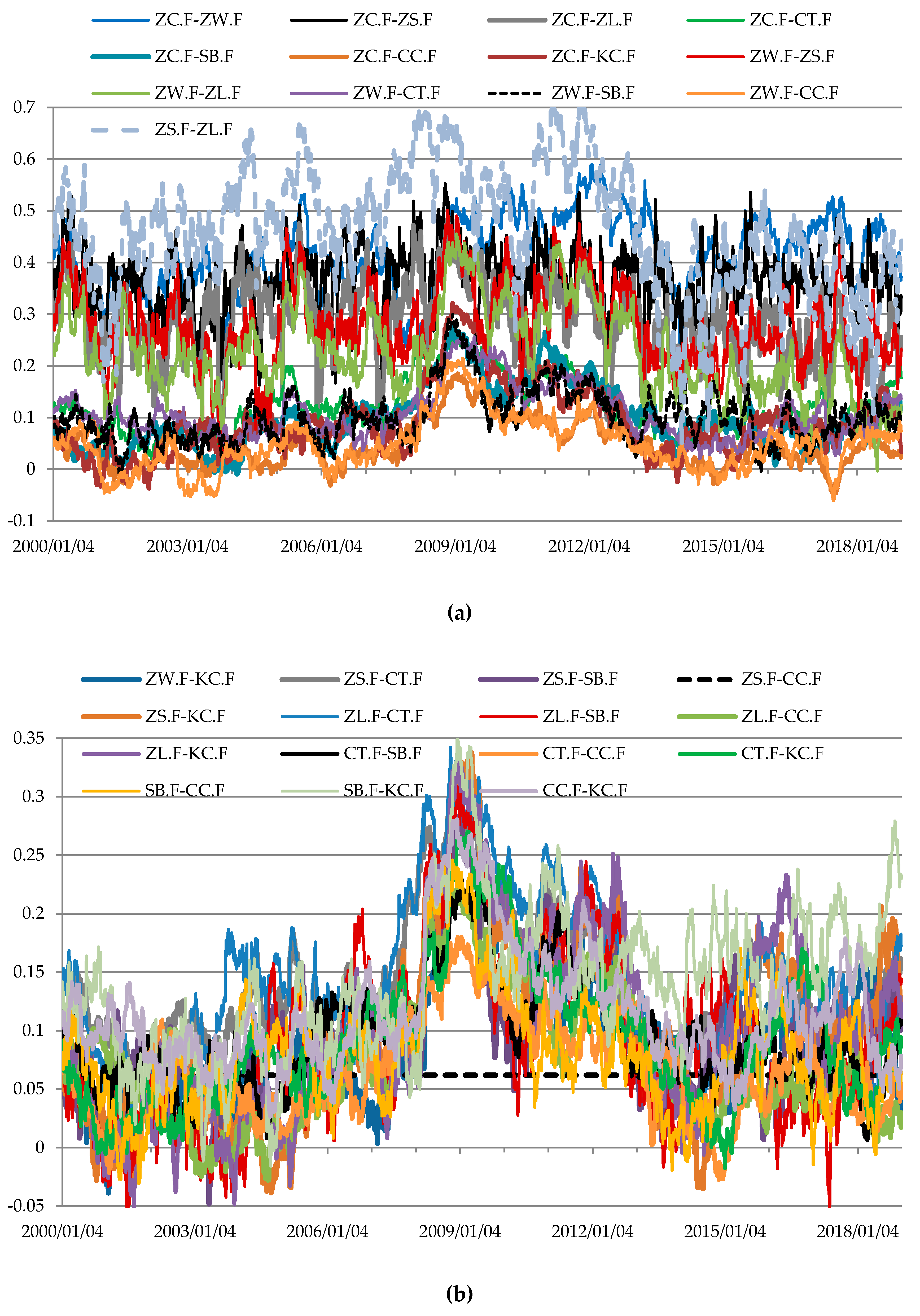
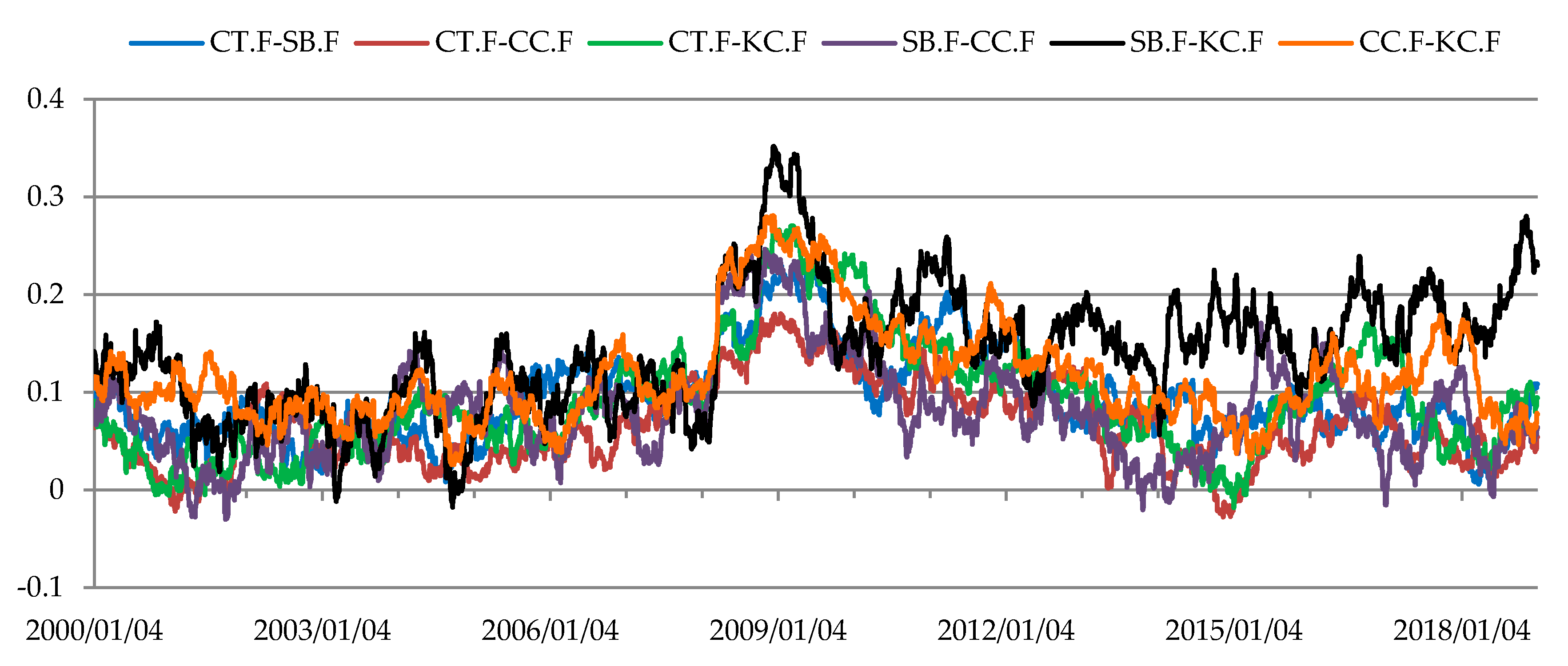
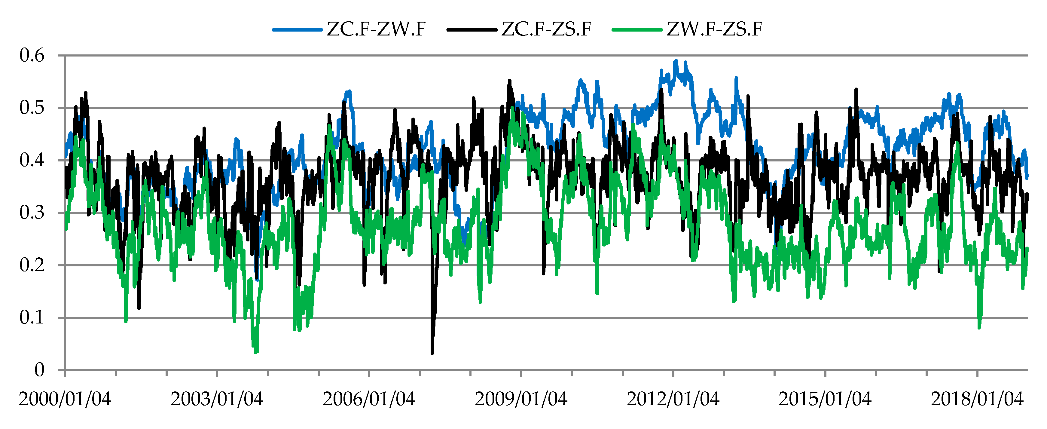
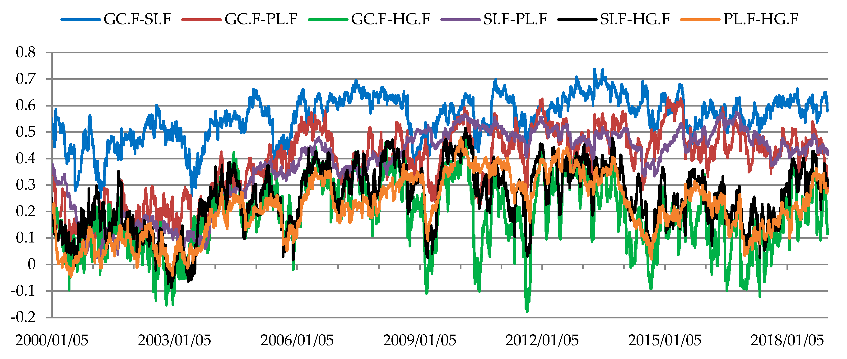
The dynamic Kendall’s tau coefficients were used to assess the strength of conditional dependencies between the returns on prices of commodity futures in the markets for energy, metals, grains and oilseeds, soft commodities and agricultural commodities. The resulting Kendall’s tau coefficients (Figure 1, Figure 2, Figure 3, Figure 4 and Figure 5) were clustered using the fuzzy c-means method (Figure 6, Figure 7, Figure 8, Figure 9 and Figure 10).

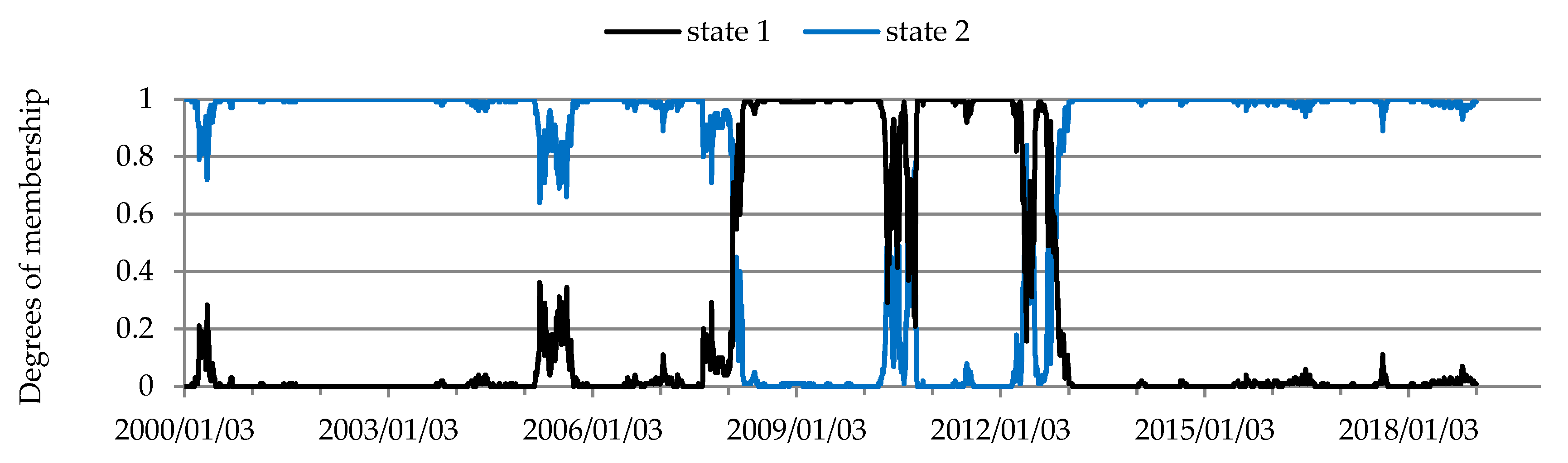
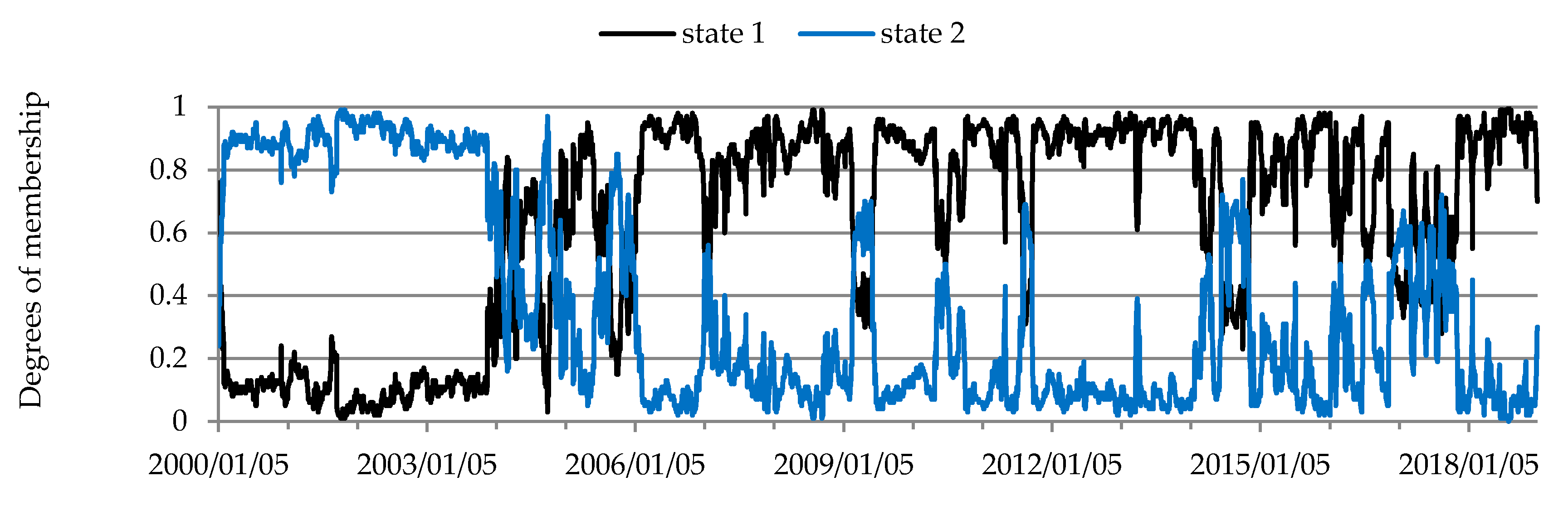
The structure of conditional dependencies in commodity futures markets varied between 2000 and 2018, as confirmed by the different states of markets identified (Figure 6, Figure 7, Figure 8, Figure 9 and Figure 10,

Table 3. Weighted means^* of dynamic Kendall’s tau coefficients for the agricultural futures market.

Specification	ZC.F–ZW.F	ZC.F–ZS.F	ZC.F–ZL.F	ZC.F–CT.F	ZC.F–SB.F	ZC.F–CC.F	ZC.F–KC.F
State 1	0.47	0.39	0.34	0.19	0.18	0.11	0.18
State 2	0.40	0.36	0.27	0.10	0.07	0.03	0.06
Specification	ZW.F–ZS.F	ZW.F–ZL.F	ZW.F–CT.F	ZW.F–SB.F	ZW.F–CC.F	ZW.F–KC.F	ZS.F–ZL.F
State 1	0.35	0.32	0.17	0.16	0.11	0.18	0.58
State 2	0.26	0.19	0.09	0.08	0.03	0.07	0.43
Specification	ZS.F–CT.F	ZS.F–SB.F	ZS.F–CC.F	ZS.F–KC.F	ZL.F–CT.F	ZL.F–SB.F	ZL.F–CC.F
State 1	0.21	0.16	0.06	0.19	0.23	0.18	0.15
State 2	0.11	0.07	0.06	0.07	0.11	0.06	0.05
Specification	ZL.F–KC.F	CT.F–SB.F	CT.F–CC.F	CT.F–KC.F	SB.F–CC.F	SB.F–KC.F	CC.F–KC.F
State 1	0.20	0.15	0.12	0.16	0.13	0.20	0.18
State 2	0.07	0.07	0.05	0.07	0.06	0.12	0.10

^* Weighted means is calculated based on degrees of membership and values of variables.

,

Table 4. Weighted means^* of dynamic Kendall’s tau coefficients for the soft commodities futures market.

Specification	CT.F–SB.F	CT.F–CC.F	CT.F–KC.F	SB.F–CC.F	SB.F–KC.F	CC.F–KC.F
State 1	0.12	0.10	0.14	0.11	0.18	0.16
State 2	0.08	0.05	0.07	0.07	0.13	0.10

^* Weighted means is calculated based on degrees of membership and values of variables.

,

Table 5. Weighted means^* of dynamic Kendall’s tau coefficients for the grains and oilseeds futures market.

Specification	ZC.F–ZW.F	ZC.F–ZS.F	ZW.F–ZS.F
State 1	0.38	0.36	0.27
State 2	0.43	0.37	0.28

^* Weighted means is calculated based on degrees of membership and values of variables.

,

Table 6. Weighted means ^* of dynamic Kendall’s tau coefficients for the metals futures market.

Specification	GC.F–SI.F	GC.F–PL.F	GC.F–HG.F	SI.F–PL.F	SI.F–HG.F	PL.F–HG.F
State 1	0.59	0.44	0.23	0.44	0.30	0.26
State 2	0.51	0.29	0.11	0.28	0.17	0.13

^* Weighted means is calculated based on degrees of membership and values of variables.

and

Table 7. Weighted means ^* of dynamic Kendall’s tau coefficients for the energy futures market.

Specification	HO.F–NG.F	HO.F–CL.F	NG.F–CL.F
State 1	0.30	0.68	0.28
State 2	0.12	0.67	0.11
State 3	0.14	0.47	0.12

^* Weighted means is calculated based on degrees of membership and values of variables.

). In the period from late 2007 to early 2013 marked by the global economic and financial crisis (the 2007–2009 subprime crisis, the 2008–early 2013 European debt crisis), changes in the structure of these dependencies were particularly noticeable in the markets for commodity futures, in which rates of return on quoted prices were generally weakly correlated (soft commodities; agricultural commodities other than grains and oilseeds). As regards futures contracts for agricultural commodities, the strongest dependence between the rates of return was recorded for soybeans and soybean oil futures (Figure 1, Table 3). Soybeans are used in the production of many foods because of their high protein content, with approximately 2/3 of produced soybeans being processed into soybean oil and soybean meal. In turn, soybean oil is used to produce cooking oils, margarine, mayonnaise and salad dressings, in the chemical industry and in biodiesel production [88]. An increase in dependencies between soybeans and soybean oil futures contracts was observed in 2004, with stronger relationships recorded over the next nine years. One of the reasons for the increased dependencies may have been connected with the development of the biofuel market. The requirement to add ethanol to fuels was introduced in 2001 by the European Union and in 2005 by the U.S. Congress [89]. Two states of market were identified in the agricultural commodity futures market (Figure 6, Table 3). The correlation between the rates of return on futures prices in the agricultural commodity market became stronger in early 2008 and remained at a similar level until mid-October, 2012. In approximately the same period stronger dependencies were also recorded in the futures market for soft commodities, where two states of the market were also identified (Figure 7, Table 4).

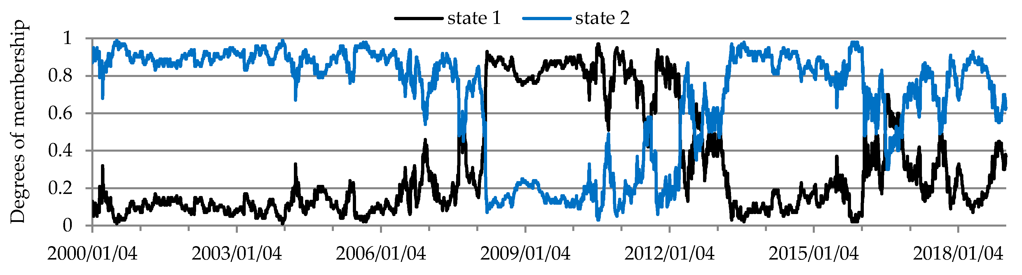
The changes described were not observed in the structure of conditional dependencies between the rates of return on prices of grains and oilseeds futures. In this market two patterns of conditional dependency structure were identified (Figure 8, Table 5). The dependencies between the rates of return on prices of grains and oilseeds futures were moderate or weak. Longer periods of stronger dependencies were recorded from October 2006 to the end of January 2008 and from the end of September 2009 to the end of 2018. In contrast, 2009 saw a decline in the correlation between the rates of return on the analyzed futures (Figure 3), as their prices peaked at record levels at different times, after which they dropped dramatically. The stronger correlations between the rates of return on wheat, corn and soybeans futures in October 2006 were caused by a considerable increase in prices of these futures. During the boom in the market for raw materials, wheat futures prices quadrupled, while corn and soybeans futures prices approximately tripled. The source literature usually lists the following determinants for price growth in the grains and oilseeds market: the development of the biofuel market and the related increase in the correlation between cereals and oilseeds prices and crude oil prices; increased demand caused by economic growth in Asian countries, particularly China; trade liberalization; low stocks of raw materials; underinvestment in agriculture; increase in fertilizer prices; adverse weather conditions; a loose monetary policy (particularly in the US before 2007), which stimulated physical and speculative demand for raw materials; and speculation in the financial markets [5,89,90,91,92,93,94]. The strengthening of dependencies in the futures market for grains and oilseeds is related to an increase in trade volumes in that market. This increase was related to the transition of the Chicago Board of Trade (CBOT) from the open outcry trading system to a new, more efficient online transaction-matching system, as well as the introduction of ETFs and the inflow of capital from financial investors [10]. Opening the market to a broader group of investors resulted in a considerable increase in the number of transactions executed using the online transaction-matching system in the years 2006–2008. According to Irwin and Sanders [10], the enlargement of the group of market players contributed to a decrease in the risk premium and thus reduced hedging costs for raw material producers and processors. In turn, this could also have led to reduced price volatility in commodity markets and the growing integration between commodity and financial markets.

The economic and financial crises (late 2007–early 2013) had no marked impact on the dependency structure in the metal futures market. Two states of the market were identified in the metal futures market (Figure 9, Table 6). The structure of conditional dependencies between the rates of return on prices of metal futures changed in 1Q 2004. Afterwards the rates of return on metal futures were correlated more strongly (Kendall’s tau coefficients increased from approx. 0.1–0.3 to 0.4–0.6), which was particularly evident in the rates of return on the following pairs of futures: platinum–gold and platinum–silver. A relatively strong and stable relationship existed throughout the study period between the rates of return on gold and silver futures (Figure 4, Table 6). The above conclusions are consistent with the findings reported by Sensoy [95], who when analyzing the dynamic conditional correlations in the market of precious metals (gold, silver, platinum and palladium) in the years 1999–2013 found a strong correlation between precious metals in the past decade. This makes diversification less beneficial and indicates a convergence towards one class of assets. When investigating the conditional dependence structure between precious metal rates of return, Wanat et al. [39] also recorded a change on April 29, 2004. Since this study applied the fuzzy c-means method, when analyzing the degrees of membership of moments (days) to the identified states of the market it may be clearly seen that the period of transition from one state of the market to another in the metal futures market was longer and lasted two years (2004–2005). In those years the correlation between the rates of return on metal futures was increasing. Additionally, it was also a period marked by a considerable rise in metal futures prices. These findings do not corroborate the general observation that in the financial markets the dependencies between assets tend to become stronger in periods of declining prices [96]. Conversely, our results are consistent with those reported by Attaf et al. [12], who when studying the period 1960–April 2014 found stronger relationships between most analyzed spot markets for non-energy commodities (metals and minerals, fats and oils, grains, other foods, beverages, agricultural raw materials) during periods of price increases in those markets.

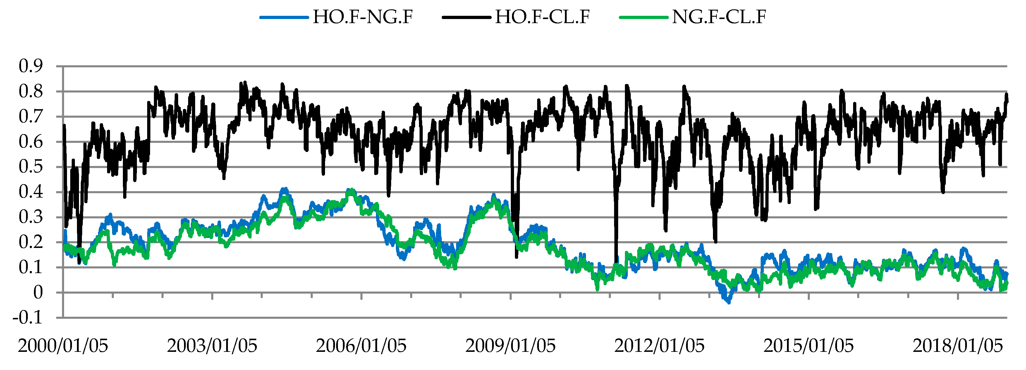
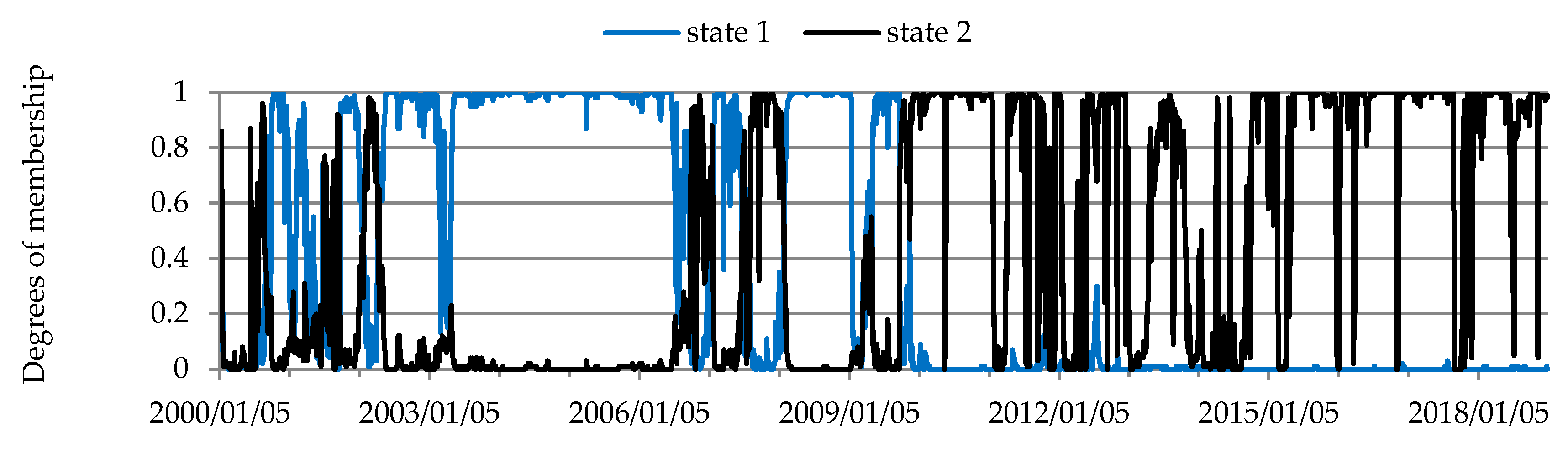
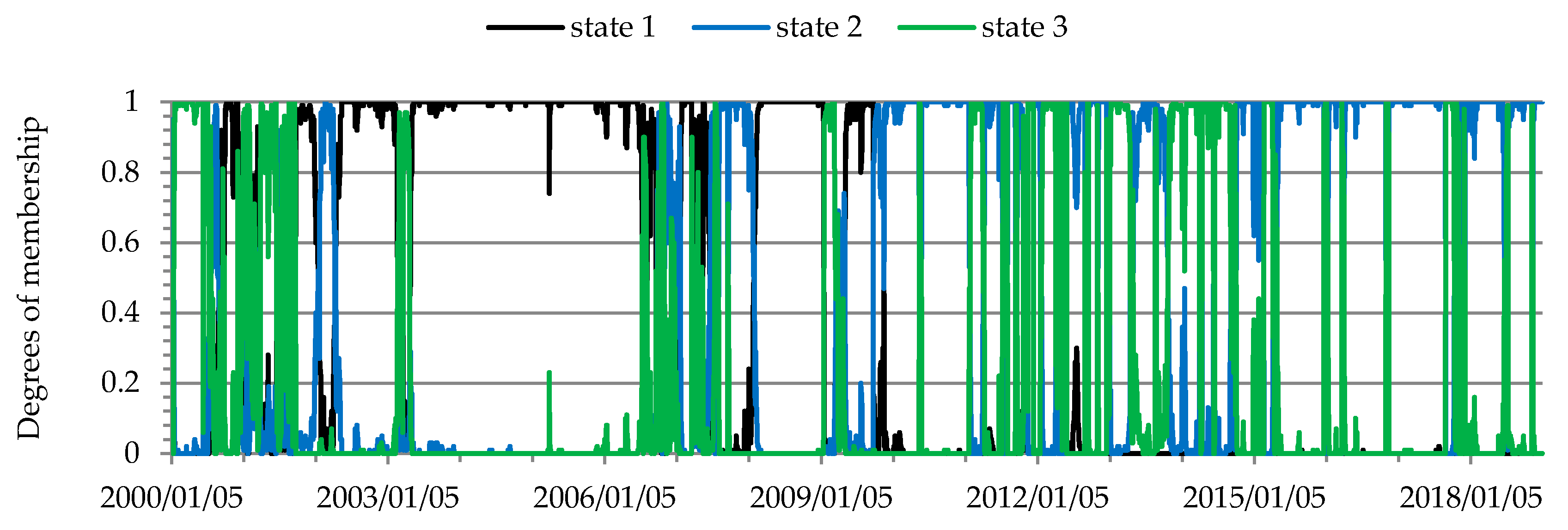
Three patterns of conditional dependency structures were identified in the energy futures market (Figure 10, Table 7). The structure of conditional dependencies underwent a major change in early 2Q 2002 and next in April 2003. Between then and mid-2006 the correlation between the rates of return on energy futures prices was greater than in the other periods. During most of the above-mentioned period contract prices followed an upward trend. This was caused by a sharp rise in crude oil prices, which began in March 2003 following the invasion of Iraq. Global economic growth is believed to be the main cause for the increase in crude oil prices in the years 2003–2008 [97]. During the suprime crisis (February 2008–January 2009) also, the energy futures market was in the state characterized by the highest level of correlation. A strong and relatively stable relationship existed between the rates of return on crude oil and heating oil futures (Figure 5, Table 7). That relationship was caused by links between these basic commodities (heating oil is produced by the distillation of crude oil).

Based on these findings it may be concluded that very weak correlations existed between the rates of return on prices of most futures in the markets for agricultural commodities and soft commodities. Conversely, moderate or strong and relatively stable relationships were found between rates of return on futures on fundamentally interrelated commodities (i.e., commodities which are substitutes or raw materials used to produce other commodities) (Figure 1, Figure 2, Figure 3, Figure 4 and Figure 5, Table 3, Table 4, Table 5, Table 6 and Table 7).

4. Conclusions

The use of copula-GARCH models and fuzzy clustering methods in assessing the structure of dependencies in five selected markets for commodity futures (agricultural commodities, soft commodities, grains and oilseeds, metals, energy) in the years 2000–2018 allowed the formulation of the following conclusions. In all commodity futures markets the structure of conditional dependencies changed over the study period. Two states of the market (corresponding to typical patterns of conditional dependency structures) were identified in the markets for agricultural commodities, soft commodities, grains and oilseeds and metals, while three states of market were identified in the energy market. The strongest (and relatively stable) conditional dependencies existed between the rates of return on futures contracts on commodities which are linked with a substitution relationship or are raw materials used to manufacture other commodities (i.e., crude oil—heating oil; gold—silver, soybeans—soybean oil). In turn, during the economic and financial crises (late 2007–early 2013), a marked change in the structure of conditional dependencies was particularly evident in the futures markets for soft commodities, agricultural commodities and energy. However, it needs to be remembered that following an increase in late 2007–early 2008, the correlation between the rates of return on prices of most futures traded in the markets for soft commodities and agricultural commodities continued to be weak. This means that portfolios composed of futures listed in these two markets were well diversified and the turbulence affecting those markets did not lead to any significant risk increase for those portfolios. The dependencies were stronger in the futures markets for grains and oilseeds, as well as metals and energy. In the grains and oilseeds futures market stronger correlations were found in the two sub-periods: from October 2006 until the end of January 2008 and from the end of September 2009 until the end of 2018. A major shift in the conditional dependence structure in the metal futures market (towards a greater correlation between the rates of return) took place in 1Q 2004. In turn, the energy futures market experienced a longer period of stronger dependencies, which included two sub-periods: from the beginning of 2Q 2002 until the end of 1H 2006, and from February 2008 until mid-January 2009.

The analysis of the structure of conditional dependencies in the markets for commodity futures provides insight into the stability of conditional dependencies in commodity markets. The findings from this study may be useful to investors and portfolio managers in the risk management process. This information also may provide some implications for policy makers and participants in commodity markets.

A limitation in this study was connected with a lack of a synthetic measure, which would determine dependencies between all market contracts at individual moments (days) or periods corresponding to specific states of the market. The analysis presented in this paper shows that the correlations between commodity futures vary significantly. This phenomenon may result in numerous problems when constructing well diversified portfolios. Using a single aggregated value of correlation for all pairs of contracts instead of their actual values the investors could build more stable portfolios. Elton and Gruber [98] and Ledoit and Wolf [99] demonstrated that using a “mean” correlation helps in selecting a portfolio which is less volatile than those based on pair-wise correlations. Therefore, the next step of this research will consist in constructing a synthetic measure, which using a single number would determine the relationships between all assets in the market at individual moments or states of the market. Further research will focus on analyzing the effect of the diversification of investment portfolios with the use of a dynamic synthetic measure. Another direction for future studies will concern the analysis of dependencies between extreme values recorded in commodity futures markets. The analysis of extreme dependencies is of particular importance to investors and managers of portfolios composed of commodities or commodity futures, since prices of many commodities rise as a consequence of shocks generated by catastrophic events (e.g. drought, war).

References

- Markowitz, H. Portfolio selection. J. Financ. 1952, 7, 77–91. [Google Scholar]
- Satyanarayan, S.; Varangis, P. An Efficient Frontier for International Portfolios with Commodity Assets; Policy Research Working Paper WPS 1266; World Bank: Washington, DC, USA, 1994; Available online: http://documents.worldbank.org/curated/en/487921468766163574/pdf/multi-page.pdf (accessed on 5 December 2019).
- Greer, R. The nature of commodity index returns. J. Altern. Invest. 2000, 3, 45–52. [Google Scholar] [CrossRef]
- Gorton, G.; Rouwenhorst, K.G. Facts and Fantasies about Commodity Futures; Working Paper 10595; National Bureau of Economic Research (NBER): Cambridge, MA, USA, 2004; Available online: http://www.nber.org/papers/w10595.pdf (accessed on 5 December 2019).
- Inamura, Y.; Kimata, T.; Kimura, T.; Muto, T. Recent surge in global commodity prices—Impact of financialization of commodities and globally accommodative monetary conditions. Bank Jpn. Rev. 2011, E2. Available online: https://www.boj.or.jp/en/research/wps_rev/rev_2011/data/rev11e02.pdf (accessed on 5 December 2019).
- Bodie, Z.; Rosansky, V.I. Risk and return in commodity futures. Financ. Anal. J. 1980, 36, 27–39. [Google Scholar] [CrossRef]
- Jaffe, J.F. Gold and gold stocks as investments for institutional portfolios. Financ. Anal. J. 1989, 45, 53–59. [Google Scholar] [CrossRef]
- Froot, K.A. Hedging portfolios with real assets. J. Port. Manag. 1995, 21, 60–77. [Google Scholar] [CrossRef]
- Jensen, G.R.; Johnson, R.R.; Mercer, J.M. Efficient use of commodity futures in diversified portfolios. J. Futur. Mark. 2000, 20, 489–506. [Google Scholar] [CrossRef]
- Irwin, S.H.; Sanders, D.R. Financialization and structural change in commodity futures markets. J. Agric. Appl. Econ. 2012, 44, 371–396. [Google Scholar] [CrossRef] [Green Version]
- Tang, K.W.; Xiong, W. Index investment and financialization of commodities. Financ. Anal. J. 2012, 68, 54–74. [Google Scholar] [CrossRef]
- Attaf, Z.; Ghorbel, A.; Boujelbène, Y. Dependence between non-energy commodity sectors using time-varying extreme value copula methods. Int. J. Econ. Financ. Manag. 2015, 3, 64–75. [Google Scholar]
- Putnam, K.J. Two Essays in Financial Economics; University of New Orleans: New Orleans, LA, USA, 2015; Available online: https://scholarworks.uno.edu/td/2010 (accessed on 4 November 2019).
- Zaremba, A. Inflation, business cycles, and commodity investing in financialized markets. Bus. Econ. Res. J. 2015, 6, 1–18. [Google Scholar]
- Han, X.; Liu, Z.; Wang, S. Tail dependence structure of metal commodity futures in London metal exchange. In Proceedings of the EFMA Annual Meetings, Ponta Delgada, Portugal, 26–29 June 2019; University of Azores: Ponta Delgada, Portugal, 2019. Available online: https://efmaefm.org/0EFMAMEETINGS/EFMA%20ANNUAL%20MEETINGS/2019-Azores/papers/EFMA2019_0052_fullpaper.pdf (accessed on 24 October 2019).
- Andersen, T.G.; Bollerslev, T.; Diebold, F.X.; Labys, P. Understanding, Optimizing, Using and Forecasting Realized Volatility and Correlation; Northwestern University: Evanston, IL, USA; Duke University: Durham, NC, USA; University of Pennsylvania: Philadelphia, PA, USA, 1999; Available online: https://www.sas.upenn.edu/~fdiebold/papers/paper29/temp.pdf (accessed on 10 October 2019).
- Liu, J. A New Tail-Based Correlation Measure and Its Application in Global Equity Markets; Policy Research Working Paper WPS 8709; World Bank Group: Washington, DC, USA, 2019; Available online: http://documents.worldbank.org/curated/en/641081547753593928/pdf/WPS8709.pdf (accessed on 5 December 2019).
- McNeil, A.J.; Frey, R.; Embrechts, P. Quantitative Risk Management: Concepts, Techniques and Tools; Princeton University Press: Princeton, NJ, USA, 2005. [Google Scholar]
- Bauwens, L.; Laurent, S.; Rombouts, J.V.K. Multivariate GARCH models: A survey. J. Appl. Econ. 2006, 21, 79–109. [Google Scholar] [CrossRef] [Green Version]
- Engle, R.F. Dynamic conditional correlation: A simple class of multivariate GARCH models. J. Bus. Econ. Stat. 2002, 20, 339–350. [Google Scholar] [CrossRef]
- Patton, A.J. Copula-Based models for financial time series. In Handbook of Financial Time Series; Andersen, T.G., Davis, R.A., Kreiss, J.-P., Mikosch, T., Eds.; Springer: New York, NY, USA, 2009; pp. 767–786. [Google Scholar]
- Doman, M.; Doman, R. Dynamics of Dependencies on the Global Financial Market; Difin: Warsaw, Poland, 2014. (In Polish) [Google Scholar]
- Jondeau, E.; Rockinger, M. The Copula-GARCH model of conditional dependencies: An international stock market application. J. Int. Money Financ. 2006, 25, 827–853. [Google Scholar] [CrossRef] [Green Version]
- Engle, R.; Kelly, B. Dynamic equicorrelation. J. Bus. Econ. Stat. 2012, 30, 212–228. [Google Scholar] [CrossRef]
- Chicago Board Options Exchange. CBOE S&P 500 Implied Correlation Index. 2009. Available online: https://www.cboe.com/micro/impliedcorrelation/impliedcorrelationindicator.pdf (accessed on 25 July 2018).
- Cambell, R.; Koedijk, K.; Kofman, P. Increased correlation in bear markets. Financ. Anal. J. 2002, 58, 87–94. [Google Scholar] [CrossRef]
- Echaust, K.; Just, M. Implied correlation index: An application to economic sectors of commodity futures and stock markets. Inz. Ekon. Eng. Econ. 2020, 31, 4–17. [Google Scholar] [CrossRef] [Green Version]
- Bachman, D.; Choi, J.J.; Jeon, B.; Kopecky, K. Common factors in international stock prices: Evidence from a cointegration study. Int. Rev. Financ. Anal. 1996, 5, 39–53. [Google Scholar] [CrossRef]
- Ciner, C. On the long run relationship between gold and silver prices: A note. Glob. Financ. J. 2001, 12, 299–303. [Google Scholar] [CrossRef]
- Nazlioglu, S. World oil and agricultural commodity prices: Evidence from nonlinear causality. Energy Policy 2011, 39, 2935–2943. [Google Scholar] [CrossRef]
- Nazlioglu, S.; Soytas, U. Oil price, agricultural commodity prices, and the dollar: A panel cointegration and causality analysis. Energy Econ. 2012, 34, 1098–1104. [Google Scholar] [CrossRef]
- Fernandez, V. Linear and non-linear causality between price indices and commodity prices. Resour. Policy 2014, 41, 40–51. [Google Scholar] [CrossRef]
- Giot, P.; Laurent, S. Market risk in commodity markets: A VaR approach. Energy Econ. 2003, 25, 435–457. [Google Scholar] [CrossRef]
- Marimoutou, V.; Raggad, B.; Trabelsi, A. Extreme value theory and value at risk: Application to oil. Energy Econ. 2009, 31, 519–530. [Google Scholar] [CrossRef] [Green Version]
- Cheng, W.-H.; Hung, J.-C. Skewness and leptokurtosis in GARCH-typed VaR estimation of petroleum and metal asset returns. J. Empir. Financ. 2011, 18, 160–173. [Google Scholar] [CrossRef]
- Morgan, W.; Cotter, J.; Dowd, K. Extreme measure of agricultural risk. J. Agric. Econ. 2012, 63, 65–82. [Google Scholar] [CrossRef] [Green Version]
- Van Oordt, M.R.C.; Stork, P.A.; de Vries, C. On Agricultural Commodities’ Extreme Price Risk; DNB Working Paper 403; De Nederlandsche Bank: Amsterdam, The Netherlands, 2013; Available online: https://papers.ssrn.com/sol3/papers.cfm?abstract_id=2362305 (accessed on 5 December 2019).
- Just, M. The use of value-at-risk models to estimate the investment risk on agricultural commodity market. In Proceedings of the International Conference Hradec Economic Days 2014: Economic Development and Management of Regions, Hradec Králové, Czech Republic, 3–4 February 2014; Jedlička, P., Ed.; University Hradec Králové: Hradec Králové, Czech Republic, 2014; Volume 4, pp. 264–273. [Google Scholar]
- Wanat, S.; Papież, M.; Śmiech, S. The conditional dependence structure between precious metals: A Copula-GARCH approach. Crac. Rev. Econ. Manag. 2015, 4, 19–33. [Google Scholar] [CrossRef] [Green Version]
- Aepli, M.D.; Füss, R.; Henriksen, T.E.S.; Paraschiv, F. Modeling the multivariate dynamic dependence structure of commodity futures portfolios. J. Commod. Mark. 2017, 6, 66–87. [Google Scholar] [CrossRef] [Green Version]
- Yamaka, W.; Phadkantha, R.; Sriboonchitta, S. Modeling dependence of agricultural commodity futures through Markov switching copula with mixture distribution regimes. Thai J. Math. 2019, Spec. Issue Struct. Chang. Model. Optim. Econom. 2018, 17, 93–107. [Google Scholar]
- Bollerslev, T. Generalized autoregressive conditional heteroskedasticity. J. Econ. 1986, 31, 307–327. [Google Scholar] [CrossRef] [Green Version]
- Taylor, S.J. Modelling Financial Time Series; John Wiley & Sons: Chichester, UK, 1986. [Google Scholar]
- Schwert, G.W. Stock volatility and the crash of ‘87. Rev. Financ. Stud. 1990, 3, 77–102. [Google Scholar] [CrossRef] [Green Version]
- Nelson, D.B. Conditional heteroskedasticity in asset returns: A new approach. Econometrica 1991, 59, 347–370. [Google Scholar] [CrossRef]
- Bollerslev, T.; Mikkelsen, H.O. Modeling and pricing long-memory in stock market volatility. J. Econ. 1996, 73, 151–184. [Google Scholar] [CrossRef]
- Glosten, L.R.; Jagannathan, R.; Runkle, D.E. On the relation between the expected value and the volatility of the nominal excess return on stocks. J. Financ. 1993, 48, 1779–1801. [Google Scholar] [CrossRef]
- Ding, Z.; Granger, C.W.J.; Engle, R.F. A long memory property of stock market returns and a new model. J. Empir. Financ. 1993, 1, 83–106. [Google Scholar] [CrossRef]
- Zakoian, J.M. Threshold heteroskedastic models. J. Econ. Dyn. Control 1994, 18, 931–955. [Google Scholar] [CrossRef]
- Baillie, R.T.; Bollerslev, T.; Mikkelsen, H.O. Fractionally integrated generalized autoregressive conditional heteroskedasticity. J. Econ. 1996, 74, 3–30. [Google Scholar] [CrossRef]
- Delatte, A.-L.; Lopez, L. Commodity and equity markets: Some stylized facts from a copula approach. J. Bank. Financ. 2013, 37, 5346–5356. [Google Scholar] [CrossRef] [Green Version]
- Just, M.; Łuczak, A.; Kozera, A. Conditional dependence structure in the precious metals futures market. Int. J. Econ. Sci. 2019, 8, 81–93. [Google Scholar] [CrossRef]
- Acworth, W. 2015 Annual Survey: Global Derivatives Volume. MarketVoice, FIA’s Magazine of the Global Futures, Options and Cleared Swaps Mark. 2016. Available online: http://www.marketvoicemag.org/?q=content/2015-annual-survey-global-derivatives-volume (accessed on 6 September 2016).
- FIA Releases Annual Trading Statistics Showing Record ETD Volume in 2018. Available online: https://fia.org/articles/fia-releases-annual-trading-statistics-showing-record-etd-volume-2018 (accessed on 22 August 2019).
- Financial Stock News. Available online: https://www.stooq.pl (accessed on 4 March 2019).
- Tsay, R.S. Analysis of Financial Time Series; John Wiley & Sons: New York, NY, USA, 2005. [Google Scholar]
- Hansen, P.R.; Lunde, A. A forecast comparison of volatility models: Does anything beat a GARCH (1, 1)? J. Appl. Econ. 2005, 20, 873–889. [Google Scholar] [CrossRef] [Green Version]
- Bollerslev, T. Modeling the coherence in short-run nominal exchange rates: A multivariate generalized ARCH model. Rev. Econ. Stat. 1990, 72, 498–505. [Google Scholar] [CrossRef]
- Ghalanos, A. Rmgarch: Multivariate GARCH Models. R Packages, Version 1.3-0. 2015. Available online: https://mran.microsoft.com/snapshot/2016-10-12/web/packages/rmgarch/index.html (accessed on 15 March 2018).
- Ghalanos, A. Rugach: Univariate GARCH Models. R Package, Version 1.4-0. 2018. Available online: https://cran.r-project.org/web/packages/rugarch/index.html (accessed on 31 January 2019).
- Hartigan, J.A. Clustering Algorithms; John Wiley & Sons: New York, NY, USA, 1975. [Google Scholar]
- Zadeh, L.A. Fuzzy sets. Inf. Control 1965, 8, 338–353. [Google Scholar] [CrossRef] [Green Version]
- Grabiński, T. Methody of Taxonometry; Cracow Academy of Economics: Cracow, Poland, 1992. (In Polish) [Google Scholar]
- Wysocki, F. Methods of Statistical Multidimensional Analysis in Recognizing the Types of Spatial Structure of Agriculture; August Cieszkowski Agricultural University: Poznan, Poland, 1996. (In Polish) [Google Scholar]
- Wysocki, F. The Methods of Taxonomy for Recognition of Economic Types in Agriculture and Rural Areas; Poznań University of Life Sciences: Poznan, Poland, 2010. (In Polish) [Google Scholar]
- Kim, T.; Bezdek, J.C.; Hathaway, R.J. Optimality tests for fixed points of the fuzzy c-means algorithm. Pattern Recognit. 1988, 21, 651–663. [Google Scholar] [CrossRef]
- Digby, P.G.N.; Gower, J.C. Ordination and Classification; Les Presses de l’Université de Montréal: Montreal, QC, Canada, 1986. [Google Scholar]
- Jain, A.K.; Moreau, J.V. Bootstrap technique in cluster analysis. Pattern Recognit. 1987, 20, 547–568. [Google Scholar] [CrossRef]
- Jajuga, K. Multivariate Statistical Analysis; Polish Scientific Publishers PWN: Warsaw, Poland, 1993. (In Polish) [Google Scholar]
- Kamel, M.S.; Selim, S.Z. A relaxation approach to the fuzzy clustering problem. Fuzzy Sets Syst. 1994, 61, 177–188. [Google Scholar] [CrossRef]
- Höppner, F.; Klawonn, F.; Kruse, R.; Runkler, T. Fuzzy Cluster Analysis: Methods for Classification, Data Analysis and Image Recognition; John Wiley & Sons: Chichester, UK, 1999. [Google Scholar]
- Milligan, G.W.; Cooper, M.C. An examination of procedures for determining the number of clusters in a data set. Psychometrika 1985, 2, 159–179. [Google Scholar] [CrossRef]
- Fischer, A. On the number of groups in clustering. Stat. Probab. Lett. 2011, 81, 1771–1781. [Google Scholar] [CrossRef]
- Caliński, R.B.; Harabasz, J. A dendrite method for cluster analysis. Commun. Stat. 1974, 3, 1–27. [Google Scholar]
- Baker, F.; Hubert, L. Measuring the power of hierarchical cluster analysis. J. Am. Stat. Assoc. 1975, 70, 31–38. [Google Scholar] [CrossRef]
- Hubert, L.; Levin, J. A general statistical framework for assessing categorical clustering in free recall. Psychol. Bull. 1976, 83, 1072–1080. [Google Scholar] [CrossRef]
- Krzanowski, W.J.; Lai, Y.T. A criterion for determining the number of clusters in a data set. Biometrics 1985, 44, 23–34. [Google Scholar] [CrossRef]
- Kaufman, L.; Rousseeuw, P. Finding Groups in Data: An Introduction to Cluster Analysis; John Wiley & Sons: New York, NY, USA, 1990. [Google Scholar]
- Tibshirani, R.; Walther, G.; Hastie, T. Estimating the number of clusters in a data set via the gap statistic. J. R. Stat. Soc. Ser. B 2001, 63, 411–423. [Google Scholar] [CrossRef]
- Bezdek, J.C. Fuzzy Mathematics in Pattern Classification. Ph.D. Thesis, Cornell University, Ithaca, NY, USA, 1973. [Google Scholar]
- Bezdek, J.C. Pattern Recognition with Fuzzy Objective Function Algorithms; Plenum Press: New York, NY, USA, 1981. [Google Scholar]
- Pal, N.R.; Bezdek, J.C. On cluster validity for the fuzzy c-means model. IEEE Trans. Fuzzy Syst. 1995, 3, 370–379. [Google Scholar] [CrossRef]
- Pal, N.R.; Bezdek, J.C. Correction to “on cluster validity for the fuzzy c-means model”. IEEE Trans. Fuzzy Syst. 1997, 1, 152–153. [Google Scholar] [CrossRef]
- Dunn, J.C. A fuzzy relative of ISODATA process and its use in detecting compact well-separated cluster. J. Cybern. 1973, 3, 32–57. [Google Scholar] [CrossRef]
- Łuczak, A.; Wysocki, F. Applications of Taxonometric Methods and Analytic Hierarchy Process to Programming of Development of Rural Areas; August Cieszkowski Agricultural University: Poznan, Poland, 2005. (In Polish) [Google Scholar]
- Walesiak, M.; Dudek, A. ClusterSim: Searching for Optimal Clustering Procedure for a Data Set, R Package Version 0.47-1. 2017. Available online: https://cran.r-project.org/web/packages/clusterSim (accessed on 24 July 2018).
- Giordani, P.; Ferraro, M.B.; Serafini, A. Fclust: Fuzzy Clustering, R package. 2018. Available online: https://cran.r-project.org/web/packages/fclust (accessed on 13 March 2019).
- CME Group. Available online: https://www.cmegroup.com (accessed on 11 February 2019).
- Świerczyńska, U. Causes of the global food crisis and its impact on the poorest countries in the Word. In Global Warming and Food Crisis; Wilk, W., Ed.; The Polish Center for International Aid: Warsaw, Poland, 2008; pp. 33–45. (In Polish) [Google Scholar]
- Conley, D.M.; George, A. Spatial marketing patterns for corn under the condition of increasing ethanol production in the U.S. Int. Food Agribus. Manag. Rev. 2008, 11, 81–98. [Google Scholar]
- Mayer, J. The Growing Interdependence between Financial and Commodity Markets; UNCTAD Discussion Papers 195; United Nations Conference on Trade and Development (UNCTAD): Geneva, Switzerland, 2009; Available online: http://unctad.org/en/docs/osgdp20093_en.pdf (accessed on 5 December 2019).
- Cooke, B.; Robles, L. Recent Food Prices Movements: A Time Series Analysis; IFPRI Discussion Paper 00942; International Food Policy Research Institute (IFRI): Washington, DC, USA, 2009; Available online: http://www.ifpri.org/publication/recent-food-prices-movements (accessed on 5 December 2019).
- Gilbert, C.L. How to understand high food prices. J. Agric. Econ. 2010, 61, 398–425. [Google Scholar] [CrossRef]
- Abbott, P.; Borot de Battisti, A. Recent global food price shocks: Causes, consequences and lessons for African governments and donors. J. Afr. Econ. 2011, 20, i12–i62. [Google Scholar] [CrossRef]
- Sensoy, A. Dynamic relationship between precious metals. Resour. Policy 2013, 38, 504–511. [Google Scholar] [CrossRef]
- Longin, F.; Solnik, B. Extreme correlation of international equity markets. J. Financ. 2001, 56, 649–676. [Google Scholar] [CrossRef]
- Grudziński, Z. Relations of energy commodity prices on world markets. Min. Rev. 2009, 65, 9–14. (In Polish) [Google Scholar]
- Elton, E.J.; Gruber, M.J. Estimating the dependence structure of share prices—Implications for portfolio selection. J. Financ. 1973, 28, 1203–1232. [Google Scholar]
- Ledoit, O.; Wolf, M. Improved estimation of the covariance matrix of stock returns with an application to portfolio selection. J. Empir. Financ. 2003, 10, 603–621. [Google Scholar] [CrossRef] [Green Version]
Figure 1.
(a) Estimates of dynamic Kendall’s tau coefficients for dependencies between rates of return from futures for agricultural commodities. (b) Estimates of dynamic Kendall’s tau coefficients for dependencies between rates of return from futures for agricultural commodities.
Figure 2.
Estimates of the dynamic Kendall’s tau coefficients for dependencies between rates of return from futures for soft commodities.
Figure 3.
Estimates of the dynamic Kendall’s tau coefficients for dependencies between rates of return from futures for grains and oilseeds.
Figure 4.
Estimates of the dynamic Kendall’s tau coefficients for dependencies between rates of return from futures for metals.
Figure 5.
Estimates of the dynamic Kendall’s tau coefficients for dependencies between rates of return from futures for energy.
Figure 6.
Temporal evolution of the state of the futures market for agricultural commodities.
Figure 7.
Temporal evolution of the state of the futures market for soft commodities.
Figure 8.
Temporal evolution of the state of the grains and oilseeds futures market.
Figure 9.
Temporal evolution of the state of the metals futures market.
Figure 10.
Temporal evolution of the state of the energy futures market.