Variation in Phytoplankton Community Due to an Autumn Typhoon and Winter Water Turbulence in Southern Korean Coastal Waters

Abstract

We evaluated changes in the phytoplankton community in Korean coastal waters during October 2016 and February 2017. Typhoon Chaba introduced a large amount of freshwater into the coastal areas during autumn 2016, and there was a significant negative relationship between salinity and nutrients in the Nakdong estuarine area, particularly in the northeastern area (Zone III; p < 0.001). The abundance of diatom species, mainly Chaetoceros spp., increased after this nutrient loading, whereas Cryptomonas spp. appeared as opportunists when there was relatively low diatom biomass. During winter, biotic and abiotic factors did not differ among the surface, middle, and lower layers (p > 0.01; ANOVA), implying that water mixing by winter windstorms and low surface temperature (due to the sinking of high-density water) physically accelerated mixing of the whole water column. Diatoms predominated under these conditions. Among diatoms, the centric diatom Eucampia zodiacus remained at high density at the inshore area and its abundance had a negative correlation with water temperature, implying that this species can grow at cold temperatures. On the other hand, the harmful freshwater diatom Stephanodiscus hantzschii mainly appeared in conditions with low salinity and high nutrients, implying that it can persist even in the saltwater conditions of the Nakdong Estuary. Our results indicate that hydro-oceanographic characteristics, such as river discharge after an autumn typhoon and winter water turbulence, have major effects on the composition of phytoplankton communities and can potentially affect the occurrence and characteristics of harmful algal blooms in southern Korean coastal waters.

1. Introduction

The seasonal phytoplankton bloom cycle and species succession that occur in temperate seas are influenced by environmental bottom-up control factors, such as temperature, light availability, and nutrient loading, and by top-down control factors, such as zooplankton grazing [1,2]. The supply of limiting nutrients has a major impact on phytoplankton composition and abundance, and this depends on species-specific differences in nutrient uptake. In addition, the growth of phytoplankton is often limited by one or more essential nutrients [3,4,5]. Overall, phytoplankton blooms can be partially explained by the distribution of nutrients within the water mass [6]. In particular, a sudden supply of nutrients from river discharge after rainfall and nutrient supplementation of euphotic layers by upwelling and turbulence caused by episodic wind typically promote phytoplankton growth in coastal environments [7,8,9].

In coastal regions, nearby typhoons often cause physical disturbances, such as upwelling, vertical mixing, terrestrial runoff, and sediment resuspension, and these supply nutrients directly to the euphotic layer [10,11]. In addition, during winter months, windstorms can cause significant water mixing and increase nutrient loading in the whole water column, which is continuously accumulated to the euphotic layer due to the reduced phytoplankton nutrient uptake caused by the lower levels of light and shorter photoperiods during winter in temperate coastal waters. Therefore, the increased nutrient loading caused by such events significantly affects the population dynamics and coastal distribution patterns of phytoplankton [12,13].

In the coastal waters of the southern part of Korea (such as Tongyeong, Geoje, and Busan), the physical water mass during the autumn and winter seasons is more strongly affected by the Jeju Warm Current and Tsushima Warm Current (TWC), both of which originate from the Kuroshio Warm Current (Figure 1a) [14,15,16]. The Tongyeong, Geoje, and Busan coastal areas, which are near the Kahwa Estuary and the Nakdong River Estuary, are located along the southeastern Korean Peninsula (Figure 1b). Numerous bivalve mollusks (oysters and ark shells) and fish farms have been established in these coastal areas. These aquaculture activities have led to the accumulation of organic matter in sediments, and this organic matter is one of the major non-point nutrient sources in these coastal waters. The Nakdong River is Korea’s longest river and the Nakdong Estuary is Korea’s second largest estuary [17]. In addition, the Nakdong Estuary neighbors the city of Busan, which has a population of about 4 million.

Seasonal monsoons strongly affect the climate of the Korean Peninsula. Relatively weak south to southeasterly winds and heavy precipitation are typical during the summer monsoon, and increased discharge from the Nakdong River, caused by summer-autumn typhoons, significantly affects the Busan and Geoje coastal waters. On the other hand, strong north to northwesterly winds and minimal precipitation are common during winter.

The present study examined the effect of Typhoon Chaba (autumn 2016) and the subsequent winter water turbulence (winter 2017) on southern Korean coastal waters and the responses of the phytoplankton communities in this region. In particular, we examined the effects of these two major events on changes in multiple environmental variables, phytoplankton abundance, and phytoplankton composition.

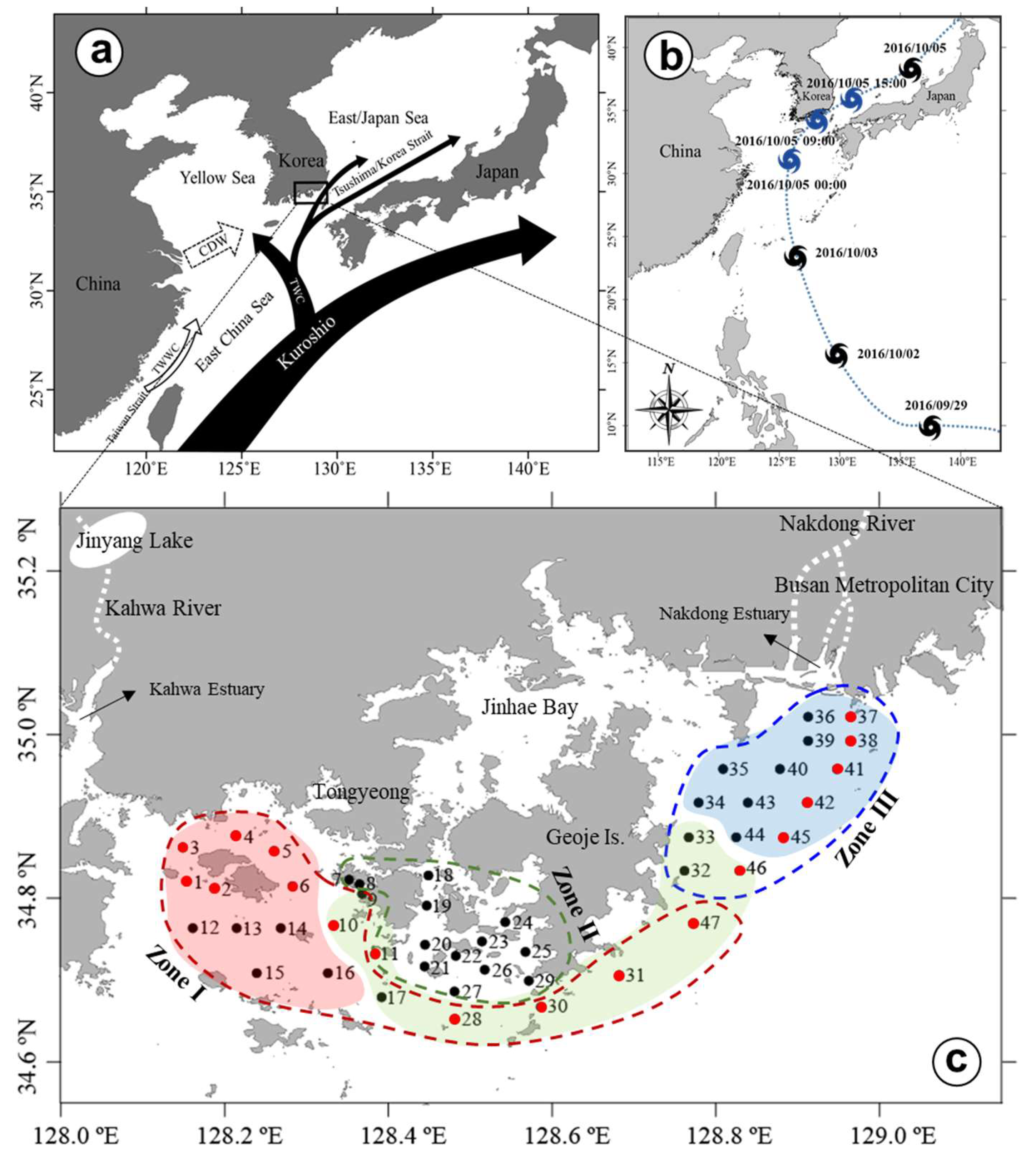
2. Materials and Methods

2.1. Field Sampling and Analysis

The present study was a field survey performed during autumn (18 to 19 October 2016) and winter (6 to 7 February 2017) on board the R/V Jangmok I. A total of 47 stations along the Busan, Geoje, and Tongyeong coast were established on the inner and outer coastal waters, including two major rivers—the Kahwa and Nakdong Estuaries (Figure 1b). Water samples at all of the stations were collected from the surface and bottom layers using a 5-L polyvinyl chloride Niskin sampler (General Oceanics, Miami, FL, USA). In addition, samples were collected from selected middle and bottom layers to analyze abiotic and biotic factors in 18 red stations. At all of the stations, the vertical profiles of temperature, salinity, and chlorophyll-a (Chl-a) fluorescence were measured in situ using a conductivity-temperature-depth (CTD) sensor (Ocean Seven 319, Idronaut Co., Brugherio, Italy); pH and dissolved oxygen (DO) were measured using a sonde (YSI 6600, YSI Inc., Marion, MA, USA). To analyze the concentrations of inorganic nutrients, 0.5 L of each water sample was immediately passed through a 47 mm diameter glass fiber filter (GF/F); Whatman, Middlesex, U.K.) and placed in acid-cleaned polyethylene bottles, followed by the addition of HgCl₂. The filtered seawater was stored at −20°C in the dark until laboratory analysis. Ammonia, nitrate, nitrite, phosphate, and silicate concentrations were determined using a flow injection autoanalyzer (QuikChem 8000; Lachat Instruments, Loveland, CO, USA). All nutrient concentrations were calibrated using standard brine solutions (CSK Standard Solutions; Wako Pure Chemical Industries, Osaka, Japan). For the analysis of phytoplankton composition, seawater (0.5 L) was sampled and fixed with 0.5% Lugol’s solution at all of the stations. The fixed samples were concentrated to approximately 50 mL by decanting the supernatant. A Sedgewick Rafter counting chamber and a light microscope (Carl Zeiss; 37081 Gottingen, Germany) were then used to identify and quantify phytoplankton at 100×, 200×, and 400×.

Measures of the phytoplankton diversity for each sample were based on the number of species in samples of the surface, middle, and bottom layers using the Shannon-Weaver diversity index (H′) and Pielou’s evenness index (J′), a measure of the similarity in the numbers of different species:

$${\mathrm{H}}^{\prime }=-{{\displaystyle \sum }}_{i=1}^{S}Pi\left(\mathrm{In}Pi\right)$$

(1)

$${\mathrm{J}}^{\prime }=\frac{{\mathrm{H}}^{\prime }}{\ln \left(\mathrm{s}\right)}$$

(2)

where P_i is the total number of individuals in a species, and S in the total number of species. In addition, Margalef’s richness index (d), which accounts for sampling bias, was calculated as

$${\mathrm{d}}^{\prime }=\frac{\left(\mathrm{S}-1\right)}{\ln \left(\mathrm{n}\right)}$$

(3)

where n is the total number of individuals in the sample.

The contour maps were drawn using the software Surfer Version 12 (Golden Software LLC, Golden, CO, USA).

2.2. Statistical Analysis

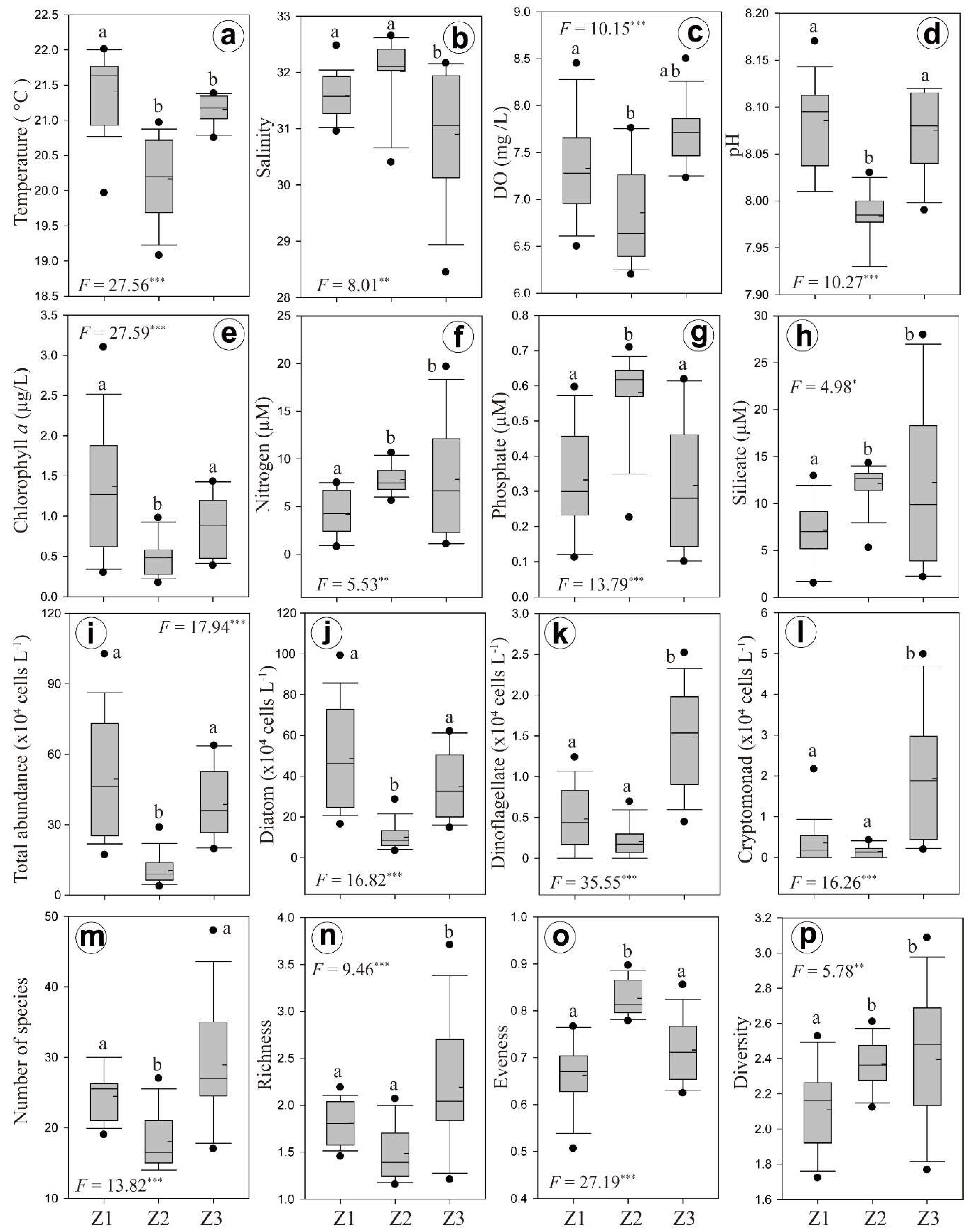
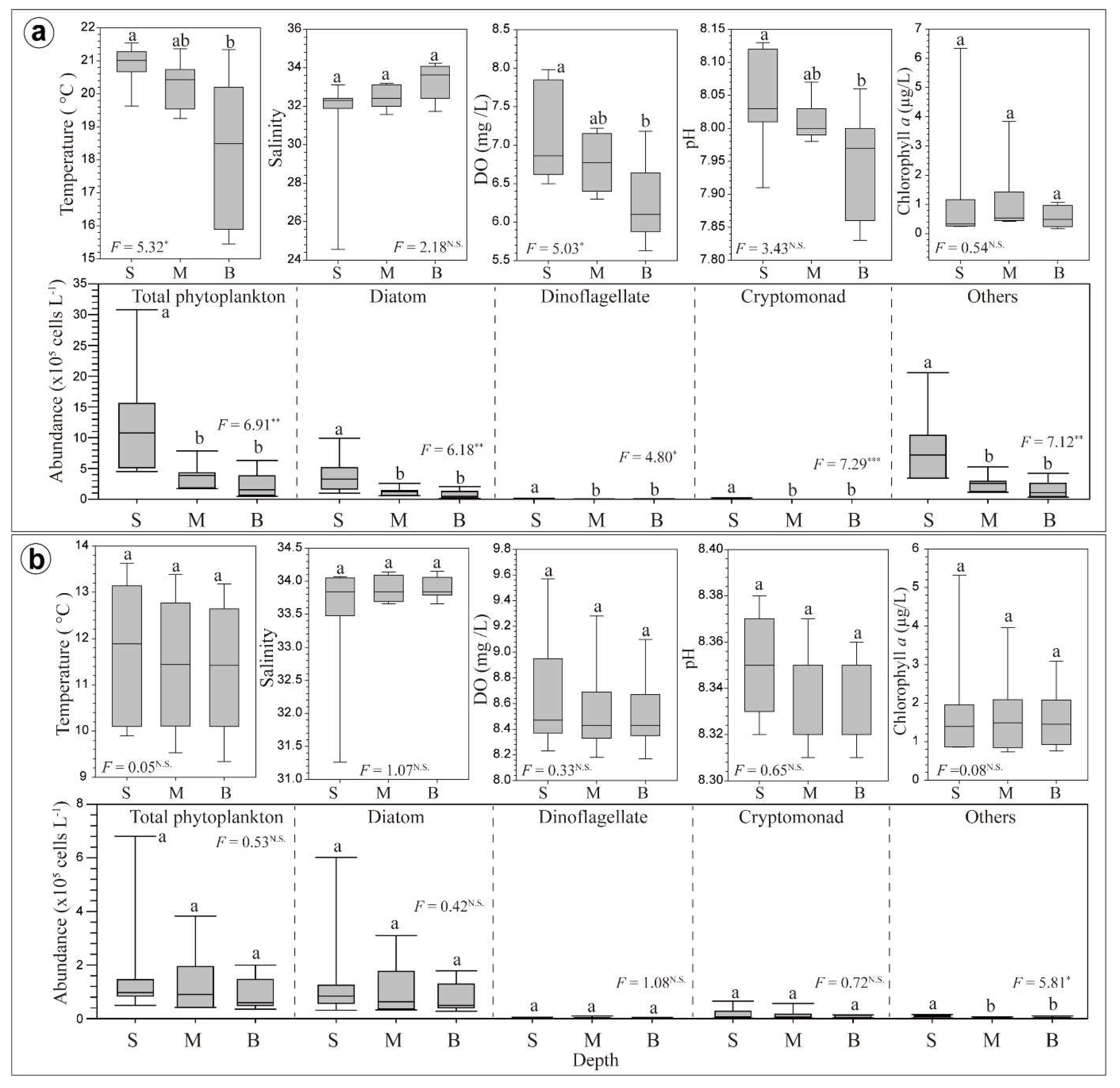
For phytoplankton community analyses, cluster analysis (group average) and non-metric multidimensional scaling (MDS) ordination (based on the Bray-Curtis similarity index) were used for the analysis of species abundance data using SPSS version 17.0 (SPSS Inc., Chicago, IL, USA) [18]. Differences were considered significant when the p value was below 0.05. The differences in abiotic and biotic factors (including phytoplankton abundance) between three geographical zones (see below) were assessed by one-way analysis of variance (ANOVA) with Tukey’s test, and the differences between surface and bottom layers were evaluated by the t-test using SPSS version 17.0. Canonical correspondence analysis (CCA) can explain the relationships between a community and the environment. The impact of the measured environmental factors on the occurrences of dominant phytoplankton at the genus and species levels was investigated by CCA using CANOCO for Windows 4.5 software. The measured environmental factors, including temperature, salinity, ammonia, nitrate + nitrite, phosphate, and silicate, were the explanatory variables. Ln(x+1) transformation was performed on the phytoplankton data for CCA ordination. In addition, principal component analysis (PCA) was performed for season-averaged abiotic and biotic factors to identify environmental factors that were related to phytoplankton dynamics. Statistical computations for these procedures were performed using XLSTAT 2010 (AddionSoft ^TM).

3. Results

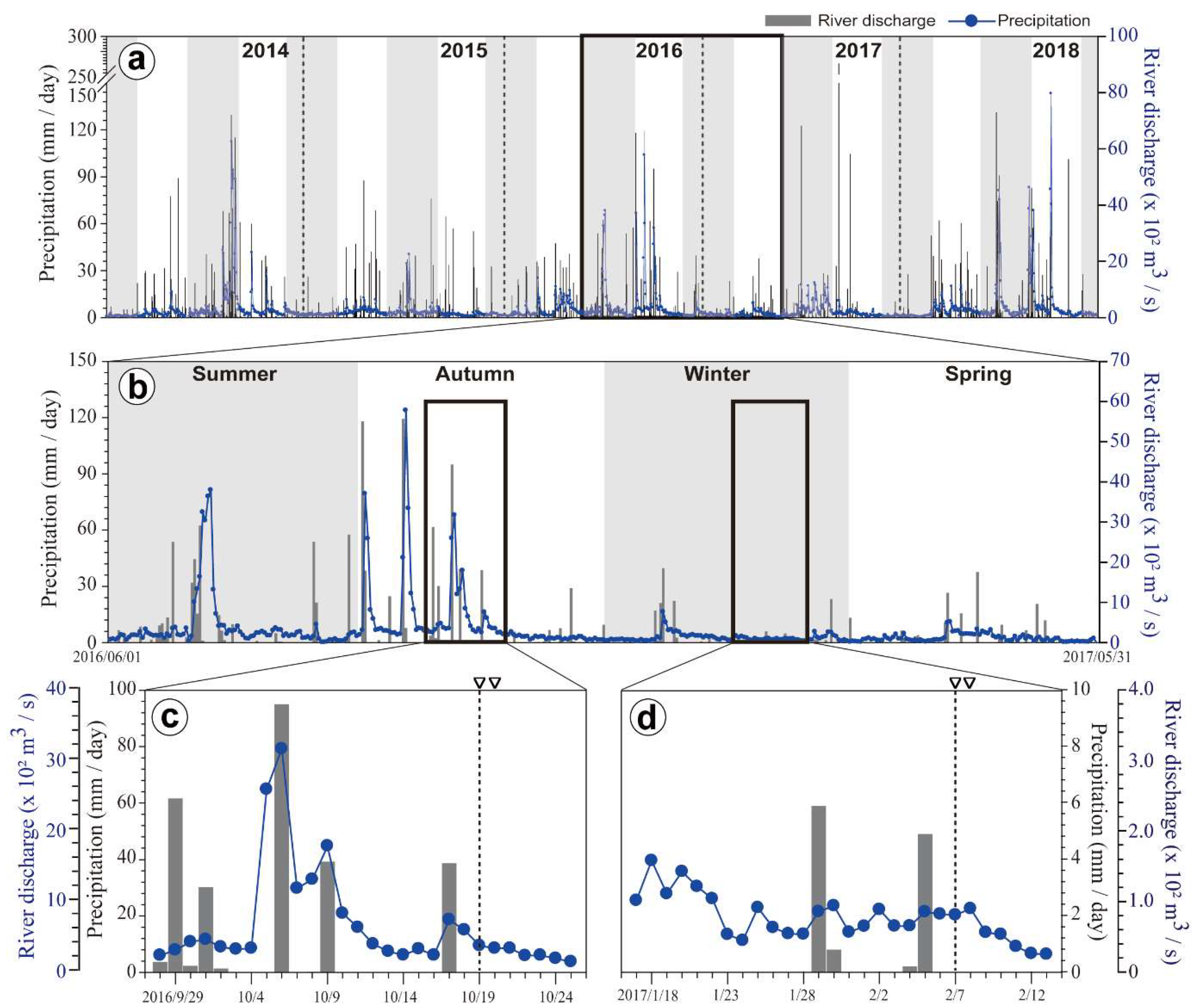
3.1. Precipitation and River Discharge

Figure 2 shows the daily precipitation and river discharge data for the Nakdong River from 2014 to 2018. The amounts of both were generally high during summers and low during winters. From summer 2016 to spring 2017, the daily river discharge and precipitation were significantly increased during autumn and remained low until the spring of the next year. In particular, there was a large amount of rainfall and river discharge after the passage of Typhoon Chaba on 5 October (Figure 2b). The two-week accumulated river discharge and precipitation prior to the sample date were greater during autumn (October) than the other three seasons, and these remained low during winter (February).

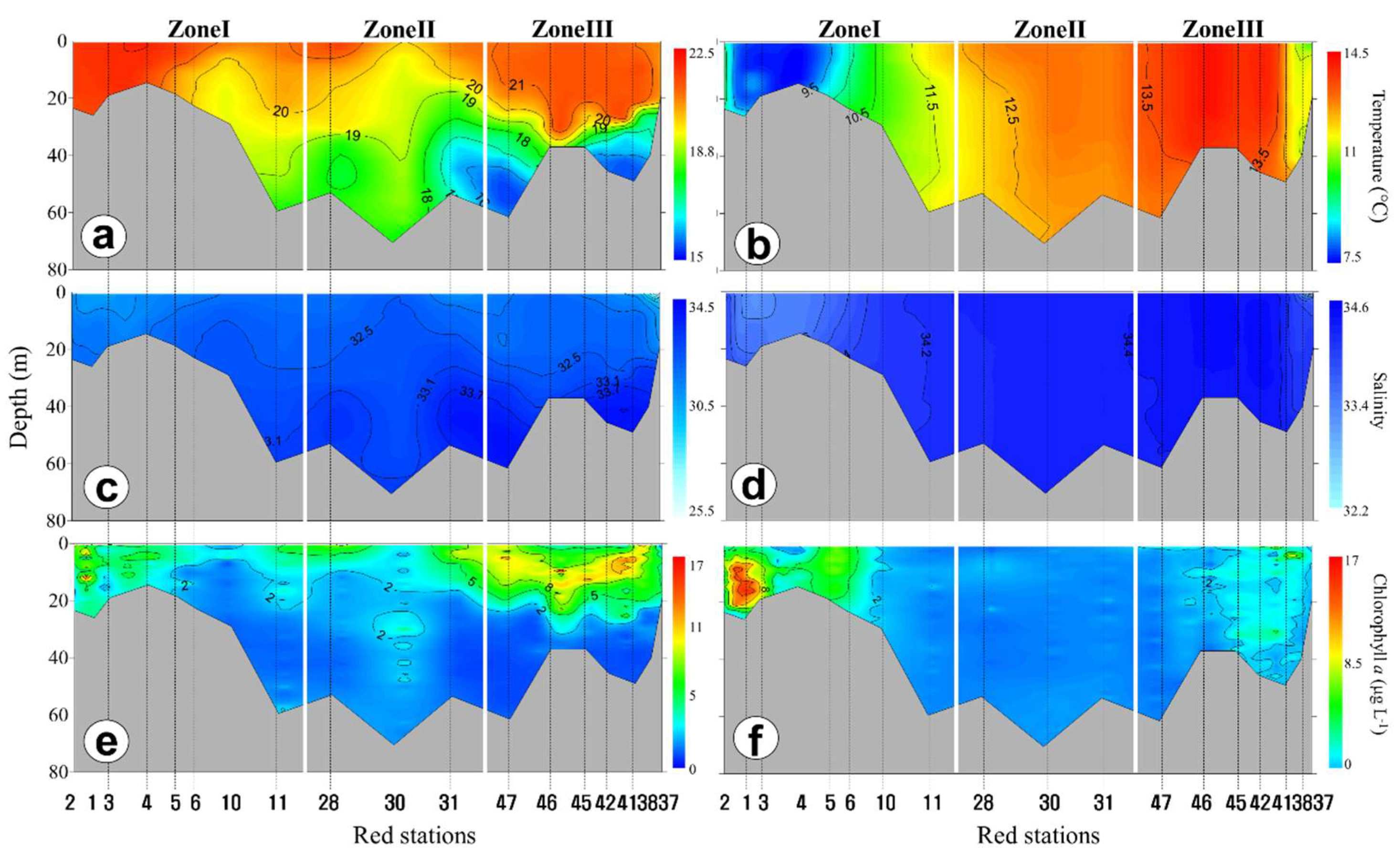
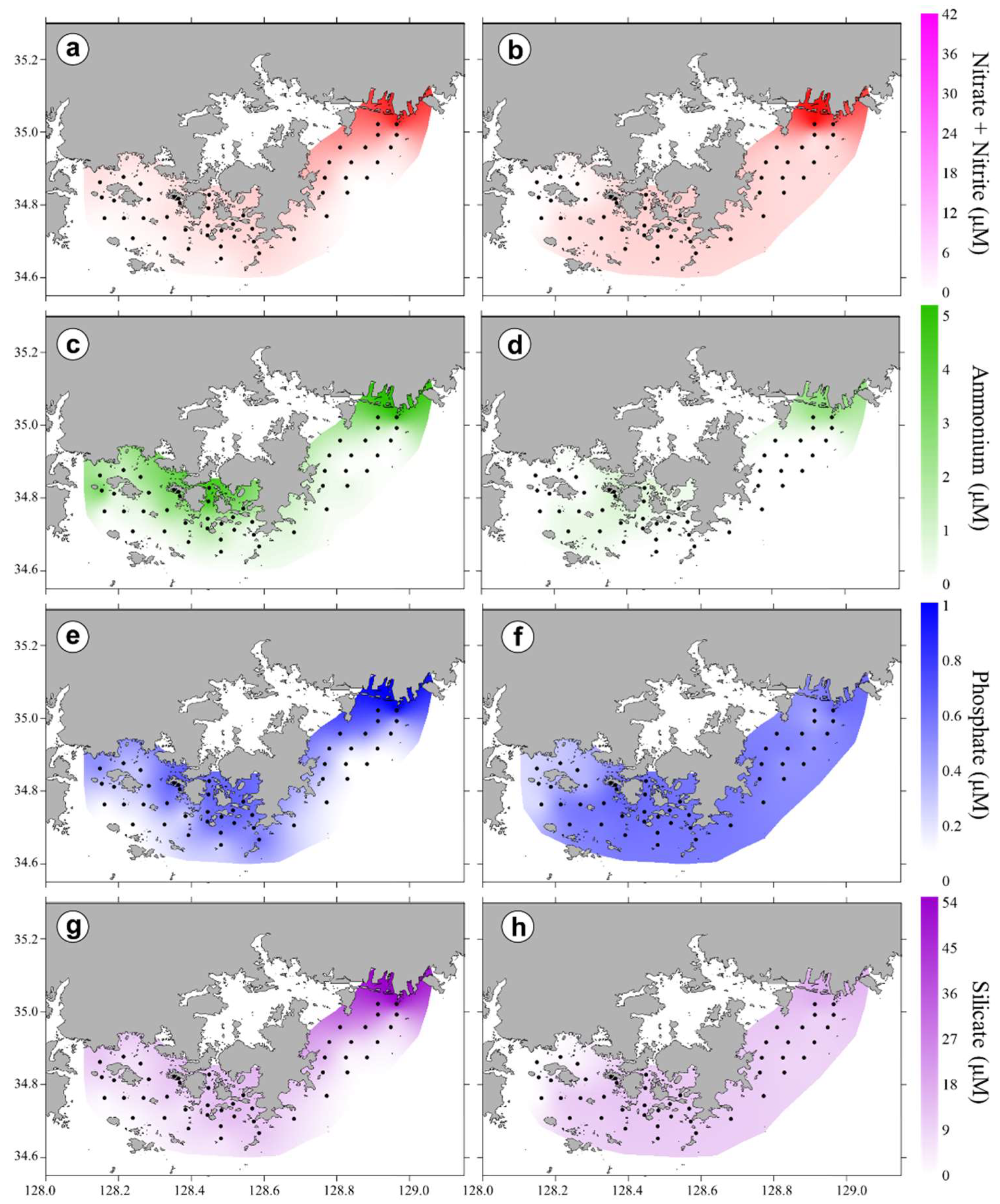
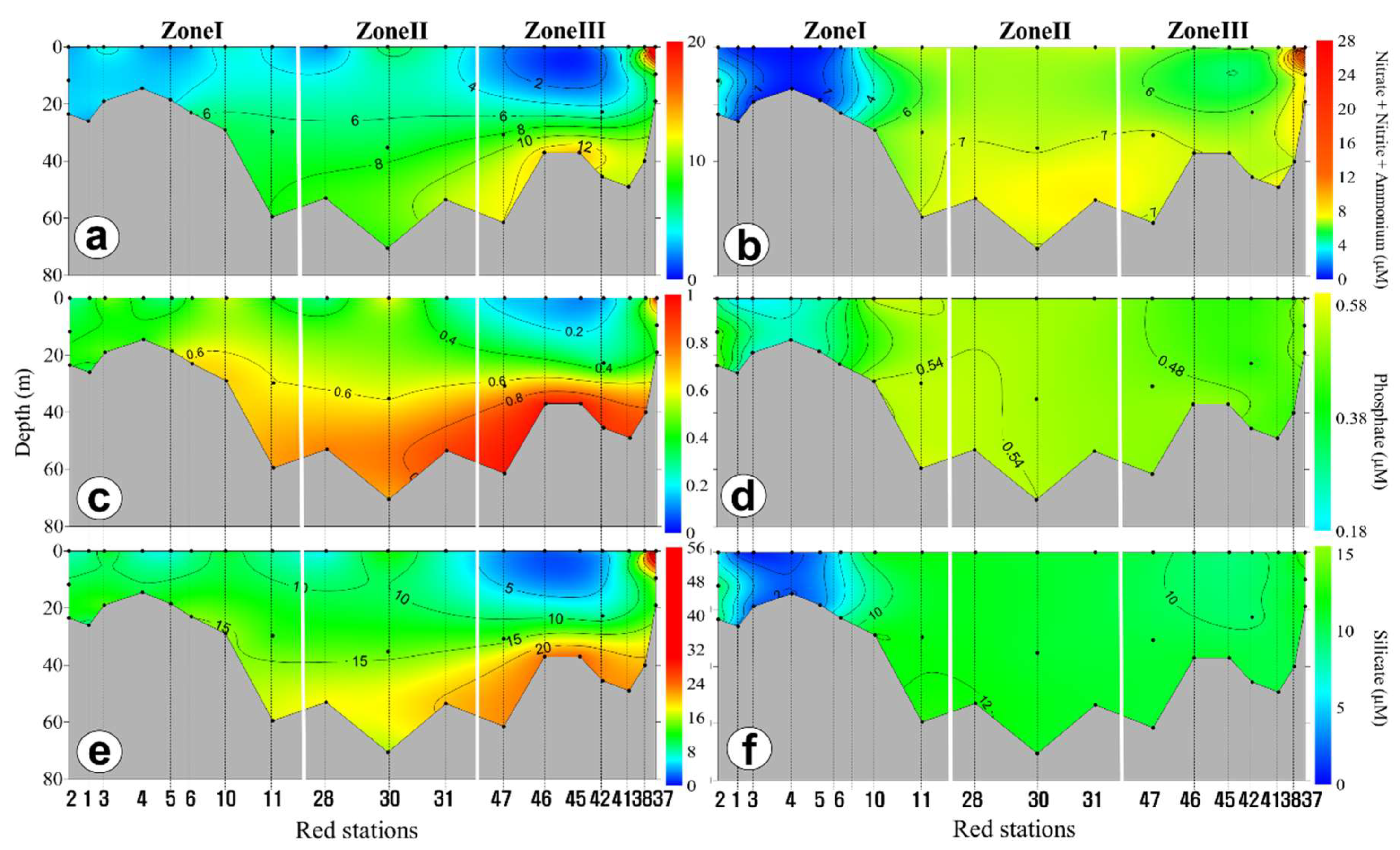
3.2. Horizontal and Vertical Distributions of Environmental Factors

The horizontal surface seawater temperature (SST) at the 47 stations varied during October, from 19.2 °C (Zone II) to 22.0 °C (Zone I) (Figure 3a). The average SST of Zone II was more than two degrees lower than that of the other zones. In contrast, the SST also varied greatly during February, ranging from 7.7 °C (inshore of Zone I) to 14.1 °C (Zone III) (Figure 3b). The water temperature at the outer coastal region (Stations 12, 13, 14, 15, and 16) in Zone I were relatively high (~14°C), and formed a strong temperature front between the outer and inner coastal regions in Zone I (Figure 3b). Salinity in the surface layer decreased dramatically after rainfall during October, and the lowest salinity was 26.8; however, salinity during February also exhibited a small spatial variation in the surface layer, varying from 30.4 to 32.7, excluding Station 37 of the Nakdong Estuaries (Figure 3c). The pH did not vary greatly during October and February. The pH during October gradually increased from 7.8 to 8.0 from the inner to the outer coastal regions (Figure 2e,f). In contrast, pH during February was relatively low in the outer coastal region of Zone I (Figure 3e,f). DO was greater during February than October and ranged from 6.3 to 8.3 mg L⁻¹ during October and 8.2 to 10.3 mg L⁻¹ during February (Figure 3g,h).

Analysis of the vertical profiles indicated that water temperature during October had a strong vertical stratification in Zone III, except at Station 37, and was gradually stratified in Zone II (Figure 4). The water temperature during October ranged from 15.4 to 22.2°C. During February, the water column was well mixed vertically, and the temperature differences among the three zones were greater (Figure 4b). During October, there was high salinity from the bottom to the surface, but the salinity was relatively low in the upper layer (0 to 3 m) at Station 37 of Zone III, near the Nakdong Estuaries (Figure 4c). In contrast to October, high-salinity water (> 32) was common at Zone II and III during February (Figure 3d and Figure 4d).

There were large spatial variations in dissolved inorganic nutrients (Figure 5). During October, the nitrate + nitrite concentration varied from 0.64 to 37.4 µM; it was higher in and around the Nakdong Estuaries of Zone III and lower in the inner regions of Zone I. There were also variations in the concentrations of ammonia (0.04 to 5.1 µM), phosphate (0.1 to 1.0 µM), and silicate (1.5 to 54.3 µM), with higher levels at the inner regions than the outer coastal regions. The ranges of nutrient concentrations during October were similar to those during February, but the horizontal distribution patterns were different, and the concentrations were high at most stations during February. In particular, there were high nutrient levels during both seasons in the mouths of the Nakdong Estuaries, where freshwater was discharged. In the vertical profile of October, the nitrogen concentration was constant vertically but was low at the surface layer of several stations.

Analysis of the vertical distributions of nutrients indicated that phosphate and silicate were higher in the bottom layers (Figure 6). During February, these high nutrient levels in the whole water column were maintained, except at Zone I. Among these nutrients, the nitrogen was high at Station 37 (Nakdong Estuaries) and the nitrogen and silicate concentrations were low at the inner coastal regions of Zone I.

The average Shannon-Weaver (H′) diversity of phytoplankton was 2.29 during October, and the greatest H′ was 2.40 at Zone III. The average evenness (J′) was 0.74, and the greatest J′ was 0.83 at Zone II. During February, the average H′ was 2.30 and the average J′ was 0.78, and both of these parameters were greatest at Zone II.

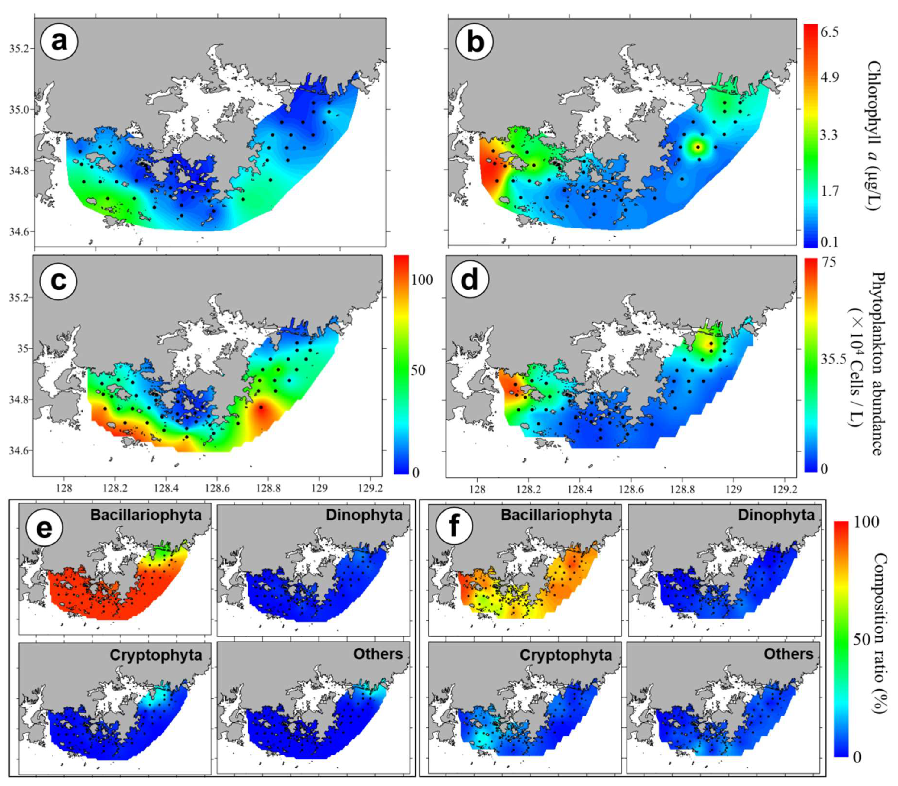
3.3. Chl-a Concentration and Presence of Different Phytoplankton

Figure 7 shows the spatial and temporal variations of Chl-a concentration and phytoplankton abundance. The surface Chl-a concentration varied from 0.3 to 3.1 µg L^–1 during October and from 0.6 to 6.13 µg L^–1 during February. The Chl-a concentration was about 2-fold higher during February than October. In particular, the Chl-a concentration in October was high in outer coastal water but was high at the inner coastal regions during February. The total phytoplankton abundance varied from 3.7 × 10⁴ to 8.4 × 10⁵ cells L^–1 (mean ± SD: 3.3 × 10⁵ cells L^–1 ± 2.4 × 10⁵) in October (Figure 6c) and from 3.8 × 10⁴ to 7.1 × 10⁵ cells L^–1 (mean ± SD: 2.1 × 10⁵ cells L^–1 ± 2.0 × 10⁵) during February (Figure 5c). During October and February, diatoms accounted for more of the total phytoplankton biomass at all of the stations, and the levels of dinoflagellates and cryptophytes were relatively low. The distribution of cryptophytes differed during October and February.

We analyzed the abundances of the dominant phytoplankton genera, which were composed of eight diatoms and one cryptophyte (Figure 8). During October, the diatom Chaetoceros spp. was dominant at Zones I and II, and Pseudo-nitzschia spp. had a high abundance at Zone II. The second most dominant groups were the diatoms Eucampia spp., Skeletonema spp., Pseudo-nitzschia spp., and Asterionella glacialis. During February, E. zodiacus was present at the inshore area of Zone I, and Skeletonema spp. and Chaetoceros spp. had relatively high levels at Zone III. Overall, the freshwater diatom Stephanodiscus spp. had a high abundance at Station 37 (Nakdong Estuaries of Zone III). The abundance of cryptophytes was relatively high at Zone III during October and at Zone I during February.

We performed cluster analysis and non-metric MDS to assess the phytoplankton composition and to quantify phytoplankton during each month (Figure 9 and Figure 1c). The results indicated that the phytoplankton community structure separated into three distinct groups during October and February (p < 0.001). During October, the phytoplankton community structure at Zone II was the most distinct in that it had a 50% similarity to the other clusters. All of the stations at Zone I were located at the inner and outer coastal regions of Tongyeong, and most stations that branched at Zone II were in the semi-closed area of the western parts of Geoje Island. All stations at Zone III were in the inner and outer coastal waters of the Nakdong Estuaries. During February, Zone I (located at the inner coastal water of Tongyeong) had a 61% similarity to the other clusters. Most stations at Zone II were in the outer coastal regions of the southern area of Geoje Island, which branched at 58%. In addition, Zone III (located at the inshore and offshore regions of Nakdong Estuaries) branched at 38%. Overall, this analysis indicated that the geographical characteristics of phytoplankton were similar during October and February.

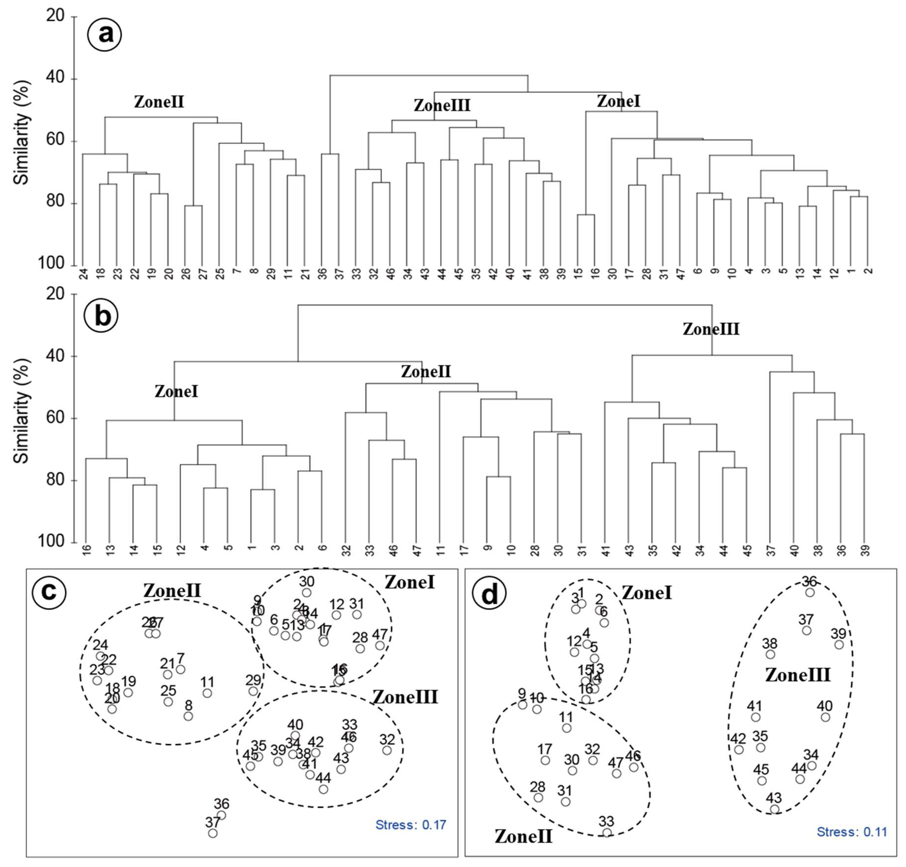
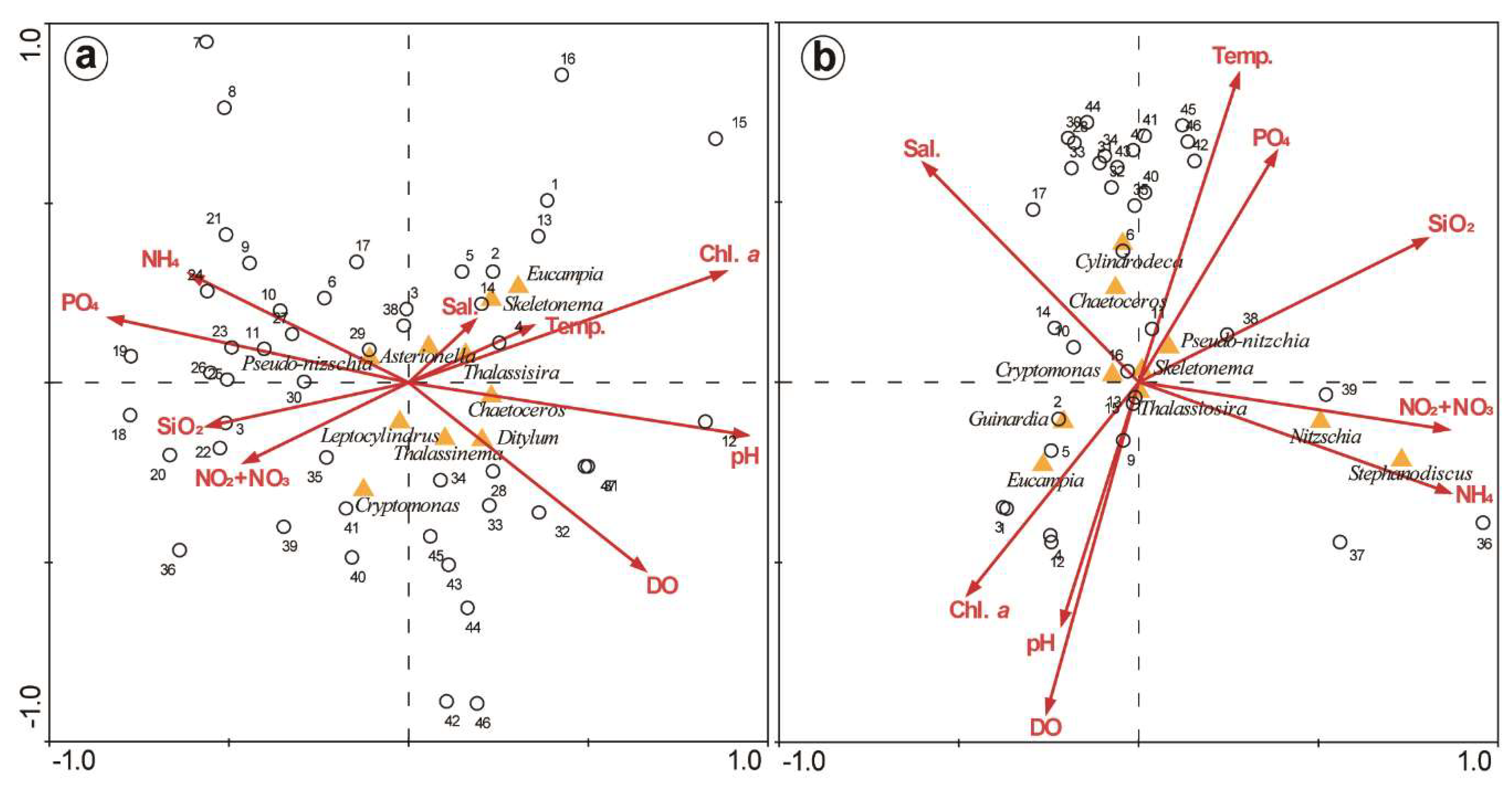
3.4. PCA and CCA of Factors Affecting Phytoplankton

We performed PCA to identify environmental factors that affected phytoplankton dynamics during both sampling periods (

Table 1. Loadings of the first three principal components from principal component analysis (PCA) of the surface waters during October and February. Loadings greater than 0.6 or less than −0.6 are in bold.

	October			February
	PC1	PC2	PC3	PC1	PC2	PC3
Temperature	–0.56	–0.30	–0.50	–0.85	–0.10	0.47
Salinity	–0.32	0.73	0.45	–0.53	–0.80	0.10
NO2 + NO3	0.75	–0.59	–0.16	–0.17	0.96	0.12
NH4	0.70	0.13	–0.47	0.03	0.90	–0.28
PO4	0.94	0.08	–0.11	–0.88	0.24	–0.25
SiO2	0.82	–0.49	–0.17	–0.74	0.61	–0.02
Chl-a	–0.77	–0.17	–0.42	0.86	–0.15	0.21
DO	–0.62	–0.51	0.03	0.93	0.10	–0.14
pH	–0.93	–0.17	–0.02	0.78	0.01	0.40
Total phytoplankton	–0.82	–0.36	–0.23	0.88	0.17	0.28
Total diatom	–0.84	–0.29	–0.25	0.87	0.14	0.28
Total dinoflagellate	–0.14	–0.68	0.48	–0.30	–0.19	0.45
Total cryptophyte	0.18	–0.72	0.33	0.73	–0.07	–0.16
Others	0.56	–0.64	–0.28	0.20	0.78	0.28
Eigenvalue	6.61	3.62	1.87	7.12	3.59	1.53
Variability (%)	44.05	24.15	12.45	47.47	23.96	10.21
Cumulative %	44.05	68.20	80.65	47.47	71.43	81.64

). During October, Principal Component 1(PC1) accounted for 44.5% of the variance, and there were large positive loadings for NO₂ + NO₃, NH₄, silicate, and phosphate and large negative loadings for Chl-a, pH, DO, total phytoplankton, and diatoms. PC2 accounted for 24.1% of the variance, and only had large negative loadings for dinoflagellates, cryptophytes, and other species. During February, PC1 accounted for 47.5% of the variance and there were strong negative loadings for water temperature, phosphate, and silicate, and strong positive loadings for Chl-a, pH, DO, total phytoplankton, diatoms, and cryptophytes. PC2 accounted for 24.0% of the variance, and there was a strong negative loading for salinity, and strong positive loadings for NO₂ + NO₃, NH₄, silicate, and other species.

Our CCA analysis indicated that there was a relationship between environmental factors (water temperature, salinity, pH, DO, and inorganic nutrients) and the dominant phytoplankton groups during October and February (Figure 10). During October, the dominant diatom species had similar abundances, with Chaetoceros, Eucampia, and Skeletonema grouping together. These genera had positive correlations with Chl-a, salinity, and temperature and negative correlations with NO₂ + NO_3, NH₄, phosphate, and silicate. During February, there was a positive relationship of temperature with phosphate and these two factors had negative correlations with pH and DO. The genus Eucampia had a positive correlation with Chl-a, implying that species in this genus were mostly responsible for the high Chl-a levels. In addition, the freshwater diatom Stephanodiscus spp. had a positive correlation with nutrient levels, particularly nitrogen compounds.

4. Discussion

4.1. Relationship of Phytoplankton Bloom With High Nutrient Level After Typhoon Chaba

According to path of Typhoon Chaba, phytoplankton primary production was significantly increased in Korean coastal waters during the autumn. The increased levels of nutrients in coastal waters can have a significant impact on annual primary production [11] and can determine phytoplankton community structure [19,20]. In this study, an increase in precipitation due to Typhoon Chaba during the two weeks led to an elevation of the Nakdong River discharge, resulting in nutrients loading to the nearby coastal waters; there were significant negative relationships between salinity and nutrients at Zone III (NO₂ + NO₃, r = –0.92, p < 0.001; NH₄, r = −0.72, p < 0.001; PO₄, r= −0.95, p < 0.001; and SiO₂, r = −0.94, p < 0.001), implying that the abundant nutrients from the river discharge were supplied to Zone III and remained present even 2 weeks after the typhoon. Based on our data, there was a time lag (two weeks) between nutrient loading and the increase in phytoplankton abundance in this study. Similar to with our data, a time lag (two weeks) between two events has occasionally been observed in Korean coastal waters, even when this introduction is sudden [8].

4.2. Spatial and Temporal Variations of Biotic and Abiotic Factors

There was a clear difference in phytoplankton community structure between Zone III and Zones I and II; diatom species were the common dominant taxa in all three zones, but flagellated species (dinoflagellates and cryptophytes) were predominant only in the estuarine waters (Zone III). Moreover, the species number, diversity, and richness of phytoplankton at Zone III were greater than at Zones I and II (p < 0.01; ANOVA). Interestingly, based on our measurement data, abiotic conditions at Zone III were clearly distinct, compared to the other two zones; the salinity was slightly lower at Zone III than at Zone I and Zone II (F = 8.01, p < 0.01; ANOVA; Figure 11), implying a significant influence by the Nakdong River discharge after the typhoon. In addition, the main nutrients at Zone III (nitrogen and silicate) were significantly greater there than at Zones I and II (nitrogen, F = 5.53, p < 0.01; silicate, F = 4.98, p < 0.05). Smayda [4] demonstrated that water movements and environmental factors in the water column can strongly affect the spatio-temporal distribution of phytoplankton. Therefore, together with these findings, the spatio-temporal difference of abiotic factors among the three zones might lead to variation in the phytoplankton community structure in southern Korean coastal waters.

Our analysis of surface biotic and abiotic factors during the winter indicated that the water temperature of the inshore area at Zone I was significantly lower than at Zones II and III (F = 23.3, p < 0.01; ANOVA; Figure 12). This suggests that a relatively high water temperature was maintained within the Busan coastal water (Zone III) because of the introduction of a large amount of warm water from the TWC and a relatively small input of cold freshwater from the Nakdong River during the winter. Baek et al. [9] reported that the Busan coast is affected by the TWC throughout the year, and thus has relatively warm water (>10°C) even during winter. Whereas, we found no difference in salinity between the three zones (p > 0.01; ANOVA). However, the DO and pH at Zone I were higher than at Zones II and III (DO: F = 15.51, p < 0.01; pH: F = 4.39, p < 0.05; ANOVA), which may be related to the high level of Chl-a at Zone I (Zone I vs. Zone II and Zone III; F = 8.32, p < 0.05; ANOVA). Based on previous findings, the DO concentration and pH level typically correlate with phytoplankton population density (Chl-a) and daytime photosynthesis [21,22]. Therefore, higher phytoplankton biomass at Zone I may lead to an elevation of the DO and pH levels in the winter season.

In contrast, the levels of nitrogen, phosphate, and silicate were significantly lower at Zone I than at Zones II and III (nitrogen: F = 4.57, p < 0.05; phosphate: F = 11.93, p < 0.01; silicate: F = 13.17, p < 0.01; ANOVA), implying a greater uptake of these nutrients by phytoplankton (especially diatoms) at Zone I. This result indicates that the high abundance of diatoms at Zone I was largely responsible for the high total phytoplankton abundance. Moreover, although the number of dinoflagellates did not differ among the zones (p > 0.01; ANOVA), the total abundance of phytoplankton, diatoms, and cryptophytes was greater at Zone I than at Zones II and III (p < 0.01; ANOVA). In addition, the phytoplankton diversity and evenness were lower at Zone I than at Zones II and III, implying that the phytoplankton diversity may have declined because of the dominance of the diatom E. zodiacus during the winter. E. zodiacus, a large centric diatom species, has a worldwide distribution and sometimes forms dense blooms during winter and early spring in Korean coastal waters [2], suggesting that this species can grow in cold water, as noted below.

4.3. Vertical Variations of Biotic and Abiotic Factors

We analyzed the biotic and abiotic factors in the whole water column to examine the impact of vertical water mixing by the typhoon during the autumn and of wind-mediated water turbulence during the winter. During the autumn, the temperature, DO, and pH at the surface were significantly greater than at the middle and bottom layers (p < 0.001; ANOVA; Figure 13). Although salinity at the surface layer had significant variations between areas, it did not differ significantly between the surface, middle, and bottom layers (F = 2.18, p > 0.01; ANOVA). The Chl-a level also did not differ between the three layers (p > 0.01; ANOVA), although the total phytoplankton (F = 6.91), diatoms (F = 6.18), dinoflagellates (F = 4.80), and cryptophytes (F = 7.29) were more abundant in the surface layer than the middle and bottom layers (p < 0.01; ANOVA). Whereas, biotic and abiotic factors during the winter did not differ between the three layers (p > 0.01; ANOVA), implying that both water mixing by windstorm events and the low temperature of the surface layer promoted mixing of the whole water column (Figure 13b). We found that phytoplankton responded to the nutrient increase that occurred following wind-driven mixing of the water column, and there is evidence that blooms in other regions also occurred following continuous winter water mixing due to wind events in temperate coastal waters [23]. It is well known that wind affects water stability and turbulence. Our finding of high phytoplankton abundance during the winter throughout the whole water column is similar to the findings of Yin et al. [23] and Baek et al. [9]. These results thus confirm that mixing of the whole water column by winter windstorms and low surface temperature (due to the sinking of high-density water) is likely to be a key event in regulating the biotic and abiotic characteristics of the water column. In particular, a water mixing event during winter has an important role in driving diatom species from the surface layer to the middle and bottom layers. [2,24,25].

4.4. Phytoplankton Community Structure and Characteristics of Phytoplankton Species

It is well known that spatial and temporal variability of environmental parameters can affect phytoplankton community structure in coastal waters. During October, our cluster analysis and MDS analysis separated the phytoplankton community into three major groups (p < 0.001). Most stations had high densities of the centric diatom Chaetoceros spp. (including C. didymus and C. lorenzianus), and this is known as a cosmopolitan species. In particular, diatom species accounted for 92.7% of the total phytoplankton species, and four diatoms (Chaetoceros spp., Skeletonema spp., E. zodiacus, and Pseudo-nitzschia spp.) accounted for approximately 84.6% of the total. The second most dominant species were Skeletonema spp. and E. zodiacus at Zone I, Pseudo-nitzschia spp. at Zone II, and small Cryptomonas spp. at Zone III. Based on our CCA, the abundances of Chaetoceros, Eucampia, and Skeletonema had positive correlations with Chl-a, implying that they were responsible for the high phytoplankton biomass during the autumn. Baek et al. [2] reported that a large introduction of nutrients following heavy precipitation in the inner area of Gwangyang Bay (Korea) led to a large bloom of diatoms (especially Skeletonema spp.) during summer. Tsuchiya et al. [19,20] demonstrated that 5 days after the passage of a summer typhoon at Sagami Bay (Japan), the dominant dinoflagellates shifted to diatom groups, such as Chaetoceros spp. and Cerataulina spp. Thus, this shows high nutrient input following typhoon-stimulated diatom blooms, as in the present study. In contrast, we found that Cryptomonas spp. (primarily flagellates) occurred in regions with a relatively low salinity and high levels of nutrients at Zone III. Our previous seasonal survey also demonstrated that Cryptomonas spp. were predominant (> 70%) during the autumn in the Seomjin estuarine region in Gwangyang Bay [2] and in the Nakdong Estuary [9]. As demonstrated by Klaveness [26], cryptophytes grow well in the presence of pulsed nutrient loading and tend to dominate when nutrient conditions are non-limiting. Therefore, the nutrient loading after a typhoon increases the abundances of diatom species, especially Chaetoceros spp.; in contrast, Cryptomonas spp. were opportunists that appeared when the diatom biomass was relatively low, particularly at Zone III sites.

In February, the zone classified as Zone I was dominated by Eucampia, and Zone II consisted of low diatom populations. The communities affected by the river were classified as Zone III. The stations adjacent to the estuary of the Nakdong River were high in Chaetoceros and Nitzschia (first dominated groups) along the Nakdong Estuary, as well as Stephanodiscus and Thalassiosira (second dominated groups). In particular, the diatom E. zodiacus was the predominant species at the inner coastal regions of Zone I. Based on our CCA results, the abundance of E. zodiacus had a positive correlation with Chl-a, pH, and DO and a negative correlation with water temperature; this implies that this species contributed to the total phytoplankton biomass when the water temperature was low. E. zodiacus has a worldwide distribution, and sometimes forms dense populations during the relatively low temperatures of winter and early spring [2,27]. Nishikawa et al. [28] reported that E. zodiacus was present throughout the year in temperate coastal waters and was most abundant from February to April, in agreement with our results. Additionally, based on current findings, a high biomass of phytoplankton (mostly E. zodiacus) at Zone I in winter is thought to lead to an increase in pH level and DO concentration, resulting in a positive correlation between this diatom and these two chemical factors. Moreover, Stephanodiscus hantzschii, a harmful freshwater diatom, mainly appeared when salinity was low and nutrient levels were high. In particular, the abundance of S. hantzschii had a positive correlation with nitrogen nutrients and a negative correlation with salinity, thus explaining their higher abundance when there is a continuous overflow of freshwater. Baek et al. [9] reported that a high density of the S. hantzschii was present in Nakdong estuarine water, and this is known as a winter-blooming species in Korea [29]. In addition, this harmful freshwater diatom can tolerate low levels of salinity and can even survive in the saltwater conditions of the Nakdong Estuary. This explains the maintenance of abundant S. hantzschii in estuarine waters.

In conclusion, multiple environmental variables present in a coastal area have complex effects on the phytoplankton community. We analyzed these environmental variables in Korean coastal waters to better understand the ecological dynamics of phytoplankton following Typhoon Chaba (October 2016) and a winter water mixing event (February 2017), with a focus on physical, chemical, and biological variables. The changes in the phytoplankton community structure had clear correlations with some of the same environmental factors in all three coastal zones, although there were slight differences between autumn and winter. Nutrient dynamics fluctuated due to Typhoon Chaba. The resulting inflow of fresh water from the estuary area and the large amount of freshwater from the Nakdong River had large effects on the phytoplankton community in the southern sea of Korea during the autumn of 2016. Moreover, the introduction of abundant nutrients into the euphotic layers during a winter mixing period coincided with a high biomass and reproduction of diatoms and the vertical dispersal of these cells. Our results thus indicate that internal and external environmental factors triggered changes in the phytoplankton community during Typhoon Chaba and the subsequent winter turbulence event in Korean coastal waters.

References

1. Thompson, P.A.; Bonham, P.I.; Swadling, K.M. Phytoplankton blooms in the Huon Estuary, Tasmania: Top-down or bottom-up control? J. Plankton Res. 2008, 7, 735–753. [Google Scholar] [CrossRef] [Green Version]
2. Baek, S.H.; Kim, D.S.; Son, M.H.; Yun, S.M.; Kim, Y.O. Seasonal distribution of phytoplankton assemblages and nutrient enriched bioassays as indicators of nutrient limitation of phytoplankton growth in Gwangyang Bay, Korea. Estuar. Coast. Shelf Sci. 2015, 163, 265–278. [Google Scholar] [CrossRef]
3. Eppley, R.W.; Rogers, J.N.; McCarthy, J.J. Half-saturation constants for uptake of nitrate and ammonium by phytoplankton. Limnol. Oceanogr. 1969, 14, 912–920. [Google Scholar] [CrossRef]
4. Smayda, T.J. Harmful algal blooms: Their ecophysiology and general relevance to phytoplankton blooms in the sea. Limnol. Oceanogr. 1997, 42, 1137–1153. [Google Scholar] [CrossRef]
5. Baek, S.H.; Shimode, S.; Han, M.S.; Kikuchi, T. Growth of dinoflagellates Ceratium furca and Ceratium fusus in Sagami Bay, Japan: The role of nutrient. Harmful Algae 2008, 7, 729–739. [Google Scholar] [CrossRef]
6. Anderson, D.M.; Glibert, P.M.; Burkholder, J.M. Harmful algal blooms and eutrophication: Nutrient sources, composition, and consequences. Estuaries 2002, 25, 704–726. [Google Scholar] [CrossRef]
7. Thomas, W.H.; Gibson, C.H. Effects of small-scale turbulence on microalgae. J. Appl. Phycol. 1990, 2, 71–779. [Google Scholar] [CrossRef]
8. Baek, S.H.; Shimode, S.; Kim, H.C.; Han, M.S.; Kikuchi, T. Strong bottom-up effects on phytoplankton community caused by a rainfall during spring and summer in Sagami Bay, Japan. J. Mar. Syst. 2009, 75, 253–264. [Google Scholar] [CrossRef]
9. Baek, S.H.; Kim, D.; Kim, Y.O.; Son, M.; Kim, Y.J.; Lee, M.; Park, B.S. Seasonal changes in abiotic environmental conditions in the Busan coastal region (South Korea) due to the Nakdong River in 2013 and effect of these changes on phytoplankton communities. Cont. Shelf Res. 2019, 175, 116–126. [Google Scholar] [CrossRef]
10. Chen, Y.I.; Chen, H.; Jan, S.; Tuo, S. Phytoplankton productivity enhancement and assemblage change in the upstream Kuroshio after typhoon. Mar. Ecol. Progr. Ser. 2009, 385, 111–126. [Google Scholar] [CrossRef]
11. Tsuchiya, K.; Yoshiki, T.; Nakajima, R.; Miyaguchi, H.; Kuwahara, V.S.; Taguchi, S.; Kikuchi, T.; Toda, T. Typhoon-driven variations in primary production and phytoplankton assemblages in Sagami Bay, Japan: A case study of typhoon Mawar (T0511). Plankton Benthos Res. 2013, 8, 74–87. [Google Scholar] [CrossRef] [Green Version]
12. Townsend, D.W.; Keller, M.D.; Sieracki, M.E.; Ackleson, S.G. Spring phytoplankton blooms in the absence of vertical water column stratification. Nature 1992, 360, 59–62. [Google Scholar] [CrossRef]
13. Baek, S.H.; Lee, M.; Kim, Y.B. Spring phytoplankton community response to an episodic windstorm event in oligotrophic waters offshore from the Ulleungdo and Dokdo islands, Korea. J. Sea Res. 2018, 132, 1–14. [Google Scholar] [CrossRef]
14. Isobe, A. On the origin of the Tsushima Warm Current and its seasonality. Cont. Shelf Res. 1999, 19, 117–133. [Google Scholar] [CrossRef]
15. Lie, H.J.; Cho, C.H. On the origin of the Tsushima Warm Current. J. Geophys. Res. Oceans 1994, C12, 25081–25091. [Google Scholar] [CrossRef]
16. Takikawa, T.; Yoon, J.H. Volume transport through the Tsushima Straits estimated from sea level difference. J. Oceanogr. 2005, 61, 699–708. [Google Scholar] [CrossRef] [Green Version]
17. Hwang, C.S.; Kim, K.T.; Oh, C.Y.; Jin, C.G.; Choi, C.U. A study on correlation between RUSLE and estuary in Nakdong River watershed. J. Korean Soc. Geosp. Inform. Syst. 2010, 18, 3–10. [Google Scholar]
18. Field, J.; Clarke, K.; Warwick, R. A practical strategy for analysing multispecies distribution patterns. Mar. Ecol. Prog. Ser. 1982, 8, 37–52. [Google Scholar] [CrossRef]
19. Tsuchiya, K.; Kuwahara, V.S.; Yoshiki, T.; Nakajima, R.; Miyaguchi, H.; Kumekawa, N.; Kikuchi, T.; Toda, T. Phytoplankton community response and succession in relation to typhoon passages in the coastal waters of Japan. J. Plankton Res. 2014, 36, 424–438. [Google Scholar] [CrossRef] [Green Version]
20. Tsuchiya, K.; Kuwahara, V.S.; Tomoko, M.; Yoshiki, T.; Nakajima, R.; Shimode, S.; Kikuchi, T.; Toda, T. Response of phytoplankton and enhanced biogeochemical activity to an episodic typhoon event in the coastal waters of Japan. Estuar. Coast. Shelf Sci. 2017, 194, 30–39. [Google Scholar] [CrossRef]
21. Kunlasak, K.; Chitamanat, C.; Whangchai, N.; Promya, J.; Lebel, L. Relationships of dissolved oxygen with Chlorophyll a and phytoplankton composition in Tilapia Ponds. Int. J. Geosci. 2013, 4, 46–53. [Google Scholar] [CrossRef] [Green Version]
22. Hinga, K.R. Effects of pH on coastal marine phytoplankton. Mar. Ecol. Prog. Ser. 2002, 238, 281–300. [Google Scholar] [CrossRef]
23. Yin, K.; Harrison, P.J.; Goldblatt, R.H.; St. John, M.A.; Beamish, R.J. Factors controlling the timing of the spring bloom in the Strait of Georgia estuary, British Columbia, Canada. Can. J. Fish. Aquat. Sci. 1997, 54, 1985–1995. [Google Scholar] [CrossRef]
24. Mikaelyan, A.S. Winter bloom of the diatom Nitzschia delicatula in the open waters of the Black Sea. Mar. Ecol. Prog. Ser. 1995, 129, 241–251. [Google Scholar] [CrossRef]
25. Kakehi, S.; Ito, S.I.; Kuwata, A.; Saito, H.; Tadokoro, K. Phytoplankton distribution during the winter convective season in Sendai Bay, Japan. Cont. Shelf Res. 2015, 97, 43–53. [Google Scholar] [CrossRef] [Green Version]
26. Klaveness, D. Biology and ecology of the cryptophyceae: Status and challenges. Biolog. Oceanogr. 1989, 6, 257–270. [Google Scholar]
27. Ito, Y.; Katano, T.; Fujii, N.; Koriyama, M.; Yoshino, K.; Hayami, Y. Decreases in turbidity during neap tides initiate late winter blooms of Eucampia zodiacus in a macrotidal embayment. J. Oceanogr. 2013, 69, 467–479. [Google Scholar] [CrossRef]
28. Nishikawa, T.; Hori, Y.; Tanida, K.; Imai, I. Population dynamics of the harmful diatom Eucampia zodiacus Ehrenberg causing bleaching of Porphyra thalli in aquaculture in Harima-Nada, the Seto Inland Sea, Japan. Harmful Algae 2007, 6, 763–773. [Google Scholar] [CrossRef]
29. Jung, S.W.; Kwon, O.Y.; Lee, J.H. Effect of wter temperature and silicate on the winter blooming diatom Stephanodiscus hantzschii (Bacillariophyceae) growing in eutriphic conditions in the lower Han River, South Korea. J. Freshwater Ecol. 2009, 24, 219–226. [Google Scholar] [CrossRef] [Green Version]
Figure 1. (a) Location of the Korean Peninsula and water masses that affect the South Korean coast. (b) Track of Typhoon Chaba, with blue symbols indicating the range affecting the study area. (c) Sampling stations and the zones of each survey. Each survey was divided into three zones based on cluster analysis of the phytoplankton community (see Figure 9). Each zone was displayed in red (Zone I), green (Zone II), and blue (Zone III). The dotted line represents the groups of the October survey and the filled line represents the groups of the February survey. A vertical survey was conducted in the red marked stations (see Figure 4 and Figure 6). TWC, Tsushima Warm Current; TWWC, Taiwan Warm Water Current; CDW, Changjiang-Diluted Water.
Sustainability 12 02781 g001
Figure 2. (a) Precipitation at Busan and the river discharge of the Nakdong River from 2014 to 2018. (b) Precipitation and river discharge from June 2016 to May 2017. (c) Precipitation and river discharge 3 weeks before and 1 week after the October survey. (d) Precipitation and river discharge 3 weeks before and 1 week after the February survey. Dotted lines in c and d indicate sampling dates.
Sustainability 12 02781 g002
Figure 3. Horizontal distributions of temperature during (a) October and (b) February, salinity during (c) October and (d) February, pH during (e) October and (f) February, and dissolved oxygen (DO) during (g) October and (h) February. The contour maps were drawn using the software Surfer Version 12.
Sustainability 12 02781 g003
Figure 4. Vertical profiles of temperature during (a) October and (b) February, salinity during (c) October and (d) February, and chlorophyll-a (Chl-a) during (e) October and (f) February along the red stations shown in Figure 1c. The contour maps were drawn using the software Surfer Version 12.
Sustainability 12 02781 g004
Figure 5. Horizontal distributions of inorganic nutrients; nitrate + nitrite during (a) October and (b) February, ammonium during (c) October and (d) February, phosphate during (e) October and (f) February, and silicate during (g) October and (h) February. The contour maps were drawn using the software Surfer Version 12.
Sustainability 12 02781 g005
Figure 6. Vertical profiles of inorganic nutrients along the red stations shown in Figure 1c. Nitrogen (Nitrate + Nitrite + Ammonium) during (a) October and (b) February, phosphate during (c) October and (d) February, and silicate during (e) October and (f) February. The contour maps were drawn using the software Surfer Version 12.
Sustainability 12 02781 g006
Figure 7. Horizontal distributions of Chl-a during (a) October and (b) February, total phytoplankton abundance during (c) October and (d) February, and specific horizontal phytoplankton classes (diatoms, dinoflagellates, cryptophytes, and others) during (e) October and (f) February. The contour maps were drawn using the software Surfer Version 12.
Sustainability 12 02781 g007
Figure 8. Horizontal distributions of the 1st dominant genus in each station during (a) October and (b) February, and the 2nd dominant genus in each station during (c) October and (d) February. Each zone, separated by multidimensional scaling (MDS), is marked with a colored line; Red: zone I, Yellow: zone II, and Blue: zone III. Cluster analysis of the phytoplankton community. The contour maps were drawn using the software Surfer Version 12.
Sustainability 12 02781 g008
Figure 9. Cluster analysis of phytoplankton assemblages during (a) October and (b) February, and multidimensional scaling (MDS) analysis during (c) October and (d) February (see Figure 1c.).
Sustainability 12 02781 g009
Figure 10. Canonical correspondence analysis of the relationships of the dominant phytoplankton genera and environmental factors (temperature, salinity, Chl-a, DO, pH, and inorganic nutrients (NO2 + NO3, NH4, PO4, and Si)) during (a) October and (b) February.
Sustainability 12 02781 g010
Figure 11. Box plots of environmental and biological factors in the surface waters of the three zones during October. Median: solid line within the box. Results were from one-way ANOVA, “a” and “b” indicate significant differences, N.S.—not significant, *** p < 0.05, ** p < 0.01, and * p < 0.005.
Sustainability 12 02781 g011
Figure 12. Box plots of environmental and biological factors in the surface waters of the three zones during February. Median: solid line within the box. Results were from one-way ANOVA. “a” and “b” indicate significant differences, N.S.—not significant, *** p < 0.05, ** p < 0.01, and * p < 0.005.
Sustainability 12 02781 g012
Figure 13. Box plots of abiotic and biotic factors at the surface, middle, and bottom layers of the red station during (a) October and (b) February. Median: solid line within the box. Results were analyzed using one-way ANOVA, “a” and “b” indicate significant differences, N.S.—not significant, *** p < 0.05, ** p < 0.01, and * p < 0.005.
Sustainability 12 02781 g013