Efficiency Analysis of Water Conservation Measures in Sanitary Infrastructure Systems by Means of a Systemic Approach

Abstract
:1. Introduction
2. Materials and Methods
2.1. The Urban Water Use (UWU) Model
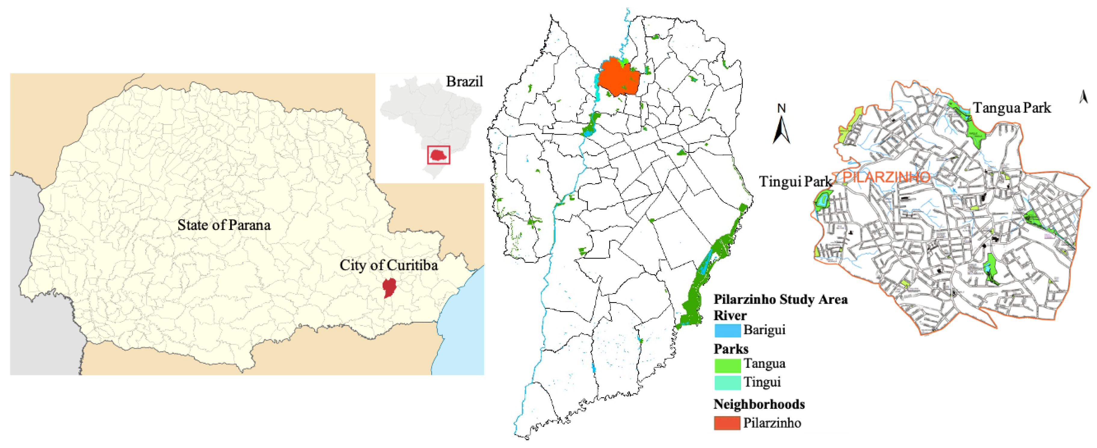
2.2. Case Study
2.3. Study Area
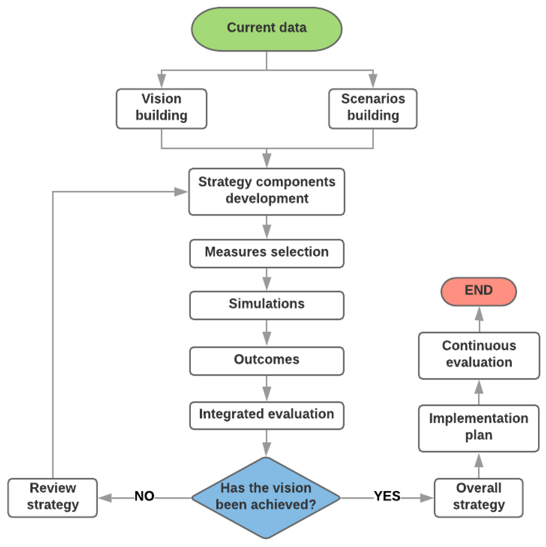
2.4. Vision Building
2.5. Scenario Building
2.6. Measures Group Selection
2.7. Simulation Equations
- is the daily effective per capita consumption (consumed at buildings);
- is the daily total per capita consumption (including water losses at the distribution network);
- is the water loss index at distribution network;
- is the population supplied by WSS;
- is the total population to be served;
- is the highest consumption day coefficient;
- is the populational coverage by WSS.
- is the per capita sewage daily contribution;
- is the population served by SS;
- is the total population to be served;
- is the populational coverage SS.
- is BOD, N, P, and TSS organic loads rates (kg/day);
- is Coliforms organic load rate (day−1);
- is pollutant concentration (mg/L) or (MPN/100 mL);
- is domestic sewage flow (m3/day).
- is runoff coefficient;
- is the maximal rainfall intensity (mm/h);
- is area (ha).
- is annual BOD, N, P and TSS load (kg/year);
- is annual coliform load (year−1);
- is average of annual runoff flow (mm/year);
- is pollutant concentration (mg/l) or (MPN/100 mL);
- is area (m2).
2.8. Outcomes
- is the Effectiveness Index k of the Group of Measures k (GMk);
- is the selected Group of Measures number;
- is the selected indicators number;
- is the number of scenarios in which the indicator i achieved the vision;
- is the indicator i weight.
3. Results and Discussion
4. Conclusions
Author Contributions
Funding
Conflicts of Interest
References
- WEF—World Economic Forum. Global Agenda Council on Risk & Resilience: Resilience Insights; World Economic Forum: Geneva, Switzerland, 2016; 24p. [Google Scholar]
- BRASIL. Lei n° 11,445, de 05 de Janeiro de 2007; Casa Civil: Brasília, Brasil, 2007. [Google Scholar]
- SNIS—Sistema Nacional de Informações sobre Saneamento. Diagnóstico dos Serviços de Água e Esgotos. 2018. Available online: http://www.snis.gov.br/ (accessed on 15 January 2020).
- ABES—Associação Brasileira de Engenharia Sanitária e Ambiental. Situação do Saneamento Básico no Brasil; ABES—Associação Brasileira de Engenharia Sanitária e Ambiental: São Paulo, Brasil, 2015. [Google Scholar]
- ANA—Agência Nacional de Águas. Relatório Conjuntura dos Recursos Hídricos no Brasil: Informe 2017; Agência Nacional de Águas: Brasília, Brasil, 2017. [Google Scholar]
- WE—Water Europe. Water Europe Strategic Innovation and Research Agenda (Water Europe SIRA) 2030; Water Europe: Brussels, Belgium, 2016; ISBN 9789028362161. [Google Scholar]
- Gonzales, P.; Ajami, N.K. Urban water sustainability: An integrative framework for regional water management. Hydrol. Earth Syst. Sci. 2015, 12, 11291–11329. [Google Scholar] [CrossRef] [Green Version]
- Makropoulos, C.K.; Natsis, K.; Liu, S.; Mittas, K.; Butler, D. Decision support for sustainable option selection in integrated urban water management. Environ. Modell. Softw. 2008, 23, 1448–1460. [Google Scholar] [CrossRef]
- Savenije, H.H.G.; Van der Zaag, P. Integrated water resources managagement: Concepts and issues. Phys. Chem. Earth A/B/C 2008, 33, 290–297. [Google Scholar] [CrossRef]
- Bruntland, G.H. Our common Future: The world Commission on Environment and Development; Oxford University Press: Oxford, UK, 1987. [Google Scholar]
- Maurya, S.P.; Singh, P.K.; Ohri, A.; Singh, R. Identification of Indicators for Sustainable Urban Water Development Planning, Ecological Indicators; Elsevier: Amsterdam, The Netherlands, 2020. [Google Scholar]
- Maiolo, M.; Pantuse, D. Sustainable Water Management Index, SWaM Index. Cogent Eng. 2019, 6, 1603817. [Google Scholar] [CrossRef]
- Santos, D.C. Concepção da Infraestrutura Sanitária Urbana Baseada noos Sistemas Prediais Hidráulicos Sanitários (Design of Urban Sanitary Infrastructure Based on Hydraulic Building Systems). XIII Simpósio Nacional de Sistemas Prediais. SISPRED 2019. EPUSP: São Paulo, 2019. Available online: http://sispred13.pcc.usp.br/ (accessed on 9 January 2020).
- Corning, P.A. The Synergism Hypothesis—On the Concept of Synergy and It’s Role in the Evolution of Complex Systems. J. Soc. Evol. Syst. 1998, 21, 133–172. [Google Scholar] [CrossRef]
- Haken, H. Synergetik; Springer: Berlin/Heidelberg, Germany; New York, NY, USA, 1981. [Google Scholar]
- Jaffe, K. The Thermodynamic Roots of Synergy and its Impact on Society; Universidad Simon Bolívar: Caracas, Venezuela, 2017. [Google Scholar]
- Colchester, J. Emergence Theory; System Academy: Barcelona, Spain, 2016. [Google Scholar]
- Tucci, C.E.M.; Goldenfum, J.A.; Parkinson, J.N. Integrated Urban Water Management: Humid Tropics; UNESCO IHP. Urban Water Series; CRC Press: Boca Raton, FL, USA, 2010. [Google Scholar]
- Lawson, E. Learning and Action Alliances to Develop a Blue-Green Vision for Urban Flood Risk Management [online]. EPSRC FCERM.Net Webinar Series. 2015. Available online: http://www.fcerm.net/LearningAlliance (accessed on 27 November 2019).
- Rogers, B.; Hammer, K. Realising the Vision of a Water Sensitive City; The Source: Barrie, ON, Canada, 2019; pp. 24–27. [Google Scholar]
- Vairavamoorthy, K.; Matthews, N.; Brown, P. Building Resilient Urban Water Systems for An Uncertain Future; The Source: Barrie, ON, Canada, 2019; pp. 20–23. [Google Scholar]
- dos Santos, D.C.; van der Steen, P. Understanding the IUWM Principles: An Activity Based on Role Play Approach (for Facilitator and Specialists); UNESCO-IHE: Delft, The Netherlands, 2011; 66p. [Google Scholar]
- dos Santos, D.C.; Benetti, A. Application of the urban water use model for urban water use management purposes. Water Sci. Technol. 2014, 70, 407–413. [Google Scholar] [CrossRef] [PubMed]
- IPPUC—Instituto de Pesquisa e Planejamento Urbano de Curitiba. Nosso Bairro: Pilarzinho; Wons, L., Coord, L.W., Eds.; IPPUC: Curitiba, Brazil, 2015. [Google Scholar]
- SANEPAR—Companhia de Saneamento do Estado do Paraná. Indicadores Operacionais; Companhia de Saneamento do Estado do Paraná: Curitiba, Brazil, 2016. [Google Scholar]
- Giusti, D.A. Contribuição a Geologia Ambiental no Município de Curitiba—PR. Master’s Thesis, Universidade de São Paulo, São Paulo, Brazil, 1989; 115p. [Google Scholar]
- IBGE—Instituto Brasileiro de Geografia e Estatística. Censo Demográfico 2010; Instituto Brasileiro de Geografia e Estatística: Rio de Janeiro, Brazil, 2010; p. 175. [Google Scholar]
- INMET—Instituto Nacional de Meteorologia. BDMEP—Banco de Dados Meteorológicos para Ensino e Pesquisa. 2018. Available online: http://www.inmet.gov.br/projetos/rede/pesquisa/ (accessed on 20 August 2019).
- Agência Curitiba. Perfil Econômico das Regionais. 2018. Available online: http://www.agencia.curitiba.pr.gov.br/perfil-economico-regional (accessed on 14 August 2019).
- Brombach, H.; Weiss, G.; Fuchs, S. A new database on urban runoff pollution: Comparison of separate and combined sewer systems. Water Sci. Technol. 2005, 51, 119–128. [Google Scholar] [CrossRef] [PubMed]
- von Sperling, M.; Chernicharo, C.A.L. Biological Wastewater Treatment in Warm Climate Regions; IWA Publishing: London, UK, 2005; 1460p, ISBN1 1843390027. ISBN2 1843391074. [Google Scholar]
- Bazzarella, B.B. Caracterização e Aproveitamento de Água Cinza para uso não Potável em Edificações. Master’s Thesis, (Mestrado em Engenharia Ambiental)—Programa de Pós-Graduação em Engenharia Ambiental, Universidade Federal do Espírito Santo, Vitória, Brazil, 2005. [Google Scholar]
- ITB—Instituto Trata Brasil. Conselho Empresarial Brasileiro para o Desenvolvimento Sustentável—CEBDS. Benefícios econômicos da expansão do Saneamento. Qualidade de vida Produtividade e Educação Valorização Ambiental; Ex Ante Consultoria Econômica; Instituto Trata Brasi: São Paulo, Brazil, 2014; p. 72. [Google Scholar]
- Maiolo, M.; Mendino, G.; Pantusa, D.; Senatore, A. Optimization of drinking water distribution systems in relation to the effects of climate change. Water 2017, 9, 803. [Google Scholar] [CrossRef]
- Bruggeman, W.; Dammers, E.; van den Born, G.J.; Rijken, B.; van Bemmel, B.; Bouwman, A.; Nabielek, K.; Beersma, J.; van den Hurk, B.; Polman, N.; et al. A. te Linde (2013): Deltascenario’s voor 2050 en 2100 Nadere uitwerking 2012–2013; Deltares: Delft, The Netherlands, 2013; p. 65. [Google Scholar]
- Destro, C.A.M. The Urban Water Use Model as a Tool to Support the Evaluation of Sustainable Drainage Measures in Brazilian Cities. Ph.D. Thesis, Federal University of Parana, Curitiba, Brazil, 2016. [Google Scholar]
- IPCC—Intergovernmental Panel on Climate Change. Climate Change 2014: Synthesis Report. Contribution of Working Groups I, II and III to the Fifth Assessment Report of the Intergovernmental Panel on Climate Change; Pachauri, R.K., Meyer, L.A., Eds.; IPCC: Geneva, Switzerland, 2014; 151p. [Google Scholar]
- Xiong, W.; Li, Y.; Pfister, S.; Zhang, W.; Wang, C.; Wang, P. Improving water ecosystem sustainability of urban water system by management strategies optimization. J. Environ. Manag. 2020, 254, 109766. [Google Scholar] [CrossRef] [PubMed]
- Loucks, D.P. Sustainable water resources managagement. Water Int. 2000, 25, 3–10. [Google Scholar] [CrossRef]
- Rak, J.R.; Tchórzewska-Cieślak, B.; Pietrucha-Urbanik, K. A Hazard Assessment Method for Waterworks Systems Operating in Self-Government Units. Int. J. Environ. Res. Public Health 2019, 16, 767. [Google Scholar] [CrossRef] [PubMed] [Green Version]


| Categories | Input Data | Values | Source |
|---|---|---|---|
| External factors building process | Current population | 12,232 inhabitants | [27] |
| Current population growth rate | 0.76% | [27] | |
| Minimum population growth rate | 0.38% | [27] | |
| Maximum population growth rate | 1.79% | [27] | |
| Type of population growth | Logarithmic | Statistical analysis | |
| Current year | 2018 | - | |
| Future year | 2048 | - | |
| Historic average temperature per year | 17.23 °C | [28] | |
| Historic minimum average temperature per year | 13.14 °C | [28] | |
| Historic maximal average temperature per year | 23.43 °C | [28] | |
| Historic average rainfall | 1474.68 mm/year | [28] | |
| Current average income rate | R$ 3776.22 | [29] | |
| Current minimum income rate | R$ 1653.45 | [29] | |
| Current maximal income rate | R$ 9821.57 | [29] | |
| Return period | 2, 5, and 10 years | - | |
| Time of rainfall | 32 min | Calculated | |
| Water Supply System (WSS) | Current WSS coverage | 100% | [25] |
| Current water per capita consumption | 130.40 l/inhabitants.day | ||
| Water supply network loss index | 37% | ||
| Sewage System (SS) | Current SS coverage | 69.70% | [25] |
| Return coefficient | Calculated | Calculated | |
| Drainage System (DS) | Covered area | 3.05 km2 | [24] |
| Urban basin length | 2 km | [24] | |
| Number of households | 4.917 houses | [27] | |
| Soil permeability coefficient | 10−5 m/s | [26] | |
| Runoff water | |||
| Biological Oxygen Demand | 13 mg/L | [30] | |
| Total Nitrogen | 2.4 mg/L | ||
| Total Phosphorous | 0.42 mg/L | ||
| Total Suspended Solids | 141 mg/L | ||
| Total Coliforms | 5000 MPN/100 mL | ||
| Appliances | Consumed Specific Flowrate | Use Frequency | Use Duration (s) | Persons (inhabitants) | Total of Water Consumption (l/day) |
|---|---|---|---|---|---|
| Toilet (valve) | 6 | 5 | -- | 1 | 30 |
| Toilet (shower) | 0.1 | 1 | 360 | 1 | 36 |
| Toilet (hand basin) | 0.1 | 5 | 12 | 1 | 6 |
| Kitchen (tap) | 0.2 | 3 | 240 | 4 | 36 |
| Garden (tap) | 0.2 | 1 | 180 | 4 | 9 |
| TOTAL (qe) | 130.40 |
| Appliances | BOD (mg/L) | N (mg/L) | P (mg/L) | TSS (mg/L) | Coliforms MPN/100 mL | Source |
|---|---|---|---|---|---|---|
| Toilet (valve) | 400 | 60 | 15 | 450 | 1.00 × 10¹⁰ | [31] |
| Toilet (shower) | 165 | 3.89 | 0.2 | 103 | 3.95 × 10⁴ | [32] |
| Toilet (hand basin) | 265 | 6.2 | 0.6 | 146 | 1.35 × 10² | [32] |
| Kitchen (tap) | 633 | 14.44 | 9.1 | 336 | 1.47 × 10³ | [32] |
| Washing machine | 184 | 4.17 | 14.4 | 53 | 5.37 | [32] |
| Garden (tap) | 0 | 0 | 0 | 0 | 0 | - |
| Systems | Indicators | Weight (W) |
|---|---|---|
| Water Supply System | Water Supply System Coverage (%) - | 10% |
| Sewage System | Sewage System Coverage (%) - | 10% |
| BOD (kg/day) - | 7% | |
| Total Nitrogen (kg/day) - | 7% | |
| Total Phosphorus (kg/day) - | 7% | |
| Total Suspended Solids (kg/day) - | 7% | |
| Total Coliforms (day−1) - | 7% | |
| Drainage System | Maximal Runoff Flow (m3/s) - | 10% |
| BOD (kg/day) - | 7% | |
| Total Nitrogen (kg/day) - | 7% | |
| Total Phosphorus (kg/day) - | 7% | |
| Total Suspended Solids (kg/day) - | 7% | |
| Total Coliforms (day−1) - | 7% |
| External Factors | Scenarios | ||||
|---|---|---|---|---|---|
| Current | SC1 | SC2 | SC3 | SC4 | |
| Population growth (λ) | λ0 | λ1 | λ2 | λ1 | λ2 |
| Annual average temperature (T) | T0 | T1 | T2 | T1 | T2 |
| Economic performance (EP) | EP0 | EP1 | EP1 | EP2 | EP2 |
| Maximal rainfall (imáx) | imáx0 | imáx1 | imáx1 | imáx2 | imáx2 |
| Average rainfall (i) | i0 | i1 | i1 | i2 | i2 |
| External Factors | Scenarios | ||||
|---|---|---|---|---|---|
| Current | SC1 | SC2 | SC3 | SC4 | |
| Population growth (λ = %) | λ0 = 0.76 | λ1 = 0.38 | λ2 = 1.79 | λ1 = 0.38 | λ2 = 1.79 |
| Average temperature (T = °C) | T0 = 17.23 | T1 = 14.64 | T2 = 26.03 | T1 = 14.64 | T2 = 26.03 |
| Economic performance | |||||
| (EP = R$/month) (EP = US$/month) | EP0 = 3776.22 EP0 = 906.29 | EP1 = 1653.45 EP1 = 396.82 | EP1 = 1653.45 EP1 = 396.82 | EP2 = 9821.57 EP2 = 2357.18 | EP2 = 9821.57 EP2 = 2357.18 |
| Maximal rainfall (imáx = mm/h) Average rainfall (iaver = mm/year) | imáx0 = 73.46 i0 = 1474.68 | imáx1 = 84.98 i1 = 1548.42 | imáx1 = 84.98 i1 = 1548.42 | imáx2 = 94.88 i2 = 1769.62 | imáx2 = 94.88 i2 = 1769.62 |
| Identification | Measures | Quantity | Additional Information |
|---|---|---|---|
| Group of Measures 0 (GM0) Current values | (M0): Without measures | Without measures | It considers that no intervention will be adopted for the study area, it corresponds to a control group of measures and for the establishment of vision value. |
| Group of Measures 1 (GM1) Without Sinergy | (M1): Rational Use of Water (M2): Use of Rainwater (M3): Network Loss Ratio Reduction (M4): Use of Grey Waters (M5): Distribution Tanks (M6): Permeable Pavement | Reduce 20% of water use Use 30% of rainwater Reduce 50% of the losses Use 10% of grey water A tank of 2 m3/house 50% of the area using | In GM1 all the measures are calculated separately, that is, without synergy. |
| Group of Measures 2 (GM2) With Sinergy | (M1): Rational Use of Water (M2): Rainwater Use (M3): Network Loss Ratio Reduction (M4): Use of Grey Waters (M5): Distribution Tanks (M6): Permeable Pavement | Reduce 20% of water use Use 30% of rainwater Reduce 50% of the losses Use 10% of grey water A tank of 2 m3/house 50% of the area using | All the previous measures from Group of Measures 1, but calculated together interconnected, with synergy. |
| Group of Measures | External Factors | Scenarios |
|---|---|---|
| SCi (i = 1, 2, 3, 4) | ||
| GMk (k = 0, 1, 2) | Water Supply System Coverage (%) - | |
| Sewage System Coverage (%) - | ||
| BOD (kg/day) - | ||
| Total Nitrogen (kg/day) - | ||
| Total Phosphorus (kg/day) - | ||
| Total Suspended Solids (kg/day) - | ||
| Total Coliforms (day−1) - | ||
| Maximal Runoff Flow (m3/s) - | ||
| BOD (kg/day) - | ||
| Total Nitrogen (kg/day) - | ||
| Total Phosphorus (kg/day) - | ||
| Total Suspended Solids (kg/day) - | ||
| Total Coliforms (day−1) - |
| Categories | Variation Range |
|---|---|
| Excellent | 3.20–4.00 |
| Good | 2.40–3.20 |
| Reasonable | 1.60–2.40 |
| Insufficient | 0.80–1.60 |
| Poor | 0.00–0.80 |
| Groups of Measures | Indicators | Scenarios | Vision | |||
|---|---|---|---|---|---|---|
| SC1 | SC2 | SC3 | SC4 | |||
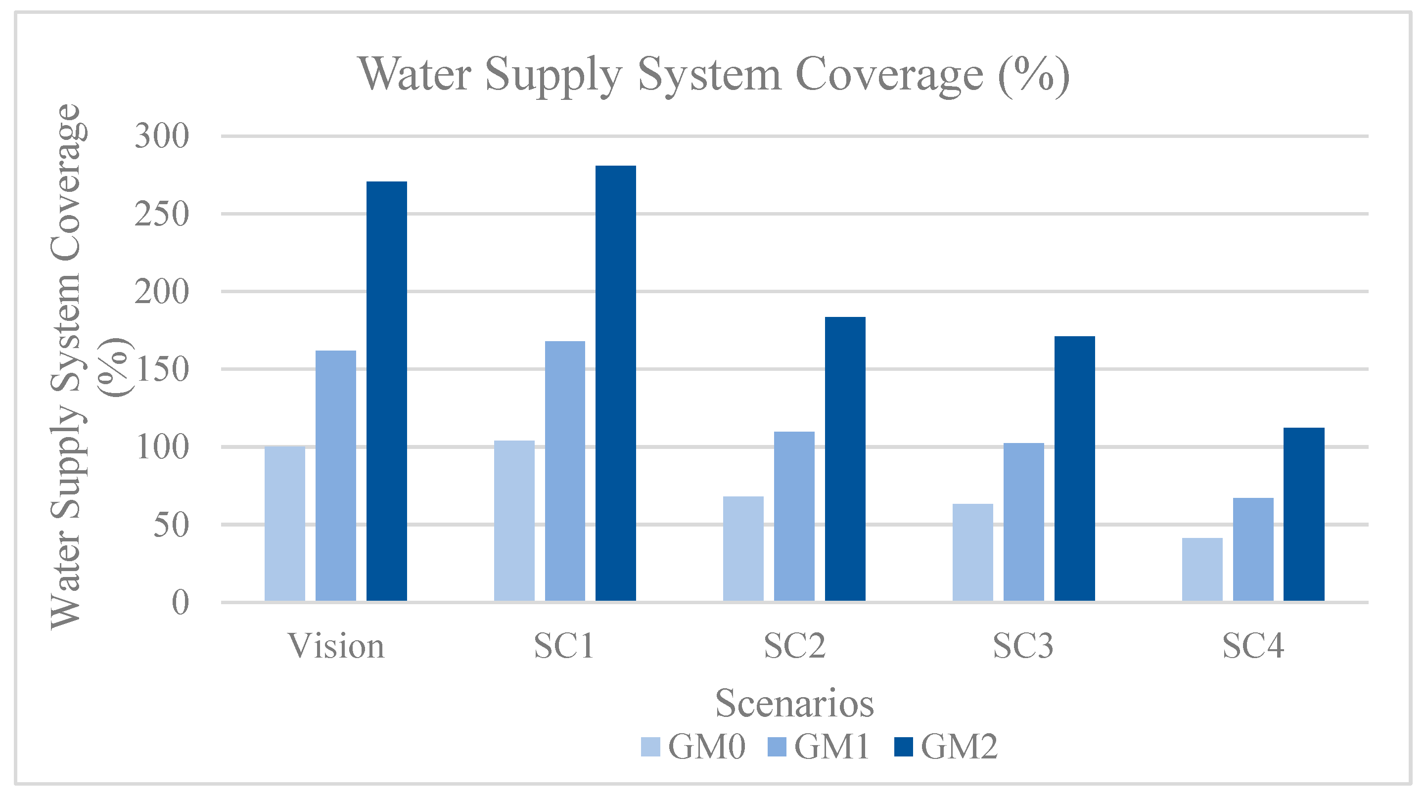
| GM0 Current Values | WSS Coverage (%) | 103.73 | 67.77 | 63.23 | 41.42 | 100.00 |
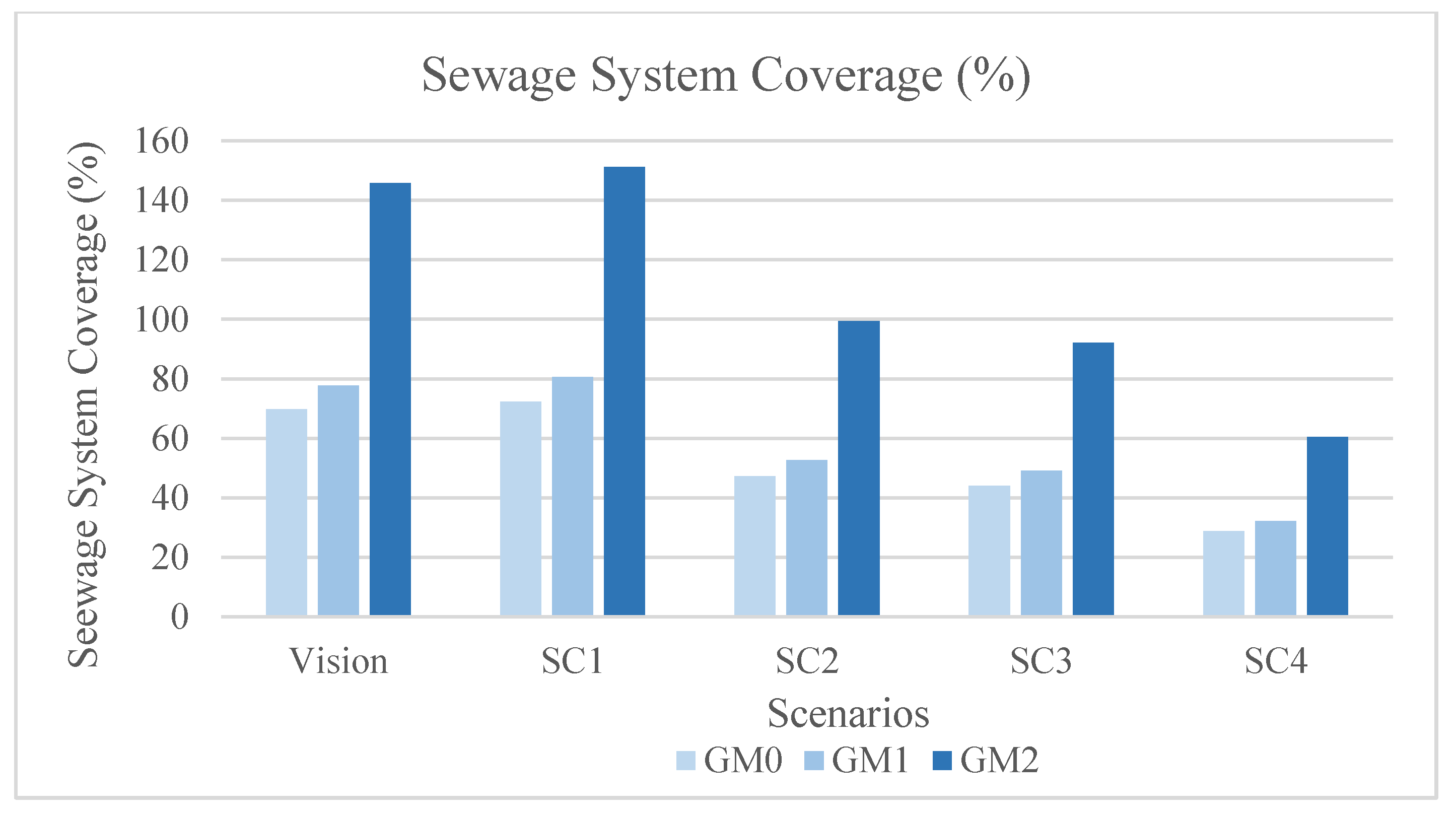
| SS Coverage (%) | 72.30 | 47.24 | 44.07 | 28.87 | 100.00 | |
| BOD (kg/dia) | 471.11 | 474.37 | 772.84 | 776.10 | 548.03 | |
| Total of N (kg/day) | 86.79 | 87.39 | 142.37 | 142.97 | 100.96 | |
| Total of P (kg/day) | 14.15 | 14.25 | 23.22 | 23.31 | 16.46 | |
| Total of SS (kg/day) | 372.20 | 374.78 | 610.58 | 613.16 | 432.96 | |
| Total of Col. (day−1) | 6.05 × 10¹⁹ | 6.13 × 10¹⁹ | 1.63 × 10²⁰ | 1.63 × 10²⁰ | 8.18 × 10¹⁹ | |
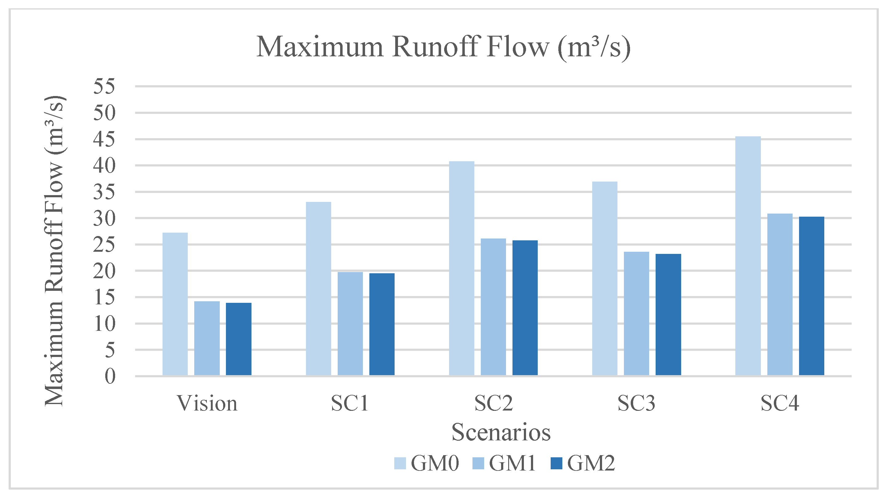
| Max Runoff Flow (m3/s) | 33.06 | 40.74 | 36.92 | 45.49 | 27.21 | |
| BOD (kg/dia) | 77.25 | 95.18 | 88.28 | 108.78 | 70.04 | |
| Total of N (kg/day) | 14.26 | 17.57 | 16.30 | 20.08 | 12.93 | |
| Total of P (kg/day) | 2.50 | 3.08 | 2.85 | 3.51 | 2.26 | |
| Total of SS (kg/day) | 837.82 | 1032.33 | 957.50 | 1179.81 | 759.69 | |
| Total of Col. (day−1) | 2.97 × 10¹² | 3.66 × 10¹² | 3.40 × 10¹² | 4.18 × 10¹² | 2.69 × 10¹² | |
| Groups of Measures | Indicators | Scenarios | Vision | |||
| SC1 | SC2 | SC3 | SC4 | |||
| GM1 Without Sinergy | WSS Coverage (%) | 167.74 | 109.59 | 102.25 | 66.99 | 100.00 |
| SS Coverage (%) | 80.64 | 52.69 | 49.16 | 32.20 | 100.00 | |
| BOD (kg/dia) | 472.53 | 475.80 | 775.17 | 778.44 | 548.03 | |
| Total of N (kg/day) | 87.38 | 87.98 | 143.34 | 143.95 | 100.96 | |
| Total of P (kg/day) | 14.17 | 14.26 | 23.24 | 23.34 | 16.46 | |
| Total of SS (kg/day) | 372.48 | 375.06 | 611.04 | 613.62 | 432.96 | |
| Total of Col. (day−1) | 6.05 × 10¹⁹ | 6.13 × 10¹⁹ | 1.63 × 10²⁰ | 1.64 × 10²⁰ | 8.18 × 10¹⁹ | |
| Max Runoff Flow (m3/s) | 19.75 | 26.08 | 23.61 | 30.82 | 27.21 | |
| BOD (kg/dia) | 42.49 | 52.35 | 48.55 | 59.83 | 70.04 | |
| Total of N (kg/day) | 5.70 | 7.03 | 6.52 | 8.03 | 12.93 | |
| Total of P (kg/day) | 0.87 | 1.08 | 1.00 | 1.23 | 2.26 | |
| Total of SS (kg/day) | 0.00 | 0.00 | 0.00 | 0.00 | 759.69 | |
| Total of Col. (day−1) | 2.97 × 10¹² | 3.66 × 10¹² | 3.40 × 10¹² | 4.18 × 10¹² | 2.69 × 10¹² | |
| Groups of Measures | Indicators | Scenarios | Vision | |||
| SC1 | SC2 | SC3 | SC4 | |||
| GM2 With Sinergy | WSS Coverage (%) | 280.64 | 183.36 | 171.07 | 112.07 | 100.00 |
| SS Coverage (%) | 151.20 | 99.34 | 92.17 | 60.38 | 100.00 | |
| BOD (kg/dia) | 381.39 | 384.03 | 625.65 | 628.29 | 548.03 | |
| Total of N (kg/day) | 70.54 | 71.03 | 115.72 | 116.20 | 100.96 | |
| Total of P (kg/day) | 11.44 | 11.52 | 18.76 | 13.81 | 16.46 | |
| Total of SS (kg/day) | 333.70 | 336.01 | 547.42 | 549.74 | 432.96 | |
| Total of Col. (day−1) | 3.87 × 10¹⁹ | 3.92 × 10¹⁹ | 1.04 × 10²⁰ | 1.05 × 10²⁰ | 8.18 × 10¹⁹ | |
| Max Runoff Flow (m3/s) | 19.51 | 25.77 | 23.16 | 30.27 | 27.21 | |
| BOD (kg/dia) | 39.86 | 48.33 | 44.24 | 53.25 | 70.04 | |
| Total of N (kg/day) | 5.35 | 6.49 | 5.94 | 7.15 | 12.93 | |
| Total of P (kg/day) | 0.82 | 0.99 | 0.91 | 1.09 | 2.26 | |
| Total of SS (kg/day) | 0.00 | 0.00 | 0.00 | 0.00 | 759.69 | |
| Total of Col. (day−1) | 2.79 × 10¹² | 3.38 × 10¹² | 3.09 × 10¹² | 3.72 × 10¹² | 2.69 × 10¹² | |
| Group of Measures | Indicators | Outcomes | Effectiveness Index Σ(N×W) | ||
|---|---|---|---|---|---|
| Number of Scenarios which Achieved the Goal (N) | Vision Weight (W) | N×W | |||
| GM0 Current values | Water Supply System Coverage (%) | 1 | 0.10 | 0.10 | 0.80 Poor |
| Sewage System Coverage (%) | 0 | 0.10 | 0.00 | ||
| BOD (kg/day) | 2 | 0.07 | 0.14 | ||
| Total Nitrogen (kg/day) | 2 | 0.07 | 0.14 | ||
| Total Phosphorus (kg/day) | 2 | 0.07 | 0.14 | ||
| Total Suspended Solids (kg/day) | 2 | 0.07 | 0.14 | ||
| Total Coliforms (day−1) | 2 | 0.07 | 0.14 | ||
| Runoff Flow (l/s) | 0 | 0.10 | 0.00 | ||
| BOD (kg/day) | 0 | 0.07 | 0.00 | ||
| Total Nitrogen (kg/day) | 0 | 0.07 | 0.00 | ||
| Total Phosphorus (kg/day) | 0 | 0.07 | 0.00 | ||
| Total Suspended Solids (kg/day) | 0 | 0.07 | 0.00 | ||
| Total Coliforms (day−1) | 0 | 0.07 | 0.00 | ||
| GM1 Without Synergy | Water Supply System Coverage (%) | 3 | 0.10 | 0.30 | 2.35 Reasonable |
| Sewage System Coverage (%) | 0 | 0.10 | 0.00 | ||
| BOD (kg/day) | 2 | 0.07 | 0.14 | ||
| Total Nitrogen (kg/day) | 2 | 0.07 | 0.14 | ||
| Total Phosphorus (kg/day) | 2 | 0.07 | 0.14 | ||
| Total Suspended Solids (kg/day) | 2 | 0.07 | 0.14 | ||
| Total Coliforms (day−1) | 2 | 0.07 | 0.14 | ||
| Runoff Flow (l/s) | 3 | 0.10 | 0.30 | ||
| BOD (kg/day) | 3 | 0.07 | 0.21 | ||
| Total Nitrogen (kg/day) | 4 | 0.07 | 0.28 | ||
| Total Phosphorus (kg/day) | 4 | 0.07 | 0.28 | ||
| Total Suspended Solids (kg/day) | 4 | 0.07 | 0.28 | ||
| Total Coliforms (day−1) | 0 | 0.07 | 0.00 | ||
| GM2 With Synergy | Water Supply System Coverage (%) | 4 | 0.10 | 0.40 | 2.69 Good |
| Sewage System Coverage (%) | 1 | 0.10 | 0.10 | ||
| BOD (kg/day) | 2 | 0.07 | 0.14 | ||
| Total Nitrogen (kg/day) | 2 | 0.07 | 0.14 | ||
| Total Phosphorus (kg/day) | 3 | 0.07 | 0.21 | ||
| Total Suspended Solids (kg/day) | 2 | 0.07 | 0.14 | ||
| Total Coliforms (day−1) | 2 | 0.07 | 0.14 | ||
| Runoff Flow (l/s) | 3 | 0.10 | 0.30 | ||
| BOD (kg/day) | 3 | 0.07 | 0.21 | ||
| Total Nitrogen (kg/day) | 4 | 0.07 | 0.28 | ||
| Total Phosphorus (kg/day) | 4 | 0.07 | 0.28 | ||
| Total Suspended Solids (kg/day) | 4 | 0.07 | 0.28 | ||
| Total Coliforms (day−1) | 1 | 0.07 | 0.07 | ||
© 2020 by the authors. Licensee MDPI, Basel, Switzerland. This article is an open access article distributed under the terms and conditions of the Creative Commons Attribution (CC BY) license (http://creativecommons.org/licenses/by/4.0/).
Share and Cite
Richter, K.; Santos, D.C.d.; Schmid, A.L. Efficiency Analysis of Water Conservation Measures in Sanitary Infrastructure Systems by Means of a Systemic Approach. Sustainability 2020, 12, 3055. https://0-doi-org.brum.beds.ac.uk/10.3390/su12073055
Richter K, Santos DCd, Schmid AL. Efficiency Analysis of Water Conservation Measures in Sanitary Infrastructure Systems by Means of a Systemic Approach. Sustainability. 2020; 12(7):3055. https://0-doi-org.brum.beds.ac.uk/10.3390/su12073055
Chicago/Turabian StyleRichter, Karoline, Daniel Costa dos Santos, and Aloísio Leoni Schmid. 2020. "Efficiency Analysis of Water Conservation Measures in Sanitary Infrastructure Systems by Means of a Systemic Approach" Sustainability 12, no. 7: 3055. https://0-doi-org.brum.beds.ac.uk/10.3390/su12073055