Multi-Depot Green Vehicle Routing Problem to Minimize Carbon Emissions

Abstract

A Multi-Depot Green Vehicle Routing Problem (MDGVRP) is considered in this paper. In MDGVRP, Alternative Fuel-powered Vehicles (AFVs) start from different depots, serve customers, and, at the end, return to the original depots. The limited fuel tank capacity of AFVs forces them to visit Alternative Fuel Stations (AFS) for refueling. The objective is to minimize the total carbon emissions. A Two-stage Ant Colony System (TSACS) is proposed to find a feasible and acceptable solution for this NP-hard (Non-deterministic polynomial-time) optimization problem. The distinct characteristic of the proposed TSACS is the use of two distinct types of ants for two different purposes. The first type of ant is used to assign customers to depots, while the second type of ant is used to find the routes. The solution for the MDGVRP is useful and beneficial for companies that employ AFVs to deal with the various inconveniences brought by the limited number of AFSs. The numerical experiments confirm the effectiveness of the proposed algorithms in this research.

1. Introduction

According to the report of International Energy Agency (IEA), 23% of global ${\mathrm{CO}}_2$ emissions are generated by the transportation sector, in which nearly 75% of the emissions is generated by the road sector. These figures indicate an emergent need for reducing the ${\mathrm{CO}}_2$ emissions produced by the road sector. Green Logistics emphasizes the sustainable issues arising in logistics operations to diminish the pollution in the road transportation sector. Green logistics advocate the adoption of clean energies, such as electric and hydrogen, to decrease the pollution. The problem regarding the design of the routing scheme for green vehicles is called Green Vehicle Routing Problem (GVRP).

The Green Vehicle Routing problem (GVRP) has attracted attention from researchers due to worldwide environmental concerns [1,2,3]. The classical Vehicle Routing Problem (VRP) focuses mainly on minimizing the total transportation costs of distribution services, while the GVRP addresses sustainable issues in delivery distribution along with the optimal economic cost of delivery [2]. According to [1], the design of GVRP uses Alternative Fuel-powered Vehicles (AFV), which rely on a greener fuel source, such as electricity, natural gas, hydrogen, etc. In addition, Erdoĝan and Miller-Hooks [1] pointed out two main challenges encountered when replacing conventional vehicles with AFVs, namely the limited fuel tank capacity of AFVs and the limited availability of the Alternative Fuel Stations (AFSs). These obstacles add complexity to the model formulation and algorithm design of GVRP.

The Multi-Depot Vehicle Routing Problem (MDVRP) is another branch of the VRP problem which has attracted considerable attention among researchers and practitioners [4,5,6]. In MDVRP, a fleet of vehicles serves customers from several depots and returns back to the same pre-assigned depot. Research about the MDVRP is useful for the companies that have multiple depots.

In recent years, multinational companies such as UPS, Coca-Cola and GM have started paying attention to environmentally sustainable performances for attracting environmentally conscious customers [7,8]. Their objective in this research is to strike a balance between economic performance and environmental protection. For these companies, neither GVRP nor MDVRP may be able to satisfy their objectives. Therefore, in this paper, a model referred to as the Multi-Depot Green Vehicle Routing Problem (MDGVRP) is proposed. Compared to MDVRP or GVRP, MDGVRP has more constraints and, as a result, is more challenging to formulate and solve.

In recent years, the MDGVRP problem has been considered by some researchers [9,10,11,12]. However, compared with their models, our MDGVRP model considers different constraints and objective functions. In their MDGVRP model, the objective function is to minimize the carbon emission generated by the vehicles and does not consider the tank capacity of vehicles. Our model focuses on minimizing the traveling distance of all AFVs with limited tank capacity. Our model is based on Green-VRP (G-VRP), and their models are based on the Pollution Routing Problem (PRP). The G-VRP and PRP are two sub-categories in GVRP, which are discussed in the literature review section.

This paper is organized as follows. In Section 2, a related literature review is presented. Section 3 introduces the definition and formulation of MDGVRP. Section 4 presents the algorithms designed for solving MDGVRP. Numerical experiments are presented in Section 5 and are followed by the conclusion in Section 6.

2. Literature Review

GVRP has received much attention from researchers and academics in recent years due to the fact that people are becoming more conscious about environmental issues. According to a comprehensive literature survey on the GVRP in [2], there are three categories of GVRP, namely Pollution Routing Problem (PRP), Green-VRP (G-VRP) and VRP in reverse logistics. Although these categories focus on economic costs and environment costs simultaneously, the PRP is focused on minimizing the fuel consumption, and the G-VRP is focused on using AFVs instead of conventional vehicles. Therefore, the objective function of PRP is the minimization of the total GHG (Green house gas), and the objective of G-VRP is the minimization of the total travel distance of all AFVs.

In the G-VRP model, tank capacity is considered to be limited. Therefore, vehicles are required to visit AFSs to refuel when the remaining fuel level is not enough to reach the next node on the route. Erdoĝan and Miller-Hooks [1] were the first to address the AFV-based GVRP model. They proposed a model to optimize the transportation routes to overcome the obstacles caused by the limited fuel tank capacity of the AFVs. Based on their work, Felipe, Ortuño, Righini and Tirado [13] proposed a heuristic approach to solve G-VRP with multiple technologies and partial recharges. Montoya et al. [14] developed a multi-space sampling heuristic for G-VRP, and Koç and Karaoglan [15] solved G-VRP with an exact algorithm based on the branch and bound method. Zhang et al. [16] solved G-VRP by using a two-phase meta-heuristic algorithm, while Andelmin and Bartolini [17] also proposed an exact algorithm to solve G-VRP. Peng et al. [18] proposed a memetic algorithm to solve GVRP. Schneider et al. [2] extended the G-VRP by adding the customer time window constraints to the VRP for electric vehicles. All of these papers propose a different variation of the GVRP model based on the GVRP model of Erdoĝan and Miller-Hooks [4] with aim to minimize the total travel distance. The main feature of the GVRP model of Erdoĝan and Miller-Hooks [1] is to introduce limited fuel tank capacity constrains in the VRP model. Our model is based on the GVRP addressed by Erdoĝan and Miller-Hooks [1].

One of the novel features of our model is to minimize the total carbon emissions. Nocera et al. [19] assess the carbon cost emissions for road transportation through traffic flow. They proposed a TANINO model to calculate the carbon emissions of the highway SE30 of a city Seville (Spain). They took road infrastructure, vehicle type and traffic condition into account while estimating carbon emission. Fu et al. [20] proposed a methodology for estimating annual daily traffic and transport emissions for a national road network. These papers estimated the carbon cost for a real-world traffic flow problem. The carbon cost emissions in these articles assumed a linear relationship of carbon cost with the distances travelled by the vehicles, and, hence, our model assumed similar relationship for carbon cost emissions.

Our model is an extension of the multi-depot vehicle routing problem (MDVRP). The MDVRP was first described in Bennett [21]. It is a generalization of the standard VRP in which the number of depots is considered to be more than one [6]. The research of MDVRP mainly focuses on proposing and developing new methods and algorithms to solve the problem. The work of Montoya-Torres et al. [4] revealed that most researchers tend to solve the MDVRP by heuristics or meta-heuristics. For instance, Vidal et al. [5] solved the MDVRP using a hybrid genetic algorithm. Yu et al. [6] converted the MDVRP into a Single-depot VRP (SVRP) by adding a virtual depot in the first step and then by applying an improved Ant Colony Optimization (ACO) to solve the Single-depot VRP (SVRP). Escobar et al. [22] solved MDVRP by using a hybrid granular tabu search algorithm.

The work of Kaabachi et al. [9], Jabir et al. [10], Li et al. [11] and Wang et al. [12] also focuses on MDGVRP; however, their MDGVRP model is developed from the Pollution Routing Problem (PRP) and does not consider the tank capacity of vehicles. One of the aims of this paper is to propose the MDGVRP model with a limited tank capacity of AFVs. Thus, the contribution of the paper includes the introduction of a new MDGVRP model, formulation of a mathematical model for the proposed MDGVRP model, algorithm design for solving the proposed MDGVRP model. Nagy and Salhi [23] solved MDVRP with pickups and deliveries by dividing customers into borderline and non-borderline customers. Based on the idea of Nagy and Salhi [23], a Partition-Based Algorithm (PBA) is proposed in this paper. We also proposed a Two-stage Ant Colony System (TSACS) to obtain high-quality solutions.

3. Problem Description and Formulation

A standard MDGVRP can be described as finding routes with the least distance from more than one depot to a set of customers. Each customer is associated with a fixed allocated demand to be delivered. Each customer is visited by the vehicle fleet only once, and the demand of the customer is satisfied after each visit. A vehicle starts from a depot, serves customers one-by-one, and, finally, returns back to its originally assigned depot. During the service process, when the remaining cargo of a vehicle is not able to satisfy the demand of the next customer, the vehicle returns back to the depot for reloading. If it is necessary to refuel during the service process, the vehicles visit the AFSs for refueling. Therefore, a particular AFS can be visited more than once. The objective of the problem is to minimize the total carbon emissions of operating all vehicles.

In this section, we introduce some definitions and notations that will be used in the rest of the paper. Let $G=\left(V, E\right)$ be a complete and directed graph, in which $V$ is a set of vertices and $E$ is a set of edges between different vertices. The vertex set $V$ has three subsets: customer set $C=\left\{c_1, c_2, \dots c_N\right\}$ for $N$ number of customers, depot set $D=\left\{c_{N+1}, c_{N+2}, \dots c_{N+M}\right\}$ for $M$ number of depots and AFS set $S=\{c_{N+M+1}, c_{N+M+2}, \dots c_{N+M+NS}$} for $NS$ number of AFSs. Therefore, the number of customers, depots and AFSs are $N$, $M$ and $NS$, respectively. For every AFS, $n_f \left(f=1, 2, \dots NS\right)$ is the number of dummy vertices. In this way, the number of visiting times for every AFS can be recorded by $n_f$. In the research of Bard, Huang, Dror, and Jaillet (1998), there are more details and techniques about the use of dummy vertex. The edge set $E=\left\{\left(c_i, c_j\right): c_i, c_j\in V, i\ne j \right\}$ represents the edges connecting different vertices of $V$, and every element of $E$ is associated with the distance between two vertices $d_{ij}$ and fuel consumption $f_{ij}$. In MDGVRP, we assume that the relationship between the travel distance and the fuel consumption is linear. The fuel consumption rate $r$ is assumed to be a fixed value. Therefore, the fuel consumption in arc $\left(c_i, c_j\right)$ is calculated as $f_{ij}=r· d_{ij}$. All other notations used to formulate MDGVRP are defined as follows:

• $K$ The total number of vehicles
• $r$ Fuel consumption rate (gallons per mile)
• $T$ Tank capacity of vehicle (gallons)
• $Q$ Load capacity of vehicle
• $q_i$ The demand of vertex $i$
• $d_{ij}$ The distance in miles between vertices $i$ and $j$
• $C$ The set of customers
• $D$ The set of depots
• $S$ The set of AFSs
• CCF Carbon emission conversion factor
• $DS$ = $D\cup S$ The set contains all depots and AFSs.
• $CS$ = $C\cup S$ The set contains all customers and AFSs.
• $V=C\cup D\cup S$ The set contains all customers, depots and AFSs vertices

Decision Variables

• $x_{ijk}$ is a binary variable taking value 1 if the vehicle travels directly from vertex $i$ to $j$ by the $k^{th}$ vehicle. Otherwise, $x_{ijk}$ takes value 0.
• $f_i$ The remaining fuel level after visiting vertex $i$
• $l_i$ The remaining cargo level after visiting vertex $i$

The mathematical formulation for MDGVRP can be presented as follows:

$$\min {\displaystyle \sum _{i,j\in V}^{}{\displaystyle \sum _{k\in K}^{}{d}_{ij}{x}_{ijk}}}\times CCF$$

(1)

Subject to

$${\displaystyle \sum _{j\in V}{\displaystyle \sum _{k \in K}{x}_{ijk}} = 1, \forall i \in C}$$

(2)

$${\displaystyle \sum _{i\in V}{\displaystyle \sum _{k \in K}{x}_{ijk}} = 1, \forall j \in C}$$

(3)

$${\displaystyle \sum _{i \in V}{x}_{ihk}} - {\displaystyle \sum _{j \in V}{x}_{hjk}} = 0, \forall h \in V, k\in K$$

(4)

$${\displaystyle \sum _{i\in D}{\displaystyle \sum _{j \in V}{x}_{ijk}} \le 1, \forall k \in K}$$

(5)

$$l_j \le l_i - q_j{\displaystyle \sum _{k\in K}{x}_{ijk} + }Q(1-{\displaystyle \sum _{k\in K}{x}_{ijk}}), \forall i \in CS, j \in CS$$

(6)

$$0 \le l_i \le Q - q_i, \forall i \in V$$

(7)

$$f_j \le f_i -r\times d_{ij}{\displaystyle \sum _{k\in K}{x}_{ijk}}+T(1-{\displaystyle \sum _{k\in K}{x}_{ijk}}), \forall i,j \in C$$

(8)

$$f_j \le T -r\times d_{ij}{\displaystyle \sum _{k\in K}{x}_{ijk}}, \forall i \in DS,j \in C$$

(9)

$$f_i \ge r\times d_{ij}{\displaystyle \sum _{k\in K}{x}_{ijk}}, \forall i,j \in V$$

(10)

$$x_{ijk} \in \{0,1\}, \forall i,j \in V, k\in K$$

(11)

In this formulation, Equation (1) is the objective function, which minimizes the total carbon emissions produced by all the vehicles. Constraints (2) and (3) limit each customer to a single visit by a single vehicle. Constraint (4) ensures that, for each vehicle, the number of outgoing arcs from one vertex is equal to the incoming arcs to this vertex. Constraint (5) means that any vehicle $k$ can only leave a depot once. Constraints (4) and (5) combine together to ensure that the starting and ending depot of a vehicle is the same. Constraints (6) and (7) ensure that the vehicle capacity constraint is preserved. Constraints (8)–(10) guarantee that the vehicle tank capacity constraint $T$ is satisfied and these constraints also eliminate sub-tour. In this formulation, Constraints (8)–(10) distinguish the MDGVRP from MDVRP. These constraints are completely different from the other formulation because of the specific property of MDGVRP. Constraint (8) calculates fuel consumption if a vehicle is travelling between two customers. Constraint (9) calculates fuel consumption from depot or fuel station to customer. Constraint (10) ensures that the remaining fuel is enough to go to its next destination. Finally, Constraint (11) limits $x_{ijk}$ to a binary variable. This mathematic model is verified by A Mathematical Programming Language (AMPL), which is introduced in Section 5.

Estimation of Carbon Emission Conversion Factor (CCF)

The research paper of Nocera et al. [19] and Fu et al. [20] estimated carbon cost for real-world traffic flow problem. Nocera et al. [19] estimated the carbon emission by multiplying the total distance travelled by vehicles with the unitary emissions factor. Similarly, Fu et al. [20] estimated carbon emission by multiplying the kilometers of different vehicles (VKMs) with the conversion factor. These two papers motivated us to calculate the carbon emission by multiplying total distances covered by vehicles with the carbon emission conversion factor (CCF). According to Reichmuth et al. [24], a hydrogen-fueled vehicle produces 0.2 kg CO₂ per mile of vehicle travel distance. Thus, we assumed CCF to be 0.20 kg per miles.

4. Solution of MDGVRP

In this section, two methods are designed to solve MDGVRP: the Partition-Based Algorithm (PBA) and the Two-stage Ant Colony System (TSACS) algorithm. The details of these algorithms are provided in the following sections.

4.1. Partition-Based Algorithm (PBA)

The Partition-Based Algorithm (PBA), which is based on the idea of dividing customers into borderline and non-borderline customers, was proposed by Nagy and Salhi (2005) [23] to solve MDVRP. In this paper, we extend the PBA for solving MDGVRP. A borderline customer is a customer who is situated approximately halfway between two depots. For instance, consider customer $i$ with the nearest depot $p$ and the second nearest depot $q$. Let $d_{ip}$ and $d_{iq}$ be the distance between customer $i$ and depot $p$ and the distance between customer $i$ and depot $q$, respectively. Customer $i$ is identified as a borderline customer if $\frac{d_{iq}}{d_{ip}}\ge r_a$ ($r_a$ is a parameter between 0.5 and 1). Otherwise, customer $i$ is considered as a non-borderline customer. The process of applying the PBA to solve MDGVRP is as follows.

Step 1

Divide all customers into borderline and non-borderline customers.

Step 2

Assign all non-borderline customers to their nearest depot.

Step 3

Generate a GVRP route for each depot and associated non-borderline customers as follows.

Step 3.1

Generate TSP (Travelling salesman problem) routes based on nearest neighbor criteria (NNC) (Gutin, Yeo, and Zverovich, 2002) for non-borderline customers is associated with a depot.

Step 3.2

Generate GVRP routes from the TSP routes for each depot.

Step 4

Insert the borderline customers into one of the GVRP routes based on the cheapest insertion criteria. If necessary, start a new trip to insert borderline customers.

Step 5

Use MDGVRP local search for the MDGVRP solution to remove redundant nodes. The details of a MDGVRP local search are provided in Section 4.2.3.

Step 3.2 of the algorithm is the most crucial part of the PBA. Generating GVRP route from TSP is obtained in two phases. In the first phase, a VRP route is generated from the TSP route, and, in the second phase, the GVRP route is generated from the VRP route. Zhang et al. [16] generated GVRP routes from TSP routes in two steps. This paper extends the work of Zhang et al. [16] to include more feasible GVRP solutions. The details of generating a GVRP route from a TSP route are given below.

Phase 1: Generate VRP route from TSP route.

VRP routes are generated before GVRP routes. VRP routes are generated by inserting depots into the TSP routes based on customer demand. The VRP routes start from depots with full cargo loads and visit the customers in the same order as they appear in the TSP routes. However, when the remaining cargo of the vehicle is not enough to satisfy the demand of the next customer $\left(N{C}_k\right)$, a depot is inserted in the TSP route. In this way, VRP routes for all the depots are generated.

Phase 2: Generate GVRP route from VRP route.

Generating GVRP routes is the most challenging part for generating solutions for MDGVRP. Generating GVRP routes needs AFSs or depots inserted into the VRP routes based on the fuel consumption between the nodes in the VRP routes. The process of generating the GVRP route based on the VRP route for a depot $k$ is shown in Figure 1.

In a GVRP route for depot $k$, when the remaining fuel level $f$ of the vehicle is not enough to allow the visit to the next node, the vehicle is required to visit an AFS or go back to depot $k$ for refueling. Therefore, in this situation, an AFS or a depot is inserted into the VRP route for depot $k$.

The AFS is inserted only when all of the following conditions are satisfied:

• The remaining fuel level of the vehicle is sufficient to reach the AFS.
• The fuel consumption between the AFS and depot $k$ is less than tank capacity $T$.
• The distance travelled to visit the next customer $\left(N{C}_k\right)$ through the AFS is shorter than the distance travelled to visit the next customer $\left(N{C}_k\right)$ through the depot $k$.

Depot $k$ is inserted only when either condition 1 and 2 or 3 is satisfied:

• Either:
  • The remaining fuel level of the vehicle is sufficient to reach depot $k$.
  • The distance travelled to visit the next customer $\left(N{C}_k\right)$ through depot $k$ is shorter than the distance travelled to visit the next customer $\left(N{C}_k\right)$ through the AFS.
• Or:

  3.

  The remaining fuel level of the vehicle is not sufficient to reach an AFS or the depot $k$. In this situation, depot $k$ is trying to be inserted in the previous node. The process is repeated till a place is found for inserting depot $k$.

4.2. Two-stage Ant Colony System (TSACS) Algorithm

It was observed that ants usually walk by taking the shortest route between their nest and the food because of the different levels of pheromone density on various routes [25]. By simulating the food-seeking behaviors of ant colonies in nature, the Ant Colony System (ACS) algorithm was developed in 1996. In the last 20 years, the ACS algorithm has been successfully applied to solve the VRP and its variants (e.g., Bell and McMullen [26], Dorigo et al. [25], Gambardella et al. [27], Gajpal and Abad [28], Lin et al. [2], Montoya-Torres et al. [4], Yu et al. [6] and Ting and Chen [29]).

In TSACS, there are two types of ants, depot-ants and route-ants. The depot-ants are used to assign customers to a depot, and the route-ants are used to generate routes. The main component of the ant colony is the definition of trail intensity. The proposed TSACS algorithm uses two types of ants; therefore, two types of trail intensities are defined. The first trail intensity denoted as ${\tau }_{ik}^d$ is related to depot-ants. The second trail intensity denoted as ${\tau }_{ij}^r$ is related to route-ants. The term ${\tau }_{ik}^d$ represents the trail intensity of the depot-ants for assigning customers $i$ to depot $k,$ and ${\tau }_{ij}^r$ represents the trail intensity of the route-ants for traveling to node $j$ from node $i$. In TSACS, route ants generate MDGVRP routes in two steps. In the first step, MDVRP routes are generated based on TSP routes. In the second step, MDGVRP routes are generated based on the MDVRP routes. A high quality MDVRP solution has a higher chance of getting a better MDGVRP solution. In TSACS, Variable Neighborhood Scheme (VNS) is applied to improve MDVRP solution quality. Once the solution is generated, an MDGVRP solution is generated afterwards. In addition, for each MDGVRP solution, a set of MDGVRP local searches is applied to improve solution quality. The pseudo code of TSACS is demonstrated in Algorithm 1.

Algorithm 1. Pseudo code of TSACS

Procedure TSACS() Begin Set_Parameters; Initialize_trail_intensity_matrix;/* Initialize trail intensity${\tau }_{ik}^d$and${\tau }_{ij}^r$ */ $V^{*}$$\leftarrow$$\infty$;/* $V^{*}$represents the globle best distance value found so far for MDVRP routes */ $V^G{}^{*}$$\leftarrow$$\infty$;/* $V^G{}^{*}$represents the globle best distance value found so far for MDGVRP routes */ for i$\leftarrow$1 to z do/* z is the number of iterations */ for j$\leftarrow$1 to y do/* y is the number of ants */ $C{D}_k$$\leftarrow$AssignCustomerToEachDepot(${\tau }_{ik}^d$);/* Depot ants assign customer to each depots */ S$\leftarrow$GenerateMDVRPRoutes($C{D}_k$);/* Route ants generate MDVRP routes */ $S^L\leftarrow$VNS(S,$l{n}_1$);/* Apply VNS scheme to ant solution S, $l{n}_1$is the loop number for VNS */ $S^G$$\leftarrow$GenerateMDGVRPRoutes($S^L$);/* Generate MDGVRP routes based on MDVRP routes */ $S^G$$\leftarrow$MDGVRPLocalSearch($S^G$);/* Apply MDGVRP local search based on MDGVRP routes */ if Distance($S^G$) < $V^{G*}$ then/* If find a new global best MDGVRP solution, then update it */ $S^{G*}\leftarrow S^G$; $V^{G*}\leftarrow$Distance($S^G$); end if end for UpdateTrailIntensity($S^{G*}, {\tau }_{ik}^d, {\tau }_{ij}^r$);/* Update trail intensity based on the global best MDGVRP solution */ if SatisfyStopCondition() then/* If satisfy stop condition, then break iteration loop */ break; end if end for Return$S^{*}$; End

In the following section, all steps of applying this TSACS are provided in detail.

4.2.1. Initial Trail Intensity Matrixes

At the beginning of the algorithm, the trail intensity of the depot-ants ${\tau }_{ik}^d$ and the trail intensity of the route-ants ${\tau }_{ij}^r$ are initialized. As mentioned in previous sections, there is a significant difference between MDVRP and MDGVRP. In MDVRP, customers can be assigned to any depot. However, in MDGVRP, some customers can only be assigned to a few or even only one depot because of the limited vehicle tank capacity. The customer $i$ can be feasibly assigned to depot $k$ if at least one of the following conditions is satisfied:

Condition 1.

A vehicle can depart from depot $k$ to visit customer $i$ and come back depot $k$ without refueling.

Condition 2.

A vehicle can depart from depot $k$ to visit customer $i$ by refueling at AFS $l$, and, then, the vehicle can go back to depot $k$ from customer $i$ directly.

Initially, all trail intensities are kept the same. Thus, the trail intensity ${\tau }_{ik}^d$ is initialized as follows:

$${\tau }_{ik}^d=\{\begin{array}{l}0.01, if customer i can be assigned to depot l\\ 0, otherwise\end{array}, \forall i\in C, k\in D$$

The trail intensity for route-ants ${\tau }_{ij}^r$ is initialized as ${\tau }_{ij}^r=0.01 \left(\forall i,j\in V\right)$.

4.2.2. Generate Ant Solution

In TSACS, each artificial ant generates one feasible solution in every iteration. For MDGVRP, a feasible solution is a set of GVRP routes for all depots (MDGVRP routes). The MDGVRP solution for each artificial ant is generated in two steps, as described below.

Step 1. Assign Customers to Depots

The first step is to assign customers to different depots using depot-ant and the probability of assigning customer $i$ to depot $k$ is as follows:

$$p_{ik}^d=\frac{{\tau }_{ij}^d}{{\displaystyle \sum _{l\in D}{\tau }_{il}^d}}, \forall i \in C, k \in D$$

(12)

The assignment of customers to a depot starts with the first customer, and, then, other customers are iteratively assigned to different depots from set $C{D}_k$ ($\forall k\in D)$. The term $C{D}_k$ ($\forall k\in D)$ represents the set of customers assigned to depot $k$. At the end of this step, a set $C{D}_k$ is obtained for each depot $k$ ($\forall k\in D)$.

Step 2. Generate GVRP Routes

After assigning customers to depots, route-ant is used to generate TSP routes for each depot based on the trail intensity of route-ants ${\tau }_{ij}^r$. Let $N{C}_k$ ($\forall k\in D)$ stand for the set of unvisited customers for depot $k$. At the beginning of the process, $V{C}_k$ is initialized as $N{C}_k=C{D}_k$. For depot $k$, the TSP route starts from depot $k$ and visits the customers one-by-one from set $V{C}_k$ to form a TSP route. The probability of visiting customer $j$ from the current customer $i$ is as follows:

$$p_{ik}^{}=\frac{{\tau }_{ij}^r}{{\displaystyle \sum _{l\in V{C}_k}{\tau }_{il}^r}}, \forall j\in N{C}_k$$

(13)

The selected customer is then removed from the set $N{C}_k$. The procedure continues until set $V{C}_k$ becomes an empty set. After generating TSP routes, GVRP routes are generated based on the procedure described in Section 4.1.

4.2.3. Variable Neighborhood Scheme (VNS)

VNS is a set of local search techniques used to improve the quality of ant solutions. As shown in Algorithm 1, in TSACS, VNS is applied in each ant loop (line 11) for the generated ant solution.

VNS consists of four neighborhood solution search techniques, specifically the perturbation scheme, relocate local search, revised swap local search and 2-opt local search. Algorithm 2 illustrates the pseudo code of VNS. The main structure of VNS is a loop (from line 4 to 13). In each loop, the ant solution generated in the previous loop ($S^{\prime }$) go through a perturbation scheme, relocate local search, revised swap local search and 2-opt local search in this sequence. Finally, it returns the best neighborhood solution found in VNS ($S^L$). Relocate local searches and 2-opt local searches have been successfully applied in many algorithms in literature. Therefore, only the details of the perturbation scheme and revised swap local search are discussed in the following sections. The VNS method is shown in Algorithm 2.

Algorithm 2. Pseudo code of VNS

Procedure VNS(S, ln)/* S is an ant solution, a set of MDVRP routes. ln is the loop number of VNS */ Begin Distance($S^L$)$\leftarrow$$\infty$;/* $S^L$represents the best solution found in VNS */ for i$\leftarrow$1 to ln do $S^{\prime }\leftarrow$PerturbationScheme(S);/* Apply the PerturbationScheme for the ant solution S */ $S^{\prime }\leftarrow$RelocateLocalSearch($S^{\prime }$);/* Apply the RelocateLocalSearch for$S^{\prime }$ */ $S^{\prime }\leftarrow$RevisedSwapLocalSearch($S^{\prime }$);/* Apply the RevisedSwapLocalSearch for$S^{\prime }$ */ $S^{\prime }\leftarrow$2-OptLocalSearch($S^{\prime }$);/* Apply the 2-opt local search for$S^{\prime }$ */ if Distance($S^{\prime }$) < Distance($S^L$) then/* If find a new best VNS solution, then update it */ $S^L\leftarrow S^{\prime }$; end if S$\leftarrow S^{\prime }$;/* The next round of VNS is based on$S^{\prime }$instead of$S^L$ */ end for Return$S^L$; End

Perturbation Scheme

A perturbation scheme is an effective method to diversify solutions and escape from the local optimal. A perturbation scheme consists of two main steps: removal steps and reinsertion steps. During the removal process, 20% to 40% of the total number of customers are randomly removed from the original solution S and stored in the unvisited customer set NC. If more customers are removed, the neighborhood solution will be completely new. On the other hand, if fewer customers are removed, the solution will not be diversified. Therefore, we determined to remove 20% to 40% of customers in each round. In the reinsertion process, customers in NC are inserted into routes one-by-one based on the minimum increased value of the total route’s distance.

Revised swap Local search

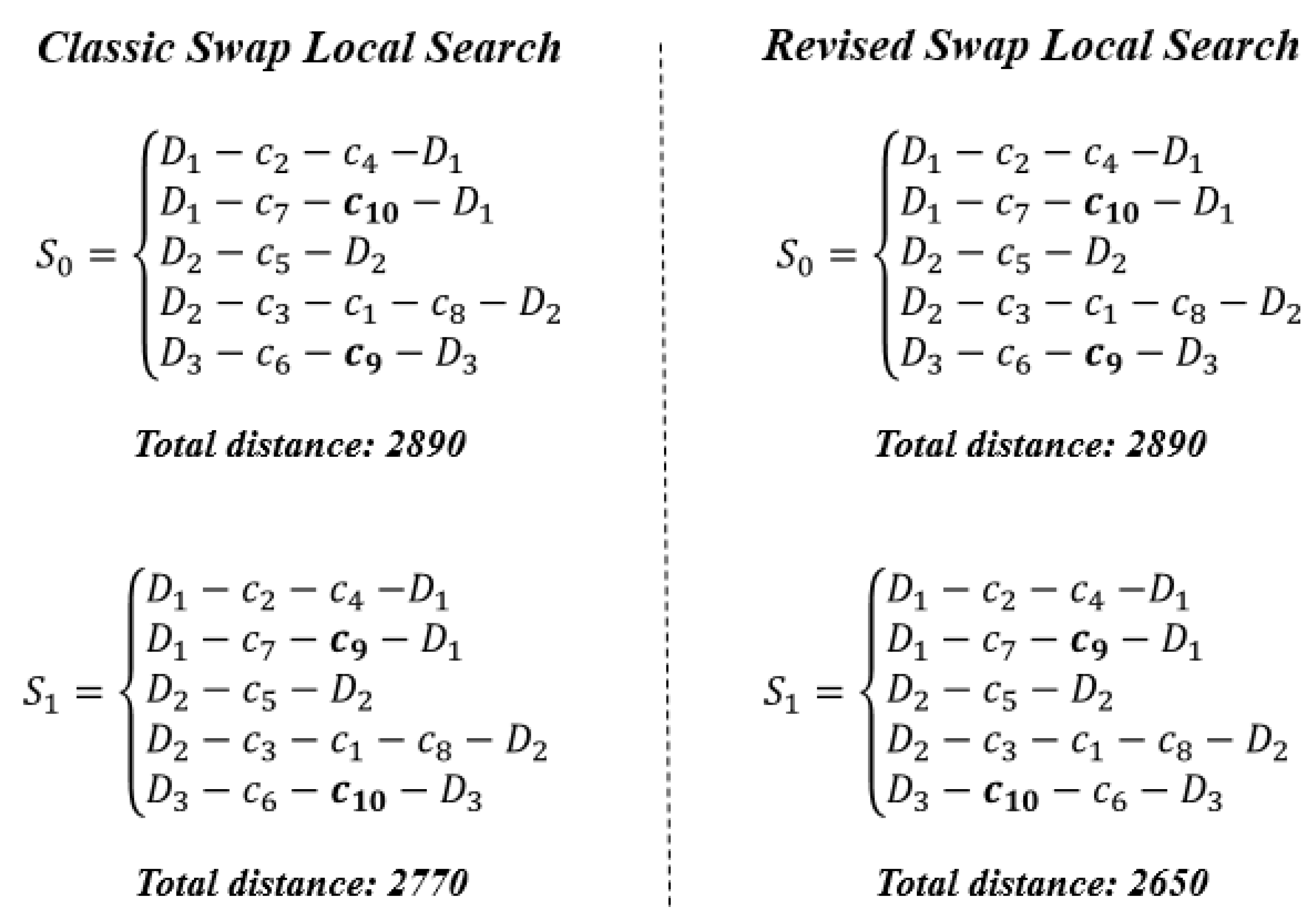
Revised swap local search is a new local search technique proposed in this paper. In the classic swap local search, two selected customers exchange their positions. However, in the revised swap local search, two selected customers exchange their routes and are inserted into the best positions in the new routes.

Figure 2 demonstrates the difference between the classic swap local search and the revised swap local search. In this example, $c_{10}$ and $c_9$ are selected to apply a swap local search. In the classic swap local search, these two customers are exchanged to each other’s positions and the total distance reduces to 2770 from 2890. However, in the revised swap local search, these two customers only exchange their routes, and they are inserted into the best positions on the new routes. Finally, the total distance reduces to 2650. A database is used for reducing CPU (center process unit) time. The database calculates and stores the best position of each customer in each route. When two customers are exchanged, only the affected route is recalculated for the best position of customers from other routes, which helps to reduce CPU time.

4.2.4. MDGVRP Local Search

After generating an ant-solution for MDGVRP, we apply an MDGVRP local search on each MDGVRP solution. In TSACS, we adopt two types of local search: a redundancy removal (RR) local search and a relocate local search. An RR local search is applied twice, before and after a relocate local search. A relocate local search for MDGVRP is similar to the relocate local search for MDVRP in VNS.

Redundant nodes are removed to improve the solution quality. Redundant nodes are nodes which can be removed without making the solution infeasible. The initial solution generated by TSACS contains depots and AFSs as redundant nodes because ants generate GVRP routes from TSP routes in two steps. These redundant nodes can be removed to improve the solution quality.

4.2.5. Update the Trail Intensity

At the end of each iteration, the trail intensities of depot-ants ${\tau }_{ik}^a$ and the trail intensities of route-ants ${\tau }_{ij}^t$ are updated by the best solution found so far. The trail intensities of depot-ants are updated as follows:

$${\tau }_{ik}^{a^{new}} = \alpha \times {\tau }_{ik}^{a^{old}} + \Delta {\tau }_{ik}, \forall i\in C, k \in D$$

(14)

where

$$∆{\tau }_{ik}=\{\begin{array}{l}\frac{1}{l_{ik}}, if customer i is assigned to depot k in the best solution.\\ 0, otherwise.\end{array}$$

(15)

Here, $\alpha$ is the trail persistence and $l_{ik}$ is the distance between customer $i$ and depot $k$. Similarly, route trail intensities are updated as follows:

$${\tau }_{ik}^{t^{old}} = \beta \times {\tau }_{ij}^{t^{old}} + \Delta {\tau }_{ik}, \forall i,j\in V, i\ne j$$

(16)

where

$$∆{\tau }_{ij}=\{\begin{array}{l}\frac{1}{l_{ij}}, if node i and j are connected in the best solution.\\ 0, otherwise.\end{array}$$

(17)

In this way, the trail intensities are updated at the end of each iteration, which guides the artificial ants to find better solutions in the next iteration.

5. Numerical Experiments and Analysis

MDGVRP is a new model; therefore, new problem instances are generated to test the performance of the two algorithms designed for solving MDGVRP. Besides, we also tested our TSACS on the 23 benchmark instances of MDVRP to check the performance of TSACS on MDVRP. All experiment results are reported in the following sections.

We randomly generated 17 small problem instances and 60 large problem instances. The positions of depots, AFSs and customers are randomly generated on one 300-by-300-mile grid. In generating the customer locations. We ensure that a customer can be assigned to, at least, one depot. The tank capacity of vehicles $T$ is 60 gallons, and the fuel consumption rate $r$ is 0.2 gallons/mile. The demand of each customer $q_i \left(\forall i\in C\right)$ is generated between 15 and 25, and the capacity of vehicle $Q$ is set to 300.

These 17 small instances (labeled as MDGVRPT 1 to MDGVRPT 17) consider the number of customers $\left(N\right)$ as 5, 7, 9, 11, 13 and 15; the number of depots $\left(M\right)$ as 2, 3 and 4; and the number of AFSs $\left(NS\right)$ as 2, respectively. Thus, a total of 17 small instances are generated. In large instances (labeled as MDGVRP 1 to MDGVRP 60), the number of customers is 25, 50, 75, 100, 150 and 200; the number of depots is 4, 6 and 8; and the number of AFSs is 2, 4, 6 and 8. Thus, a total of 60 large instances are generated. The small problem instances are used to obtain the optimal solution by solving the mathematical formulation provided in Section 3. The large problem instances are generated to evaluate the relative performance of proposed algorithms. Before testing the instances, all necessary parameters are set as follows

For TSACS, we set the number of iterations $A$ as 1000, the number of artificial ants $y$ as 20, the trail persistence for depot-ants $\alpha$ as 0.95 and trail persistence for route-ants $\beta$ as 0.95. The TSACS stops if, at least, one of the following conditions is satisfied: (1) no better solution found in the last 50 iterations; (2) the solving time has exceeded 7200 s. For the PBA, the rate distinguishing between a borderline and non-borderline customer $r_a$ is set as 0.7.

5.1. Experiment Results and Analysis

The TSACS algorithm and the PBA were coded in C++ and implemented on AMD Opteron 2.3 GHz with 16 GB of RAM. The mathematical formulation is solved using AMPL on a desktop with Intel Core i5-4590 3.3 GHz with 8 GB of RAM. The computing time of the mathematical formulation is affected by the number of dummy vertices. Therefore, we set the number of dummy vertices for each AFS to 2 (3 nodes in total for each AFS) and the maximum number of vehicles is the three times of the number of depots. We also set the maximum solving time as 14,400 s (4 h). All experiment results are provided in the following sections.

5.2. Experiments on Small-Size Instances

The purpose of small-size instances is to evaluate the absolute performance of the proposed algorithm. We use a formulation described in Section 3 to obtain the optimal solution. We report MDGVRP CO₂ emissions (kg) and the CPU time (seconds) used to solve the instance and Percentage Gap (PG) from the optimal solution for the proposed TSACS algorithm and the PBA. The results are shown in

Table 1. Experiment results of small-sized instance.

Instance	N	NS	M	CPLEX		PBA			TSACS
				Optimal	CPU	CO2	CPU	PG (%)	CO2	CPU	PG (%)
				Solution	Time	Emissions	Time		Emissions	Time
				(kg)	(Seconds)	(kg)	(Seconds)		(kg)	(Seconds)
MDGVRPT1	5	2	2	179.24	0.22	134.87	<1	50.48	179.24	60.12	0.00
MDGVRPT2	7	2	2	191.08	0.52	143.27	<1	49.96	191.08	122.88	0.00
MDGVRPT3	9	2	2	205.7	19.86	194.80	<1	89.39	205.7	121.25	0.00
MDGVRPT4	11	2	2	214.94	190.38	170.22	<1	58.39	214.94	142.27	0.00
MDGVRPT5	13	2	2	235.26	863.11	224.93	<1	91.22	235.26	382.06	0.00
MDGVRPT6	15	2	2	265.00	6012.00	343.61	<1	159.34	265.00	272.13	0.00
MDGVRPT7	5	2	3	163.88	0.35	118.26	<1	44.33	163.88	91.44	0.00
MDGVRPT8	7	2	3	173.46	0.31	123.05	<1	41.88	173.46	96.33	0.00
MDGVRPT9	9	2	3	198.14	0.74	99.07	<1	0.00	198.14	147.45	0.00
MDGVRPT10	11	2	3	205.42	3.62	102.71	<1	0.00	205.42	120.48	0.00
MDGVRPT11	13	2	3	215.62	4.69	109.52	<1	1.58	215.62	134.35	0.00
MDGVRPT12	15	2	3	261.18	12907.60	134.38	<1	2.90	261.18	178.07	0.00
MDGVRPT13	5	2	4	137.44	0.28	76.40	<1	11.17	137.44	108.31	0.00
MDGVRPT14	7	2	4	170.90	0.37	85.45	<1	0.00	170.90	127.27	0.00
MDGVRPT15	9	2	4	178.22	0.90	89.11	<1	0.00	178.22	137.90	0.00
MDGVRPT16	11	2	4	186.94	1.47	97.82	<1	4.66	186.94	148.22	0.00
MDGVRPT17	13	2	4	232.50	31.22	120.91	<1	4.01	232.50	199.37	0.00
Average				200.88	1178.68	139.32	<1	35.84	200.88	152.35	0.00

.

The results reported in Table 1 show that the average carbon emissions for the solution obtained by CPLEX, PBA and TSACS are 200.88, 139.32 and 200.88, respectively. The proposed TSACA is able to find the optimal solution for all small-sized instances with an average PG of 0.0 %. The PBA obtained the optimal solution for only four instances, and the average PG between the PBA solution and the optimal solution is 35.84%. The PG for MDGVRPT6 is 159.34%, which indicates that the solution quality of the PBA is not as good as that of TSACS for small-size instances.

From Table 1, it can be seen that TSACS can find the optimal solution for all small-sized instances in 152.35 s on average, which is much less than the 1178.68 s spent by CPLEX. It can also be observed that, when the problem size increases, the CPU time of CPLEX rises dramatically. We could not solve the instance for more than 15 customers.

5.3. Experiments on Large-Size Instances

The optimal solution cannot be obtained for a larger size problem. Therefore, Relative Percentage Deviation (RPD) is used to evaluate the performance of the TSACS and PBA. For the $j^{th}$ instance and $i^{th}$ algorithm, the $RP{D}_{ij}$ is calculated based on the following Equation (18):

$$RP{D}_{ij} = \frac{(H_j^i-B_j)}{B_j}\times 100 \%$$

(18)

In this formula, $H_j^i$ stands for the solution obtained by the $i^{th}$ algorithm for the $j^{th}$ instance and $B_j$ represents the best solution from all evaluated algorithms for the $j^{th}$ problem instance. The results of large instances are shown in

Table 2. Experiment results of large-sized instance.

Instance	n	NS	M	PBA			TSACS
				CO2	CPU	RPD (%)	CO2	CPU	RPD (%)
				Emissions	Time		Emissions	Time
				(kg)	(Seconds)		(kg)	(Seconds)
MDGVRP1	25	2	4	463.76	<1	42.74	324.90	399.27	0.00
MDGVRP2	50	2	4	1075.60	<1	115.18	499.86	2618.04	0.00
MDGVRP3	100	2	4	1693.78	<1	135.88	718.06	7340.48	0.00
MDGVRP4	150	2	4	1589.30	<1	67.44	949.14	7685.46	0.00
MDGVRP5	200	2	4	2087.56	<1	84.94	1128.80	8131.56	0.00
MDGVRP6	25	4	4	440.40	<1	47.33	298.92	505.90	0.00
MDGVRP7	50	4	4	1170.16	<1	173.45	427.94	1877.21	0.00
MDGVRP8	100	4	4	1502.32	<1	125.96	664.86	7345.99	0.00
MDGVRP9	150	4	4	1594.28	<1	84.98	861.86	7219.72	0.00
MDGVRP10	200	4	4	2537.36	<1	144.01	1039.84	8244.57	0.00
MDGVRP11	25	6	4	465.40	<1	68.47	276.24	393.49	0.00
MDGVRP12	50	6	4	982.90	<1	142.45	405.40	3187.19	0.00
MDGVRP13	100	6	4	1520.04	<1	149.00	610.46	7222.02	0.00
MDGVRP14	150	6	4	1679.14	<1	114.56	782.58	7391.53	0.00
MDGVRP15	200	6	4	2041.48	<1	110.09	971.70	7903.02	0.00
MDGVRP16	25	8	4	466.72	<1	88.36	247.78	1433.36	0.00
MDGVRP17	50	8	4	1066.32	<1	169.07	396.30	2806.09	0.00
MDGVRP18	100	8	4	1785.90	<1	200.37	594.56	7246.79	0.00
MDGVRP19	150	8	4	1764.42	<1	128.75	771.34	7757.41	0.00
MDGVRP20	200	8	4	2667.78	<1	164.89	1007.14	7456.24	0.00
MDGVRP21	25	2	6	386.92	<1	47.10	263.02	477.99	0.00
MDGVRP22	50	2	6	1099.32	<1	184.28	386.70	1619.00	0.00
MDGVRP23	100	2	6	1811.32	<1	203.92	595.98	7353.46	0.00
MDGVRP24	150	2	6	1901.96	<1	148.00	766.92	7396.85	0.00
MDGVRP25	200	2	6	2778.32	<1	189.23	960.58	7855.72	0.00
MDGVRP26	25	4	6	393.04	<1	44.31	272.36	464.29	0.00
MDGVRP27	50	4	6	1274.18	<1	220.38	397.70	3391.48	0.00
MDGVRP28	100	4	6	2173.80	<1	254.66	612.94	7303.76	0.00
MDGVRP29	150	4	6	1716.94	<1	121.36	775.62	7320.43	0.00
MDGVRP30	200	4	6	3085.10	<1	230.90	932.32	8408.52	0.00
MDGVRP31	25	6	6	430.02	<1	53.98	279.26	507.75	0.00
MDGVRP32	50	6	6	1006.88	<1	160.30	386.82	2322.16	0.00
MDGVRP33	100	6	6	1748.42	<1	201.45	580.00	7207.18	0.00
MDGVRP34	150	6	6	2277.22	<1	195.30	771.16	7429.96	0.00
MDGVRP35	200	6	6	3523.10	<1	286.43	911.70	7794.60	0.00
MDGVRP36	25	8	6	454.68	<1	56.40	290.72	523.12	0.00
MDGVRP37	50	8	6	1144.40	<1	200.35	381.02	3515.85	0.00
MDGVRP38	100	8	6	1528.70	<1	167.21	572.10	7292.39	0.00
MDGVRP39	150	8	6	3461.22	<1	352.02	765.72	7849.12	0.00
MDGVRP40	200	8	6	3777.16	<1	310.83	919.40	7931.12	0.00
MDGVRP41	25	2	8	372.52	<1	36.77	272.36	535.77	0.00
MDGVRP42	50	2	8	663.88	<1	74.61	380.22	3371.60	0.00
MDGVRP43	100	2	8	1379.12	<1	134.19	588.88	7333.87	0.00
MDGVRP44	150	2	8	1528.78	<1	120.10	694.58	7536.94	0.00
MDGVRP45	200	2	8	1728.32	<1	95.26	885.16	7431.36	0.00
MDGVRP46	25	4	8	347.78	<1	24.53	279.26	714.04	0.00
MDGVRP47	50	4	8	695.28	<1	84.77	376.30	4151.57	0.00
MDGVRP48	100	4	8	1072.64	<1	87.19	573.02	7376.03	0.00
MDGVRP49	150	4	8	1628.78	<1	127.70	715.32	7289.29	0.00
MDGVRP50	200	4	8	2248.40	<1	163.14	854.46	8277.40	0.00
MDGVRP51	25	6	8	377.38	<1	29.81	290.72	779.23	0.00
MDGVRP52	50	6	8	694.36	<1	77.23	391.78	3603.41	0.00
MDGVRP53	100	6	8	994.58	<1	74.01	571.56	7422.09	0.00
MDGVRP54	150	6	8	2040.60	<1	182.67	721.90	7353.37	0.00
MDGVRP55	200	6	8	2247.88	<1	147.78	907.22	8621.59	0.00
MDGVRP56	25	8	8	390.58	<1	35.86	287.50	692.14	0.00
MDGVRP57	50	8	8	699.98	<1	90.04	368.34	3765.78	0.00
MDGVRP58	100	8	8	1094.10	<1	97.08	555.18	7256.76	0.00
MDGVRP59	150	8	8	1770.98	<1	152.99	700.02	7681.20	0.00
MDGVRP60	200	8	8	2072.12	<1	131.56	894.86	8939.63	0.00
Average				1476.92	<1	132.56	601.80	5304.39	0.00

.

In Table 2, it is clear that the quality of solutions generated by TSACS is much better than that of PBA. The RPD of TSACS is 0.00% for all problem instances, which means that TSACS can obtain a better solution for all problem instances. The average RPD of PBA is 132.56%, which indicates that the solution of PBA is 132.56% worse, on average, than that of TSACS. In addition, the solution quality of PBA is very “unstable”. For some instances, such as MDGVRP46 and MDGVRP51, PBA can get relatively high-quality solutions. However, for most of the other instances, the solution quality of PBA is unsatisfactory. The PBA can solve all instances faster. For TSACS, the solving time increases with the size of each instance. In fact, for TSACS, solution quality and CPU time are correlated. The CPU time can be shortened by decreasing the number of iterations or by reducing the number of artificial ants. However, decreasing the CPU time decreases the solution quality. Therefore, a trade-off analysis is performed to fix the number of iterations and the number of ants.

5.4. Experiments on MDVRP Instances

MDGVRP is a variant of MDVRP. Thus, the proposed algorithm can also be used to solve MDVRP. There are 23 benchmark instances for MDVRP extracted from previous literature. All these 23 benchmark instances and best-known solutions are available at http://neo.lcc.uma.es/vrp/vrp-instances/multiple-depot-vrp-instances/. The proposed TSACS is compared with the FIND algorithm [30], CGL method [31], a standard ACO [25], ACO with the ant-weight strategy and the mutation operation (ACO-WM) [32], the PIACO method [6], the HGSADC algorithm [5], and ELTG [22]. For solving the MDVRP problem, we set our objective function as a minimization of total distances because existing algorithms minimize the total travel distance. We set carbon emission conversion factor (CCF) to 1 while solving the problem with the total travel distance objective function.

The experimental results and related RPD of different algorithms are provided in the

Table 3. The results of TSACS compared with other heuristic methods.

Ins	Best-Known Solutions	FIND		CGL		ACO		ACO-WM		PIACO		HGSADC		ELTG		TSACS
		Best	RPD	Best	RPD	Best	RPD	Best	RPD	Best	RPD	Best	RPD	Best	RPD	Best	RPD
1	576.86	576.86	0.00	576.86	0.00	576.86	0.00	576.86	0.00	576.86	0.00	576.86	0.00	576.86	0.00	576.86	0.00
2	473.53	473.53	0.00	473.53	0.00	484.28	2.27	473.53	0.00	473.53	0.00	473.53	0.00	473.53	0.00	473.53	0.00
3	641.18	641.18	0.00	645.15	0.62	645.15	0.62	641.18	0.00	641.18	0.00	641.18	0.00	641.18	0.00	641.18	0.00
4	1001.04	1003.86	0.28	1006.66	0.56	1020.52	1.95	1001.49	0.04	1001.49	0.04	1001.04	0.00	1001.04	0.00	1010.57	0.95
5	750.03	750.26	0.03	753.4	0.45	750.26	0.03	750.26	0.03	750.26	0.03	750.03	0.00	750.03	0.00	751.154	0.15
6	876.5	876.5	0.00	877.84	0.15	878.34	0.21	876.5	0.00	876.5	0.00	876.5	0.00	876.5	0.00	880.574	0.46
7	881.97	892.58	1.20	891.95	1.13	898.8	1.91	887.11	0.58	885.69	0.42	881.97	0.00	884.66	0.30	881.97	0.00
8	4371.66	4485.08	2.59	4482.44	2.53	4508.14	3.12	4500.15	2.94	4482.38	2.53	4372.78	0.03	4371.66	0.00	4516.75	3.32
9	3858.66	3937.81	2.05	3920.85	1.61	4083.44	5.83	3913	1.41	3912.23	1.39	3858.66	0.00	3880.55	0.57	3939.52	2.10
10	3629.6	3669.38	1.10	3714.65	2.34	3747.62	3.25	3693.4	1.76	3663	0.92	3631.11	0.04	3629.6	0.00	3724.93	2.63
11	3545.48	3648.94	2.92	3580.84	1.00	3599.93	1.54	3564.74	0.54	3554.08	0.24	3546.06	0.02	3545.48	0.00	3624.67	2.23
12	1318.95	1318.95	0.00	1318.95	0.00	1327	0.61	1318.95	0.00	1318.95	0.00	1318.95	0.00	1318.95	0.00	1318.95	0.00
13	1318.95	1318.95	0.00	1318.95	0.00	1318.95	0.00	1318.95	0.00	1318.95	0.00	1318.95	0.00	1318.95	0.00	1318.95	0.00
14	1360.12	1365.68	0.41	1360.12	0.00	1375.22	1.11	1373.18	0.96	1365.68	0.41	1360.12	0.00	1360.12	0.00	1360.12	0.00
15	2505.29	2551.45	1.84	2534.13	1.15	2588.22	3.31	2565.67	2.41	2551.45	1.84	2505.29	0.00	2505.29	0.00	2505.29	0.00
16	2572.23	2572.23	0.00	2572.23	0.00	2604.9	1.27	2572.23	0.00	2572.23	0.00	2572.23	0.00	2572.23	0.00	2572.23	0.00
17	2708.99	2731.37	0.83	2720.23	0.41	2776.99	2.51	2708.99	0.00	2708.99	0.00	2708.99	0.00	2708.99	0.00	2708.99	0.00
18	3702.75	3781.03	2.11	3710.49	0.21	3907.88	5.54	3846.05	3.87	3781.03	2.11	3702.75	0.00	3702.75	0.00	3749.34	1.26
19	3827.06	3827.06	0.00	3827.06	0.00	3863.03	0.94	3827.06	0.00	3827.06	0.00	3827.06	0.00	3827.06	0.00	3827.06	0.00
20	4058	4097.06	0.96	4058	0.00	4231.28	4.27	4142	2.07	4097.06	0.96	4058	0.00	4058	0.00	4058	0.00
21	5474.74	5656.46	3.32	5535.99	1.12	5579.86	1.92	5495.54	0.38	5474.74	0.00	5474.74	0.00	5474.74	0.00	5619.95	2.65
22	5702.06	5718	0.28	5716.01	0.24	5897.64	3.43	5832.07	2.28	5772.23	1.23	5702.06	0.00	5702.06	0.00	5702.06	0.00
23	6078.75	6145.58	1.10	6139.73	1.00	6341.61	4.32	6183.13	1.72	6125.58	0.77	6078.75	0.00	6095.46	0.27	6078.75	0.00
Average			0.91		0.63		2.17		0.91		0.56		0.00		0.05		0.68

. Additionally, as mentioned in [6], the run times are not only dependent on the CPU of the computers but also on the operation system (OS), compiler, programming language and the precision used during the execution of the run. Therefore, the comparison of CPU time is not included.

From Table 3, it can be seen that HGSADC has the best performance, followed by ELTG, PIACO, TSACS, CGL, FIND, ACO-WM and ACO. The average RPD of TSACS is only 0.68%, which is the 5th best among all algorithms, and TSACS can match the existing best-known solution for 14 instances, which is 3rd among all algorithms. The experimental results on MDVRP instances proved that TSACS can solve MDGVRP problems as well as MDGVRP variant problems with acceptable solution quality.

5.5. Comparative Evaluation of the Proposed Algorithms

This paper solves the MDGVRP problem using three methods: (1) the mathematical model, (2) the PBA, and (3) TSACS algorithm. The mathematical model is solved by AMPL software using CPLEX solver. The main advantage of the mathematical model is its ability to obtain the optimal solution. However, the CPU time used by the mathematical model increases exponentially when problem size (in terms of N, NS and M) increases linearly. Thus, the mathematical model becomes impractical for solving bigger problem instances. The biggest problem solved by our mathematical model has only 11 customers, three AFVs and four depots. The PBA falls under the category of the heuristic algorithm. The main advantage of the PBA is the use of less CPU time. The PBA is able to solve the problem in less than one second for all the instances, including instances with 200 customers. The main disadvantage of the PBA is the poor solution quality produced by the algorithm. The PBA is, on average, 35% worse than the optimal solution, even for small problem instances. The TSACS algorithm falls under the category of metaheuristic. The TSACS algorithm is a compromise method between the mathematical model and the heuristic algorithm. The TSACS has an advantage over mathematical model for solving bigger problem instances but it cannot guarantee optimal solution. The TSACS has an advantage over the PBA for producing better quality solution but it takes more CPU time.

6. Conclusions

Recently, multi-national transportation companies have been focusing more on environmental sustainability performance. In this paper, the Multi-Depot Green Vehicle Routing Problem (MDGVRP) is addressed. In MDGVRP, the Alternative Fuel-powered Vehicles (AFVs) are used to deliver goods to customers. These AFVs depart from different depots, serve customers, and, at the end, return back to their original depots. In the service process, AFVs need to consider the remaining fuel level and the remaining cargo level. We provide mathematical formulation to model the MDGVRP problem with the aim of minimizing the total carbon emissions of fleet operation.

We proposed two algorithms, the Two-stage Ant Colony System (TSACS) Algorithm and the Partition-Based Algorithm (PBA) to solve MDGVRP. We generated 17 small-size instances and 60 large-size instances to test the performance of the TSACS algorithm and the PBA. The experimental results reveal that although the PBA can solve each instance within 1 s, the solution quality is unsatisfactory. However, TSACS has a very good overall performance on solution quality. The average carbon emissions for 18 small problem instances is 200.88 kg for both CPLEX and the TSACS algorithm, which indicates that proposed TSACS is able to achieve optimal solution for all small problem instances. TSACS is able to obtain the best solution for all 18 small-sizes instances in 155.18 s on average.

The experimental results of TSACS on the benchmark instances of MDVRP prove that TSACS can also be used to solve variants of MDGVRP problems. These results indicate that the ant colony algorithm can effectively solve the MDGVRP problem. In the future, the proposed ideas may be implemented for testing the performance for solving other variants of combinatorial optimization problems in logistics and supply management [33]. Moreover, with the development of alternative fuel-powered vehicles and a growing concern for environmental protection, we believe that the research on MDGVRP can be applied to other types of VRP with additional social-consideration-type constraints.

References

- Erdoğan, S.; Miller-Hooks, E. A green vehicle routing problem. Transp. Res. Part E Logist. Transp. Rev. 2012, 48, 100–114. [Google Scholar] [CrossRef]
- Lin, C.; Choy, K.L.; Ho, G.T.; Chung, S.H.; Lam, H. Survey of green vehicle routing problem: Past and future trends. Expert Syst. Appl. 2014, 41, 1118–1138. [Google Scholar] [CrossRef]
- Schneider, M.; Stenger, A.; Goeke, D. The electric vehicle-routing problem with time windows and recharging stations. Transp. Sci. 2014, 48, 500–520. [Google Scholar] [CrossRef]
- Montoya-Torres, J.R.; Franco, J.L.; Isaza, S.N.; Jiménez, H.F.; Herazo-Padilla, N. A literature review on the vehicle routing problem with multiple depots. Comput. Ind. Eng. 2015, 79, 115–129. [Google Scholar] [CrossRef]
- Vidal, T.; Crainic, T.G.; Gendreau, M.; Lahrichi, N.; Rei, W. A hybrid genetic algorithm for multidepot and periodic vehicle routing problems. Oper. Res. 2012, 60, 611–624. [Google Scholar] [CrossRef]
- Yu, B.; Yang, Z.; Xie, J. A parallel improved ant colony optimization for multi-depot vehicle routing problem. J. Oper. Res. Soc. 2011, 62, 183–188. [Google Scholar] [CrossRef]
- Farneti, F.; Guthrie, J. Sustainability Reporting by Australian Public Sector Organisations: Why They Report; Accounting Forum; Taylor, Francis: Abingdon, UK, 2009; pp. 89–98. [Google Scholar]
- Morhardt, J.E.; Baird, S.; Freeman, K. Scoring corporate environmental and sustainability reports using GRI 2000, ISO 14031 and other criteria. Corp. Soc. Resp. Environ. Manag. 2002, 9, 215–233. [Google Scholar] [CrossRef]
- Kaabachi, I.; Jriji, D.; Krichen, S. An improved ant colony optimization for green multi-depot vehicle routing problem with time windows. In Proceedings of the 2017 18th IEEE/ACIS International Conference on Software Engineering, Artificial Intelligence, Networking and Parallel/Distributed Computing (SNPD) IEEE, Kanazawa, Japan, 26–28 June 2017; pp. 339–344. [Google Scholar]
- Jabir, E.; Panicker, V.V.; Sridharan, R. Design and development of a hybrid ant colony-variable neighbourhood search algorithm for a multi-depot green vehicle routing problem. Transp. Res. Part D Transp. Environ. 2017, 57, 422–457. [Google Scholar] [CrossRef]
- Li, J.; Wang, R.; Li, T.; Lu, Z.; Pardalos, P.M. Benefit analysis of shared depot resources for multi-depot vehicle routing problem with fuel consumption. Transp. Res. Part D Transp. Environ. 2018, 59, 417–432. [Google Scholar] [CrossRef]
- Wang, Y.; Assogba, K.; Fan, J.; Xu, M.; Liu, Y.; Wang, H. Multi-depot green vehicle routing problem with shared transportation resource: Integration of time-dependent speed and piecewise penalty cost. J. Clean. Prod. 2019, 232, 12–29. [Google Scholar] [CrossRef]
- Felipe, Á.; Ortuño, M.T.; Righini, G.; Tirado, G. A heuristic approach for the green vehicle routing problem with multiple technologies and partial recharges. Transp. Res. Part E Logist. Transp. Rev. 2014, 71, 111–128. [Google Scholar] [CrossRef]
- Montoya, A.; Guéret, C.; Mendoza, J.E.; Villegas, J.G. A multi-space sampling heuristic for the green vehicle routing problem. Transp. Res. Part C Emerg. Technol. 2016, 70, 113–128. [Google Scholar] [CrossRef]
- Koç, Ç.; Karaoglan, I. The green vehicle routing problem: A heuristic based exact solution approach. Appl. Soft Comput. 2016, 39, 154–164. [Google Scholar]
- Zhang, S.; Gajpal, Y.; Appadoo, S. A meta-heuristic for capacitated green vehicle routing problem. AnOR 2017, 269, 753–771. [Google Scholar] [CrossRef]
- Andelmin, J.; Bartolini, E. An exact algorithm for the green vehicle routing problem. Transp. Sci. 2017, 51, 1288–1303. [Google Scholar] [CrossRef]
- Peng, B.; Zhang, Y.; Gajpal, Y.; Chen, X. A Memetic Algorithm for the Green Vehicle Routing Problem. Sustainability 2019, 11, 6055. [Google Scholar] [CrossRef] [Green Version]
- Nocera, S.; Ruiz-Alarcón-Quintero, C.; Cavallaro, F. Assessing carbon emissions from road transport through traffic flow estimators. Transp. Res. Part C Emerg. Technol. 2018, 95, 125–148. [Google Scholar] [CrossRef]
- Fu, M.; Kelly, J.A.; Clinch, J.P. Estimating annual average daily traffic and transport emissions for a national road network: A bottom-up methodology for both nationally-aggregated and spatially-disaggregated results. J. Transp. Geogr. 2017, 58, 186–195. [Google Scholar] [CrossRef]
- Cassidy, P.; Bennett, H. TRAMP—A multi-depot vehicle scheduling system. J. Oper. Res. Soc. 1972, 23, 151–163. [Google Scholar] [CrossRef]
- Escobar, J.W.; Linfati, R.; Toth, P.; Baldoquin, M.G. A hybrid granular tabu search algorithm for the multi-depot vehicle routing problem. JHeu 2014, 20, 483–509. [Google Scholar] [CrossRef]
- Nagy, G.; Salhi, S. Heuristic algorithms for single and multiple depot vehicle routing problems with pickups and deliveries. Eur. J. Oper. Res. 2005, 162, 126–141. [Google Scholar] [CrossRef] [Green Version]
- Reichmuth, D.S.; Lutz, A.E.; Manley, D.K.; Keller, J.O. Comparison of the technical potential for hydrogen, battery electric, and conventional light-duty vehicles to reduce greenhouse gas emissions and petroleum consumption in the United States. Int. J. Hydrog. Energy 2013, 38, 1200–1208. [Google Scholar] [CrossRef]
- Dorigo, M.; Maniezzo, V.; Colorni, A. Ant system: Optimization by a colony of cooperating agents. IEEE Trans. Syst. Man. Cybern. B 1996, 26, 29–41. [Google Scholar] [CrossRef] [PubMed] [Green Version]
- Bell, J.E.; McMullen, P.R. Ant colony optimization techniques for the vehicle routing problem. Adv. Eng. Inform. 2004, 18, 41–48. [Google Scholar] [CrossRef]
- Gambardella, L.M.; Montemanni, R.; Rizzoil, A.E.; Lucibello, E. Ant colony optimization for real-world vehicle routing from theory to applications. Swarm Intell. 2007, 1, 135–151. [Google Scholar]
- Gajpal, Y.; Abad, P. An ant colony system (ACS) for vehicle routing problem with simultaneous delivery and pickup. Comput. Oper. Res. 2009, 36, 3215–3223. [Google Scholar] [CrossRef]
- Ting, C.; Chen, C. A multiple ant colony optimization algorithm for the capacitated location routing problem. Intern. J. Prod. Econ. 2013, 141, 34–44. [Google Scholar] [CrossRef]
- Renaud, J.; Laporte, G.; Boctor, F.F. A tabu search heuristic for the multi-depot vehicle routing problem. Comput. Oper. Res. 1996, 23, 229–235. [Google Scholar] [CrossRef]
- Cordeau, J.F.; Gendreau, M.; Laporte, G. A tabu search heuristic for periodic and multi-depot vehicle routing problems. Networks 1997, 30, 105–119. [Google Scholar] [CrossRef]
- Yu, B.; Yang, Z.Z.; Yao, B.Z. An improved ant colony optimization for vehicle routing problem. Eur. J. Opl. Res. 2009, 196, 171–176. [Google Scholar] [CrossRef]
- Zhou, R.; Liao, Y.; Shen, W. Channel selection and fulfillment service contracts in the presence of asymmetric service information. Int. J. Prod. Econ. 2019, 222, 107504. [Google Scholar] [CrossRef]
Figure 1.
Process of generating Green Vehicle Routing Problem (GVRP) routes for depot .
Figure 2.
Comparison between the classic swap local search and the revised swap local search.