Article

Assessment of the Variability of Air Pollutant Concentrations at Industrial, Traffic and Urban Background Stations in Krakow (Poland) Using Statistical Methods

Department of Environmental Management and Protection, Faculty of Mining Surveying and Environmental Engineering, AGH University of Science and Technology, 30-059 Krakow, Poland
*
Author to whom correspondence should be addressed.
Sustainability 2021, 13(10), 5623; https://0-doi-org.brum.beds.ac.uk/10.3390/su13105623
Submission received: 19 April 2021 / Revised: 12 May 2021 / Accepted: 17 May 2021 / Published: 18 May 2021

Abstract

:
In cities with an extensive air quality monitoring (AQM) system, the results of pollutant concentration measurements obtained in this system can be used not only for current assessments of air pollution, but also for analyzes aimed at better identification of factors influencing the air quality and for tracking trends in changes taking place in this regard. This can be achieved with the use of statistical methods that allow for the assessment of the variability of measurement data observed at stations of various types and for the determination of possible interdependencies between these data. In this article, an analysis of this type was carried out for traffic, urban background and industrial AQM stations in Krakow (Southern Poland) operating in the years 2017–2018 with the use of, i.a., cluster analyzes, as well as dependent samples t-test and Wilcoxon signed-rank test, taking into account the concentrations of air pollutants such as fine particulate matter (PM10), nitrogen dioxide (NO2), benzene (C6H6) and sulfur dioxide (SO2). On the basis of the conducted analyzes, similarities and differences were shown between the data observed at individual types of stations, and the possibilities of using them to identify the causes of the observed changes and the effects of remedial actions to improve air quality undertaken recently and planned in the future were indicated. It was found that the air concentrations of some substances measured at these stations can be used to assess the emission abatement effects in road transport (NO2, PM10 or C6H6), residential heating (PM10 or SO2), and selective industrial plants (SO2, NO2 or C6H6).

1. Introduction

Air quality in urban-industrial areas is determined primarily by the emission of pollutants from, residential, traffic and industrial sources as well as meteorological and topographic factors influencing transport, dispersion and conversions of pollutants in the atmospheric air. The assessment of the contribution of particular types of sources to the level of pollutant concentrations in the air is usually very labor intensive. It requires a detailed inventory of all significant emission sources influencing the air quality in a given region (along with the determination of the amount of pollutants emitted from individual sources and its temporal variability), as well as determination of the concentrations caused by individual emission sources, which is most commonly carried out using deterministic models that allow to simulate the transport and dispersion of pollutants [1,2,3]. It is also possible to apply receptor modeling allowing, among others, for the assessment of the contribution of natural and other emission sources located at greater distances, not usually included in modeling carried out with the use of deterministic models, as this would require balancing the emission over a larger area and the application of regional and mesoscale meteorological and dispersion models [4,5,6]. Receptor models are most often based on the results of measurements of meteorological parameters, concentrations of various air pollutants as well as the chemical composition and/or physical characteristics of the atmospheric aerosol, which usually involves carrying out a specially planned measurement program [6,7]. On the other hand, machine learning methods and regression modeling are increasingly used to solve various problems in the field of assessing spatial variability and forecasting the air pollution [8,9,10,11].
Considering the complexity of factors influencing air quality and generally high uncertainty of the results of emission estimation and mathematical modeling, the most reliable information about the air pollution is provided by the results of direct measurements. They are typically carried out using reference measurement method or methods recognized as equivalent to the reference [12]. The suitability of air quality monitoring stations for the performance of specific tasks can be assessed using various methods, depending mainly on the type of station (which is strongly conditioned by its location and spatial representativeness), size or specificity of the monitored area and measurement range [13,14,15,16].
Basically, in urban-industrial areas there are three main types of monitoring stations: urban background stations, traffic stations and industrial stations. The measurement data obtained from them usually allows for the assessment of the average exposure to air pollution in the city, the impact of road transport and the impact of industry, respectively. These impacts, however, overlap each other and depending on the location of the station, the wind direction and the period assessed, they may, to a lesser or greater extent, reflect different types of emission sources as well as the local and inflow background [17,18,19,20,21,22,23,24].
The variability assessment of the measurement results of pollutant concentrations in the air at various types of monitoring stations was carried out, among others, in research works [25,26,27,28,29,30,31,32,33,34,35,36,37,38,39,40]. In some cases, it was performed with the use of cluster analysis or other data mining techniques and statistical methods. Numerous applications of cluster analysis were described in [41]. Moreover, in [42] the similarity assessment of air quality monitoring stations on the basis of PM2.5 concentrations enabled detecting redundant stations. In [43] the clustering of diurnal concentration profiles of PM10 and black carbon was conducted. Statistical significance tests (including, for example, dependent samples t-test or its non-parametric equivalent–Wilcoxon signed-rank test) were also conducted in air quality studies. For example, in [44] Wilcoxon signed-rank test allowed to assess the statistical significance of the differences between indoor and outdoor PM10 concentrations. Battista et al. [45] used probability distribution, Kurtosis, Skewness, Poincaré sections and cross-correlation of the different pollutants to assess the air pollution level in the city of Rome and the correlation of anthropogenic sources with the pollutant emission. Statistical analysis of spatiotemporal heterogeneity of the distribution of air quality index (using the Kruskal–Wallis rank-sum test method and the Wilcoxon signed-rank test) was also carried out for urban zones by Zhao et al. [46]. On the other hand, Nikolopoulos et al. [47] used statistical and entropy methods for the investigation of a 17 year PM10 time series recorded from air quality stations in Athens in order to delineate existing stochastic and self-organization trends.
The main goal of this study is a statistical analysis of the degree of variability and interdependence between the concentrations of selected air pollutants (PM10, NO2, C6H6 and SO2) observed in the period of 2017–2018 at three types of air quality monitoring stations in the city of Krakow (Southern Poland): industrial (2 stations), traffic (2 stations) and urban background (4 stations). Krakow, for a city with a population of less than 1 million, is characterized by a fairly extensive network of air quality monitoring. This is partly due to the poor air quality observed for many years, and on the other hand, from the need to monitor changes resulting from the remedial actions taken, related to the elimination of household stoves fired with solid fuels and the thermo-modernization of buildings, the use of renewable energy sources, improved public transport, optimization of street cleaning, modernization of flue gas cleaning systems in combined heat and power plants and the exclusion of the most onerous technologies in the steelworks operating in Krakow [48,49,50,51,52,53,54,55]. The analyzed period (2017–2018) may be a good reference point for further comparative research aimed at assessing the effects of actions taken to improve air quality in Krakow (including the prohibition of using solid fuels with effect from September 2019) or lockdowns resulting from the COVID-19 pandemic.
Statistical analyzes and tests performed in this work (including cluster analysis, dependent samples t-test and Wilcoxon signed-rank test) have not yet been applied to such an extent in relation to data from the public air quality monitoring system in Krakow. The results of air quality measurements in Krakow from the public monitoring system, possibly supplemented with additional measurement data and analyzes, were previously used mainly for the assessment of temporal and spatial variability of air pollution, the identification of emission sources and other factors influencing the level of concentrations of pollutants or their mutual correlation, the estimation of the impact of air pollutants on the health of residents, as well as the assessment or development of deterministic and statistical (stochastic) air quality models.
In works [56,57] the correlation analyses and the dependent samples t-test was used, with respect to PM10 concentration data, in suitability analysis of established in 2016 and 2017 air quality monitoring stations in Krakow (after a significant expansion made in 2015–2017 in the field of PM10 concentration measurements). Using statistical methods, the impact of meteorological factors on air quality in Krakow was also assessed [58,59,60,61,62,63,64] and source apportionment analyzes were performed based on the principal component analysis (PCA) [24,65,66,67] or the positive matrix factorization (PMF) receptor model [68,69,70,71]. Previously, a comprehensive source apportionment analysis for measurements from January–February 2005 was performed by the JRC Institute for Environment and Sustainability using seven multivariate receptor models [72,73].
Moreover, many other studies present long-term trends in changes of air pollutants concentrations in Krakow and their impact on health [74,75,76,77,78,79,80,81,82], the mineralogical composition and microbiological characteristics of aerosols [83,84], the oxidative potential of PM10 and PM2.5 [85], the chemical composition of street dust [86] and dry and wet deposition [87,88,89]. The results of measurements from the automatic air quality monitoring station in Krakow were also used to prepare the pollution background necessary in the process of air pollution modeling and the assessment or validation of the dispersion [90,91,92,93,94,95,96,97] or prognostic [98,99,100,101] models used.
As it results from the previous publications and analyzes of available monitoring data, the air pollution in Krakow in the last 30 years fluctuated under the influence of various meteorological conditions and the activity of emission sources but is generally characterized by a downward trend [74,82]. A dozen or so years ago, the combustion of solid fuels (mainly coal) in small furnaces and boilers (related to residential heating) and industrial energy production had the dominant contribution to the high levels of PM10 in the air in the winter months [72,73]. Thanks to the large-scale elimination of stoves and boilers fired with solid fuels carried out in recent years and replacing them with more ecological energy sources and reducing the emission of pollutants into the air from local industrial plants, emissions from road transport have started to play an increasingly important role for the air pollution in Krakow with regard to fine dust (including engine emission of soot), as well as dust drifted by wind from the road surface and during construction works in dry periods [63,84,94,95,96].
Despite the relatively large number of studies focused on the identification of factors determining air quality in Krakow and the changes taking place in this area, a significant part of them was based on receptor modeling and the results of analyzes limited to single measurement points or a simple assessment of the trends taking place. There is no broader approach to the analyzes performed, which would enable the exploration of data from the air quality monitoring system for all types of stations in order to better recognize their variability and possible interdependencies. The following sections provide materials and methods used in this paper (Section 2), the results obtained (Section 3), discussion (Section 4) and conclusions (Section 5).

2. Materials and Methods

2.1. Data

Measurement results derived from eight air quality monitoring (AQM) stations in Krakow, spanning the period 2017–2018, were applied in this study. The stations are operated by the Inspectorate for Environmental Protection (IEP) [102,103].
Three following types of measuring stations, according to the classification defined in the State Environmental Monitoring, were included in the analyses:
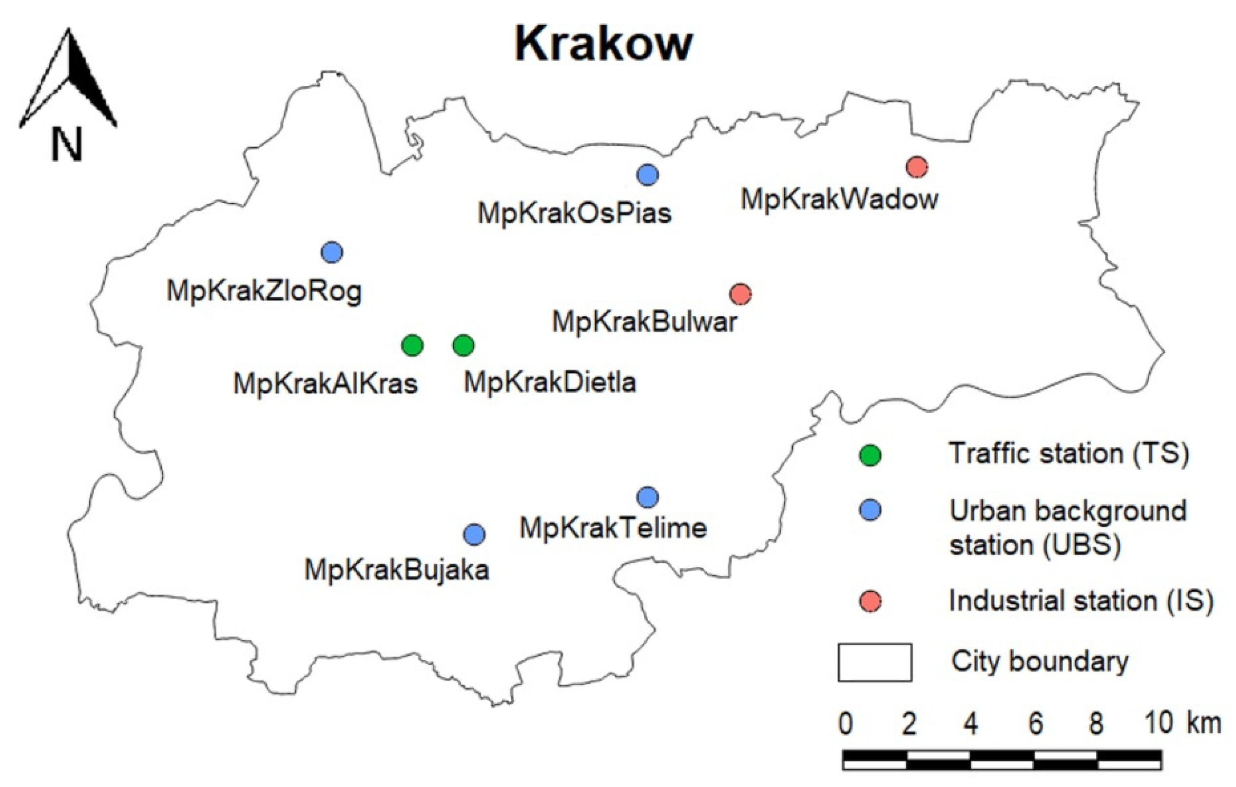
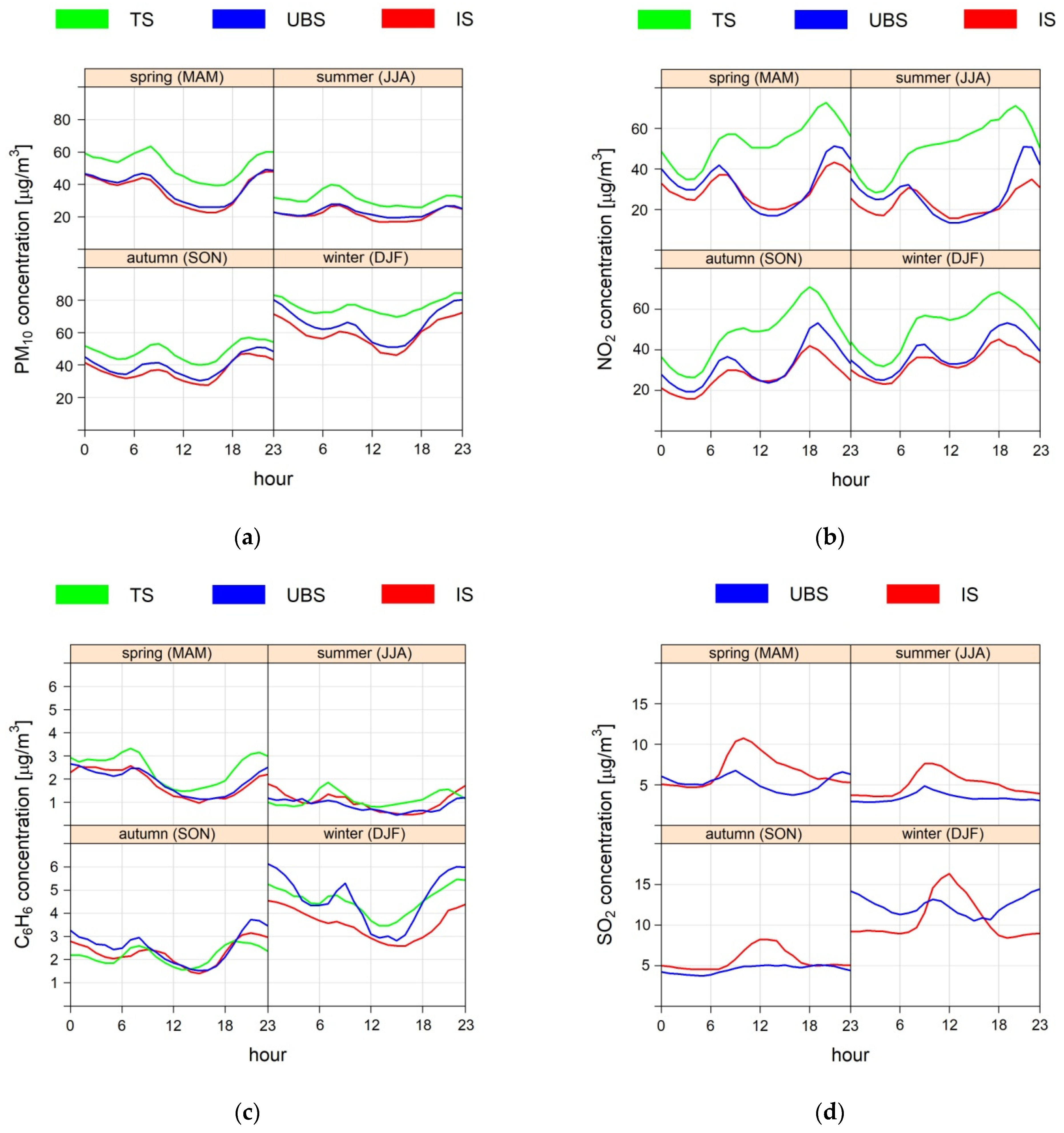
  • Traffic stations (TS): Krasinski Av. (MpKrakAlKras) and Dietla St. (MpKrakDietla), which are exposed mainly on emissions of air pollutants from road transport;
  • Urban background stations (UBS): Bujaka St. (MpKrakBujaka), Osiedle Piastow (MpKrakOsPias), Zloty Rog St. (MpKrakZloRog), Telimeny St. (MpKrakTelime), located in areas representing average for the city exposure of the inhabitants to air pollution;
  • Industrial stations (IS): Bulwarowa St. (MpKrakBulwar) and Osiedle Wadow (MpKrakWadow), situated in the area affected by emission from industrial plants in north-eastern part of the city.
The location of these stations was presented on Figure 1.
The measurements with 1-h resolution of following substances concentrations were analyzed: particulate matter PM10; nitrogen dioxide (NO2), sulfur dioxide (SO2) and benzene (C6H6). The concentrations were measured automatically (continuous measurements) with resolution of 1 h using following methods (equipment):
  • PM10–β-ray attenuation (Bam 1020 fine dust monitor/Met One Instruments, Inc.) or light scattering (Grimm EDM 180 or Fidas® 200 E fine dust monitor);
  • NO2–chemiluminescence (the model T200 NO/NO2/NOx analyzer/Teledyne API);
  • C6H6–gas chromatograph with a built-in Tenax GR pre-concentration system and PID detector (Syntech Spectras GC955 series 600 BTEX analyzer);
  • SO2–UV fluorescence (the model T100 SO2 analyzer/Teledyne API).
All the measurement methods used ensure appropriate data quality in accordance with [12] and the measuring ranges of the equipment used are adequate to the pollutant concentrations occurring in the air. The type of pollutants measured continuously in the analyzed period at individual stations is presented in Table 1.

2.2. Principles of the Methodology

In order to assess the variability of data series originating from specific type of stations, a range of statistical tools enabling to compare data series and analyze the degree of similarity between them was applied. There was an assumption that a particular type of station is characterized by time series of concentrations of each substance, averaged for all stations representing this type.
First of all, the mean values for each type of stations were calculated. This means that for every 1-h record there was calculated mean value from all stations belonging to particular type of AQM station. The obtained time series of “station type averages” (STA) for every substance were further analyzed. The calculated ratios between STA were considered as the basic measure of similarity. These data were then grouped by different time intervals (hours, months, seasons) and presented on plots.
In the purpose of better understanding the similarities and differences between the data, cluster analysis and statistical significance tests were also applied.
In summary, the assumptions of created methodology are as follows:
  • Time series of averaged concentrations for each type of AQM station (traffic, urban background, industrial) were taken into account in the analyses and called “station type averages” (STA). In the case when the concentrations of specific pollutant from only one station were available, these data were adopted and considered as the STA;
  • Urban background stations are treated as reference stations, i.e., when analyzed records from traffic or industrial stations, they were related to urban background stations.

2.3. Statistical Techniques and Visualisations

Data series of PM10, NO2, C6H6 and SO2 concentrations in the air, averaged according to the above-mentioned principles, were presented on scatter plots generated via R programming environment [104,105,106,107]. The special mode of these plots (hexagonal binning), aggregating dense groups of data points into polygons, was applied. This allowed us to not only examine relationships between variables but also to analyze the density of data points in particular part of the graph.
In order to investigate the variability of station types the concentration ratios of analyzed substances were calculated. These ratios were expressed as STA of specific pollutant on traffic/industrial stations divided by STA of the same substance on urban background stations (according to the methodology). The time series of raw data and the time series of the calculated ratios were visualized on timeVariation plots, produced in R programming environment [105] (package openair [106]). Other graphs were prepared in ggplot2 package [107], also in R.
The agglomerative hierarchical clustering was conducted in this research. As a distance measure the Euclidean distance was applied and Ward linkage was selected for the purpose of determining the proximity between clusters. Ward linkage is considered the most effective method [41]. The station types for each substance were clustered in our research and the interpretation of possibly created clusters of different substances (e.g., PM10 and C6H6) was of less interest.
In this study, two different tests were performed and compared: the dependent samples t-test and the Wilcoxon signed-rank test. Before performing tests, data distribution was examined for normality. As it was proved that the distribution of the input data is not normal, the parametric tests properly should not be used. However, the data set consists of several thousands of observations. In such case, the combination of methods was proposed: t-test, Wilcoxon test and t-test after Box–Cox transformation, which ensured the normality of distribution. The results obtained from each of the methods were compared. Significance tests and Box–Cox transformation were carried out in Statistica 13.

3. Results

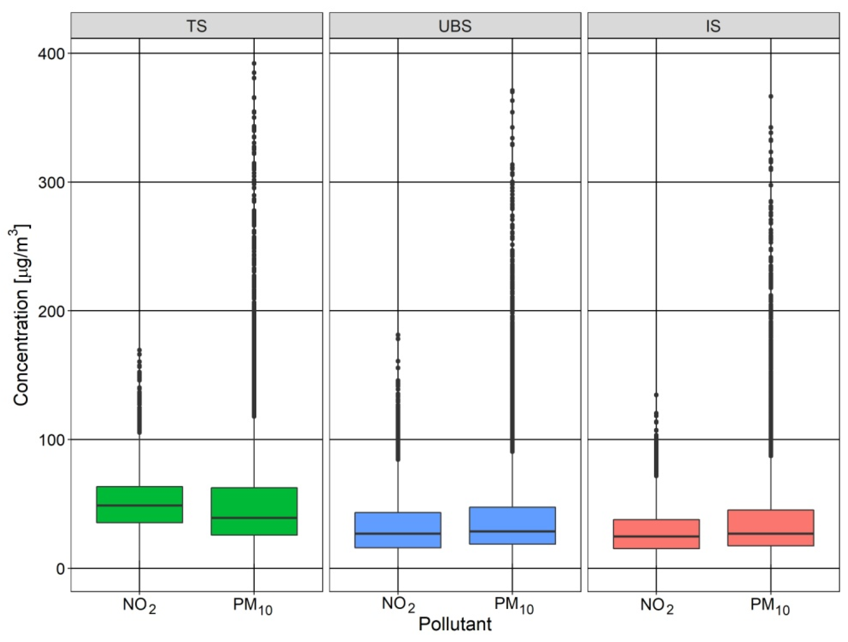
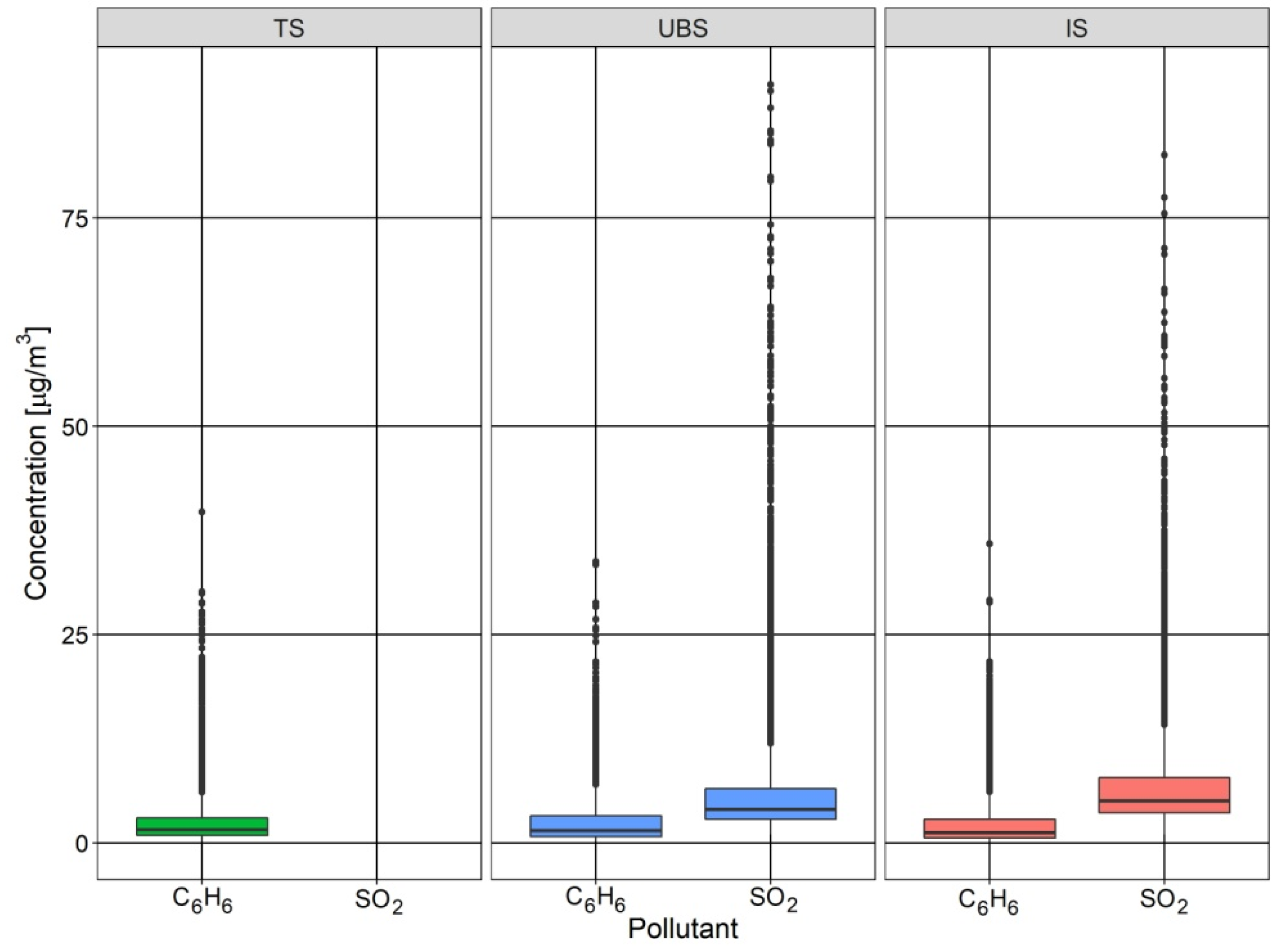
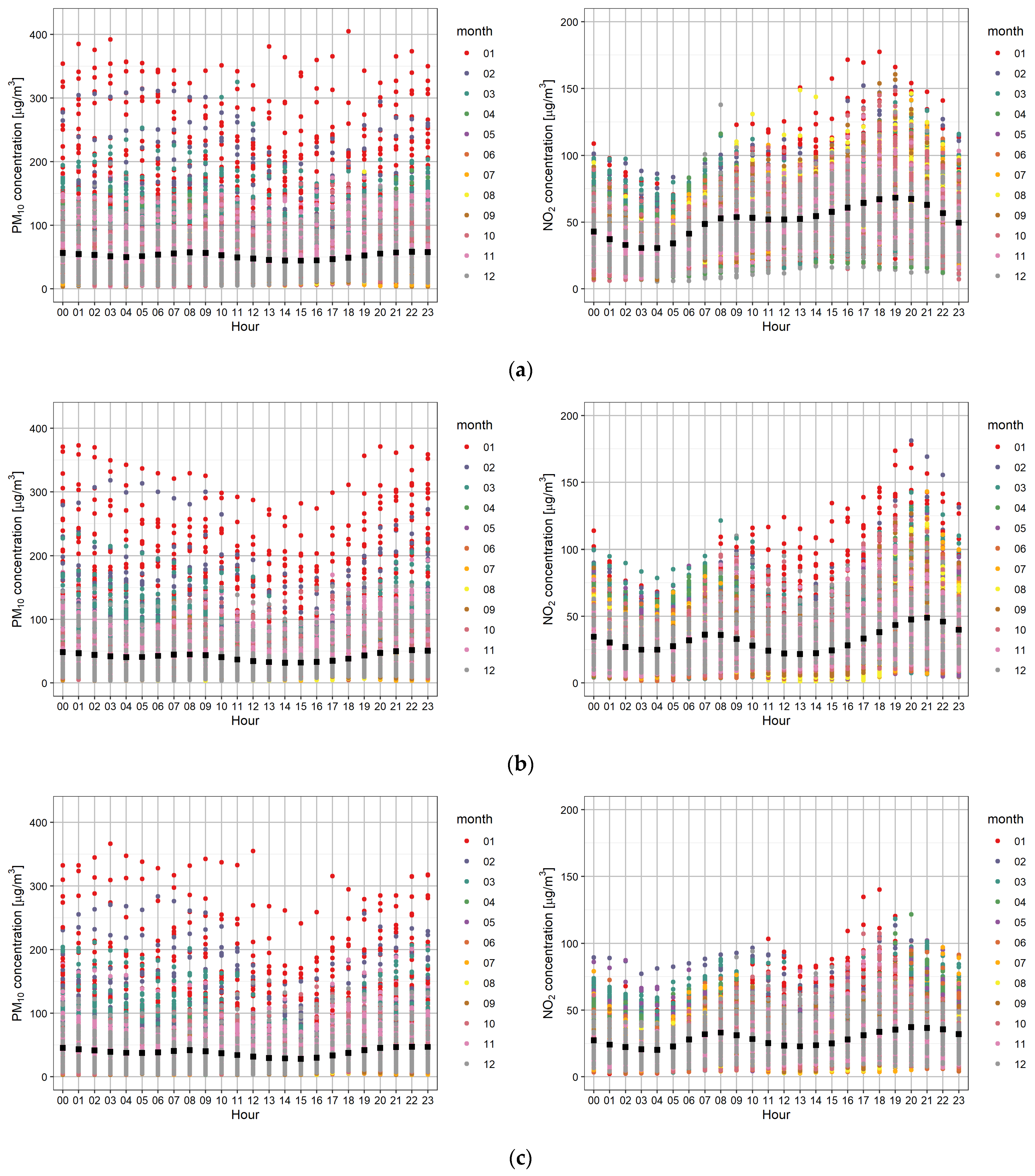
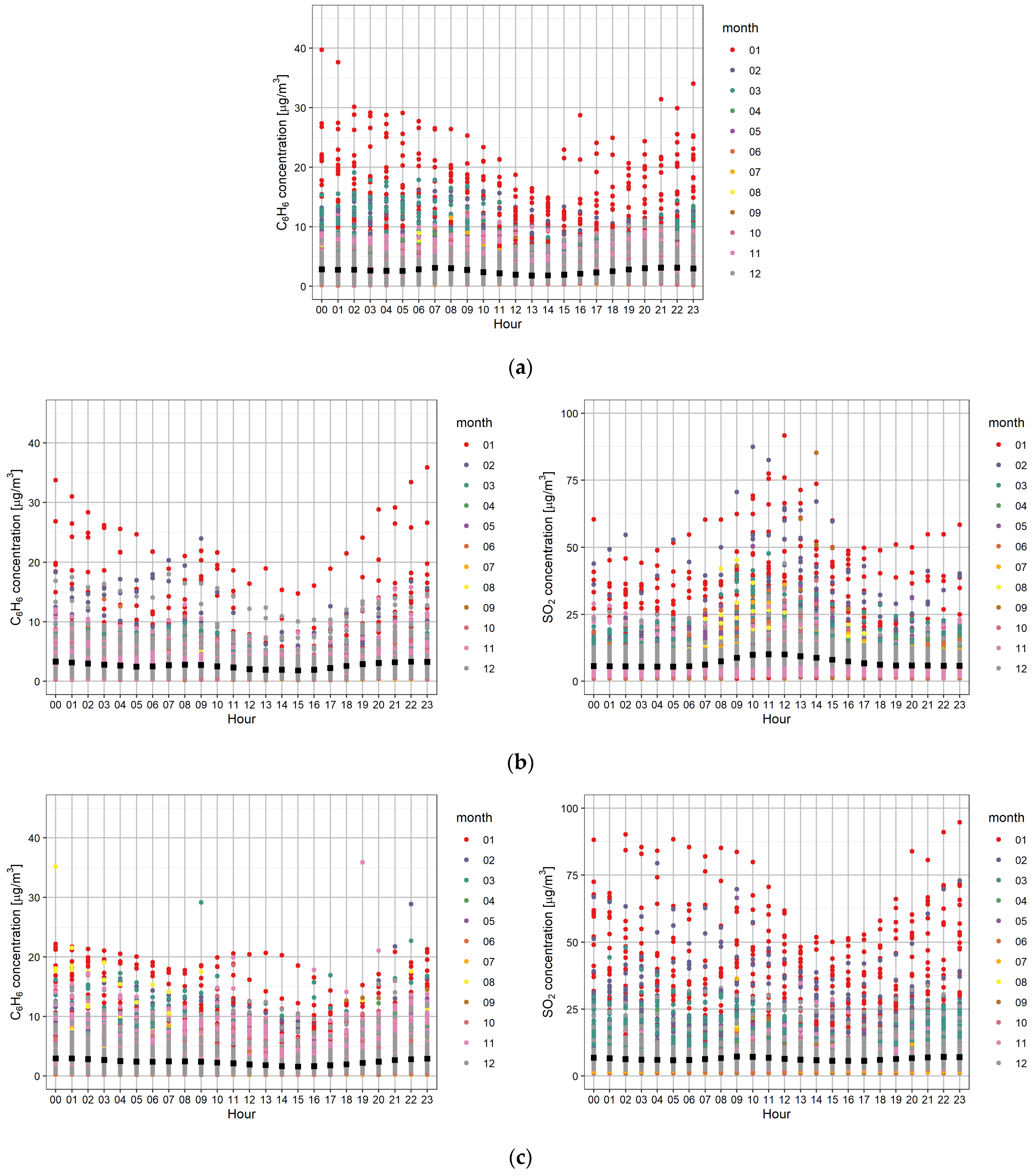
3.1. Statistical Distribution of 1-Hour Concentrations

The statistical distribution of 1-h concentrations of the analyzed pollutants in the air for individual types of air quality monitoring stations in Krakow in 2017–2018 is presented in Figure 2 and Figure 3 in the form of boxplot charts. A horizontal dash inside the box represents the median, and the border dashes of the box represent the 25% and 75% quantiles, respectively. Outliers are also shown in these figures (values greater than 150% of the interquartile range).
Traffic stations (TS) are characterized by the highest median values of NO2 and PM10 concentrations, compared to other station types, which is reflected in the boxplots (Figure 2). In the case of C6H6 and SO2 the median concentrations for individual types of monitoring stations are comparable to each other—there is no noticeable difference (Figure 3). It can be noted that there occur outlying points, which can be several times higher than the respective median value.

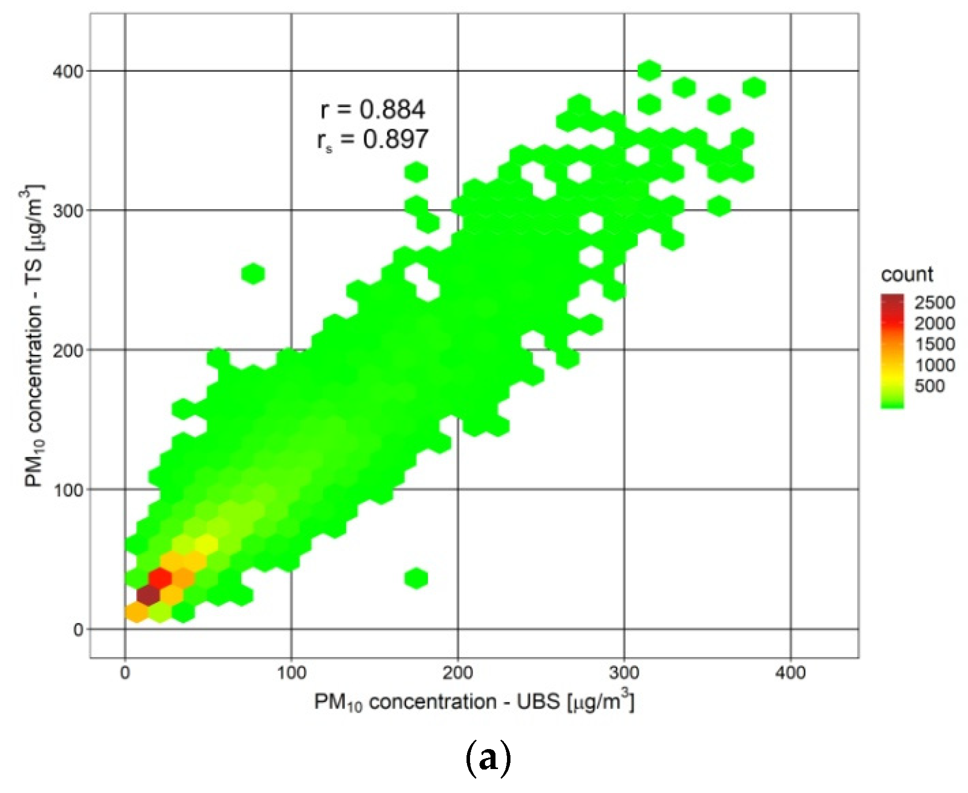
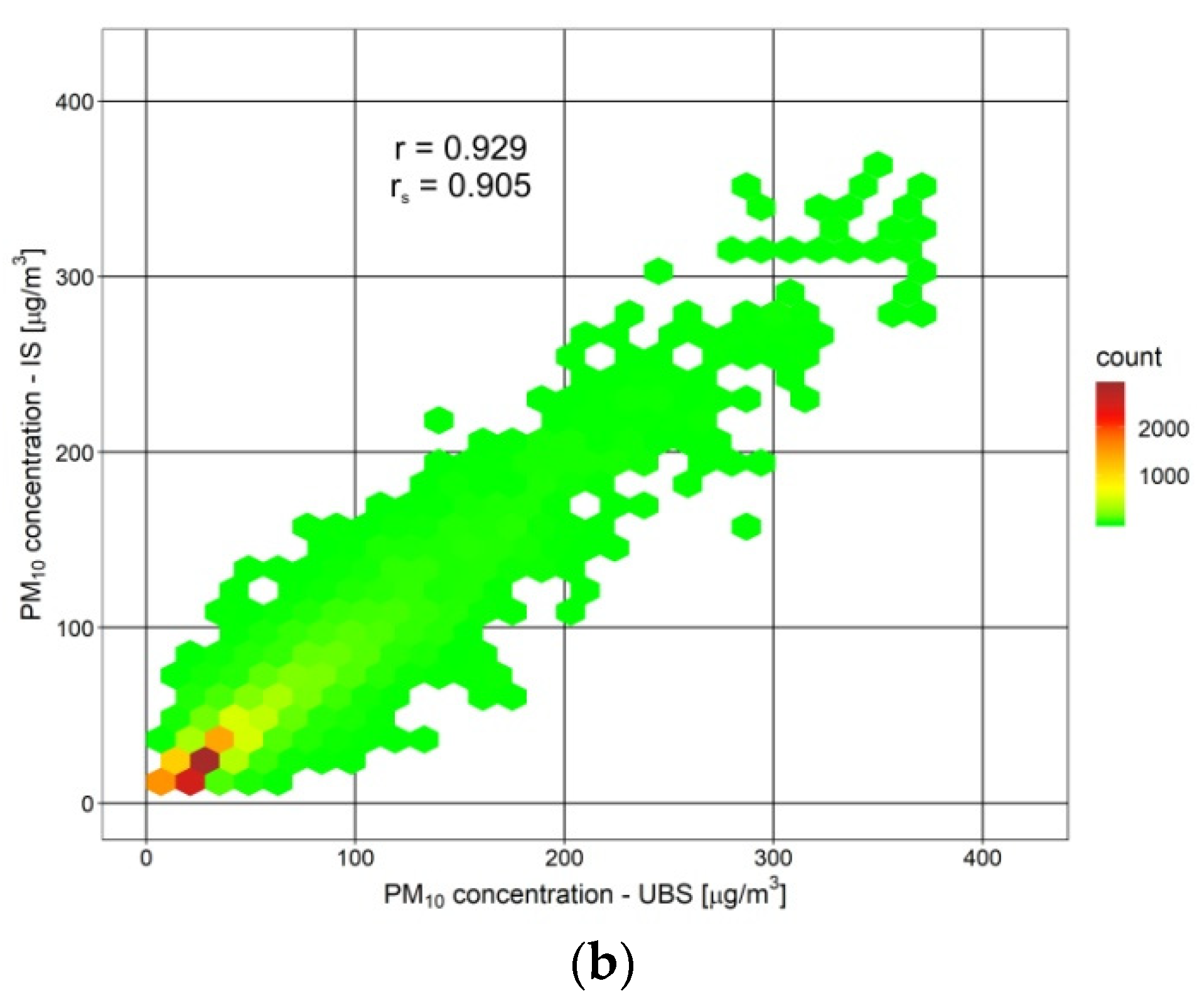
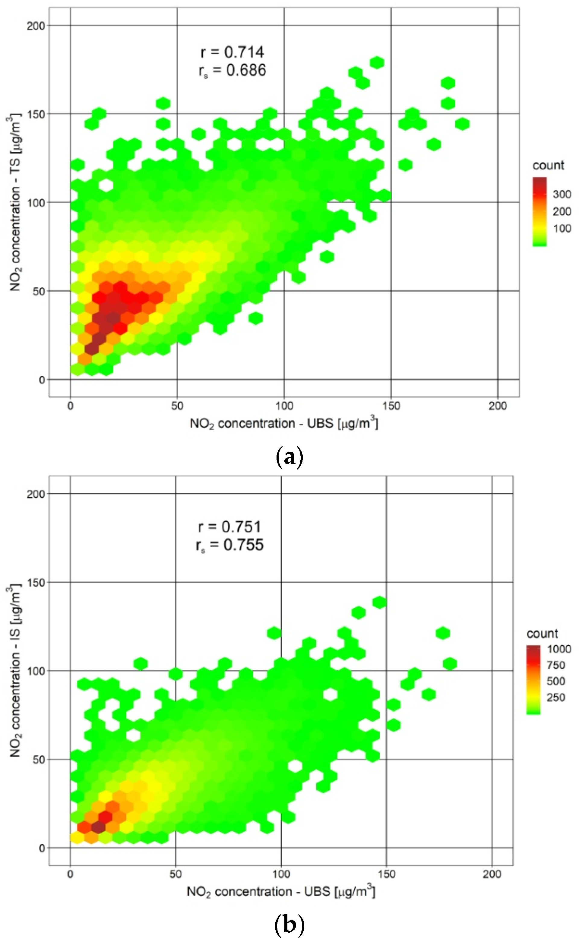
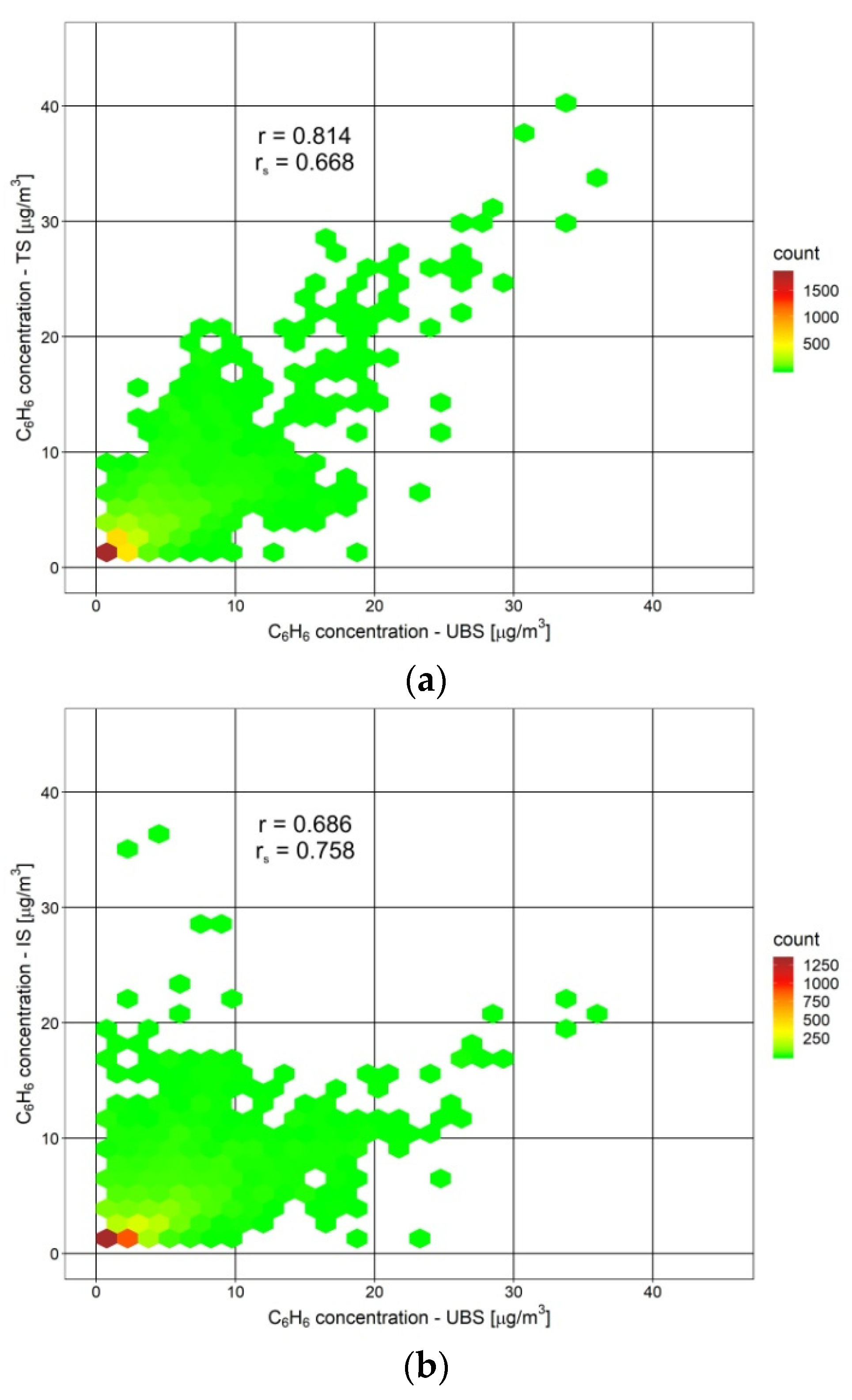
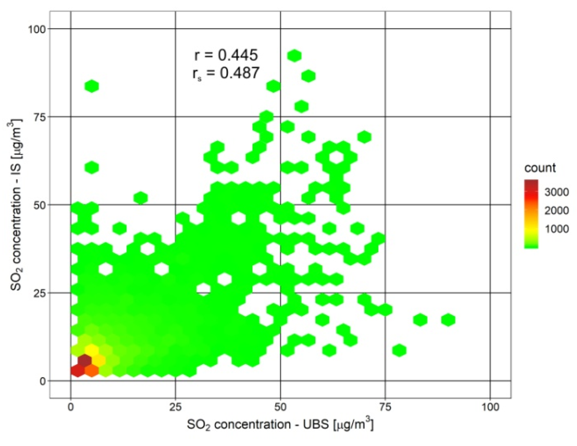
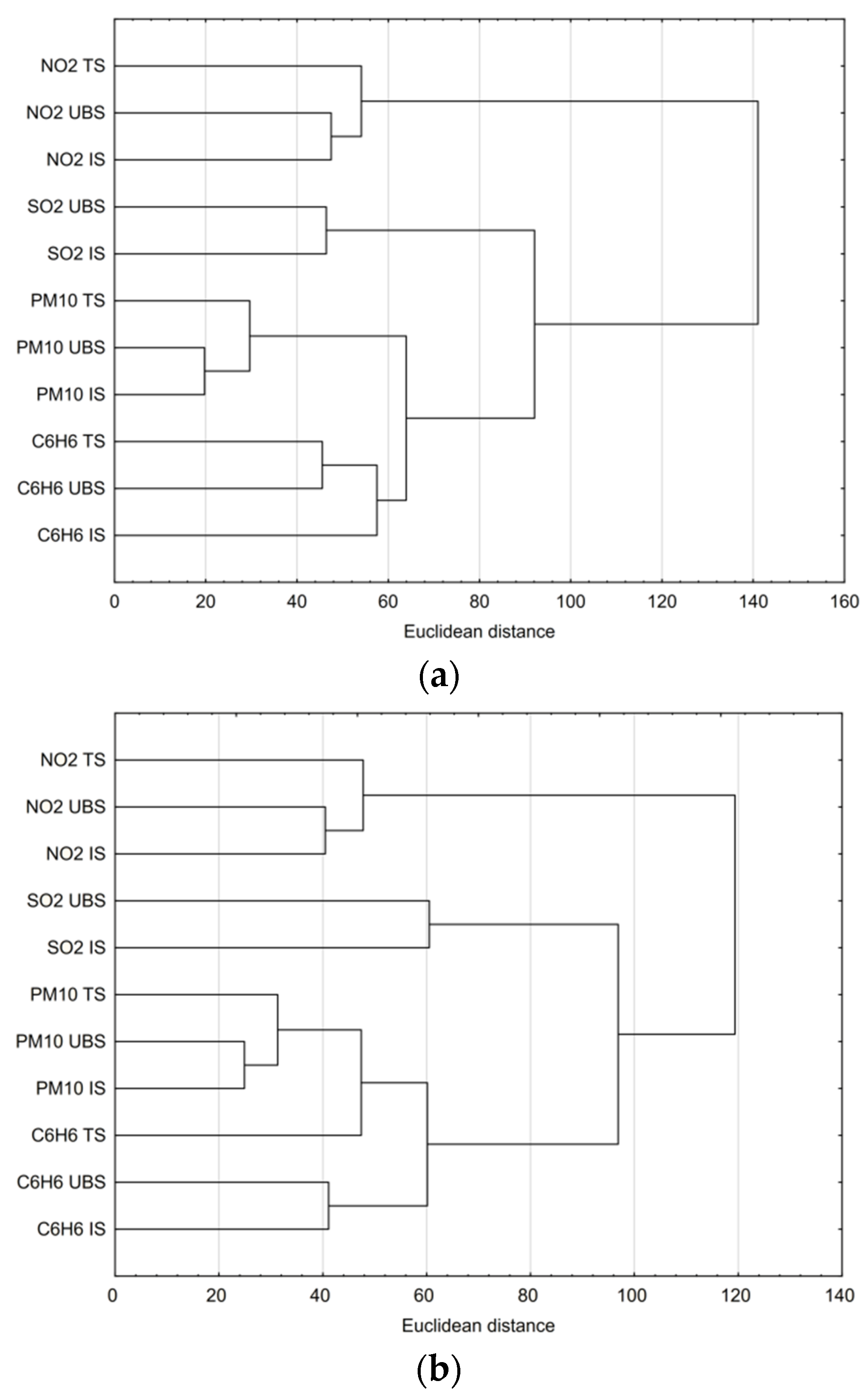
3.2. Interdependencies of 1-Hour Concentrations between AQM Station Types

There is an observed clear linearity between a certain type of station (traffic and industrial, respectively) in relation to the values measured at urban background stations (UBS) in case of PM10 concentrations (Figure 4). The highest density of observations on the scatterplots falls on the values of 100 μg/m3 or lower. In contrast to the PM10, the relationship between NO2 concentration for traffic and urban background stations is likely to be non-linear (Figure 5). There is observed a similar pattern regarding C6H6 and SO2 concentrations (Figure 6 and Figure 7). In order to better visualize the relationships between the 1-h concentrations observed at different types of AQM stations, the Pearson correlation coefficient (r) and Spearman’s rank correlation coefficient (rs) are also presented in Figure 4, Figure 5, Figure 6 and Figure 7.
The results of performed cluster analysis are presented in Figure 8 and Table 2 and Table 3. Two variants of analysis were conducted, with and without outliers, in order to assess the effect of outliers exclusion. In both cases Euclidean distance was applied as a measure of similarity. Despite the slight differences for PM10 and C6H6, the main tendency of clustering IS and UBS together and TS separately was still present. For all substances, except benzene, this tendency is present both in the example with and without outliers. In the case of C6H6 including outliers, the TS and UBS types are clustered together and IS type is separated from them.
As it results from the significance tests carried out in order to compare the mean 1-h results of measurements of pollutant concentrations observed at individual types of stations (Table 4 and Table 5), all analyzed differences were recognized as statistically significant (p < 0.05). This means that all types of stations differ from each other in terms of the concentration of each of the pollutants under consideration.
All three statistical tests gave the similar results. Transforming the original data to a normal distribution did not affect the final result of the Student’s t-test. It can be concluded that the large sample size used was sufficient to apply the parametric test.

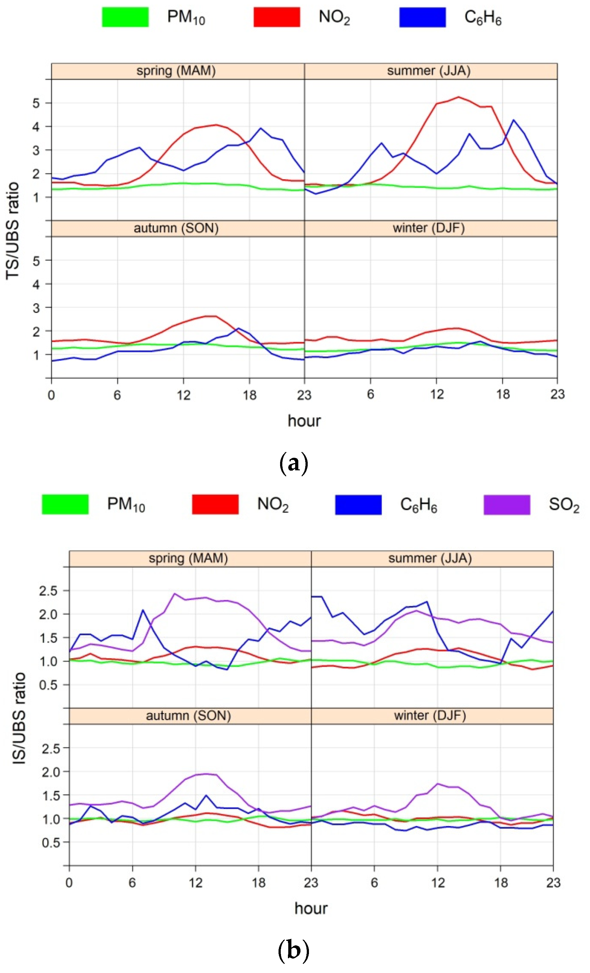
3.3. Temporal Variability of 1-Hour Concentrations and Type Station Ratios

Temporal variability of 1-h air concentrations of analyzed pollutants is shown in Figure A1 and Figure A2 (Appendix A) and Figure A3 (Appendix B). As it results from the data presented in Figure A1 the majority of points representing single 1-h concentrations of PM10, which exceed 100 μg/m3 (the information threshold for PM10 obligatory in Poland) was recorded in winter months. This suggests that maximal concentrations are more likely to occur in the middle of the heating season. The situation is similar for the other analyzed substances (Figure A1, Figure A2 and Figure A3); however, a certain exception in this case is NO2, for which the seasonal increase in air concentrations in winter months is relatively small.
The black squares in Figure A1 and Figure A2 are representing mean value grouped by hour of a day. There is observed a clear tendency of maximal and minimal values depending on the hour of a day. The maximum values among the averages calculated for a specific hour occurred in the hours 7:00–9:00 and 19:00–23:00 for the industrial station and urban background station. The discussed dependence is slightly different in the case of traffic stations. In the morning hours there is no clear maximum, while in the second half of the day the maximum falls in the time period 18:00–20:00.
The concentrations of NO2 and PM10 at traffic stations in each season of the year are clearly higher than the concentrations of these substances at urban and industrial background stations in the respective periods (Figure 9). For example, in the summer, 1-h NO2 concentrations in the afternoon at traffic stations are even five times higher than the correspondingly determined concentrations of this substance at the urban background station, while in summer this exceedance is almost twice as high. In the non-heating season (late spring and summer months) clearly increased C6H6 concentrations are also observed at the traffic and industrial stations compared to the urban background station (Figure 9a).

4. Discussion

The period of time analyzed in this study (2017–2018) reflects the air quality in Krakow in the final period of the gradual decommissioning of low-power boilers and stoves, fired with solid fuels, but before the introduction of a complete ban on their use, introduced from 1 September 2019 [48]. Previously, there were also significant reductions in air pollutant emissions (mainly SO2) from local industrial plants.
Statistical distributions of 1-h concentrations of analyzed pollutants in the air visualized using boxplots (Figure 2 and Figure 3) show that at least half of the 1-h measurement data is concentrated near the median (narrow interquartile ranges determined by the height of the boxes). Thus, the high variation in the values of 1-h concentrations during the year results mainly from the outliers that appear periodically during particularly unfavorable weather conditions with the increased impact of local and influx emission sources. Among the analyzed substances, the highest values of their concentrations in the air (also in relation to the relevant permissible levels) are observed for PM10 and NO2, and the lowest for C6H6 and SO2. Indirectly, this indicates a relatively small impact on the air quality in Krakow of local SO2 emission sources (decommissioning of low-power coal-fired furnaces and boilers, commissioning of the flue gas desulphurization installation in the municipal heat and power plant). The generally low air concentrations of SO2 previously observed at the traffic station (MpKrakAlKras) [102,103], were also the basis for resigning from the measurements of SO2 at this station a few years ago.
High correlation coefficients between PM10 concentrations for analyzed types of AQM stations (Figure 4) result from the impact of similar emission sources (PM10 might originate from same sources in the analyzed period). On the other hand, the lack of a strong correlation between the series of data observed at individual types of monitoring stations observed in the case of other analyzed substances (NO2, C6H6 and SO2) (Figure 5, Figure 6 and Figure 7) confirms their significant differentiation in terms of the dominant emission sources. Thus, it indicates their proper location enabling the implementation of the main measurement objectives assigned to a given type of station. There is a weaker correlation in the case of pair TS/UBS than IS/UBS, which confirms the impact of traffic emission on the dissimilarity of these two data series. It may suggest that traffic emission from busier and more congested roads has a more pronounced impact on the measurement results than a combination of other pollution sources, including industrial emission sources.
Slightly more detailed dependencies in this respect result from the cluster analysis. Cluster analysis is a technique allowing to create groups (clusters) of data (objects, statistical observations), when there is not known any “natural” set of classes for these data. The objects belonging to particular cluster are as similar as possible to each other in this cluster and as different as possible according to objects from another clusters. Therefore, it is possible to discover some unobvious information in input data, recognize patterns hidden for “classical” statistical methods, define the level of similarity between the data features and organize data into groups, which are easy to explain and interpret. The obtained results of the cluster analysis show much smaller similarities between traffic stations and other types of stations. It can be clearly explained by higher concentrations of examined substances (especially NO2 and PM10) recorded at traffic stations, stemming from the stronger impact of traffic emission and poorer ventilation conditions in street canyons compared to the other sites. The analysis of the distance matrix (Table 2 and Table 3) shows that traffic and industrial stations are the least similar to each other, and the industrial and urban background stations are the most similar. The latter regularity indicates the possibility of overlapping, under certain conditions, the impact of the urban background on the results of measurements at industrial stations, which was demonstrated for Krakow in [24]. From the main tendency of clustering IS and UBS together and TS separately (Figure 8) it can be concluded that the traffic stations located in the center of Krakow within the second ring road fulfill their role. They record the impact on the air quality of local and transit road transport related to routes with high car traffic intensity with periodically forming traffic jams. On the other hand, industrial sources have a minimal effect on the level of pollutant concentrations measured at these stations.
Statistical significance tests are intended, among others, for verification if observed differences between statistics calculated from compared samples (e.g., mean, median) are coincidental (insignificant) or they result from a certain effect and therefore they are not coincidental (significant). Some of the significance tests are applied in situations when there are compared two samples representing various conditions of measurements. This means that all types of stations differ from each other in terms of the concentration of each of the pollutants under consideration. The conducted statistical tests (Table 4 and Table 5) show that air concentrations of analyzed pollutants at individual types of AQM stations differ significantly from each other. This may indicate the impact of different groups of pollution sources on considered stations. This conclusion is confirmed by the results of the cluster analysis, especially in relation to traffic stations that were in a separate cluster from the urban background and industrial stations (Figure 8).
In the case of PM10, NO2 and C6H6 the highest concentration values are observed at traffic stations and the lowest at urban and industrial background stations, while the concentrations of PM10 and C6H6 are definitely higher in the heating season than in the non-heating season, and NO2 concentrations are usually not subject to large seasonal fluctuations, as they are mainly shaped by road transport (Figure A1, Figure A2, Figure A3 and Figure 9). Increased concentration values at traffic stations are most evident in the case of NO2. On this basis, it can be concluded that this type of stations differs most from the others in terms of NO2 concentration, which, among the pollutants analyzed in the study, seems to be the most typical pollution for road transport. No significant differences between the winter and summer months or the transition period for NO2 concentrations in the air at traffic stations is confirmed by the results obtained in previous studies [22,61,75]. Strong seasonal variations of the air concentrations observed for the rest of analyzed substances can be explained, on the one hand, by higher emissions (municipal and household sector), and on the other hand, it results from weaker ventilation and a lower mixing-layer height, which was already demonstrated for previous years, e.g., in the works [58,60,64]. There is also a clear seasonal trend in the case of SO2 concentrations, but this is reflected in the periodic impact of industrial plants (combined heat and power plant and steel mill) on the measurement results, recorded especially at an industrial station located within the range of the impact of these emission sources [24,75].
Poor air quality in Krakow, often observed during the heating season, is usually associated with unfavorable synoptic-scale (anti-cyclonic circulation), low temperature, low mixing-layer height and low wind speed, which hinders the dispersion of pollutants in the air [58,60,61,64,65], and in the case of fine solid particles with increased formation of secondary inorganic (SIA) or organic (SOA) aerosols [62,68,69,70,71] and a large inflow background of dust pollution from adjacent areas [22,24,65,67]. Despite a significant reduction of SIA precursor emissions from large combustion plants (SO2 and NOx) and residential heating (SO2), the contribution of SIA formation in fine particulate matter is now much greater [68,69,70] than it has been reported for several years ago [72,73]; this indicates an increase in the role of NOx (derived from combustion processes, including to a large extent from the combustion of engine fuels) in the formation of SIA, and thus their greater impact on the levels of fine particulate matter in the air [91,92,97].
Increased C6H6 concentrations in the non-heating season at the traffic station (MpKrakAlKras) compared to the urban background station (MpKrakBujaka) (Figure 9a) indicate that the main source of C6H6 in this season is emission from road transport, which is also confirmed, among others, by in the results of earlier measurements carried out in Krakow in the summer at several points in the immediate vicinity of a busy street and petrol station [108] and also in other cities in various locations [109,110,111]. Benzene concentrations measured at the industrial station (MpKrakBulwar) in the non-heating season are also significantly higher than those measured at the urban background station (Figure 9b), which results from the relatively close location of the MpKrakBulwar station to the fuel station (approximately 60 m) and a large junction (approximately 100 m), as well as within the range of the periodic impact of a coking plant (operating as part of a steelworks) located approximately 3–4 km from this monitoring station [24]. This corresponds to the research results presented by Notario et al. [111]. A clear increase in C6H6 concentrations in the vicinity of petrol stations was also demonstrated, among others, by Bogacki et al. [108] and Karakitsios et al. [112]. As it results from the work [24] at the MpKrakBulwar industrial station, depending on the wind direction, the impact of emissions not only from the nearby steel plant, but also from other nearby industrial plants (including heat and power plant and municipal waste incineration plant) is also recorded, which is reflected, i.a., in a clear periodic increase in SO2 and NO2 concentrations in relation to the urban background station located far from these plants (Figure 9b).
In the case of PM10 concentrations at all AQM stations, including traffic stations, very similar daily trends are observed (Figure A3). This indicates that the level of these concentrations in the whole of Krakow is greatly influenced by meteorological factors characterized by daily variability (including, in particular, the wind speed and the mixing-layer height [60,64]) and the dominant influence of emission sources and phenomena occurring to a large extent across the city (urban, suburban and regional background and local formation of secondary aerosols from gaseous pollutants [67,68,71,73,75]). On the other hand, the observed daily variability of the NO2 and C6H6 concentration ratios at TS and UBS monitoring stations (Figure 9b) in the summer and spring months reflects the mechanisms of NO2 formation occurring during the day (oxidation of NO from engine emissions, e.g., with ozone and hydroxyl or hydrocarbon radicals), as well as the atmospheric destruction of benzene or its photo-oxidation towards the formation of SOA [113,114,115].
The diurnal variation of air pollutants is strongly controlled not only by temporal variation of emission levels and photochemical reactions but also by vertical turbulent mixing related to the vertical temperature gradient and the mixing-layer height. The sudden increase of vertical mixing in the morning leads to the drop of pollutant concentrations in the air. The strong mixing during the daytime also keeps low concentrations. In the late afternoon mixing becomes weak and concentrations start to increase. This so-called rectifier effect [116,117] can be seen in Figure A3, except for NO2 at TS stations (due to strong temporal variation of emission sources and photochemical reactions). The rectifier effect can be employed to explain that the drop of concentration occurs later in the morning in winter than in summer as shown in Figure A3a,b (for UBS and IS) and Figure A3c. The different magnitudes of PM10, C6H6 and SO2 between summer and winter are due to different vertical mixing in the two seasons [60,64].

5. Conclusions

The automatic air quality monitoring system in Krakow focuses mainly on the observation of the spatial and temporal variability of the concentrations of particulate matter PM10 at four urban background stations (UBS) and two industrial stations (IS) and the registration of road transport impact in this regard at two traffic stations (TS) including one station located in a deep street canyon with very heavy traffic. Additional substances measured at some stations (i.a. NO2, SO2 and C6H6) allow for the observation of additional impacts of emission sources characteristic for these substances (emissions from engine vehicles, domestic stoves, power boilers, petrol stations or a coking plant).
As shown by the analysis of measurement data available for 2017–2018, in Krakow, there is a pronounced impact of emissions from road transport on NO2 concentrations at traffic stations located in the city center within streets with high traffic and from industrial plants on SO2 concentrations recorded at the industrial station located in the north-eastern part of the city within the influence of the heat and power plant and steelworks. The influence of benzene on the results recorded at the traffic station is also noticeable, especially in the spring and summer seasons, when other emission sources of this substance functioning only during the heating season do not interfere with traffic emissions.
In the cold months associated with the heating season, the variability of the concentration ratios recorded at IS/UBS and TS/UBS stations for all analyzed pollutants is flattened, which results from the overlapping of the impact of many different emission sources in this period, and above all from the growing importance of the urban, suburban and regional background of this pollution.
Traffic stations differ from urban background and industrial stations. The last two types are more similar to each other. This was demonstrated by cluster analysis. This trend is confirmed by hourly averaged concentrations of PM10 and NO2.
In the case of various types of AQM stations, for which no very strong linear correlation is observed for the measurement results recorded on them, one can conclude about different emission sources affecting individual types of stations and areas for which they are representative. When a strong linear correlation occurs, it can be suspected that the concentrations at the stations analyzed are influenced by the same emission sources at the same time. This issue would require further research using receptor models or at least analysis of the wind speed field and direction.
The highest concentration values observed during the year usually occur in the winter months. The clear diurnal and seasonal variation in PM10 and NO2 concentrations may be due to both the variable activity of emission sources and the natural mechanisms occurring in the atmosphere, the actions of which result, for example, in the variability of vertical turbulent mixing (the height of the mixing-layer) during the daytime and depending on the season and type of atmospheric circulation. In addition, the levels of PM10 in the air are increasingly influenced by the formation of secondary inorganic and organic aerosols.
The ratio of NO2 concentrations observed at TS/UBS stations is several times higher than the one in spring and summer (when there is no significant impact of NOx emission sources other than engine emissions), which indicates that the measurement of NO2 concentration at traffic stations in Krakow is a good proxy parameter describing the impact of road transport on air quality. This substance can also be used as an indicator in the analysis of the effects of the changes introduced in the field of car traffic management and the effects of reducing vehicle traffic in connection with the COVID-19 pandemic or other large-scale incidents.
The concentrations of the remaining analyzed substances (PM10, C6H6 and SO2) are strongly dependent on the season (they significantly increase in the heating season), therefore their usefulness in air quality management should be focused mainly on the analysis of changes in emissions from the municipal and household sector (residential heating) and the industrial plants in the case of significant modernization or production stop. In the non-heating season, it is possible to identify individual impacts of other specific emission sources (road dust resuspension, fugitive particulate matter emissions from road repairs or construction works, benzene emissions from petrol stations or cooking plant, SO2 emissions from the large industrial plants, etc.). The reduction of NO2 concentrations in the air due to the commissioning of new flue gas denitrification (DeNOx) installations should also be observed within the range of impact of emissions from combined heat and power plants.
Further, more detailed analysis of monitoring data on concentrations of gaseous and particulate substances with the use of statistical tools for receptor modeling (e.g., PCA, PMF) is recommended in order to identify the main groups of sources affecting AQM stations belonging to particular types in order to better identify them and apply in activities in the field of the air quality improvement and the health risk reduction. There is a need for further research in this field, including works related to the better identification of factors influencing the air pollution in Krakow and the interdependencies between the measurement data observed at monitoring stations of various types, as well as the assessment of the effects of corrective actions taken so far and their further development. In more detailed analyses of trends in air quality changes, it is recommended to take into account the available meteorological data or to perform meteorological normalization of pollutant concentrations.

Author Contributions

Conceptualization, R.O. and T.G.; methodology, R.O. and T.G.; software, T.G.; validation, R.O. and T.G.; formal analysis, R.O. and T.G.; investigation, R.O. and T.G.; resources, R.O. and T.G.; data curation, T.G.; writing—original draft preparation, R.O. and T.G.; writing—review and editing, R.O.; visualization, T.G.; supervision, R.O.; project administration, R.O.; funding acquisition, R.O. All authors have read and agreed to the published version of the manuscript.

Funding

The paper has been prepared as part of the research connected with the subsidy of Ministry of Education and Science in Poland to maintain scientific potential (agreement no. 16.16.150.545).

Acknowledgments

The authors would like to express their sincere gratitude to the Chief Inspectorate for Environmental Protection and the Voivodeship Inspectorate of Environmental Protection in Krakow for sharing air quality monitoring data and description of the air quality monitoring system.

Conflicts of Interest

The authors declare no conflict of interest. The funders had no role in the design of the study; in the collection, analyses, or interpretation of data; in the writing of the manuscript, or in the decision to publish the results.

Appendix A

Figure A1. Distribution of average 1-h PM10 (left) and NO2 (right) concentrations at individual hours and months in Krakow in 2017–2018: (a) Traffic stations; (b) Urban background stations; (c) Industrial stations. The black squares are representing mean value grouped by hour of a day.
Sustainability 13 05623 g0a1
Figure A2. Distribution of average 1-h C6H6 (left) and SO2 (right) concentrations at individual hours and months in Krakow in 2017–2018: (a) Traffic stations; (b) Urban background stations; (c) Industrial stations. The black squares are representing mean value grouped by hour of a day.
Sustainability 13 05623 g0a2

Appendix B

Figure A3. Average air pollutant concentrations at particular types of AQM stations in Krakow calculated for hourly mean during each season (trimesters) of the years 2017–2018: (a) PM10; (b) NO2; (c) C6H6; (d) SO2. Spring: March, April and May; summer: June, July and August; autumn: September, October and November; winter: December, January and February.
Sustainability 13 05623 g0a3

References

  1. De Visscher, A. Air Dispersion Modeling: Foundations and Applications; John Wiley & Sons: Hoboken, NJ, USA, 2013. [Google Scholar]
  2. Leelőssy, Á.; Molnár, F.; Izsák, F.; Havasi, Á.; Lagzi, I.; Mészáros, R. Dispersion modeling of air pollutants in the atmosphere: A review. Cent. Eur. J. Geosci. 2014, 6, 257–278. [Google Scholar] [CrossRef]
  3. Thunis, P.; Miranda, A.; Baldasano, J.M.; Blond, N.; Douros, J.; Graff, A.; Janssen, S.; Juda-Rezler, K.; Karvosenoja, N.; Maffeis, G.; et al. Overview of current regional and local scale air quality modelling practices: Assessment and planning tools in the EU. Environ. Sci. Policy 2016, 65, 13–21. [Google Scholar] [CrossRef]
  4. Pielke, R.A.; Uliasz, M. Use of meteorological models as input to regional and mesoscale air quality models—limitations and strengths. Atmos. Environ. 1998, 32, 1455–1466. [Google Scholar] [CrossRef]
  5. Juda-Rezler, K. New challenges in air quality and climate modeling. Arch. Environ. Prot. 2010, 36, 3–28. [Google Scholar]
  6. Gulia, S.; Nagendra, S.S.; Khare, M.; Khanna, I. Urban air quality management-A review. Atmos. Pollut. Res. 2015, 6, 286–304. [Google Scholar] [CrossRef] [Green Version]
  7. Hopke, P.K. Recent developments in receptor modeling. J. Chemometr. 2003, 17, 255–265. [Google Scholar] [CrossRef]
  8. Miskell, G.; Salmond, J.; Longley, I.; Dirks, K.N. A novel approach in quantifying the effect of urban design features on local-scale air pollution in central urban areas. Environ. Sci. Technol. 2015, 49, 9004–9011. [Google Scholar] [CrossRef] [PubMed]
  9. Rybarczyk, Y.; Zalakeviciute, R. Machine learning approaches for outdoor air quality modelling: A systematic review. Appl. Sci. 2018, 8, 2570. [Google Scholar] [CrossRef] [Green Version]
  10. Masih, A. Machine learning algorithms in air quality modeling. GJESM 2019, 5, 515–534. [Google Scholar] [CrossRef]
  11. Cai, J.; Ge, Y.; Li, H.; Yang, C.; Liu, C.; Meng, X.; Wang, W.; Niu, C.; Kan, L.; Schikowski, T.; et al. Application of land use regression to assess exposure and identify potential sources in PM2.5, BC, NO2 concentrations. Atmos. Environ. 2020, 223, 117267. [Google Scholar] [CrossRef]
  12. Directive 2008/50/EC of the European Parliament and of the Council of 21 May 2008 on Ambient Air Quality and Cleaner Air for Europe. OJ L 152. 11 June 2008. Available online: https://eur-lex.europa.eu/LexUriServ/LexUriServ.do?uri=OJ:L:2008:152:0001:0044:en:PDF (accessed on 17 May 2021).
  13. Chan, C.C.; Hwang, J.S. Site representativeness of urban air monitoring stations. J. Air Waste Manag. Assoc. 1996, 46, 755–760. [Google Scholar] [CrossRef]
  14. Righini, G.; Cappelletti, A.; Cionni, I.; Ciucci, A.; Cremona, G.; Piersanti, A.; Vitali, L.; Ciancarella, L. Methodologies for the evaluation of spatial representativeness of air quality monitoring stations in Italy. EAI 2013, 1–2, 60–68. [Google Scholar]
  15. Miñarro, M.D.; Bañón, D.; Egea, J.A.; Costa-Gómez, I.; Caracena, A.B. A multi-pollutant methodology to locate a single air quality monitoring station in small and medium-size urban areas. Environ. Pollut. 2020, 266, 115279. [Google Scholar] [CrossRef] [PubMed]
  16. Li, F.; Zhou, T.; Lan, F. Relationships between urban form and air quality at different spatial scales: A case study from northern China. Ecol. Indic. 2021, 121, 107029. [Google Scholar] [CrossRef]
  17. Cyrys, J.; Eeftens, M.; Heinrich, J.; Ampe, C.; Armengaud, A.; Beelen, R.; Bellander, T.; Beregszaszi, T.; Birk, M.; Cesaroni, G.; et al. Variation of NO2 and NOx concentrations between and within 36 European study areas: Results from the ESCAPE study. Atmos. Environ. 2012, 62, 374–390. [Google Scholar] [CrossRef]
  18. Guerreiro, C.B.; Foltescu, V.; De Leeuw, F. Air quality status and trends in Europe. Atmos. Environ. 2014, 98, 376–384. [Google Scholar] [CrossRef] [Green Version]
  19. Schiavon, M.; Redivo, M.; Antonacci, G.; Rada, E.C.; Ragazzi, M.; Zardi, D.; Giovannini, L. Assessing the air quality impact of nitrogen oxides and benzene from road traffic and domestic heating and the associated cancer risk in an urban area of Verona (Italy). Atmos. Environ. 2015, 120, 234–243. [Google Scholar] [CrossRef]
  20. Ortolani, C.; Vitale, M. The importance of local scale for assessing, monitoring and predicting of air quality in urban areas. Sustain. Cities Soc. 2016, 26, 150–160. [Google Scholar] [CrossRef]
  21. Chlebowska-Styś, A.; Sówka, I.; Kobus, D.; Pachurka, Ł. Analysis of concentrations trends and origins of PM10 in selected European cities. E3S Web Conf. 2017, 17, 00013. [Google Scholar] [CrossRef] [Green Version]
  22. Oleniacz, R.; Gorzelnik, T.; Szulecka, A. A comparative analysis of air pollutant concentrations and inflow trajectories: A case study of selected cities in South-Eastern Poland. E3S Web Conf. 2018, 45, 00060. [Google Scholar] [CrossRef]
  23. Paraschiv, S.; Paraschiv, L.S. Analysis of traffic and industrial source contributions to ambient air pollution with nitrogen dioxide in two urban areas in Romania. Energy Procedia 2019, 157, 1553–1560. [Google Scholar] [CrossRef]
  24. Oleniacz, R.; Gorzelnik, T.; Bogacki, M. Impact of urban, suburban and industrial background on air pollution levels of dust substances in North-Eastern part of Krakow (Poland). IOP Conf. Ser. Earth Environ. Sci. 2021, 642, 012013. [Google Scholar] [CrossRef]
  25. Kim, E.; Hopke, P.K.; Pinto, J.P.; Wilson, W.E. Spatial variability of fine particle mass, components, and source contributions during the regional air pollution study in St. Louis. Environ. Sci. Technol. 2005, 39, 4172–4179. [Google Scholar] [CrossRef] [PubMed]
  26. Vardoulakis, S.; Gonzalez-Flesca, N.; Fisher, B.E.; Pericleous, K. Spatial variability of air pollution in the vicinity of a permanent monitoring station in central Paris. Atmos. Environ. 2005, 39, 2725–2736. [Google Scholar] [CrossRef]
  27. Nguyen, H.T.; Kim, K.H. Evaluation of SO2 pollution levels between four different types of air quality monitoring stations. Atmos. Environ. 2006, 40, 7066–7081. [Google Scholar] [CrossRef]
  28. Azmi, S.Z.; Latif, M.T.; Ismail, A.S.; Juneng, L.; Jemain, A. Trend and status of air quality at three different monitoring stations in the Klang Valley, Malaysia. Air Qual. Atmos. Health 2010, 3, 53–64. [Google Scholar] [CrossRef] [Green Version]
  29. Henne, S.; Brunner, D.; Folini, D.; Solberg, S.; Klausen, J.; Buchmann, B. Assessment of parameters describing representativeness of air quality in-situ measurement sites. Atmos. Chem. Phys. 2010, 10, 3561–3581. [Google Scholar] [CrossRef] [Green Version]
  30. Joly, M.; Peuch, V.H. Objective classification of air quality monitoring sites over Europe. Atmos. Environ. 2012, 47, 111–123. [Google Scholar] [CrossRef]
  31. Mavroidis, I.; Ilia, M. Trends of NOx, NO2 and O3 concentrations at three different types of air quality monitoring stations in Athens, Greece. Atmos. Environ. 2012, 63, 135–147. [Google Scholar] [CrossRef]
  32. Krynicka, J.; Drzeniecka-Osiadacz, A. Analysis of Variability in PM10 Concentration in the Wrocław Agglomeration. Pol. J. Environ. Stud. 2013, 22, 1091–1099. [Google Scholar]
  33. Barrero, M.A.; Orza, J.A.G.; Cabello, M.; Cantón, L. Categorisation of air quality monitoring stations by evaluation of PM10 variability. Sci. Total Environ. 2015, 524–525, 225–236. [Google Scholar] [CrossRef] [PubMed]
  34. Piersanti, A.; Vitali, L.; Righini, G.; Cremona, G.; Ciancarella, L. Spatial representativeness of air quality monitoring stations: A grid model based approach. Atmos. Pollut. Res. 2015, 6, 953–960. [Google Scholar] [CrossRef]
  35. Zhao, L.; Xie, Y.; Wang, J.; Xu, X. A performance assessment and adjustment program for air quality monitoring networks in Shanghai. Atmos. Environ. 2015, 122, 382–392. [Google Scholar] [CrossRef]
  36. Li, T.; Zhou, X.C.; Ikhumhen, H.O.; Difei, A. Research on the optimization of air quality monitoring station layout based on spatial grid statistical analysis method. Environ. Technol. 2018, 39, 1271–1283. [Google Scholar] [CrossRef]
  37. Wang, C.; Zhao, L.; Sun, W.; Xue, J.; Xie, Y. Identifying redundant monitoring stations in an air quality monitoring network. Atmos. Environ. 2018, 190, 256–268. [Google Scholar] [CrossRef]
  38. Alfoldy, B.; Mahfouz, M.M.K.; Yigiterhan, O.; Safi, M.A.; Elnaiem, A.E.; Giamberini, S. BTEX, nitrogen oxides, ammonia and ozone concentrations at traffic influenced and background urban sites in an arid environment. Atmos. Pollut. Res. 2019, 10, 445–454. [Google Scholar] [CrossRef]
  39. Munir, S.; Mayfield, M.; Coca, D.; Jubb, S.A. Structuring an integrated air quality monitoring network in large urban areas–Discussing the purpose, criteria and deployment strategy. Atmos. Environ. X 2019, 2, 100027. [Google Scholar] [CrossRef]
  40. Sówka, I.; Chlebowska-Styś, A.; Pachurka, Ł.; Rogula-Kozłowska, W.; Mathews, B. Analysis of particulate matter concentration variability and origin in selected urban areas in Poland. Sustainability 2019, 11, 5735. [Google Scholar] [CrossRef] [Green Version]
  41. Govender, P.; Sivakumar, V. Application of k-means and hierarchical clustering techniques for analysis of air pollution: A review (1980–2019). Atmos. Pollut. Res. 2020, 11, 40–56. [Google Scholar] [CrossRef]
  42. He, H.-D.; Li, M.; Wang, W.-L.; Wang, Z.-Y.; Xue, Y. Prediction of PM2.5 concentration based on the similarity in air quality monitoring network. Build. Environ. 2018, 137, 11–17. [Google Scholar] [CrossRef]
  43. Žibert, J.; Pražnikar, J. Cluster analysis of particulate matter (PM10) and black carbon (BC) concentrations. Atmos. Environ. 2012, 57, 1–12. [Google Scholar] [CrossRef]
  44. Almeida-Silva, M.; Faria, T.; Saraga, D.; Maggos, T.; Wolterbeek, H.T.; Almeida, S.M. Source apportionment of indoor PM10 in Elderly Care Centre. Environ. Sci. Pollut. Res. 2016, 23, 7814–7827. [Google Scholar] [CrossRef] [PubMed]
  45. Battista, G.; Pagliaroli, T.; Mauri, L.; Basilicata, C.; De Lieto Vollaro, R. Assessment of the air pollution level in the city of Rome (Italy). Sustainability 2016, 8, 838. [Google Scholar] [CrossRef] [Green Version]
  46. Zhao, X.; Gao, Q.; Sun, M.; Xue, Y.; Ma, R.; Xiao, X.; Ai, B. Statistical analysis of spatiotemporal heterogeneity of the distribution of air quality and dominant air pollutants and the effect factors in Qingdao urban zones. Atmosphere 2018, 9, 135. [Google Scholar] [CrossRef] [Green Version]
  47. Nikolopoulos, D.; Alam, A.; Petraki, E.; Papoutsidakis, M.; Yannakopoulos, P.; Moustris, K.P. Stochastic and Self-Organisation Patterns in a 17-Year PM10 Time Series in Athens, Greece. Entropy 2021, 23, 307. [Google Scholar] [CrossRef]
  48. Małopolska in a Healthy Atmosphere. Effects of Activities. Available online: https://powietrze.malopolska.pl/en/air-quality-plan/effects-of-activities/ (accessed on 13 March 2021).
  49. Michnej, M.; Zwoliński, T. Objectives and strategies of sustainable urban mobility planning in the city of Krakow. In Transport Development Challenges in the Twenty-First Century. Proceedings of the 2015 TranSopot Conference; Bąk, M., Ed.; Springer Proceedings in Business and Economics; Springer: Cham, Switzerland, 2016; pp. 77–84. [Google Scholar] [CrossRef]
  50. Bździuch, P.; Bogacki, M. Autobusowy transport publiczny w Krakowie na tle najlepszych światowych systemów komunikacji miejskiej oraz ocena wpływu jego modernizacji na wielkość emisji zanieczyszczeń. Transp. Miej. Reg. 2017, 4, 26–31. (In Polish) [Google Scholar]
  51. Bogacki, M.; Oleniacz, R.; Rzeszutek, M.; Szulecka, A.; Mazur, M. The impact of intense street cleaning on particulate matter air concentrations: A case study of a street canyon in Krakow (Poland). E3S Web Conf. 2018, 45, 00009. [Google Scholar] [CrossRef]
  52. Bogacki, M.; Bździuch, P. Urban bus emission trends in the Krakow metropolitan area (Poland) from 2010 to 2015. Transp. Res. D Trans. Environ. 2019, 67, 33–50. [Google Scholar] [CrossRef]
  53. Bogacki, M.; Bździuch, P. Predicting the spatial distribution of emissions from urban buses based on previously measured data and scenarios for their modernization in the future. Case study: Krakow, Poland. Atmos. Environ. 2019, 199, 1–14. [Google Scholar] [CrossRef]
  54. Tomasz, J.; Dendys, M.; Tomaszewska, B.; Pająk, L. The Potential of RES in the Reduction of Air Pollution: The SWOT Analysis of Smart Energy Management Solutions for Krakow Functional Area (KrOF). Energies 2020, 13, 1754. [Google Scholar] [CrossRef] [Green Version]
  55. Blazy, R.; Błachut, J.; Ciepiela, A.; Łabuz, R.; Papież, R. Thermal Modernization Cost and the Potential Ecological Effect—Scenario Analysis for Thermal Modernization in Southern Poland. Energies 2021, 14, 2033. [Google Scholar] [CrossRef]
  56. Gorzelnik, T.; Oleniacz, R. Analiza zróżnicowania stężeń pyłu zawieszonego PM10 w świetle wyników pomiarów rozbudowanego systemu monitoringu jakości powietrza w Krakowie. In Aktualne Problemy w Inżynierii i Ochronie Atmosfery; Kuropka, J., Gaj, K., Sówka, I., Eds.; Oficyna Wydawnicza Politechniki Wrocławskiej: Wrocław, Poland, 2018; pp. 64–73. (In Polish) [Google Scholar]
  57. Gorzelnik, T.; Oleniacz, R. Suitability analysis of new air quality monitoring stations in Krakow as related to assessment of spatial and temporal variability of PM10 concentrations. Geomat. Environ. Eng. 2019, 13, 31–45. [Google Scholar] [CrossRef]
  58. Oleniacz, R.; Bogacki, M.; Rzeszutek, M.; Kot, A. Meteorologiczne determinanty jakości powietrza w Krakowie. In Ochrona Powietrza w Teorii i Praktyce; Konieczyński, J., Ed.; IPIŚ PAN: Zabrze, Poland, 2014; Volume 2, pp. 163–178. (In Polish) [Google Scholar]
  59. Ćwiek, K.; Majewski, G. The influence of meteorological factors on the development of air pollutants concentration—Cracow case study. Sci. Rev. Eng. Environ. Sci. 2015, 67, 54–66. (In Polish) [Google Scholar]
  60. Oleniacz, R.; Bogacki, M.; Szulecka, A.; Rzeszutek, M.; Mazur, M. Assessing the impact of wind speed and mixing-layer height on air quality in Krakow (Poland) in the years 2014-2015. J. Civ. Eng. Environ. Arch. 2016, 33, 315–342. [Google Scholar] [CrossRef] [Green Version]
  61. Szulecka, A.; Oleniacz, R.; Rzeszutek, M. Functionality of openair package in air pollution assessment and modeling—a case study of Krakow. Environ. Prot. Nat. Resour. 2017, 28, 22–27. [Google Scholar] [CrossRef] [Green Version]
  62. Bokwa, A.; Wypych, A.; Hajto, M.J. Impact of natural and anthropogenic factors on fog frequency and variability in Kraków, Poland in the years 1966–2015. Aerosol Air Qual. Res. 2018, 18, 165–177. [Google Scholar] [CrossRef] [Green Version]
  63. Jachimowski, A.; Paprocki, M.; Wojnarowska, M. Tackling Air Pollution in Krakow. E3S Web of Conf. 2018, 44, 00053. [Google Scholar] [CrossRef] [Green Version]
  64. Godłowska, J. Wpływ Warunków Meteorologicznych na Jakość Powietrza w Krakowie. Badania Porównawcze i Próba Podejścia Modelowego; Wydawnictwo IMGW-PIB: Warszawa, Poland, 2019. (In Polish) [Google Scholar]
  65. Juda-Rezler, K.; Reizer, M.; Oudinet, J.P. Determination and analysis of PM10 source apportionment during episodes of air pollution in Central Eastern European urban areas: The case of wintertime 2006. Atmos. Environ. 2011, 45, 6557–6566. [Google Scholar] [CrossRef]
  66. Samek, L. Source apportionment of the PM10 fraction of particulate matter collected in Krakow, Poland. Nukleonika 2012, 57, 601–606l. [Google Scholar]
  67. Reizer, M.; Juda-Rezler, K. Explaining the high PM10 concentrations observed in Polish urban areas. Air Qual. Atmos. Health 2016, 9, 517–531. [Google Scholar] [CrossRef]
  68. Samek, L.; Stegowski, Z.; Furman, L.; Styszko, K.; Szramowiat, K.; Fiedor, J. Quantitative assessment of PM2.5 sources and their seasonal variation in Krakow. Water Air Soil Pollut. 2017, 228, 290. [Google Scholar] [CrossRef] [Green Version]
  69. Samek, L.; Stegowski, Z.; Furman, L.; Fiedor, J. Chemical content and estimated sources of fine fraction of particulate matter collected in Krakow. Air Qual. Atmos. Health 2017, 10, 47–52. [Google Scholar] [CrossRef] [PubMed] [Green Version]
  70. Samek, L.; Stegowski, Z.; Styszko, K.; Furman, L.; Zimnoch, M.; Skiba, A.; Rozanski, K.; Konduracka, E. Seasonal variations of chemical composition of PM2.5 fraction in the urban area of Krakow, Poland: PMF source attribution. Air Qual. Atmos. Health 2020, 13, 89–96. [Google Scholar] [CrossRef]
  71. Tobler, A.K.; Skiba, A.; Canonaco, F.; Močnik, G.; Rai, P.; Chen, G.; Bartyzel, J.; Zimnoch, M.; Styszko, K.; Nęcki, J.; et al. Characterization of NR-PM1 and source apportionment of organic aerosol in Krakow, Poland. Atmos. Chem. Phys. 2021, 1–22, preprint. [Google Scholar] [CrossRef]
  72. Larsen, B.R.; Junninen, H.; Monster, J.; Viana, M.; Tsakovski, P.; Duvall, R.M.; Norris, G.; Querol, X. The Krakow receptor modelling intercomparison exercise. In JRC Scientific and Technical Reports; EUR 23621 EN 2008; EC: Luxembourg, 2008; Available online: https://www.researchgate.net/profile/Bo_Larsen2/publication/236969986_The_Krakow_receptor_modelling_inter-comparison_exercise/links/00b7d51a866ed00228000000/The-Krakow-receptor-modelling-inter-comparison-exercise.pdf (accessed on 31 December 2020).
  73. Junninen, H.; Monster, J.; Rey, M.; Cancelinha, J.; Douglas, K.; Duane, M.; Forcina, V.; Muller, A.; Lagler, F.; Marelli, L.; et al. Quantifying the impact of residential heating on the urban air quality in a typical European coal combustion region. Environ. Sci. Technol. 2009, 43, 7964–7970. [Google Scholar] [CrossRef] [PubMed]
  74. Bokwa, A. Environmental impacts of long-term air pollution changes in Kraków, Poland. Pol. J. Environ. Stud. 2008, 17, 673–686. [Google Scholar]
  75. Choi, H.; Melly, S.; Spengler, J. Intraurban and Longitudinal Variability of Classical Pollutants in Kraków, Poland, 2000–2010. Int. J. Environ. Res. Public Health 2015, 12, 4967–4991. [Google Scholar] [CrossRef] [PubMed]
  76. Merklinger-Gruchala, A.; Kapiszewska, M. Association between PM10 air pollution and birth weight after full-term pregnancy in Krakow city 1995–2009—trimester specificity. Ann. Agric. Environ. Med. 2015, 22, 265–270. [Google Scholar] [CrossRef] [PubMed] [Green Version]
  77. Samek, L. Overall human mortality and morbidity due to exposure to air pollution. Int. J. Occup. Med. Environ. Health 2016, 29, 417–426. [Google Scholar] [CrossRef] [PubMed]
  78. Gruszecka-Kosowska, A. Assessment of the Kraków inhabitants’ health risk caused by the exposure to inhalation of outdoor air contaminants. Stoch. Environ. Res. Risk. Assess. 2018, 32, 485–499. [Google Scholar] [CrossRef] [Green Version]
  79. Kobus, D.; Nych, A.; Sówka, I. Analysis of PM10 high concentration episodes in Warsaw, Krakow and Wroclaw in the years 2005–2017 with application of selected elements of information systems. E3S Web Conf. 2018, 44, 00070. [Google Scholar] [CrossRef] [Green Version]
  80. Petryk, A. Epidemiology of Selected Diseases Related to Air Pollution in Krakow. J. Ecol. Eng. 2018, 19. [Google Scholar] [CrossRef]
  81. Slama, A.; Śliwczyński, A.; Woźnica-Pyzikiewicz, J.; Zdrolik, M.; Wiśnicki, B.; Kubajek, J.; Turżańska-Wieczorek, O.; Studnicki, M.; Wierzba, W.; Franek, E. The short-term effects of air pollution on respiratory disease hospitalizations in 5 cities in Poland: Comparison of time-series and case-crossover analyses. Environ. Sci. Pollut. Res. 2020, 27, 24582–24590. [Google Scholar] [CrossRef]
  82. Traczyk, P.; Gruszecka-Kosowska, A. The Condition of Air Pollution in Kraków, Poland, in 2005–2020, with Health Risk Assessment. Int. J. Environ. Res. Public Health 2020, 17, 6063. [Google Scholar] [CrossRef]
  83. Wilczyńska-Michalik, W.; Michalik, M. Air pollution in Krakow: A glance into the future from a historical perspective. Acta Geobalcanica 2017, 3, 79–82. [Google Scholar] [CrossRef]
  84. Wilczyńska-Michalik, W.; Różańska, A.; Bulanda, M.; Chmielarczyk, A.; Pietras, B.; Michalik, M. Physicochemical and microbiological characteristics of urban aerosols in Krakow (Poland) and their potential health impact. Environ. Geochem. Health 2021. [Google Scholar] [CrossRef]
  85. Styszko, K.; Samek, L.; Szramowiat, K.; Korzeniewska, A.; Kubisty, K.; Rakoczy-Lelek, R.; Kistler, M.; Giebl, A.K. Oxidative potential of PM10 and PM2.5 collected at high air pollution site related to chemical composition: Krakow case study. Air Qual. Atmos. Health 2017, 10, 1123–1137. [Google Scholar] [CrossRef]
  86. Adamiec, E. Chemical fractionation and mobility of traffic-related elements in road environments. Environ. Geochem. Health 2017, 39, 1457–1468. [Google Scholar] [CrossRef] [PubMed] [Green Version]
  87. Kicińska, A.; Bożęcki, P. Metals and mineral phases of dusts collected in different urban parks of Krakow and their impact on the health of city residents. Environ. Geochem. Health 2018, 40, 473–488. [Google Scholar] [CrossRef] [Green Version]
  88. Kapusta, P.; Stanek, M.; Szarek-Łukaszewska, G.; Godzik, B. Long-term moss monitoring of atmospheric deposition near a large steelworks reveals the growing importance of local non-industrial sources of pollution. Chemosphere 2019, 230, 29–39. [Google Scholar] [CrossRef] [PubMed]
  89. Kotowski, T.; Motyka, J.; Knap, W.; Bielewski, J. 17-Year study on the chemical composition of rain, snow and sleet in very dusty air (Krakow, Poland). J. Hydrol. 2020, 582, 124543. [Google Scholar] [CrossRef]
  90. Bartocha, A.; Rosicki, M. Experiences in dispersion modelling in the development of an air quality management system in Krakow. Int. J. Environ. Pollut. 2015, 58, 112–123. [Google Scholar] [CrossRef]
  91. Oleniacz, R.; Rzeszutek, M.; Bogacki, M. Assessment of chemical transformation modules for secondary inorganic aerosol formation in CALPUFF model. Proc. ECOpole 2016, 10, 57–66. [Google Scholar]
  92. Oleniacz, R.; Rzeszutek, M.; Bogacki, M. Impact of use of chemical transformation modules in CALPUFF on the results of air dispersion modelling. Ecol. Chem. Eng. S 2016, 23, 605–620. [Google Scholar] [CrossRef] [Green Version]
  93. Oleniacz, R.; Rzeszutek, M. Intercomparison of the CALMET/CALPUFF modeling system for selected horizontal grid resolutions at a local scale: A case study of the MSWI Plant in Krakow, Poland. Appl. Sci. 2018, 8, 2301. [Google Scholar] [CrossRef] [Green Version]
  94. Rzeszutek, M.; Bogacki, M. Ocena modelu dyspersji zanieczyszczeń powietrza OSPM: Studium przypadku, Polska, Kraków. Ann. Set Environ. Prot. 2016, 18, 351–362. [Google Scholar]
  95. Bogacki, M.; Mazur, M.; Oleniacz, R.; Rzeszutek, M.; Szulecka, A. Re-entrained road dust PM10 emission from selected streets of Krakow and its impact on air quality. E3S Web Conf. 2018, 28, 01003. [Google Scholar] [CrossRef] [Green Version]
  96. Rzeszutek, M.; Bogacki, M.; Bździuch, P.; Szulecka, A. Improvement assessment of the OSPM model performance by considering the secondary road dust emissions. Transp. Res. D Trans. Environ. 2019, 68, 137–149. [Google Scholar] [CrossRef]
  97. Bogacki, M.; Oleniacz, R.; Rzeszutek, M.; Bździuch, P.; Szulecka, A.; Gorzelnik, T. Assessing the Impact of Road Traffic Reorganization on Air Quality: A Street Canyon Case Study. Atmosphere 2020, 11, 695. [Google Scholar] [CrossRef]
  98. Struzewska, J.; Kaminski, J.W. Impact of urban parameterization on high resolution air quality forecast with the GEM–AQ model. Atmos. Chem. Phys. 2012, 12, 10387–10404. [Google Scholar] [CrossRef] [Green Version]
  99. Pawul, M.; Śliwka, M. Application of artificial neural networks for prediction of air pollution levels in environmental monitoring. J. Ecol. Eng. 2016, 17, 190–196. [Google Scholar] [CrossRef] [Green Version]
  100. Szulecka, A.; Mazur, M. Application of the Statistical Error and Quantitative Performance Measures in the Evaluation Process of Short-Term Air Quality Forecasts for Krakow (Poland). Geomat. Environ. Eng. 2016, 10, 87–99. [Google Scholar] [CrossRef]
  101. Skrobacki, Z.; Dabek, L.E.; Lagowski, P. Modelling and Forecasting of SO2 Concentration in Atmospheric Air–A Case Study of the City of Krakow. IOP Conf. Ser. Mater. Sci. Eng. 2019, 471, 102057. [Google Scholar] [CrossRef]
  102. Chief Inspectorate for Environmental Protection. Air Quality Portal. Available online: http://powietrze.gios.gov.pl/pjp/archives (accessed on 31 March 2020).
  103. Voivodeship Inspectorate of Environmental Protection in Krakow. Air Quality Monitoring System. Available online: http://monitoring.krakow.pios.gov.pl (accessed on 31 March 2020).
  104. Carr, D.; Pebesma, E. Package ‘Hexbin’, Version 1.27.2. Available online: https://cran.r-project.org/web/packages/hexbin/hexbin.pdf (accessed on 31 December 2020).
  105. R Core Team. R: A Language and Environment for Statistical Computing; R Foundation for Statistical Computing: Vienna, Austria; Available online: https://www.R-project.org/ (accessed on 31 December 2020).
  106. Carslaw, D.C.; Ropkins, K. openair—An R package for air quality data analysis. Environ. Model. Softw. 2012, 27–28, 52–61. [Google Scholar] [CrossRef]
  107. Wickham, H. ggplot2: Elegant Graphics for Data Analysis; Springer: New York, NY, USA, 2016. [Google Scholar]
  108. Bogacki, M.; Oleniacz, R.; Szulecka, A. Ocena ekspozycji budynku wielorodzinnego na wpływ emisji benzenu ze stacji paliw oraz transportu drogowego w okresie letnim. In Powietrze Atmosferyczne Jakość—Zagrożenia—Ochrona; Gaj, K., Kuropka, J., Eds.; Oficyna Wydawnicza Politechniki Wrocławskiej: Wrocław, Poland, 2016; pp. 50–61. (In Polish) [Google Scholar]
  109. Thorsson, S.; Eliasson, I. Passive and active sampling of benzene in different urban environments in Gothenburg, Sweden. Water Air Soil Pollut. 2006, 173, 39–56. [Google Scholar] [CrossRef]
  110. Atabi, F.; Moattar, F.; Mansouri, N.; Alesheikh, A.A.; Mirzahosseini, S.A.H. Assessment of variations in benzene concentration produced from vehicles and gas stations in Tehran using GIS. Int. J. Environ. Sci. Technol. 2013, 10, 283–294. [Google Scholar] [CrossRef] [Green Version]
  111. Notario, A.; Gutiérrez-Álvarez, I.; Adame, J.A. Atmospheric benzene measurements in the main metropolitan and industrial areas of Spain from 2014 to 2017. Atmos. Res. 2020, 238, 104896. [Google Scholar] [CrossRef]
  112. Karakitsios, S.P.; Delis, V.K.; Kassomenos, P.A.; Pilidis, G.A. Contribution to ambient benzene concentrations in the vicinity of petrol stations: Estimation of the associated health risk. Atmos. Environ. 2007, 41, 1889–1902. [Google Scholar] [CrossRef]
  113. Atkinson, R. Atmospheric chemistry of VOCs and NOx. Atmos. Environ. 2000, 34, 2063–2101. [Google Scholar] [CrossRef]
  114. Motta, F.; Ghigo, G.; Tonachini, G. Oxidative degradation of benzene in the troposphere. Theoretical mechanistic study of the formation of unsaturated dialdehydes and dialdehyde epoxides. J. Phys. Chem. A 2002, 106, 4411–4422. [Google Scholar] [CrossRef]
  115. Ng, N.L.; Kroll, J.H.; Chan, A.W.H.; Chhabra, P.S.; Flagan, R.C.; Seinfeld, J.H. Secondary organic aerosol formation from m-xylene, toluene, and benzene. Atmos. Chem. Phys. 2007, 7, 3909–3922. [Google Scholar] [CrossRef] [Green Version]
  116. Denning, A.S.; Fung, I.Y.; Randall, D. Latitudinal gradient of atmospheric CO2 due to seasonal exchange with land biota. Nature 1995, 376, 240–243. [Google Scholar] [CrossRef]
  117. Chen, B.; Chen, J.M.; Liu, J.; Chan, D.; Higuchi, K.; Shashkov, A. A vertical diffusion scheme to estimate the atmospheric rectifier effect. J. Geophys. Res. Atmos. 2004, 109. [Google Scholar] [CrossRef]
Figure 1. Location of AQM stations in Krakow functioning in the years 2017–2018 and their types.
Sustainability 13 05623 g001
Figure 2. Boxplot showing the statistical distribution of 1-h concentrations of NO2 and PM10 in the air for particular types of AQM stations in Krakow in the years 2017–2018.
Sustainability 13 05623 g002
Figure 3. Boxplot showing the statistical distribution of 1-h concentrations of C6H6 and SO2 in the air for particular types of AQM stations in Krakow in the years 2017–2018.
Sustainability 13 05623 g003
Figure 4. Scatterplots of average 1-h PM10 concentrations obtained for traffic (a) or industrial (b) and urban background stations in Krakow in the years 2017–2018 [µg/m3].
Sustainability 13 05623 g004aSustainability 13 05623 g004b
Figure 5. Scatterplots of average 1-h NO2 concentrations obtained for traffic (a) or industrial (b) and urban background stations in Krakow in the years 2017–2018 [µg/m3].
Sustainability 13 05623 g005
Figure 6. Scatterplots of average 1-h C6H6 concentrations obtained for traffic (a) or industrial (b) and urban background stations in Krakow in the years 2017–2018 [µg/m3].
Sustainability 13 05623 g006
Figure 7. Scatterplots of average 1-h SO2 concentrations obtained for industrial and urban background stations in Krakow in the years 2017–2018 [µg/m3].
Sustainability 13 05623 g007
Figure 8. Hierarchical cluster analysis for the air concentrations of analyzed pollutants and the individual types of AQM stations in Krakow in the years 2017–2018 [µg/m3]: (a) Including outliers; (b) Without outliers.
Sustainability 13 05623 g008
Figure 9. Average TS/UBS (a) and IS/UBS (b) ratios of analyzed air pollutant concentrations at AQM stations in Krakow calculated for hourly mean during each season (trimesters) of the years 2017–2018. Spring: March, April and May; summer: June, July and August; autumn: September, October and November; winter: December, January and February.
Sustainability 13 05623 g009
Table 1. Pollutants monitored continuously in the years 2017–2018 in the analyzed air quality monitoring stations in Krakow.
Station TypeStation Name AbbreviationStart Year of MeasurementsPollutants Monitored Continuously in the Years 2017–2018
PM10NO2C6H6SO2Other Substances 1
Traffic (TS)MpKrakAlKras1991+++PM2.5, NO, CO,
MpKrakDietla2016++NO
Urban background (UBS)MpKrakBujaka2010++++PM2.5, NO, O3
MpKrakOsPias2016+
MpKrakZloRog2016+
MpKrakTelime 2017 2+
Industrial (IS)MpKrakBulwar1997++++PM2.5, NO, CO
MpKrakWadow2017+
1 Substances not included in this work. 2 The station operated at this location until May 2018.
Table 2. Distance matrix from performed cluster analysis (Euclidean distance) including outliers.
VariablePM10_
TS
PM10_
UBS
PM10_
IS
NO2_
TS
NO2_
UBS
NO2_
IS
C6H6_
TS
C6H6_
UBS
C6H6_
IS
SO2_
UBS
SO2_
IS
PM10_TS0.052.652.370.073.562.666.968.482.585.881.0
PM10_UBS52.60.047.568.483.661.760.264.475.275.176.7
PM10_IS52.347.50.065.275.461.563.062.275.680.275.4
NO2_TS70.068.465.20.046.444.741.942.364.857.859.5
NO2_UBS73.583.675.446.40.057.962.561.081.379.071.2
NO2_IS62.661.761.544.757.90.025.129.249.151.352.3
C6H6_TS66.960.263.041.962.525.10.019.746.041.048.0
C6H6_UBS68.464.462.242.361.029.219.70.046.643.542.5
C6H6_IS82.575.275.664.881.349.146.046.60.045.556.6
SO2_UBS85.875.180.257.879.051.341.043.545.50.052.5
SO2_IS81.076.775.459.571.252.348.042.556.652.50.0
Table 3. Distance matrix from performed cluster analysis (Euclidean distance) without outliers.
VariablePM10_
TS
PM10_
UBS
PM10_
IS
NO2_
TS
NO2_
UBS
NO2_
IS
C6H6_
TS
C6H6_
UBS
C6H6_
IS
SO2_
UBS
SO2_
IS
PM10_TS0.027.232.255.856.357.439.447.648.661.866.1
PM10_UBS27.20.024.961.857.061.441.742.048.458.770.5
PM10_IS32.224.90.061.560.758.241.842.139.757.266.5
NO2_TS55.861.861.50.047.344.661.571.169.975.171.1
NO2_UBS56.357.060.747.30.040.559.663.767.972.178.1
NO2_IS57.461.458.244.640.50.058.568.866.369.670.1
C6H6_TS39.441.741.861.559.658.50.049.348.761.669.0
C6H6_UBS47.642.042.171.163.768.849.30.041.159.570.8
C6H6_IS48.648.439.769.967.966.348.741.10.065.167.1
SO2_UBS61.858.757.275.172.169.661.659.565.10.060.5
SO2_IS66.170.566.571.178.170.169.070.867.160.50.0
Table 4. Results of the Student’s t-test for 1-h concentrations observed at individual types of AQM stations in Krakow (2017–2018). All values are significant (p < 0.05).
Variable PairResults of the Student’s t-Test (T-Statistic)
without
Transformation
after Box-Cox
Transformation
PM10_TS & PM10_UBS92.07424.81
PM10_TS & PM10_IS96.60293.70
PM10_UBS & PM10_IS25.75−133.62
NO2_TS & NO2_UBS127.63382.93
NO2_TS & NO2_IS167.46380.62
NO2_UBS & NO2_IS36.20−7.29
C6H6_TS &C6H6_UBS16.3831.02
C6H6_TS &C6H6_IS35.6269.21
C6H6_UBS &C6H6_IS8.3116.96
SO2_UBS & SO2_IS−17.57−78.32
Table 5. Results of the Wilcoxon signed-rank test.
Variable PairZ 1p
PM10_TS & PM10_UBS91.220.00
PM10_TS & PM10_IS93.910.00
PM10_UBS & PM10_IS32.150.00
NO2_TS & NO2_UBS98.460.00
NO2_TS & NO2_IS109.820.00
NO2_UBS & NO2_IS30.430.00
C6H6_TS &C6H6_UBS21.390.00
C6H6_TS &C6H6_IS56.280.00
C6H6_UBS &C6H6_IS23.500.00
SO2_UBS & SO2_IS32.970.00
1 Statistic Z is calculated by equation: Z = (W–μ)/σ where: W–the result of Wilcoxon test (the maximum sum of the ranks), μ–the mean value, σ–the standard deviation.
Publisher’s Note: MDPI stays neutral with regard to jurisdictional claims in published maps and institutional affiliations.

