
Sustainability and Resilience Revisited: Impact of Information Technology Disruptions on Empirical Retail Logistics Efficiency


1
Fraunhofer Institute for Material Flow and Logistics IML, 44227 Dortmund, Germany
2
Institute for Logistics and Service Management, FOM University of Applied Sciences, 45130 Essen, Germany
3
Department of Business Administration, University of Göttingen, 37073 Göttingen, Germany
4
Faculty of Business and Law, UCAM Universidad Católica San Antonio de Murcia, 30107 Guadalupe, Spain
*
Author to whom correspondence should be addressed.
Sustainability 2021, 13(10), 5650; https://0-doi-org.brum.beds.ac.uk/10.3390/su13105650
Submission received: 27 February 2021
/
Revised: 1 May 2021
/
Accepted: 11 May 2021
/
Published: 18 May 2021
(This article belongs to the Special Issue Assessment of Socio-Economic Sustainability and Resilience after COVID-19)
Abstract
:The increasing use of information technology (IT) in supply chain management and logistics is connected to corporate advantages and enhanced competitiveness provided by enterprise resource planning systems and warehouse management systems. One downside of advancing digitalization is an increasing dependence on IT systems and the negative effects of technology disruption impacts on firm performance, measured by logistics efficiency, e.g., with data envelopment analysis (DEA). While the traditional DEA model cannot deconstruct production processes to find the underlying causes of inefficiencies, network DEA (NDEA) can provide insights into resource allocation at the individual stages of operations. We apply an NDEA approach to measure the impact of IT disruptions on the efficiency of operational processes in retail logistics. We compare efficiency levels during IT disruptions, as well as ripple effects throughout subsequent days. In the first stage, we evaluate the efficiency of order picking in retail logistics. After handing over the transport units to the outgoing goods department of a warehouse, we assess the subsequent process of truck loading as a second stage. The obtained results underline the analytical power of NDEA models and demonstrate that the proposed model can evaluate IT disruptions in supply chains better than traditional approaches. Insights show that efficiency reductions after IT disruptions occur at different levels and for diverse reasons, and successful preparation and contingency management can support improvements.
1. Introduction
Disruptions to the supply chain and transportation processes comprise an important field of research that can help us to understand their causes and effects, as well as to develop mitigation and coping strategies [1,2,3,4,5]. In many cases, such disruptions are identified in connection with supply chain management and transportation, information technology, computer science and process areas [6,7,8,9,10]. However, the COVID-19 pandemic, which has caused multiple interruptions to production and transportation processes all over the world, has a special impact on supply chains and provides further motivation to study disruption situations and management [11,12,13]. It is of high interest within supply chain research and business management to understand the processes and implications regarding transportation process interruptions more in detail, as they are relevant to any form of global, digital and sustainable supply chains [14,15,16].The specific case of computer system disruptions as a common cause of problems in warehouse and transportation logistics has seldom been analyzed empirically, though they are deemed highly relevant, even for, e.g., quantified shareholder value [17]. This study is one of the first quantitative and efficiency-based papers dedicated to computer system disruptions on operational processes in warehouse logistics, for example, regarding software or hardware failures, electricity blackouts and hacking incidents, including ransomware. This approach relates to two perspectives regarding the effect of computer system disruptions on warehouse logistics for retailing [18], which connects to the field of industrial ecology and economic sustainability in closed-loop concepts for supply chain management. From a static process point of view, the first research question (RQ1) is: What is the impact of a supply chain computer system disruption in the first sub-process on the subsequent sub-process in a supply chain and vice versa, and how does this affect the efficiency of the entire warehouse system? From a dynamic longitudinal point of view, the second research question is directed at the time-series effects of computer system disruptions (RQ2): What is the impact of a computer system disruption on the efficiency of operational processes in warehouse logistics at the time of occurrence and in the aftermath in subsequent periods? The relevance of this question becomes prominent when considering the rapid and versatile advances in computer systems and automation for warehouse logistics. This article aims to shed light on the phenomenon of cross-sectoral effects of computer system-related supply chain disruptions.
The contributions of this paper are threefold: (1) elaborating, justifying and applying network data envelopment analysis (NDEA) as a method of performance measurement for intralogistics processes in retail warehouse logistics for supply chain disruptions due to technical failure; (2) identifying and weighting key factors influencing the efficiency levels from technical disruptions; and (3) deriving implications for supply chain management. We used empirical data obtained from a large German food retailing company. The dataset contains 17 days’ worth of data on five warehouses, with 9.3 million stock-keeping units (SKUs) picked in 42,100 h. This paper is structured as follows: The second section provides a theoretical framework regarding the impacts of supply chain and transport process interruptions. The third section outlines the data and sample setup, while the fourth section describes the method used, alongside its justification. The fifth section presents the specific use of the network DEA (NDEA) approach (model formulation). The sixth section outlines the empirical results obtained. The seventh section provides a discussion regarding the results and their implications, as well as their limitations, and the eighth section presents the conclusions.
2. Theoretical Framework: Supply Chain Disruptions
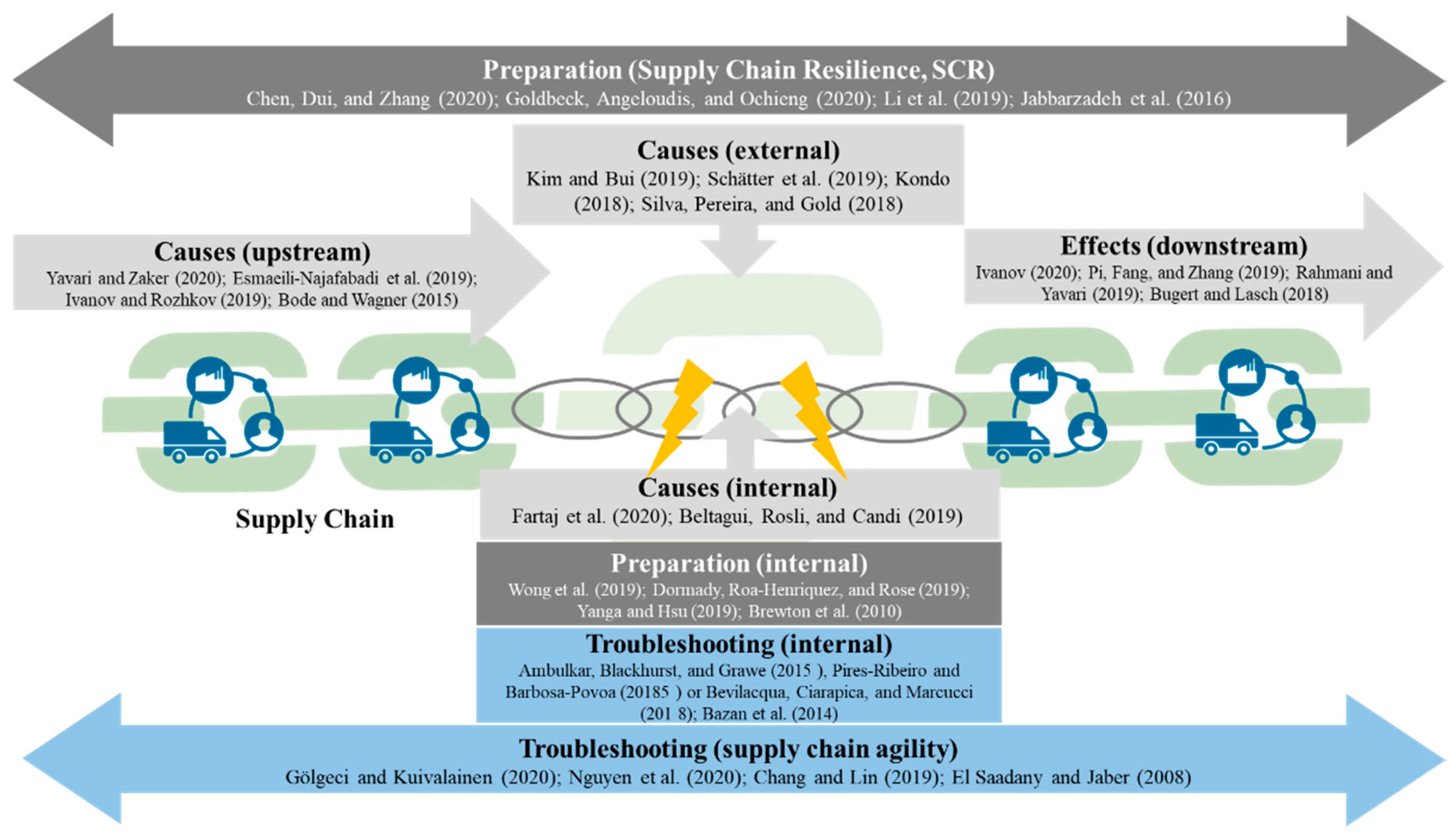
The theoretical framework regarding interruptions to supply chain and transportation processes can be structured according to Figure 1: Eight areas of management science research can be identified regarding supply chain interruptions, making up most of the research and practically relevant questions in relation to this subfield of supply chain management. As the eight relevant areas found from a literature analysis as described below, it can be recognized that the area of internal causes is under-represented and therefore under-researched. Our research is positioned exactly within this field and research gap and has the objective to further increase the knowledge about internal causes for supply chain disruptions and their effects. In order to achieve this, we analyze the specific internal case of computer system failures and the impacts on downstream supply chain processes. Additionally, the examined disruptions with internal causes take an explorative research perspective and do not focus on the impact of IT disruptions. Hence, we aspire to contribute to this research stream through our quantitative explanative research design.
From the above figure, we outline the described elements and levels in detail, as follows.
Preparation (Supply Chain Resilience, SCR): Resilience refers to the ability of supply chains to withstand disruptions and unexpected events, such as supply chain interruptions. This is exemplified, for example, by Chen, Dui and Zhang [5], suggesting a quantitative cost-based measure for overall supply chain resilience. This team of authors also discussed this aspect from different customer perspectives. Specific measures, e.g., repair capacities to increase resilience, are analyzed by Goldbeck, Angeloudis and Ochieng [19]. A dedicated network approach is presented by Li, Zobel, Seref and Chatfield [20] regarding a holistic supply chain resilience approach. This holistic supply chain resilience perspective is also addressed, for example, by Jabbarzadeh, Fahimnia, Sheu and Moghadam [3].
Preparation (internal): Wong, Lirn, Yang and Shang [4], for example, provide a vivid example of the questions related to firm-level preparation analysis and management approaches. They propose the application of organizational information process theory for preparing individual firms for supply chain disruptions. Furthermore, this research shows under which circumstances firm-level preparation and resilience pay off regarding specific performance measures. This is also connected to the production theory of individual forms, for example, in the work of Dormady, Roa-Henriquez and Rose [21]. Research outputs also address specific industries and sectors, for example, the maritime business sector [22]. A specific application of this form perspective to family-owned forms is presented by Brewton, Danes, Stafford and Haynes [23].
Causes (upstream) The upstream structure of supply chains can be the source of many disruption potentials in global value chains, as outlined, for example, by Bode and Wagner [24]. This is especially true for a supply chain with increased complexity, as shown in this research based on prediction models. Many publications shed light on the reasons for ripple effects and disruptions along the value chain, e.g., Esmaeili-Najafabadi, Fallah Nezhad, Pourmohammadi, Honarvar and Vahdatzad [25]; Ivanov and Rozhkov [26]; and Yavari and Zaker [27].
Causes (external): Discussions of external causes of supply chain disruptions mainly concentrate on grave events such as natural disasters and other “force majeure” events regarding supply chain management. This is shown, for example, by Kondo [28] for a powerful earthquake in Japan. Similar approaches are presented, e.g., by Silva, Pereira and Gold [29] for Brazil; Kim and Bui [30] for Puerto Rico; and Schätter, Hansen, Wiens and Schultmann [31] with regard to a general decision management approach to unexpected external events.
Causes (internal): Fartaj, Kabir, Eghujovbo, Ali and Paul [32] show for the automotive industry, transportation processes and also production logistics that internal causes can be a major source of process and supply chain disruptions. Nevertheless, disruptions not only stem from negative process deviations, but might also be caused by positive innovation changes, as Beltagui, Rosli and Candi [33] show for the introduction of 3D printing processes in firms.
Effects (downstream): A multitude of research works address the effects of interruptions and outages on supply chain management from a downstream perspective. For the 2020 COVID-19 crisis, this is exemplified by Ivanov [12] from a global perspective. Further research outputs highlight the role of demand disruptions in the context of supply chain resilience, e.g., Pi, Fang and Zhang [34]; Rahmani and Yavari [35]; and Bugert and Lasch [36].
Troubleshooting (internal): Some research contributions explore and show the benefits of firm-level mitigation measures for process and supply chain interruptions. A typical example is Bazan et al. (2014), who analyze the positive effects of production restoration operations under such critical conditions. This is further detailed by other publications such as Ambulkar, Blackhurst and Grawe [37]; Pires Ribeiro and Barbosa-Povoa [38]; and Bevilacqua, Ciarapica and Marcucci [39].
Troubleshooting (Supply Chain Agility): Regarding mitigation efforts after supply chain disruptions, El Saadany and Jaber [1], for example, describe how production interruptions can be managed in a two-tier setting. This aims to increase supply chain agility for disruption cases. Similar approaches are presented by Gölgeci and Kuivalainen [40] in the marketing domain; Nguyen, Sharkey, Wheeler, Mitchell and Wallace [41], proposing quantitative indicators; and Chang and Lin [42], regarding lead-time.
3. Data and Sample
To investigate the impact of information technology disruptions in retail logistics, we chose an empirical single-case study research design as one part of our field-based research. Additionally, we wished to delimit our approach from experimental investigations, as we did not influence variables, but rather observed their development within a real-world setting. Herein, we examine five warehouses belonging to a large German brick-and-mortar grocery retailer. While the retailer is operating 18 of these distribution centers, each of the observed warehouses is responsible for supplying between 341 and 522 grocery stores per day.
Wollenburg et al. (2018) elaborate several typologies for retailers operating within offline and online retailing channels [43]. According to their framework, we assigned the observed retail company to the type where offline and online operations are separated on the operational level and distribution centers solely pick and deliver orders for grocery stores. This is also commonly referred to as traditional brick-and-mortar grocery logistics. Therefore, we focus on the impact of information technology disruptions during the order fulfillment of offline demand and within the context of stationary grocery retailing.
In our case study, every distribution center receives goods from suppliers, stores them within the warehouse, picks orders that are sent to the supermarket stores and delivers picked stock keeping units (SKU) to the assigned grocery shops using transportation aids. Parallel to this material flow, the information flow is ensured through a warehouse management system and a route-planning system, as well as a track-and-trace system.
Taking the perspective of Porter’s value chain, we analyze the impact of information technology disruptions on the activity level of outbound logistics. Each of the examined warehouses has two major steps for order fulfillment: (1) order picking and (2) transport logistics. Although there are sub-units for each of these process steps, we choose the aggregation level of these two inter-organizational units, referred to as (1) the order-picking sector and (2) the transport sector, with the key processes being (1) warehouse logistical process and (2) truck loading, respectively.
The order-picking sector is responsible for complete, on-time order compiling based on the orders of the shops and uses a pick-by-voice technology where all order pickers wear a headset connected to a small wearable computer. The picking system names the storage location and the number of SKUs to pick. Successful picking operations are confirmed when pre-defined confirmation codes on the storage locations are correctly given back to the picking system, e.g., through linguistic input that can be identified by a speech recognition software running on the wearable computer, or by scanning barcode labels at the storage locations. Rolling cages and pallets are utilized as transportation aids. All data assigned to this process can be obtained through the company’s warehouse management system.
After the order-picking process, the rolling cages with SKUs are buffered at a shipping area and ready for distribution to the grocery stores. The transport sector is responsible for delivering the full amount of transport units within a given time window. All truck drivers use a mobile device to receive their work tasks, e.g., to load a certain number of containers for a grocery store and deliver them within a predefined time window. In order to fulfill the task, truck drivers have to scan all relevant 1D barcodes, which are attached to the containers, load them into the trucks, and record differences between the data provided by the mobile device and the condition of transported goods. All data assigned to this process can be obtained through the company’s track-and-trace system.
Due to the high level of digitalization and automation, the IT department is permanently measuring the functionality of the logistics systems. Errors that affect the operational logistics processes are reported by users or IT specialists through a management information system, which documents the strength of the computer system disruption, the number of affected employees and the duration of the disruption. Thus, computer system disruptions can be matched with the efficient progression of the warehouse processes during these outages.
In this paper, we investigate computer system disruptions related to the order picking sector, as well as disruptions related to the transport sector. The order picking sector is referred to as the warehouse logistics process and is understood as the first node in the network of relevant retail logistics operations. After this step, the transport logistics processes of truck loading represent the second node as an equivalent process step.
Our observations include the evaluation of efficiency for computer system disruptions regarding (1) the network as a whole and (2) the two nodes as isolated processes. The object of investigation is a computer system disruption within node 1 in the context of case 1 (C1) and a computer system disruption within node 2 in the context of C2. In each case, the computer system disruptions affect the core information system of the main process for one hour.
In C1, the picking system broke down for one hour, while, in C2, the track-and-trace system broke down for the same duration. During the breakdown, the employees tried to fulfill their work tasks without digital work equipment and fell back on paper-based picking and truck loading. The following chapter introduces and justifies the application of DEA as a key research method for measuring the efficiency impact of computer system disruptions in retail logistics.
4. Methodology
4.1. Method Selection
In general, DEA is a non-parametric optimization method of mathematical programming for measuring the relative efficiency of decision-making units (DMUs) that have multiple inputs and outputs. A basic model was introduced by Charnes, Cooper and Rhodes (1978) and is based on Pareto’s definition of economic efficiency [44] and Koopmans’ activity analysis concept [45], together with the publications of Debreu and Farrell, which deal with radial efficiency measurement [46,47].
Four characteristics of computer system disruptions justify the application of DEA as a key research method: (1) The impact is not predictable and is not yet examined from an efficiency-based point of view. As a result, there is no a priori knowledge about the functional relationships of new technologies towards humans. (2) Because computer system disruptions influence the human workforce, the theory of work systems is applied as a theoretical framework within the case analyses. As the achievement of work objectives requires inputs and produces outputs, a method that enables the integration of several in- and output factors along with the possibility of factor enhancement is needed. (3) Without the existence of a benchmark value for the level of efficiency in computer system disruption scenarios, the analysis has to compare the performance of the different empirical observations. (4) As it is unclear whether computer system disruptions spawn an immediate or gradual development of efficiency, the progress of efficiency in retail logistics is illustrated with an empirical curve progression.
Therefore, the results of the analysis have to be comparable between several periods. As DEA does not require a priori information (requirement 1), considers multiple measures (requirement 2) [48,49], compares only the different empirical observations (requirement 3) [50] and has comparable results when factors are constant (requirement 4) [48,49], it is the method of choice.
4.2. CCR and BCC Model
The optimization method can be based on constant returns to scale (CRS) in the CCR model named by its authors Charnes, Cooper and Rhodes [50] or variable returns to scale (VRS) in the BCC model named by its authors Banker, Charnes and Cooper [51], as well as each case with an input or output orientation. The mathematical formulation of the CCR model is [50]:
where:
= the weight given to the output r;
= amount of output r produced by DMU j;
= the weight given to input i;
= amount of input i used by DMU j;
n = the number of DMUs;
t = the number of outputs; m = the number of inputs;
ε = a small positive number.
The basic idea is to calculate an efficiency frontier that is used as a best practice input–output combination for the underlying production scenario. A score of 1.0 indicates that a DMU is efficient and positioned on the efficiency frontier, whereas the relative inefficiency of other DMUs can be determined by measuring the distance between individual DMU performance and the efficiency frontier. Measuring efficiency under the assumption of CRS is known as overall technical efficiency (OTE). This includes the determination of (in)efficiency based on (1) the input/output transformation, meaning pure technical efficiency (PTE), as well as (2) the size of operations, meaning scale efficiency (SE). This decomposition is possible under VRS [51,52,53].
As SE is a number without a unit between 0 and 1, an SE value of 1 means that the DMU is operating with the optimal operation size, and a difference of 1-SE determines the extent of the inefficiency arising from the non-optimal size of operations for a single DMU. A DMU that is efficient under CRS and VRS operates under the most productive scale size (MPSS), which is also used as a measure for the optimal size of the operation for all other DMUs. The BCC model can be mathematically expressed as:
ω = free (unconstrained in sign)
4.3. NDEA and Multi-Stage NDEA
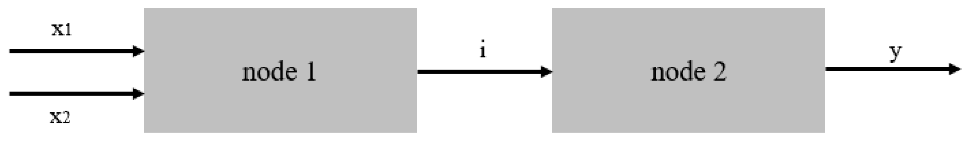
Conventional DEA models like those explained in the previous section, as well as methodological advancements, e.g., super efficiency to rank DMUs in DEA [54], DEA window analysis [55,56,57] and the DEA Malmquist index [58] for time series analysis, and fuzzy DEA for imprecise or vague input and output measures [59,60,61], use the black box assumption for describing DMUs. Therein, the internal structure of DMUs is ignored, and their performance is explained as a function resulting from the transformation of its input and output measures. This paradigm was dissolved by Färe and Primont [62], who presented a DEA model for multi-plant firms and applied it to a dataset of nineteen production plants from four firms operating coal-fired steam electric generating plants. For the first time, the internal structure of the company was not ignored, but was deconstructed into several plants. Over the years, Färe worked on several extensions for DEA models, evaluating the efficiency of DMUs with their known internal structure [63,64,65,66,67]. Thereby, Färe [64] was the first approach to deal with intermediate input variables that are used in several nodes of a network. Based on these approaches, NDEA was applied to measure the efficiency of banks, as a frequently used object of research in the DEA literature, by separating services and sales as two components of a banking system [68]. As the above-presented introduction of intermediate variables to the DEA methodology cannot be equated with establishing the logic of sequential nodes within one network, the development of two-stage DEA models is understood as a parallel stream of research and is of central interest in the course of this paper. Wang, Gopal and Zionts [69] developed a DEA model to assess the impact of IT on firm performance using two inputs, x1 and x2, for node 1. Connected with intermediate variable I, which acts as an output for node 1 and an input for node 2, the second stage has one output measure, y. Figure 2 illustrates the structure of the two-stage network DEA model applied in this paper.
A similar approach was presented by Seiford and Zhu [70], examining the performance of the top 55 U.S. commercial banks via a two-stage production process that separates profitability and marketability. NDEA and multi-stage NDEA is often applied in current research approaches for performance evaluation in supply chain management and logistics [71,72,73,74,75,76].
5. Formulation of a Multi-Stage NDEA Model
5.1. Specifications of Input-Output Measures
The specification of the DEA model begins with the selection of appropriate input and output measures that are used to calculate aggregated efficiency values per DMU and period, as well as per node in the network and for the network as a whole. Within the efficiency analysis, we evaluated the performance of five distribution centers that are used as DMUs. Since the efficiency analysis aspires to measure the impact of computer system disruptions on the operational processes in warehouse logistics, we treated the two key processes—order picking and transportation—as two separate nodes. As a first step, we define the input and output values for the order-picking process. The following input measures are applied to the order-picking efficiency model:
- Total picking time, I1: As order picking is a laborious and time-intensive warehouse process, the sum of total picking hours represents the human resources invested in the picking process. Focusing exclusively on the core process picking, this measurand indicates how well human resources utilize their work equipment. For the DEA model, the period of time between (a) receiving general order data from a picking system and (b) finishing a batch through transfer to the next workstation is considered. The data were extracted from the warehouse management system. Process delays through computer system disruptions could possibly occur and result in an extension of the total picking time and, as a consequence, be quantified by this input factor.
- Total number of batches, I2: Orders from the grocery stores are aggregated into batches through the warehouse management system, which is primarily premised on product groups and the assigned transportation aid. Hence, the total number of batches is an input factor that expresses the work amount for the picking department. On the other hand, computer system disruptions can lead to problems in replenishing storage locations through forklifts. This, in turn, generates a high number of additional batches that will significantly lower the key SKU figure per batch. Problems that may occur in relation to storage replenishment can therefore be quantified with this input measure.
- Total number of incoming pallets, I3: Supplies to the warehouse are measured as incoming pallets and can be understood as the primary resource for order picking. The total number of pallets is an input factor that expresses the workload for a warehouse and is independent of computer system disruptions. It is used as a control variable to ensure that the volatile demands of grocery stores can be considered when measuring the efficiency of a warehouse in retail logistics.
On the output side, the individual performance of order pickers can be measured by one indicator.
- Total SKUs picked, O1: Because the most important output of the order-picking process is the physically compiled orders, the units picked by the individual order picker are used as an output. However, as the total amount of picked units correlates with the first input (total picking time of order picker), which is inadmissible when applying DEA, the number of targeted storage locations is used.
Within the NDEA model, the intralogistics processes of order picking and truck loading are divided into two parts: the first with the objective of transforming picking time, batches, as well as incoming pallets into picked SKUs as an intermediate variable, and the second with the objective of transforming these intermediate variables into outputs of the truck loading process. Thus, the intermediate total SKUs picked connect the order picking and the truck loading process by process by acting as O1 in the upstream and as I1 in the downstream process. Furthermore, the following input and output measures are applied to the loading process efficiency model:
- Total loading time, I2: After registering at the responsible dispatcher in the logistics center, the professional truck drivers receive their route with the grocery stores to deliver to, as well as the loading gate, loading lane, time window, and the number of transportation aids on a mobile device. A handheld scanner is directly connected to the retailer’s track-and-trace system and is mainly used to digitally document the loading process by scanning all 1D barcodes on the assigned load carriers. The total loading time includes the period of time between scanning the first (t0) and the last (t1) load carrier.
- Total on-time deliveries to stores, O1: As one main goal of the transport unit is the on-time delivery to all customers, the total amount of stores that receive their goods punctually is a vital variable to monitor the success of the process. Furthermore, obstructions through computer system disruptions can extend process times in warehouse logistics, which can result in delayed deliveries. This makes O1 an important measurand for the network itself, as well as for the impacts of any computer system disruptions that may occur.
- Lost transport units, O2: The second goal of the transport unit is the complete delivery of all assigned transport units for the defined order date. As transportation aids are labeled with a 1D barcode and scanned at every relevant node of the warehouse material flow, lost transport units are rare in ordinary business. However, several kinds of operational distortions can interrupt the information flow of the warehouse. This leads, e.g., to transport units without information about the gate and lane at the end of the order-picking process, transport units sent to the wrong gates, or transport units that cannot be scanned during the loading process. The results of these exceptional cases are that the units cannot be found, are recorded as lost transportation units, and are delivered on the next delivery date. As DEA would consider a large number of lost transport units as a large output and, therefore, as highly efficient, O2 is integrated as an undesirable output.
The statistically equal distribution of these data attributes is essential, as significant inequalities could affect the quantitative analysis. Furthermore, the size of the warehouses, expressed through the number of batches, the number of picking hours, the total number of SKUs picked and loaded, and the total number of delivered customers, is of central importance. Table 1 summarizes the key attributes of the dataset by applying descriptive statistics. Furthermore, as the measures can only be applied if they are not highly correlated, a correlation matrix was calculated. The results indicate that there is no linear statistical relationship between the applied input and output measures.
5.2. Model Orientation, Type of Intermediate Variable, and Window Width
For an efficiency-oriented analysis of supply chain disruptions, we use the previously elaborated factors, whereby the DEA model aspires to (1) maximize desirable outputs, (2) minimize undesirable outputs, (3) maximize desirable inputs, or (4) minimize normal inputs [77]. In the course of this paper, reducing inputs is suitable for I1 and I2 in node 1, but not for I3. As we use the retailer’s warehouses as DMUs, it is doubtful that the warehouses can reduce the number of incoming pallets (I3) through warehouse optimization. Incoming goods result from the retailer’s orders to suppliers and, hence, are not reducible through operational warehouse processes. Maximizing the outputs, on the other hand, is suitable for node 1, as well as for node 2. Figure 3 illustrates the formulated NDEA model.
Regarding the warehouse processes in node 1, it is important to mention that the warehouse can operate on day n with batches assigned to day n and day n + 1. As a result, the total number of SKUs to pick is controllable and can be influenced by operational logistical processes. For node 2, the number of stores delivered to on time, O1, as well as the lost transport units, O2 (treated as an undesirable output), can be maximized by internal optimizations of the operational transport logistics processes. We chose an output-oriented DEA model. A third possibility would be a non-oriented model that allows input-increasing and output-decreasing options for a DMU to reach the constructed efficiency frontier. However, as we already excluded the input orientation, a non-oriented DEA is not applicable. Furthermore, an NDEA model can apply several assumptions regarding the orientation of the intermediate variable. It can operate as a free, fixed, non-increasing, non-decreasing, or item-specific variable. These settings can also be found in MaxDEA Pro. As the number of total SKUs picked changes during the transition from node 1 to node 2, we assume that the intermediate variable has a fixed orientation. Since we are aspiring to evaluate the impact of computer system disruptions based on panel data, we combined the formulated NDEA model with a DEA window analysis. Hence, the question of a suitable window width arises. As the analysis includes 17 days, which are treated as 17 periods within the panel dataset, whereby the computer system disruptions take place on day 5, we chose a window width of w = 4. The first window (W1–4) includes periods 1 to 4 and includes unobstructed operational processes, while the following periods are impacted by a computer system disruption.
To evaluate the impact of computer system disruptions on operational processes, we chose the investigation of panel data through a DEA window analysis. We included the day before the computer system disruption as t−n to compare the efficiency during the regular business to possible variations, the point in time of the computer system disruption as t0, and the consequential days as t+n to quantify the possible consequences for the operational efficiency.
6. Empirical Results and Analysis
6.1. C1: Computer System Disruptions in Order-Picking System Affecting Node 1
With the aim of quantifying the efficiency impact of computer system disruptions on operational processes in warehouse logistics, the first part of the analysis was carried out concerning the scale efficiency development of each DMU within the defined windows. To find out if CRS or VRS needed to be applied, CCR and BCC versions of the DEA model proposed earlier were calculated. The Table 2 summarizes the mean efficiency scores of the DEA model calculated with CRS and VRS, as well as the SE scores for the whole network and per DMU.
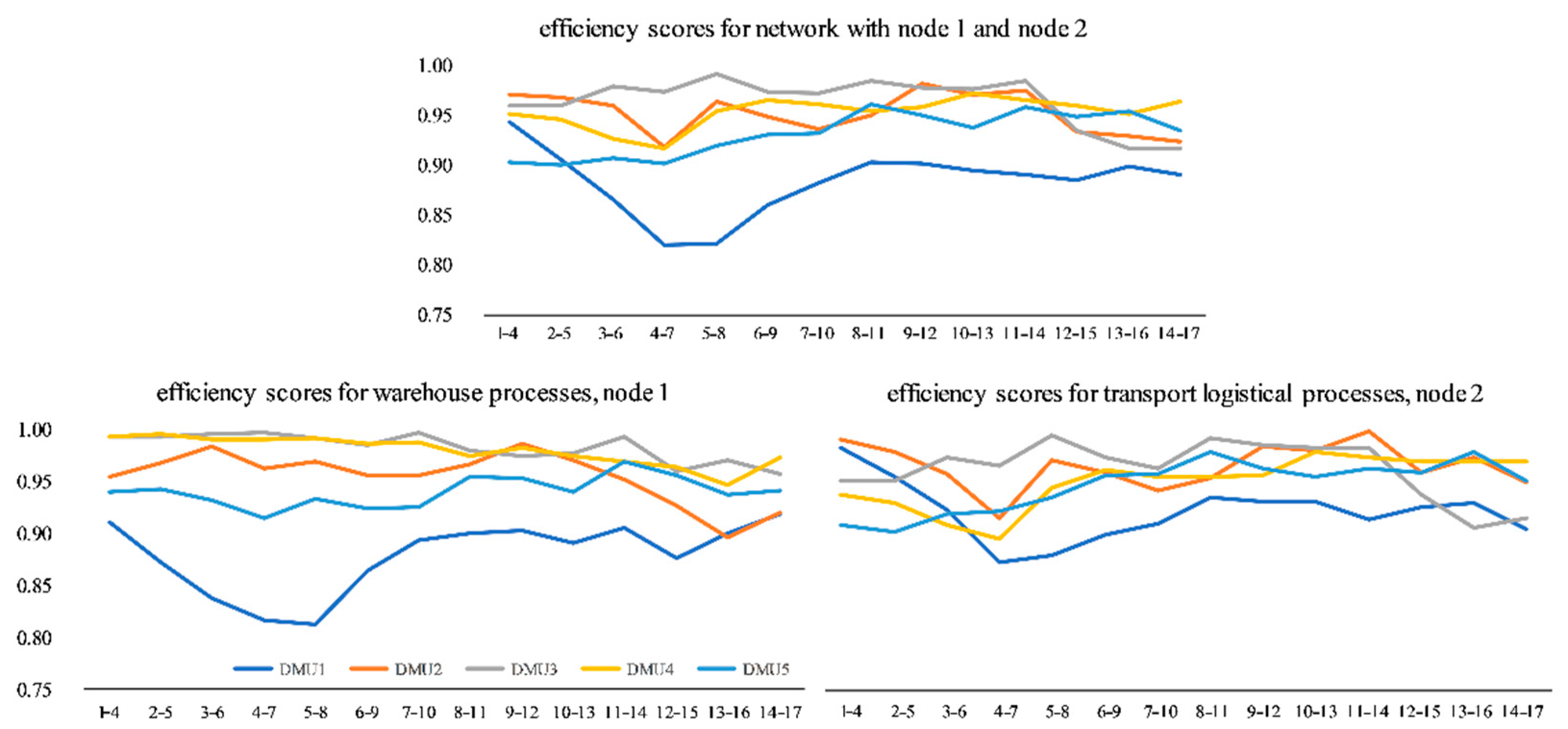
As the average SE score for all DMUs and in all windows is <1, the results indicate that the DMUs are not operating under MPSS. This becomes particularly clear when we consider that the individual warehouses can change their order picking and transport volume limits within a certain bound. As a result, a BCC model under the assumption of VRS must be applied within the methodological framework of a DEA window analysis. When considering the efficiency scores, the DMUs without computer system disruptions are constant, with a standard deviation of 0.02 (DMU2), 0.02 (DMU3), 0.01 (DMU4), and 0.02 (DMU5). DMU 1, on the other hand, has a standard deviation of 0.03 among all windows and 0.05 for W1–4 without a computer system disruption and W4–7 immediately after the computer system disruption. Besides the efficiency of the whole network, the developments of the single notes are of special interest when answering the research question. MaxDEA Pro enables the calculation of isolated efficiency values per DMU and node. The following figure visualizes, summarizes, and contrasts the efficiency scores per DMU and window for (1) the whole network, (2) the warehouse processes as node 1, and (3) the transport logistical processes as node 2.
The results illustrated in Figure 4 show that the computer system disruption in the warehouse logistics process takes place on day five and is therefore included in the efficiency score since W2–5 significantly reduces the efficiency of the whole network. The lowest efficiency level is reached in W4–7 and W5–8 immediately after the outage, so it is important to mention that the network efficiency of DMU 1 does not return to the original level before the disruption. Considering the single nodes, the warehouse logistics process is mainly influenced, which is not surprising in itself, as it was the epicenter of the computer system disruption. An interesting development can be found for the transport logistical process (node 2): (1) Although this subsequent process is not directly influenced by the disruption, the efficiency score drops at the same time as in the warehouse process; (2) the efficiency loss is not as grave as in node 1; and (3) node 2 recovers significantly faster to a higher and more stable efficiency level than node 1.
6.2. C2: Computer System Disruptions in Track-and-Trace Systems Affecting Node 2
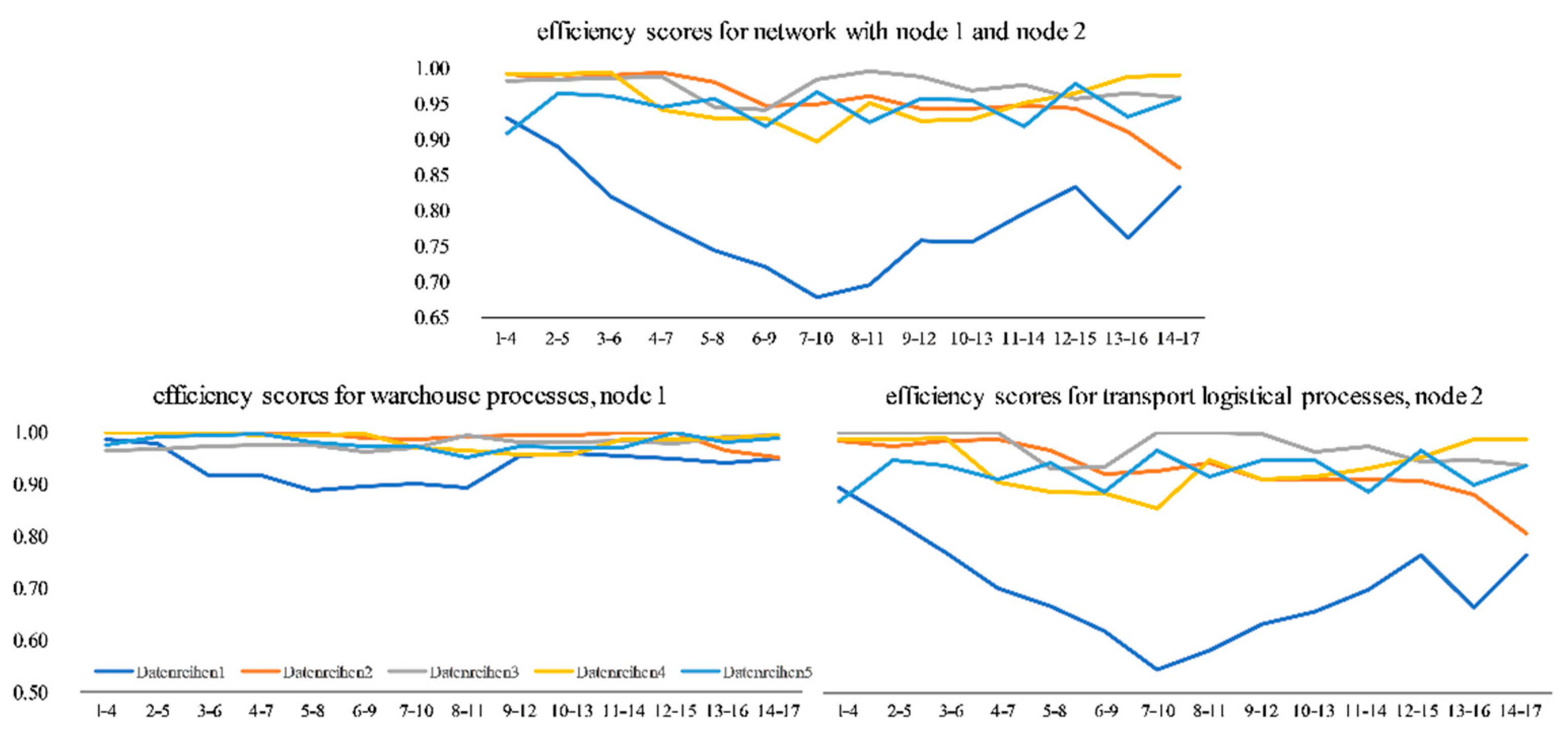
Considering that the decision to apply CRS or VRS was already discussed in the previous section, the investigation of a computer system disruption in the track-and-trace system affecting node 2 uses the same DEA model as C1. Figure 5 visualizes, summarizes, and contrasts the efficiency scores per DMU and window for (1) the whole network, (2) the warehouse processes as node 1, and (3) the transport logistical processes of node 2.
The curve progression of the total network evaluation in Figure 5 indicates a significantly decreasing efficiency level after the computer system disruption on day five over the course of the first week. The bottom is reached in W7–10 with an average efficiency score of 0.67 after starting at 0.93 in W1–4. A significant decrease is especially notable after the computer system disruption in W5–8, W6–9, and W7–10. By considering each node, it can be observed that the transport logistical process was mainly influenced, which is not surprising as it is the epicenter of the computer system disruption, with a drop from 0.87 in W2–5 to 0.46 in W7–10. Two circumstances deserve closer attention: (1) the length and duration of the curve drop are identical for the entire network and for node 1, and (2) a surprising finding can be stated when considering the efficiency progression of the warehouse processes. This upstream process is directly affected by the disruption of the track-and-trace system, although there is no material or information flow in the upstream direction. The efficiency drop is statistically not as severe as in the directly affected process, but is still noticeable, with a decline from 0.99 in W1–4 to 0.89 in W5–8.
7. Discussion
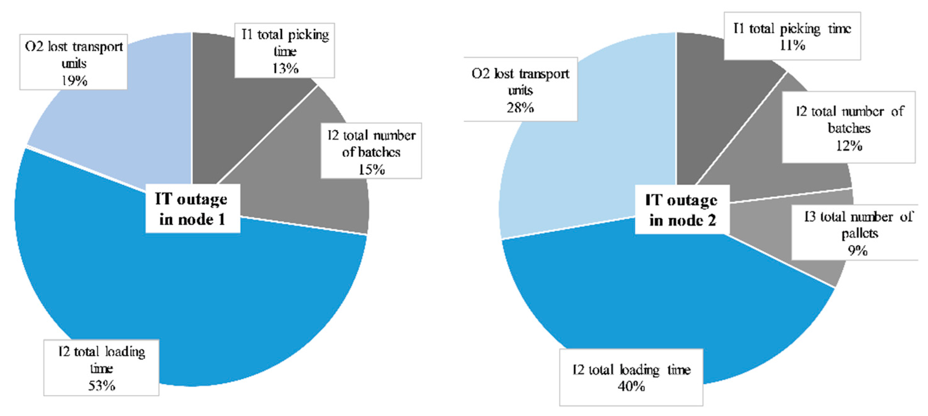
To provide a deeper understanding of the reasons for inefficiencies during computer system disruptions in retail logistics, we investigated the contribution of all input and output factors on the given efficiency scores. We thereby analyzed the number of non-zero input and output slacks, which is frequently applied in the context of DEA methodology after presenting a radial efficiency score improvement [78]. Depending on the orientation of the DEA model, slack-based measurements quantify the possibility of DMUs maximizing output values or minimizing input values that go beyond the radial projection of the envelopment model (CCR or BCC model). For the specific cases analyzed in C1 and C2, slack-based measurement can provide in-depth insights into which input or output factor is mainly responsible for inefficiencies. It is essential to mention that the slack-based measurement is calculated for the whole network of the NDEA model and not for single nodes. The following figure illustrates the results of the slack-based measurement for the computer system disruption in node 1 (C1, colored in grey) and in node 2 (C2, colored in blue).
The pie chart in Figure 6 on the left illustrates the proportion of possible optimizations per input and output factor for the case of a computer system disruption in the order-picking system (node 1). Therein, it is surprising that only 28% of the possible optimizations may come from the epicenter of the computer system disruption, namely the order-picking system (grey). Most of the inefficiencies result from the subsequent process, the transport logistical work system of truck loading. Increasingly high loading times and high numbers of lost transport units are, therefore, the main drivers of inefficiencies after a breakdown in the order-picking system. This deviation becomes clear when remembering the processes described in the data and sample section. An outage within the order-picking system may result in transportation aids with incomplete, wrong, or missing 1D barcodes. This leads to a media disruption of the digital workflow, consisting of scanning barcodes for the information flow. At this point, one finding deserves special attention: as the computer system disruption in node 1 leads to high inefficiencies regarding the I2 and O2 of node 2, the information workflow that is based on digital technology has a major impact on the efficiency of the retail operational processes in warehouse logistics. As seen in the right pie chart, the computer system disruption in node 2 leads to situations in which mainly I2 and O2 of node 2 could be minimized/maximized in order to reach the efficiency frontier. This also supports the efficiency progression in the previous chapter, which highlighted the low impact of the computer system disruption in node one on the previous order-picking process. However, it may be surprising that disruptions in the track-and-trace system lead to inefficiencies caused by the total picking time (I1, node 1). In operational logistics, a massively slowed loading process results in a significantly lower material flow of all goods leaving the warehouse. Consequently, the continuous working material flow of picked SKUs collides with the space that is still blocked in the outgoing goods department. This consequently slows down the order picker when moving at rack ends or changing aisles.
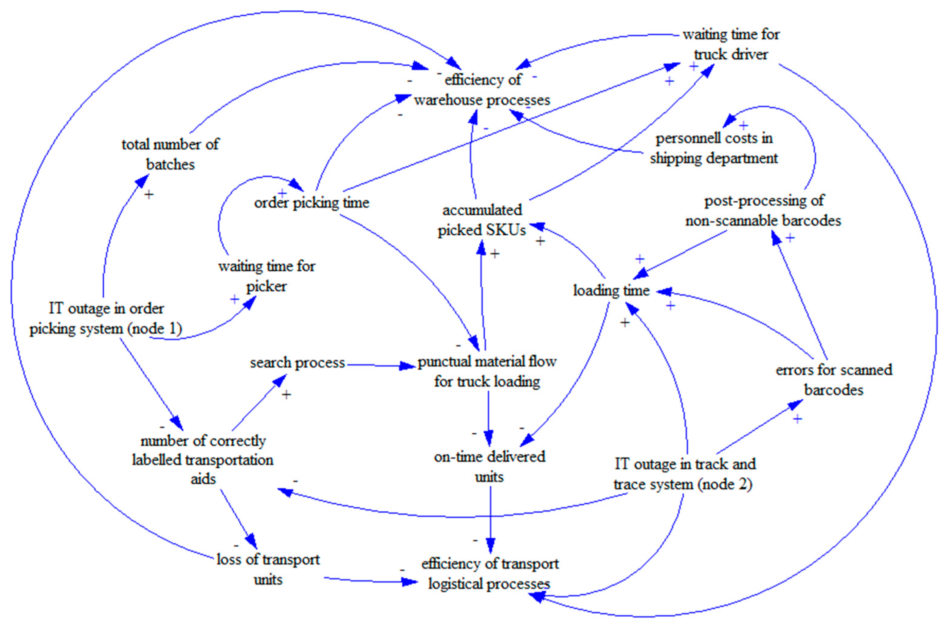
The complex and versatile interaction of warehouse and transport logistical processes during computer system disruptions is summarized in a system dynamics framework. The system dynamics methodology, developed by Jay W. Forrester in the 1950s as industrial dynamics, initially aimed to solve problems related to top management [79]. The methodology includes “[…] a perspective and set of conceptual tools that enable us to understand the structure and dynamics of complex systems” [80], p. VII. As management problems contain various elements in several systems and sub-systems interacting with one another, system dynamics abstracts these elements, takes an aggregated view, and captures the dynamic behavior of a system over time by mathematical modeling and visualization. Causal loop diagrams have been applied to shed light on the interplay and resulting mechanisms of various variables and levels in complex systems by visualizing a reference model [80]. The variables are connected to influence lines, forming causal chains and indicating whether the affected variable is influenced positively (+) or affected negatively (−). One example of a causal chain is as follows: A computer system disruption in the track-and-trace system leads to an increasing number of errors when scanning barcodes, which, as a consequence, requires a post-processing step for non-scannable barcodes. This additional process enlarges the loading time and decreases the number of units delivered on time. Finally, this has a negative impact on the efficiency of transport logistical processes.
We augment our quantitative and mostly static DEA methodology with the flexible system dynamics approach as an additional qualitative method to summarize the complex problem of computer system disruptions, consisting of various explanations on multiple levels. This allows us to integrate additional variables and factors that we were not able to include in our multivariate DEA approach, which may be due to data availability or restrictions of the applied methodology. Furthermore, the combination of these methodologies enables a further and deeper discussion of the problem structure and aims to provide new insights. As a basis for further deviations, we use the quantitative findings of our DEA model regarding the disruptions in different nodes of the logistics system. For further research, the system dynamics approach may again serve as a basis for an additional quantitative analysis of the examined system, as the relationships mapped in our framework can be transformed into mathematical equations.
These results link to existing research outputs and publications, for example, in the domain of resilience [81]. In particular, the link between sustainability and resilience is explored by these authors. Another example of where this paper connects to the existing literature is the interrelation between economic sustainability and resilience as the ability to withstand disruptions with adequate resources [82]. Furthermore, this links to resilience and even growth options in times of crisis due to critical infrastructure being a basic resource in relation to individual corporate capacities for change [83].
We can also connect the sustainability dimension of the resilience provided by corporate actors, vice versa, to their ability to establish long-term sustainability [84,85]. This, again, is connected to the public resource of resilience management, as outlined in [86].
Taking the results from the presented NDEA analysis as well as the systems dynamics model in Figure 7 towards a comparison with established resilience research, we arrive at the following observations:
First, ripple and subsequent effects of disruptions are a major field of analysis like for example described by Hosseini and Ivanov in 2020 [87]. In this paper, we report that in a quantitative (NDEA) and qualitative (system dynamics) was for such ripple or process effects. For example, in the above figure, we can recognize that disruptions in many cases lead to increased waiting times of workers (order pickers, truck drivers), increasing the operational and efficiency impact of disruptions originating, for example, from IT systems. This connects also to the observation by Gölgeci and Kuivalainen (2020) that social capital could be an important mediating and mitigating factor in resilience and disruption management [40].
Second, the “quantitative push” in resilience research is followed in our paper with the reference to the NDEA efficiency analysis to evaluate supply chain disruptions; this also represents the final factor in the qualitative system dynamics perspective (“efficiency of warehouse/transport processes”). Other research papers apply, for example, value-at-risk analytics like by Dixit et al. 2020 [88], financial impact measures like with Yu et al. in 2019 [89] or the general overview by Aldrighetti et al. in 2021 regarding costs of disruptions and low resilience levels in supply chains [90]. The most general and generic view on metrics for resilience analysis and management is provided by Behzadi et al. in 2020 [91].
Third, technology use is discussed as a driver as well as mitigation perspective for supply chain disruptions and resilience as was the original starting question for this paper: Gu et al. provide 2021 a similar approach [92], whereas Lohmer et al. in 2020 see, for example, blockchain technology as a possible moderator in supply chain disruptions and resilience [93]. Finally, Al-Talib et al. in 2020 describe how to apply digital IoT technologies to improve supply chain resilience [94].
In total, there is a considerate body of literature where the presented paper fits well into the main discussion streams with the presented messages and results. From a general perspective [95], focusing on specialized areas such as retail [96] up to the challenge of a generalized theory contribution in this field [4]—all aspects are addressed. This is the basis for further interactions and research addressing the challenges of supply chain resilience.
8. Conclusions
The quantitative results from this study showed specific but diverse efficiency impacts by technical computer system disruptions in the two stages of the operational retail logistics process. Considering performance measurement in supply chain management, Agrell and Hatami-Marbini [97] differentiate between (1) performance measurement that provides productivity estimations in the sense of prediction, e.g., yields, or demands, and (2) providing targets for improvement in the case of poor performance as a normative paradigm.
The findings of this paper can be assigned to a normative rather than a predictive paradigm, as they provide a deeper understanding of decreasing performance after computer system disruptions in operational retail logistics processes. For the research questions raised at the beginning, the findings show that supply chain disruptions are operationalizable on a micro-level and through a multi-variable approach. The quantitative DEA methodology applied in this paper takes an a posteriori evaluation perspective, which is a counterbalance to recent research in supply chain management focusing on the a priori simulations of disruption, e.g., related to COVID-19. Especially for logistics and supply chain managers, these evaluation approaches are valuable for scenarios, where disruptions may occur more than once. In most cases, technological disruptions are recurring. Therefore, our approach can be used to estimate costs and benefits for IT system reliability.
From a theoretical viewpoint, our results can be connected to the research results of Fartaj, Kabir, Eghujovbo, Ali and Paul [32] or Beltagui, Rosli and Candi [33] for internal causes of supply chain disruptions. In this sense, our research adds a further internal cause analysis regarding computer system breakdowns as internal disruptions of supply chain processes. Therefore, the existing theory and body of knowledge is expanded for this specific topical area.
The limitations of this study include its use of specific input and output types in one particular retail logistics setting. In addition, a specified setting in Germany is addressed; other countries’ cases and datasets could increase the geographical reach of such efficiency perspectives on supply chain disruptions. From a methodological point of view, we applied a traditional VRS-based DEA approach. As this requires the availability of exactly known values for the specified input and output measures, it is a deterministic method. Hatami-Marbini, Agrell, Fukuyama, Gholami and Khoshnevis [98] argue that this kind of model is susceptible to changes or errors in data values. As the data in real-world problems are sometimes imprecise or vague, they propose the application of fuzzy DEA as a more probabilistic model [61].
This study can be the basis for further research directed at showing similar effects for further processes in the supply chain and logistics management using the NDEA methodology. Additional analyses could also be directed at identifying new relevant explaining factors for the severity of efficiency losses and capacities for recovering (resilience). This could complement the predominantly qualitative research on supply chain resilience in the future.
From a practitioner’s point of view, this paper is dedicated to a non-parametric evaluation model to assess ex-post effects on the technical efficiency of operational processes in warehouse and transport logistics as a result of computer system disruptions. A potential ex ante approach could positively impact the decision-making process of logistic managers when it comes to the specification of the degree of availability [99], as well as the maximum degree of failure for computer system disruptions in logistics [100]. However, this is often a decision based on (rather short-term) cost considerations and seldom based on the overall long-term efficiency of operational production and logistics systems [101]. Therefore, further research is warranted in this interesting field, as highlighted by the disruptions to many supply chain processes caused by the COVID-19 pandemic.
Author Contributions
Conceptualization, M.K.; methodology, D.L.; software, D.L.; validation, M.K.; formal analysis, D.L.; investigation, D.L.; data curation, D.L.; writing—original draft preparation, D.L., M.K.; writing—review and editing, M.K.; visualization, D.L.; supervision, M.K. All authors have read and agreed to the published version of the manuscript.
Funding
This research received no external funding.
Institutional Review Board Statement
Ethical review and approval were waived for this study, due to the fact that we used anonymous data that was not retractable to individuals at any time.
Informed Consent Statement
Patient consent was waived due to the fact that we used anonymous data that was not retractable to individuals at any time.
Data Availability Statement
No data provided.
Conflicts of Interest
The authors declare no conflict of interest.
References
- El Saadany, A.M.; Jaber, M.Y. Coordinating a two-level supply chain with production interruptions to restore process quality. Comput. Ind. Eng. 2008, 54, 95–109. [Google Scholar] [CrossRef]
- Bazan, E.; Jaber, M.Y.; Zanoni, S.; Zavanella, L.E. Vendor Managed Inventory (VMI) with Consignment Stock (CS) agreement for a two-level supply chain with an imperfect production process with/without restoration interruptions. Int. J. Prod. Econ. 2014, 157, 289–301. [Google Scholar] [CrossRef]
- Jabbarzadeh, A.; Fahimnia, B.; Sheu, J.B.; Moghadam, H.S. Designing a supply chain resilient to major disruptions and supply/demand interruptions. Transp. Res. Part B Methodol. 2016, 94, 121–149. [Google Scholar] [CrossRef]
- Wong, C.W.; Lirn, T.C.; Yang, C.C.; Shang, K.C. Supply chain and external conditions under which supply chain resilience pays: An organizational information processing theorization. Int. J. Prod. Econ. 2020, 226, 107610. [Google Scholar] [CrossRef]
- Chen, L.; Dui, H.; Zhang, C. A resilience measure for supply chain systems considering the interruption with the cyber-physical systems. Reliab. Eng. Syst. Saf. 2020, 199, 106869. [Google Scholar] [CrossRef]
- Gaur, J.; Amini, M.; Rao, A.K. The impact of supply chain disruption on the closed-loop supply chain configuration profit: A study of sourcing policies. Int. J. Prod. Res. 2020, 58, 5380–5400. [Google Scholar] [CrossRef]
- Jahani, H.; Abbasi, B.; Hosseinifard, Z.; Fadaki, M.; Minas, J.P. Disruption risk management in service-level agreements. Int. J. Prod. Res. 2021, 59, 226–244. [Google Scholar] [CrossRef]
- Liu, M.; Liu, Z.; Chu, F.; Zheng, F.; Chu, C. A new robust dynamic Bayesian network approach for disruption risk assessment under the supply chain ripple effect. Int. J. Prod. Res. 2021, 59, 265–285. [Google Scholar] [CrossRef]
- Macdonald, J.R.; Zobel, C.W.; Melnyk, S.A.; Griffis, S.E. Supply chain risk and resilience: Theory building through structured experiments and simulation. Int. J. Prod. Res. 2018, 56, 4337–4355. [Google Scholar] [CrossRef]
- Han, J.; Shin, K. Evaluation mechanism for structural robustness of supply chain considering disruption propagation. Int. J. Prod. Res. 2016, 54, 135–151. [Google Scholar] [CrossRef]
- Dong, E.; Du, H.; Gardner, L. An interactive web-based dashboard to track COVID-19 in real time. Lancet Infect. Dis. 2020, 20, 533–534. [Google Scholar] [CrossRef]
- Ivanov, D. Predicting the impacts of epidemic outbreaks on global supply chains: A simulation-based analysis on the coronavirus outbreak (COVID-19/SARS-CoV-2) case. Transp. Res. Part E Logist. Transp. Rev. 2020, 136, 101922. [Google Scholar] [CrossRef] [PubMed]
- Kaplan, E.H. Containing 2019-nCoV (Wuhan) coronavirus. Health Care Manag. Sci. 2020, 23, 311–314. [Google Scholar] [CrossRef] [PubMed]
- Ivanov, D.; Dolgui, A. Low-Certainty-Need (LCN) supply chains: A new perspective in managing disruption risks and resilience. Int. J. Prod. Res. 2019, 57, 5119–5136. [Google Scholar] [CrossRef] [Green Version]
- Jabbarzadeh, A.; Fahimnia, B.; Sabouhi, F. Resilient and sustainable supply chain design: Sustainability analysis under disruption risks. Int. J. Prod. Res. 2018, 56, 5945–5968. [Google Scholar] [CrossRef]
- Ralston, P.; Blackhurst, J. Industr. 4.0 and resilience in the supply chain: A driver of capability enhancement or capability loss? Int. J. Prod. Res. 2020, 58, 5006–5019. [Google Scholar] [CrossRef]
- Zsidisin, G.A.; Petkova, B.N.; Dam, L. Examining the influence of supply chain glitches on shareholder wealth: Does the reason matter? Int. J. Prod. Res. 2016, 54, 69–82. [Google Scholar] [CrossRef]
- Pires, M.; Camanho, A.; Amorim, P. Solving the grocery backroom sizing problem. Int. J. Prod. Res. 2020, 58, 5707–5720. [Google Scholar] [CrossRef]
- Goldbeck, N.; Angeloudis, P.; Ochieng, W. Optimal supply chain resilience with consideration of failure propagation and repair logistics. Transp. Res. Part E: Logist. Transp. Rev. 2020, 133, 101830. [Google Scholar] [CrossRef]
- Li, Y.; Zobel, C.W.; Seref, O.; Chatfield, D. Network characteristics and supply chain resilience under conditions of risk propagation. Int. J. Prod. Econ. 2020, 223, 107529. [Google Scholar] [CrossRef]
- Dormady, N.; Roa-Henriquez, A.; Rose, A. Economic resilience of the firm: A production theory approach. Int. J. Prod. Econ. 2019, 208, 446–460. [Google Scholar] [CrossRef]
- Yang, C.-C.; Hsu, W.-L. Evaluating the impact of security management practices on resilience capability in maritime firms—A relational perspective. Transp. Res. Part A Policy Pract. 2019, 110, 220–233. [Google Scholar] [CrossRef]
- Brewton, K.E.; Danes, S.M.; Stafford, K.; Haynes, G.W. Determinants of rural and urban family firm resilience. J. Fam. Bus. Strategy 2010, 1, 155–166. [Google Scholar] [CrossRef]
- Bode, C.; Wagner, S.M. Structural drivers of upstream supply chain complexity and the frequency of supply chain disruptions. J. Oper. Manag. 2015, 36, 215–228. [Google Scholar] [CrossRef]
- Esmaeili-Najafabadi, E.; Nezhad, M.S.F.; Pourmohammadi, H.; Honarvar, M.; Vahdatzad, M.A. A joint supplier selection and order allocation model with disruption risks in centralized supply chain. Comput. Ind. Eng. 2019, 127, 734–748. [Google Scholar] [CrossRef]
- Ivanov, D.; Rozhkov, M. Disruption tails and post-disruption instability mitigation in the supply chain. IFAC-PapersOnLine 2019, 52, 343–348. [Google Scholar] [CrossRef]
- Yavari, M.; Zaker, H. Designing a resilient-green closed loop supply chain network for perishable products by considering disruption in both supply chain and power networks. Comput. Chem. Eng. 2020, 134, 106680. [Google Scholar] [CrossRef]
- Kondo, A. The effects of supply chain disruptions caused by the Great East Japan Earthquake on workers. Jpn. World Econ. 2018, 47, 40–50. [Google Scholar] [CrossRef] [Green Version]
- Silva, M.E.; Pereira, S.C.; Gold, S. The response of the Brazilian cashew nut supply chain to natural disasters: A practice-based view. J. Clean. Prod. 2018, 204, 660–671. [Google Scholar] [CrossRef]
- Kim, K.; Bui, L. Learning from Hurricane Maria: Island ports and supply chain resilience. Int. J. Disaster Risk Reduct. 2019, 39, 101244. [Google Scholar] [CrossRef]
- Schätter, F.; Hansen, O.; Wiens, M.; Schultmann, F. A decision support methodology for a disaster-caused business continuity management. Decis. Support Syst. 2019, 118, 10–20. [Google Scholar] [CrossRef]
- Fartaj, S.R.; Kabir, G.; Eghujovbo, V.; Ali, S.M.; Paul, S.K. Modeling transportation disruptions in the supply chain of automotive parts manufacturing company. Int. J. Prod. Econ. 2020, 222, 107511. [Google Scholar] [CrossRef]
- Beltagui, A.; Rosli, A.; Candi, M. Exaptation in a digital innovation ecosystem: The disruptive impacts of 3D printing. Res. Policy 2019, 49, 103833. [Google Scholar] [CrossRef]
- Pi, Z.; Fang, W.; Zhang, B. Service and pricing strategies with competition and cooperation in a dual-channel supply chain with demand disruption. Comput. Ind. Eng. 2019, 138, 106130. [Google Scholar] [CrossRef]
- Rahmani, K.; Yavari, M. Pricing policies for a dual-channel green supply chain under demand disruptions. Comput. Ind. Eng. 2019, 127, 493–510. [Google Scholar] [CrossRef]
- Bugert, N.; Lasch, R. Effectiveness of responsive pricing in the face of supply chain disruptions. Comput. Ind. Eng. 2018, 124, 304–315. [Google Scholar] [CrossRef]
- Ambulkar, S.; Blackhurst, J.; Grawe, S. Firm’s resilience to supply chain disruptions: Scale development and empirical examination. J. Oper. Manag. 2015, 33–34, 111–122. [Google Scholar] [CrossRef]
- Pires Ribeiro, J.; Barbosa-Povoa, A. Supply Chain Resilience: Definitions and quantitative modelling approaches—A literature review. Comput. Ind. Eng. 2018, 115, 109–122. [Google Scholar] [CrossRef]
- Bevilacqua, M.; Ciarapica, F.E.; Marcucci, G. A modular analysis for the Supply Chain Resilience Triangle. IFAC-PapersOnLine 2018, 51, 1528–1535. [Google Scholar] [CrossRef]
- Gölgeci, I.; Kuivalainen, O. Does social capital matter for supply chain resilience? The role of absorptive capacity and marketing-supply chain management alignment. Ind. Mark. Manag. 2020, 84, 63–74. [Google Scholar] [CrossRef]
- Nguyen, H.; Sharkey, T.C.; Wheeler, S.; Mitchell, J.E.; Wallace, W.A. Towards the development of quantitative resilience indices for Multi-Echelon Assembly Supply Chains. Omega 2021, 99, 102199. [Google Scholar] [CrossRef]
- Chang, W.-S.; Lin, Y.-T. The effect of lead-time on supply chain resilience performance. Asia Pac. Manag. Rev. 2019, 24, 298–309. [Google Scholar] [CrossRef]
- Wollenburg, J.; Hübner, A.; Kuhn, H.; Trautrims, A. From bricks-and-mortar to bricks-and-clicks: Logistics networks in omni-channel grocery retailing. Int. J. Phys. Distrib. Logist. Manag. 2018, 48, 415–438. [Google Scholar] [CrossRef]
- Pareto, V. Cours d’économie Politique; Librairie Droz: Paris, France, 1897. [Google Scholar]
- Koopmans, T.C. An analysis of production as an efficient combination of activities. In Activity Analysis of Production and Allocation; Koopmans, T.C., Ed.; Wiley: London, UK, 1951; pp. 33–97. [Google Scholar]
- Farrell, M.J. The measurement of productive efficiency. J. R. Stat. Soc. 1957, 120, 253–290. [Google Scholar] [CrossRef]
- Debreu, G. The coefficient of resource utilization. Econometrica 1951, 19, 273–292. [Google Scholar] [CrossRef]
- Cooper, W.W.; Seiford, L.M.; Tone, K. Data Envelopment Analysis: A Comprehensive Text with Models, Applications, References and DEA-Solver Software; Springer: Boston, MA, USA, 2007. [Google Scholar]
- Cooper, W.W.; Seiford, L.M.; Zhu, J. Data Envelopment Analysis: History, Models, and Interpretations. In Handbook on Data Envelopment Analysis; Cooper, W.W., Seiford, L.M., Zhu, J., Eds.; Springer: Boston, MA, USA, 2011; pp. 1–39. [Google Scholar]
- Charnes, A.; Cooper, W.W.; Rhodes, E. Measuring the efficiency of decision making units. Eur. J. Oper. Res. 1978, 2, 429–444. [Google Scholar] [CrossRef]
- Banker, R.D.; Charnes, A.; Cooper, W.W. Some models for estimating technical and scale inefficiencies in Data Envelopment Analysis. Manag. Sci. 1984, 30, 1078–1092. [Google Scholar] [CrossRef] [Green Version]
- Banker, R.D. Estimating most productive scale size using data envelopment analysis. Eur. J. Oper. Res. 1984, 17, 35–44. [Google Scholar] [CrossRef]
- Banker, R.D.; Cooper, W.W.; Seiford, L.M.; Zhu, J. Returns to scale in DEA. In Handbook on Data Envelopment Analysis; Cooper, W.W., Seiford, L.M., Zhu, J., Eds.; Springer: Boston, MA, USA, 2011; pp. 41–70. [Google Scholar]
- Andersen, P.; Petersen, N.C. A Procedure for Ranking Efficient Units in Data Envelopment Analysis. Manag. Sci. 1993, 39, 1261–1264. [Google Scholar] [CrossRef]
- Charnes, A.; Clark, C.T.; Cooper, W.W.; Golany, B. A developmental study of data envelopment analysis in measuring the efficiency of maintenance units in the U.S. air forces. Ann. Oper. Res. 1985, 2, 95–112. [Google Scholar] [CrossRef]
- Halkos, G.E.; Tzeremes, N.G. Exploring the existence of Kuznets curve in countries’ environmental efficiency using DEA window analysis. Ecol. Econ. 2009, 68, 2168–2176. [Google Scholar] [CrossRef]
- Jia, T.; Yuan, H. The application of DEA (Data Envelopment Analysis) window analysis in the assessment of influence on operational efficiencies after the establishment of branched hospitals. BMC Health Serv Res 2017, 17, 265. [Google Scholar] [CrossRef] [PubMed]
- Malmquist, S. Index numbers and indifference surfaces. Trab. De Estad. 1953, 4, 209–242. [Google Scholar] [CrossRef]
- Sengupta, J.K. A fuzzy systems approach in data envelopment analysis. Comput. Math. Appl. 1992, 24, 259–266. [Google Scholar] [CrossRef] [Green Version]
- Sengupta, J.K. Measuring efficiency by a fuzzy statistical approach. Fuzzy Sets Syst. 1992, 46, 73–80. [Google Scholar] [CrossRef]
- Hatami-Marbini, A.; Emrouznejad, A.; Tavana, M. A taxonomy and review of the fuzzy data envelopment analysis literature: Two decades in the making. Eur. J. Oper. Res. 2011, 214, 457–472. [Google Scholar] [CrossRef]
- Färe, R.; Primont, D. Efficiency measures for multiplant firms. Oper. Res. Lett. 1984, 3, 257–260. [Google Scholar] [CrossRef]
- Färe, R.; Grosskopf, S. Network DEA. Socio-Econ. Plan. Sci. 2000, 34, 35–49. [Google Scholar] [CrossRef]
- Färe, R. Measuring Farrell efficiency for a firm with intermediate inputs. Acad. Econ. Pap. 1991, 19, 329–340. [Google Scholar]
- Färe, R.; Whittaker, G. An Intermediate Input Model of Dairy Production Using Complex Survey Data. J. Agric. Econ. 1995, 46, 201–213. [Google Scholar] [CrossRef]
- Färe, R.; Grosskopf, S. Intertemporal Production Frontiers: With Dynamic DEA; Springer: Dordrecht, The Netherlands, 1996. [Google Scholar]
- Färe, R.; Grosskopf, S. Productivity and intermediate products: A frontier approach. Econ. Lett. 1996, 50, 65–70. [Google Scholar] [CrossRef]
- Cook, W.D. Multicomponent Efficiency Measurement and Shared Inputs in Data Envelopment Analysis: An Application to Sales and Service Performance in Bank Branches. J. Product. Anal. 2000, 14, 209–224. [Google Scholar] [CrossRef]
- Wang, C.H.; Gopal, R.D.; Zionts, S. Use of Data Envelopment Analysis in assessing Information Technology impact on firm performance. Ann. Oper. Res. 1997, 73, 191–213. [Google Scholar] [CrossRef]
- Seiford, L.M.; Zhu, J. Profitability and Marketability of the Top 55 U.S. Commercial Banks. Manag. Sci. 1999, 45, 1270–1288. [Google Scholar] [CrossRef] [Green Version]
- Tavana, M.; Mirzagoltabar, H.; Mirhedayatian, S.M.; Saen, R.F.; Azadi, M. A new network epsilon-based DEA model for supply chain performance evaluation. Comput. Ind. Eng. 2013, 66, 501–513. [Google Scholar] [CrossRef]
- Badiezadeh, T.; Saen, R.F.; Samavati, T. Assessing sustainability of supply chains by double frontier network DEA: A big data approach. Comput. Oper. Res. 2018, 98, 284–290. [Google Scholar] [CrossRef]
- Ang, S.; Zhu, Y.; Yang, F. Efficiency evaluation and ranking of supply chains based on stochastic multicriteria acceptability analysis and data envelopment analysis. Int. Trans. Oper. Res. 2019, 16, 113. [Google Scholar] [CrossRef]
- Huang, H.; Li, S.; Yu, Y. Evaluation of the allocation performance in a fashion retail chain using data envelopment analysis. J. Text. Inst. 2019, 110, 901–910. [Google Scholar] [CrossRef]
- Kalantary, M.; Farzipoor Saen, R. Assessing sustainability of supply chains: An inverse network dynamic DEA model. Comput. Ind. Eng. 2019, 135, 1224–1238. [Google Scholar] [CrossRef]
- Li, Y.; Abtahi, A.-R.; Seyedan, M. Supply chain performance evaluation using fuzzy network data envelopment analysis: A case study in automotive industry. Ann. Oper. Res. 2019, 275, 461–484. [Google Scholar] [CrossRef]
- Hatami-Marbini, A.; Agrell, P.J.; Tavana, M.; Khoshnevis, P. A flexible cross-efficiency fuzzy data envelopment analysis model for sustainable sourcing. J. Clean. Prod. 2016, 142, 2761–2779. [Google Scholar] [CrossRef]
- Morita, H.; Hirokawa, K.; Zhu, J. A slack-based measure of efficiency in context-dependent data envelopment analysis. Omega 2005, 33, 357–362. [Google Scholar] [CrossRef]
- Forrester, J.W. Industrial Dynamics; MIT Press: Cambridge, MA, USA, 1961. [Google Scholar]
- Sterman, J.D. Business Dynamics: Systems Thinking and Modeling for a Complex World; Irwin/McGraw-Hill: Boston, MA, USA, 2000. [Google Scholar]
- Miceli, A.; Hagen, B.; Riccardi, M.P.; Sotti, F.; Settembre-Blundo, D. Thriving, Not Just Surviving in Changing Times: How Sustainability, Agility and Digitalization Intertwine with Organizational Resilience. Sustainability 2021, 13, 2052. [Google Scholar] [CrossRef]
- Klumpp, M.; Loske, D. Order Picking and E-Commerce: Introducing Non-Parametric Efficiency Measurement for Sustainable Retail Logistics. J. Appl. Electron. Commer. Res. 2021, 16, 846–858. [Google Scholar] [CrossRef]
- D’Adamo, I.; Rosa, P. How Do You See Infrastructure? Green Energy to Provide Economic Growth after COVID-19. Sustainability 2020, 12, 4738. [Google Scholar] [CrossRef]
- Klumpp, M. Do Forwarders Improve Sustainability Efficiency? Evidence from a European DEA Malmquist Index Calculation. Sustainability 2017, 9, 842. [Google Scholar] [CrossRef] [Green Version]
- Klumpp, M. How to Achieve Supply Chain Sustainability Efficiently? Taming the Triple Bottom Line Split Business Cycle. Sustainability 2019, 10, 397. [Google Scholar] [CrossRef] [Green Version]
- Ferrari, M. Reflexive Governance for Infrastructure Resilience and Sustainability. Sustainability 2020, 12, 10224. [Google Scholar] [CrossRef]
- Hosseini, S.; Ivanov, D. Bayesian networks for supply chain risk, resilience and ripple effect analysis: A literature review. Expert Syst. Appl. 2020, 161, 113649. [Google Scholar] [CrossRef]
- Dixit, V.; Verma, P.; Tiwari, M.K. Assessment of pre and post-disaster supply chain resilience based on network structural parameters with CVaR as a risk measure. Int. J. Prod. Econ. 2020, 227, 107655. [Google Scholar] [CrossRef]
- Yu, W.; Jacobs, M.A.; Chavez, R.; Yang, J. Dynamism, disruption orientation, and resilience in the supply chain and the impacts on financial performance: A dynamic capabilities perspective. Int. J. Prod. Econ. 2019, 218, 352–362. [Google Scholar] [CrossRef]
- Aldrighetti, R.; Battini, D.; Ivanov, D.; Zennaro, I. Costs of resilience and disruptions in supply chain network design models: A review and future research directions. Int. J. Prod. Econ. 2021, 235, 108103. [Google Scholar] [CrossRef]
- Behzadi, G.; O’Sullivan, M.J.; Olsen, T.L. On metrics for supply chain resilience. Eur. J. Oper. Res. 2020, 287, 145–158. [Google Scholar] [CrossRef]
- Gu, M.; Yang, L.; Huo, B. The impact of information technology usage on supply chain resilience and performance: An ambidexterous view. Int. J. Prod. Econ. 2021, 232, 107956. [Google Scholar] [CrossRef]
- Lohmer, J.; Bugert, N.; Lasch, R. Analysis of resilience strategies and ripple effect in blockchain-coordinated supply chains: An agent-based simulation study. Int. J. Prod. Econ. 2020, 228, 107882. [Google Scholar] [CrossRef]
- Al-Talib, M.; Melhem, W.Y.; Anosike, A.I.; Garza, A.; Reyes JA, G.; Nadeem, S.P.; Kumar, A. Achieving resilience in the supply chain by applying IoT technology. Procedia Cirp 2020, 91, 752–757. [Google Scholar] [CrossRef]
- Belhadi, A.; Kamble, S.; Jabbour CJ, C.; Gunasekaran, A.; Ndubisi, N.O.; Venkatesh, M. Manufacturing and service supply chain resilience to the COVID-19 outbreak: Lessons learned from the automobile and airline industries. Technol. Forecast. Soc. Chang. 2021, 163, 120447. [Google Scholar] [CrossRef] [PubMed]
- Alikhani, R.; Torabi, S.A.; Altay, N. Retail supply chain network design with concurrent resilience capabilities. Int. J. Prod. Econ. 2021, 234, 108042. [Google Scholar] [CrossRef]
- Agrell, P.J.; Hatami-Marbini, A. Frontier-based performance analysis models for supply chain management: State of the art and research directions. Comput. Ind. Eng. 2013, 66, 567–583. [Google Scholar] [CrossRef] [Green Version]
- Hatami-Marbini, A.; Agrell, P.J.; Fukuyama, H.; Gholami, K.; Khoshnevis, P. The role of multiplier bounds in fuzzy data envelopment analysis. Ann. Oper. Res. 2017, 250, 249–276. [Google Scholar] [CrossRef]
- Chakraborty, T.; Chauhan, S.S.; Ouhimmou, M. Mitigating supply disruption with a backup supplier under uncertain demand: Competition vs. cooperation. Int. J. Prod. Res. 2020, 58, 3618–3649. [Google Scholar] [CrossRef]
- Sawik, T. A portfolio approach to supply chain disruption management. Int. J. Prod. Res. 2017, 55, 1970–1991. [Google Scholar] [CrossRef]
- Sawik, T. Two-period vs. multi-period model for supply chain disruption management. Int. J. Prod. Res. 2019, 57, 4502–4518. [Google Scholar] [CrossRef]
Figure 1.
Theoretical framework structure for supply chain interruption analysis and management.

Figure 2.
Structure of the two-stage network data envelopment analysis (NDEA) model (according to Wang, Gopal and Zionts [69]).
Figure 2.
Structure of the two-stage network data envelopment analysis (NDEA) model (according to Wang, Gopal and Zionts [69]).

Figure 3.
Summary of the NDEA model with nodes and applied input/output factors.

Figure 4.
C1, Summary of efficiency progression for the network and per node.

Figure 5.
C2, Summary of efficiency progression for the network and per node.

Figure 6.
Share of optimizations per input or output factor from slack-based measurement.

Figure 7.
System dynamics framework for the impact of computer system disruptions on operational logistics.
Figure 7.
System dynamics framework for the impact of computer system disruptions on operational logistics.


Table 1.
Attributes of the dataset and correlation matrix for applied input and output measures.
| N1, I1 | N1, I2 | N1, I3 | O1, I1 | N2, I2 | N2, O1 | N2, O2 | |
|---|---|---|---|---|---|---|---|
| Min. | 697.60 | 422.00 | 1633.00 | 87,397.00 | 2125.35 | 255.00 | 0 |
| Max | 986.72 | 651.02 | 2749.51 | 130,959.70 | 7669.39 | 288.20 | 55.27 |
| Mean | 801.94 | 516.34 | 2059.80 | 105,608.95 | 3683.24 | 272.53 | 11.73 |
| Std. Dev | 59.30 | 52.68 | 256.04 | 12,408.72 | 1173.22 | 7.72 | 12.49 |
| r: N1, I1 | 1.00 | 0.38 | 0.13 | 0.09 | 0.50 | −0.09 | 0.39 |
| r: N1, I2 | 1.00 | 0.45 | 0.01 | 0.39 | −0.17 | 0.28 | |
| r: N1, I3 | 1.00 | 0.01 | 0.51 | 0.26 | 0.37 | ||
| r: O1, I1 | 1.00 | 0.31 | 0.13 | 0.05 | |||
| r: N2, I2 | 1.00 | −0.06 | 0.70 | ||||
| r: N2, O1 | 1.00 | −0.13 | |||||
| r: N2, O2 | 1.00 |
Table 2.
Mean efficiency scores and scale efficiency (SE) per decision-making unit (DMU) for the network (node1 + node2).
Table 2.
Mean efficiency scores and scale efficiency (SE) per decision-making unit (DMU) for the network (node1 + node2).
| W | DMU1 | DMU2 | DMU3 | DMU4 | DMU5 | ||||||||||
|---|---|---|---|---|---|---|---|---|---|---|---|---|---|---|---|
| CRS | VRS | SE | CRS | VRS | SE | CRS | VRS | SE | CRS | VRS | SE | CRS | VRS | SE | |
| 1–4 | 0.88 | 0.94 | 0.94 | 0.86 | 0.97 | 0.88 | 0.79 | 0.96 | 0.83 | 0.87 | 0.95 | 0.92 | 0.80 | 0.90 | 0.89 |
| 2–5 | 0.78 | 0.91 | 0.85 | 0.83 | 0.97 | 0.86 | 0.77 | 0.96 | 0.80 | 0.83 | 0.95 | 0.88 | 0.78 | 0.90 | 0.87 |
| 3–6 | 0.67 | 0.87 | 0.76 | 0.83 | 0.96 | 0.86 | 0.80 | 0.98 | 0.82 | 0.78 | 0.93 | 0.84 | 0.76 | 0.91 | 0.83 |
| 4–7 | 0.56 | 0.82 | 0.67 | 0.79 | 0.92 | 0.85 | 0.79 | 0.97 | 0.81 | 0.78 | 0.92 | 0.85 | 0.73 | 0.90 | 0.80 |
| 5–8 | 0.47 | 0.82 | 0.57 | 0.87 | 0.96 | 0.90 | 0.87 | 0.99 | 0.88 | 0.83 | 0.95 | 0.87 | 0.82 | 0.92 | 0.89 |
| 6–9 | 0.49 | 0.86 | 0.57 | 0.83 | 0.95 | 0.88 | 0.87 | 0.97 | 0.89 | 0.80 | 0.96 | 0.83 | 0.77 | 0.93 | 0.82 |
| 7–10 | 0.55 | 0.88 | 0.62 | 0.78 | 0.94 | 0.83 | 0.83 | 0.97 | 0.85 | 0.78 | 0.96 | 0.81 | 0.77 | 0.93 | 0.82 |
| 8–11 | 0.56 | 0.90 | 0.62 | 0.82 | 0.95 | 0.86 | 0.81 | 0.98 | 0.83 | 0.74 | 0.95 | 0.78 | 0.79 | 0.96 | 0.82 |
| 9–12 | 0.56 | 0.90 | 0.62 | 0.87 | 0.98 | 0.89 | 0.83 | 0.98 | 0.85 | 0.71 | 0.96 | 0.74 | 0.79 | 0.95 | 0.83 |
| 10–13 | 0.58 | 0.90 | 0.64 | 0.84 | 0.97 | 0.87 | 0.85 | 0.98 | 0.87 | 0.81 | 0.97 | 0.83 | 0.83 | 0.94 | 0.89 |
| 11–14 | 0.59 | 0.89 | 0.67 | 0.81 | 0.98 | 0.83 | 0.80 | 0.98 | 0.82 | 0.76 | 0.96 | 0.79 | 0.82 | 0.96 | 0.86 |
| 12–15 | 0.62 | 0.89 | 0.70 | 0.77 | 0.93 | 0.82 | 0.77 | 0.93 | 0.82 | 0.77 | 0.96 | 0.80 | 0.81 | 0.95 | 0.86 |
| 13–16 | 0.68 | 0.90 | 0.75 | 0.73 | 0.93 | 0.78 | 0.73 | 0.92 | 0.80 | 0.79 | 0.95 | 0.83 | 0.82 | 0.95 | 0.86 |
| 14–17 | 0.73 | 0.89 | 0.81 | 0.73 | 0.92 | 0.79 | 0.78 | 0.92 | 0.86 | 0.81 | 0.96 | 0.84 | 0.81 | 0.94 | 0.87 |
Publisher’s Note: MDPI stays neutral with regard to jurisdictional claims in published maps and institutional affiliations. |
© 2021 by the authors. Licensee MDPI, Basel, Switzerland. This article is an open access article distributed under the terms and conditions of the Creative Commons Attribution (CC BY) license (https://creativecommons.org/licenses/by/4.0/).
Share and Cite
MDPI and ACS Style
Klumpp, M.; Loske, D. Sustainability and Resilience Revisited: Impact of Information Technology Disruptions on Empirical Retail Logistics Efficiency. Sustainability 2021, 13, 5650. https://0-doi-org.brum.beds.ac.uk/10.3390/su13105650
AMA Style
Klumpp M, Loske D. Sustainability and Resilience Revisited: Impact of Information Technology Disruptions on Empirical Retail Logistics Efficiency. Sustainability. 2021; 13(10):5650. https://0-doi-org.brum.beds.ac.uk/10.3390/su13105650
Chicago/Turabian StyleKlumpp, Matthias, and Dominic Loske. 2021. "Sustainability and Resilience Revisited: Impact of Information Technology Disruptions on Empirical Retail Logistics Efficiency" Sustainability 13, no. 10: 5650. https://0-doi-org.brum.beds.ac.uk/10.3390/su13105650
Note that from the first issue of 2016, this journal uses article numbers instead of page numbers. See further details here.