Article

The Role of Fast Frequency Response of Energy Storage Systems and Renewables for Ensuring Frequency Stability in Future Low-Inertia Power Systems

1
Energy Center, Department of Electrical Engineering, University of Chile, Santiago 8320000, Chile
2
Department of Electrical Engineering, Universidad Técnica Federico Santa María, Santiago 8940000, Chile
3
Department of Stochastic Simulation and Safety Research for Hydrosystems (IWS/SC SimTech), University of Stuttgart, 70173 Stuttgart, Germany
4
Department of Civil and Natural Resources Engineering, University of Canterbury, Christchurch 8041, New Zealand
5
Institute of Energy Systems, Energy Efficiency and Energy Economics (ie3), TU Dortmund University, 44135 Dortmund, Germany
*
Author to whom correspondence should be addressed.
Sustainability 2021, 13(10), 5656; https://0-doi-org.brum.beds.ac.uk/10.3390/su13105656
Submission received: 12 March 2021 / Revised: 14 April 2021 / Accepted: 27 April 2021 / Published: 18 May 2021

Abstract

:
Renewable generation technologies are rapidly penetrating electrical power systems, which challenge frequency stability, especially in power systems with low inertia. To prevent future instabilities, this issue should already be addressed in the planning stage of the power systems. With this purpose, this paper presents a generation expansion planning tool that incorporates a set of frequency stability constraints along with the capability of renewable technologies and batteries to support system frequency stability during major power imbalances. We study how the investment decisions change depending on (i) which technology—batteries, renewable or conventional generation—support system frequency stability, (ii) the available levels of system inertia, and (iii) the modeling detail of reserve allocation (system-wide versus zone-specific). Our results for a case study of Chile’s system in the year 2050 show that including fast frequency response from converter-based technologies will be mandatory to achieve a secure operation in power systems dominated by renewable generation. When batteries offer the service, the total investment sizes are only slightly impacted. More precise spatial modeling of the reserves primarily affects the location of the investments as well as the reserve provider. These findings are relevant to energy policy makers, energy planners, and energy companies.

1. Introduction

The Paris Agreement has brought many countries together to undertake ambitious efforts to combat climate change. As concrete steps, many countries across the world have committed to their transition toward a low-carbon economy. One of the pillars in the quest for becoming carbon neutral is the decarbonization of electricity systems, where the massive deployment of converter-based renewable generating technologies (RGTs), such as wind and solar photovoltaic generation, plays a major role. This global drive toward renewable energies has already brought concrete results, today showing more (newly added) investments than for all fossils combined [1]. Especially during the last years, many countries and cities have made pledges for 100% renewables-based power systems [1]. The efforts toward a low-carbon economy have also resulted in some electrical systems nowadays experiencing high shares of instantaneous renewable generation, even exceeding the total demand, during several hours in the year. This situation occurred, for instance, in Denmark, which in 2015, had a peak production of renewable energies of 140%, compared to the electricity demand; South Australia reached 120% in 2016 [2].
The transition from conventional power systems dominated by synchronous generators to future systems based on RGTs still has ongoing challenges in terms of power system operation and control, especially from a frequency stability viewpoint [3]. In this context, a critical situation that power systems can face is the sudden disconnection of a generating unit or a demand block (hereinafter a contingency), which results in major changes in the system frequency. Following a contingency, the immediate frequency response of the system is mainly determined by the inertia in the rotating masses of synchronous generators and motors. During the first seconds after the power imbalance, their rotating masses will inject or absorb kinetic energy into or from the grid to counteract the frequency deviation [4]. This natural action is essential to arrest the change in frequency and prevent the activation of automatic under-frequency load-shedding schemes or the over-frequency generator-tripping ones. Beyond this natural response, primary frequency controls of synchronous machines react by changing the generated power to recover the power balance. The system inertia is, therefore, one of the key system parameters upon which the operation of power systems is based [5]: the lower the system inertia, the faster the system frequency will change within the first seconds, thus hazarding the system frequency stability. Further, high levels of system inertia render the system frequency dynamic slower and thus easier to regulate [6]. Maintaining the grid frequency within an acceptable range during normal operating conditions and major disturbances is a mandatory requirement for the stable operation of electrical power systems. This is a key issue for avoiding the social and economic consequences that major blackouts may have on society.
Several investigations have shown that in future systems based on RGTs, one of the key challenges will be the ability of the system to ride through major power imbalances and maintain a stable frequency [5]. The increasing use of RGTs and the displacement of synchronous generators will result in power systems with low levels of system inertia and, thus, more prone to frequency stability issues [7,8]. While solar photovoltaic (PV) power plants have no rotating parts to contribute with inertial response, variable speed wind generators are connected to the grid through power converters which decouple their mechanical response from the grid [4,8]. In future power systems with significant penetration levels of RGTs, low levels of system inertia may critical for maintaining frequency stability, especially in the case of islanded systems and small isolated systems, where the inertia (without RGTs) is already low [4,9].
In response to these new challenges, many researchers have introduced new control strategies for converter-based generation, such as RGTs and battery energy storage systems (BESSs), to deliver the so-called fast frequency response (FFR). In this way, RGTs and BESSs can support the grid frequency during major power imbalances similar to how conventional generators do so. In these control strategies, the system frequency is used as input to the controllers to mimic the dynamic response of synchronous machines during large frequency deviations. However, to allow FFR in RGTs, these units must be either operated in de-loaded mode (i.e., below the maximum power point, with space to ramp up in case of contingencies) or must incorporate a BESS [10,11]. When operating in de-load mode, RGTs supply only a percentage of their available active power, which reduces their profitability and limits the full utilization of clean energy sources. Likewise, incorporating a BESS increases the investment cost of the RGT project, thus making it less attractive to investors. A comprehensive review of different control techniques for providing FFR with solar and wind power plants can be found in [12,13].
The benefits of allowing RGTs and BESSs to contribute, along with FFR, to improving system frequency stability have been widely reported in the technical literature, as reviewed in [12,13]. However, including the FFR capability of RGTs and BESSs in optimization models for power system planning is still incipient. In fact, from more than 300 papers analyzed in [14,15,16], only five publications addressing power reserves and frequency-related issues could be identified. In [17], the authors use a general formulation of reserves provided by conventional hydro and gas power plants. The proposal in [18] includes operational reserves from energy storage in the planning process, but only uses exogenously prescribed levels of installed storage capacities (i.e., they do not optimize the investments of energy storage). The work in [19] is likely the most complete model in terms of reserve definition (secondary and tertiary) and the technologies that are allowed to offer it, including conventional power plants and energy storage. Following a similar line, in [20,21], the authors study the impact of considering a frequency response and a general operating reserve, respectively, provided by storage systems on the coordination of generation and storage infrastructure. Again, in all these works, renewable technologies are neglected for reserve provision.
Publications addressing frequency stability constraints within power system expansion planning are even more scarce. Indeed, only two publications were found [22,23]. Both works are based on the model proposed in [24] that consists of an optimal power flow problem to ensure a minimum frequency level after a contingency. For this purpose, the authors constrain a (minimum) ramp level of the system. The proposal in [22] modifies this equation to quantify the inertia and primary reserves in single-node generation expansion planning and uses linear-stochastic optimization with Benders decomposition to deal with conditional value at risk (CVaR) to plan a future hydrothermal power system with renewables. The proposal in [23] uses a two-stage generation expansion planning approach. In the first stage, the model decides the investment, and in the second stage, the flexibility of the system. If the system cannot fulfill the requirements, first-stage investments are reinforced with gas turbines or the governor parameters of the pre-installed machines are modified. In these two aforementioned works, FFR capability of RGTs and storage technologies are fully neglected, thus limiting the reserves providers to conventional technologies.
From this body of literature, it becomes clear that power system planning with a detailed reserve modeling is still, at best, very incipient, and that planning considering FFR capability of converter-based technologies such as RGTs and BESSs remains fully unanswered. Considering the economic consequences of requiring FFR capability in RGTs, the main objective of this article is to better understand how the inclusion of frequency stability constraints and FFR capability of RGTs impacts the investment decisions in planning exercises. In particular, in power systems dominated by RGTs, we aim to respond:
  • Should BESSs operate with enough reserves to provide FFR?
  • Should RGTs operate in de-loaded mode to provide FFR?
  • How do investment decisions change depending on who offers FFR?
  • How do these answers change for different levels of inertia in the power system?
  • How is the location of reserves impacted?
  • How does the spatial inertia distribution in the network impact the investment decisions as well as the FFR providers?
This article represents a first attempt to answer the aforementioned questions. To this end, we introduce a generation expansion planning (GEP) model that explores the benefits of allowing BESSs and RGTs to deliver FFR during major contingencies. We use this model to plan the Chilean power system in the year 2050 considering a fully renewable scenario.
The main contributions of this article are:
  • A f s y s -security-constraint GEP model that includes a system-wide frequency constraint to ensure frequency stability during major power imbalances (uninodal model). The model considers that BESSs and RGTs are able to support frequency stability with FFR by keeping some power reserves.
  • A f i = 1 , N -security-constraint GEP model that includes a set of frequency constraints for ensuring frequency stability. This model also considers that BESSs and RGTs can support frequency stability with FFR.
The results obtained in a real study case based on the Chilean power system in the year 2050 allow us to identify the impacts of allowing BESSs and RGTs to support frequency stability with FFR in both the optimal sizing of BESSs and RGTs, as well as in the total system costs. The proposed modeling approaches and the case studies are useful for network planners and regulators. On the one hand, network planners benefit from having a GEP model able to endogenously consider the frequency stability challenges imposed by high levels of RGTs. On the other hand, for regulators, our model represents a useful supporting tool in the definition and design of new frequency-related ancillary services needed in future low-inertia power systems dominated by RGTs.
The remaining of this article is organized as follows. Section 2 presents the GEP model used for planning the generation expansion of power systems considering frequency stability constraints and the ability of BESSs and RGTs to provide FFR. Section 3 presents the case study and Section 4 the obtained results. Finally, in Section 5, we conclude and outline future work.

2. Generation Expansion Planning Model Considering Frequency Stability Constraints

This article extends an existing power system expansion model (LEELO, presented in [21]) by adding a set of requirements for maintaining the system frequency stability after a contingency ( f -stability constraint). The impact of including such requirements on the investment decisions is then studied in a case study on Chile.
LEELO is an optimization tool based on total cost minimization (investment and operation) that includes the sizing and location of storage, renewable, and transmission systems. LEELO has been used in multiple studies, for example in [21,25], among others. The main advantages of LEELO are its detailed representation of hydropower cascades, the option of simulating different power system services [21] (which we will further improve in the present work), and the support of a multi-objective framework [25].
The planning approach is static, i.e., one target year is considered in which investments are treated as annuities. The model captures different geographic zones which are interconnected with transmission infrastructure represented with a transport model (voltage differences and phase angles are ignored). LEELO, in each zone, decides what generators (wind, solar PV, run-of-river) and storage devices (Li-ion battery systems, pumped hydro storage, power-to-gas/gas-to-power) to build as well as the transmission between zones. Note that both energy and power capacities of storage devices are decision variables in the optimization model.
LEELO is written in GAMS [26], a software dedicated to optimization problems. The mathematical model translates into linear program, solved with a barrier algorithm from the commercial solver package CPLEX from IBM [27].
Next, the fundamentals on system dynamics related to inertial response of power systems are presented (Section 2.1), and the details on the model extension performed (Section 2.2).

2.1. Theoretical Background

2.1.1. System Dynamic Right after the Occurrence of a Contingency

During the first seconds after a power imbalance, the magnitude of the rate of change of frequency (ROCOF) can be approximated by [28,29]:
R O C O F = d f d t = f 0 2 · Δ P H s y s
where ΔP is the magnitude of the power imbalance (in per unit), H s y s is the system inertia constant after the contingency (in seconds), and f 0 is the nominal system frequency (in Hertz). Equation (1) neglects the frequency response of the loads and assumes that the power of prime movers does not change during the first seconds after the disturbance, i.e., it describes the initial frequency dynamics of the system before the governors of the synchronous generators (SGs) are activated. After this first stage, the governors start to respond to the frequency drop to prevent a further decrease of the frequency. The total system inertia constant H s y s is given by
H s y s = i = 1 N H i S i S b
where N is the number of SGs operating in time t (after the contingency), H i is the inertia constant of unit i (in seconds), S i is the nominal power of unit i (in MVA), and S b is the common system base (in MVA). From Equations (1) and (2), it can be seen that the ROCOF after a contingency mainly depends on the power imbalance and the inertia constant of the system, which depends on the online SGs. As inertia-less RGTs displace conventional SGs, the system inertia is reduced, meaning that the ROCOF of the system during the first seconds after a contingency will tend to increase. As a consequence, larger frequency deviations may be expected during generation outages thus affecting system frequency stability.

2.1.2. FFR Capability of Renewable Energies and Storage

As mentioned in the introduction, the use of RGTs and BESSs for frequency regulation and provision of FFR during contingencies have been widely investigated in the last years. These works have shown that the use of power electronic converters allows RGTs and BESSs to exhibit response times in the order of milliseconds for supporting frequency stability after major power imbalances, i.e., much faster than conventional machines. This characteristic allows us to assume that in future low-inertia power systems with high shares of renewable generation, FFR may be a good alternative for ensuring system frequency stability and, hence, that it may be required by grid codes [30]. To account for the contribution of BESSs and RGTs to the support of frequency stability through FFR following a contingency, we modified Equation (1) as follows:
R O C O F = d f d t = f 0 2 H s y s · Δ P + Δ P R e n e w a b l e + Δ P E S S
where Δ P R e n e w a b l e and Δ P E S S are the power contributions of RGTs and BESSs, respectively, to the system inertial response during the first seconds after the contingency (per unit). It is important to highlight that in Equation (3), it is assumed that RGTs and BESSs can respond instantaneously to a contingency, i.e., no control delay is considered. Although this is not the case in real-world power systems, the very fast response times of power converters allow us to use this simplification without concern.
Since the ROCOF during the first seconds after the contingency has a key influence on the resulting frequency nadir of the system, to ensure frequency stability, we limit the value of the ROCOF of the system within the first seconds as follows:
R O C O F m ¯
Limiting the ROCOF of the system allows us to prevent large frequency drops within the first seconds, which may ultimately result in a frequency nadir below a predefined minimum threshold ( f m i n ). Note that limiting the ROCOF is a common strategy used by system operators around the world to ensure frequency stability. In some jurisdictions, a maximum value of the ROCOF is even imposed in the corresponding grid code. For example, in the Nordic system and the Ireland grid, the ROCOF relays for load shedding are set to −0.5 [Hz/s] [31], while in the UK National Grid, it is −0.125 [Hz/s] [32].
Notice that Equation (4) assumes a similar frequency response following a contingency across the network. However, this is not always the case in real-world power systems, especially in power systems with long transmission lines. In [33], the authors demonstrate that in the Australian National Electricity Market system (which has a very long transmission network), the use of a system-wide inertia constraint is ineffective because of local effects. In their simulations, the ROCOF did not comply the given limits due to uneven distribution of the system inertia in different regions. To address this issue, in this work, we also consider a multinodal system and estimate the ROCOF for individual zones. The equation describing the ROCOF per zone (z) is the following:
R O C O F z = d f z d t = f 0 2 H z Δ P z + Δ P R e n e w a b l e , z + Δ P B E S S , z + Δ P i m p , z Δ P e x p , z
where Δ P i m p , z and Δ P e x p , z represent the import and export power contribution from other zones, respectively, and H z represents the amount of inertia for each zone. In addition, the power export per zone following a contingency must fulfill Equation (6). This equation limits the export power per zone following a contingency, which cannot be greater than the import power to the zone and the FFR provided by BESSs and RGTs.
Δ P e x p , z Δ P i m p , z + Δ P R e n e w a b l e , z + Δ P B E S S , z + Δ P H , z

2.2. GEP Model

The improvements to LEELO performed in this study include a simplified version of the power system dynamics by introducing an equation for the maximum ROCOF. Furthermore, the model captures the available system inertia from the installed capacity of hydropower plants. For the sake of brevity, only the newly introduced frequency stability constraints are presented here. The full details of the original model can be found in [21]. Please see Table A1, Table A2, Table A3 and Table A4 in the appendix for more information on the nomenclature of sets, decisions variables, and inputs.

2.2.1. System-Wide Frequency Stability Constraint

The estimation of the ROCOF of the system within the first seconds after a given power imbalance Δ P e is shown in Equation (7), and depends on the total system inertia H s y s , which is a fixed value, and the responses of storages, wind, and photovoltaic plants, f R E S t , z , s S , f R E S t , z , w W , and f R E S t , z , p v P V , respectively. To consider system stability constraints, the ROCOF is restricted to a minimum value R O C O F m i n .
R O C O F t = f 0 2 H z Δ P e + z , s f R E S t , z , s S + z , p v f R E S t , z , p v P V + z , w f R E S t , z , w W R O C O F m i n   t

2.2.2. Zone-Specific Frequency Stability Constraints

Some real-world power systems may experience different ROCOF in different zones after a contingency. Therefore, to ensure that the ROCOF is maintained within acceptable values in all zones, we expanded Equation (7) for each zone individually as follows:
R O C O F t , z = f 0 2 H z Δ P e , z + z , s f R E S t , z , s S + z , p v f R E S t , z , p v P V + z , w f R E S t , z , w W + Δ P i m p   t , z Δ P exp t , z R O C O F m i n   t , z
In Equation (8), we consider the power contribution of neighboring zones by including the variables Δ P i m p   t , z and Δ P exp t , z . These variables represent the import and export power per zone, respectively. Every power imbalance Δ P e , z is independent, which means that only one contingency can be evaluated per time.

2.2.3. Modeling of Reserves and FFR from Renewable Technologies and Batteries

In this proposal, we allow RGTs to operate in de-loaded mode to contribute to the frequency regulation and to provide FFR during major contingencies. The offered reserve f R E S t , z , r R , together with the offered energy P t , r , z , are restricted to the available energy for all time steps according to
f R E S t , z , r R + P t , r , z P r , z i n s · P r o f i l e r , t , z       z , t , r
Similarly, BESSs can also support frequency regulation to respect installed capacities and available energy according to
f R E S t , z , s S + P t , z , s d i s c h a r g e P s , z i n s       z , t , s
f R E S t , z , s S + P t , z , s d i s c h a r g e · Δ t s t o r e d t , z , s z , t , s

3. Case Study

In this section, we briefly describe the setup of our case study (Section 3.1), including inputs (Section 3.2) and scenarios (Section 3.3), to identify the role of BESSs and RGTs for sustaining frequency stability.

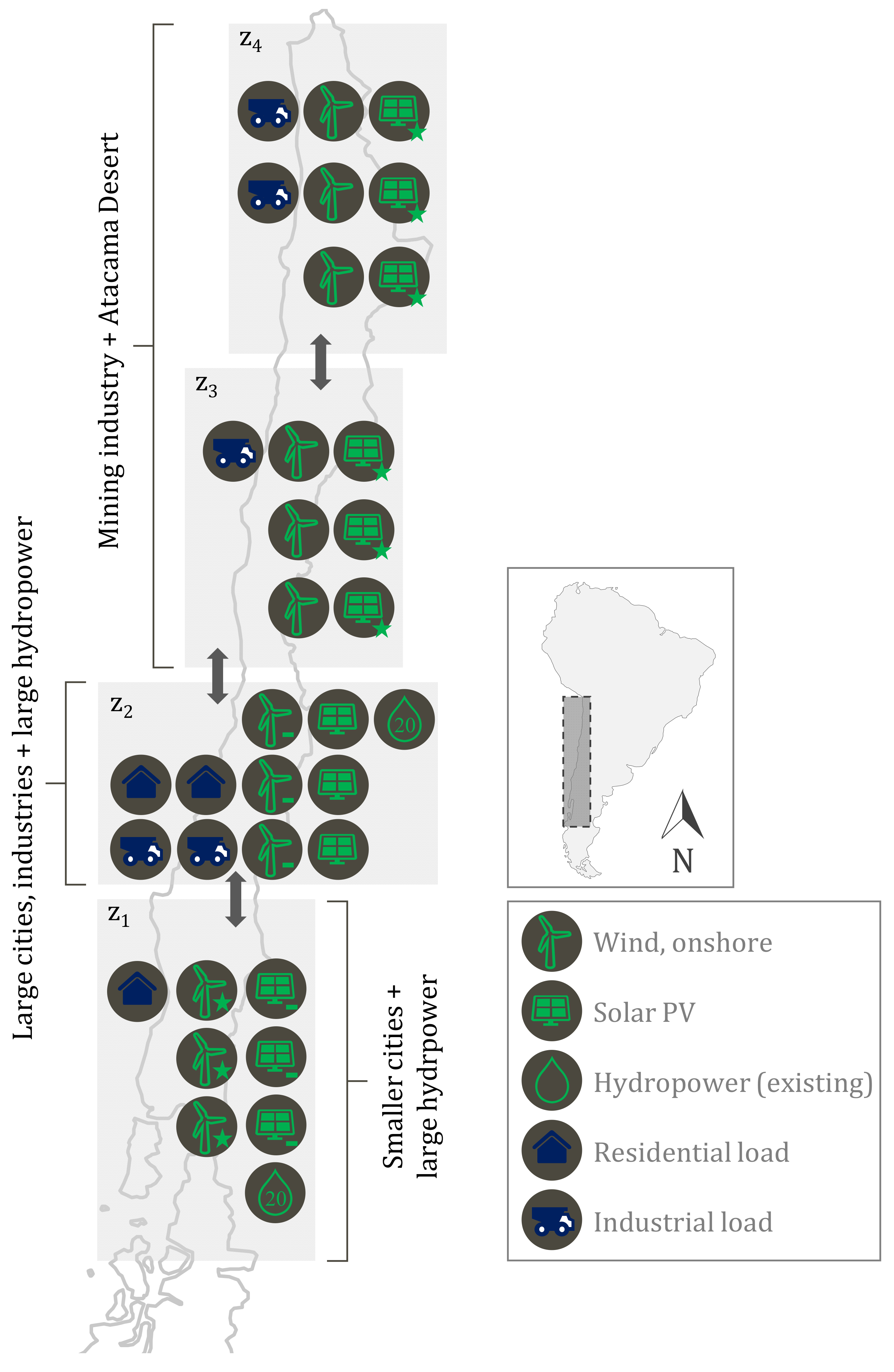
3.1. Description of the Power System

We use a static planning approach with hourly resolution (i.e., 8760 sequential time steps) to design Chile’s power system at the year 2050. We modeled the Chilean power system in four zones (see Figure 1). Each zone includes three profiles for both wind and solar technologies, totalizing 24 profiles and all (existing) hydropower cascades. These profiles were obtained from the tool Solar and Wind Energy Explorer [34,35] and follow the definition used in our previous publication [21]. For each study case, the main outputs include investments in wind and solar photovoltaic power and battery systems.

3.2. Input Data

The main inputs for our planning tool refer to investment costs, technical data for technologies, and profiles for renewable generation. As a summary, Table 1 shows the investment costs and lifetime used for BESSs and RGTs. These data are based on [36], which uses experience curves to project the costs to the year 2050, and have been validated in [37,38]. The yearly load profiles (with hourly resolution) of each zone are based on [39]. These were then projected to the year 2050 using the growth rates given by Chile’s National Energy Commission [40]. This results in an average demand of 3, 12, 2, and 6 GW (23 GW in total) for the zones Z1 to Z4, respectively, and a peak load of 29 GW. All inputs are openly available in [41]. Note that in contrast to that database, in the present study, we did not consider pumped hydro nor hydrogen storage. Furthermore, the data for the stability constraint will be explained in the next subsection.

3.3. Defines Cases and Resulting Scenarios

To evaluate the role that BESSs and RGTs can play in providing FFR in systems with low inertia, we defined three sets of cases to be evaluated in our study: (i) different levels of existing inertia in the system, (ii) different stability constraints (system-wide f -constraint versus zone-specific f -constraints), and (iii) different strategies regarding what technology (renewable and/or storage) is allowed to provide the FFR. These sets are described next and summarized in Table 2.
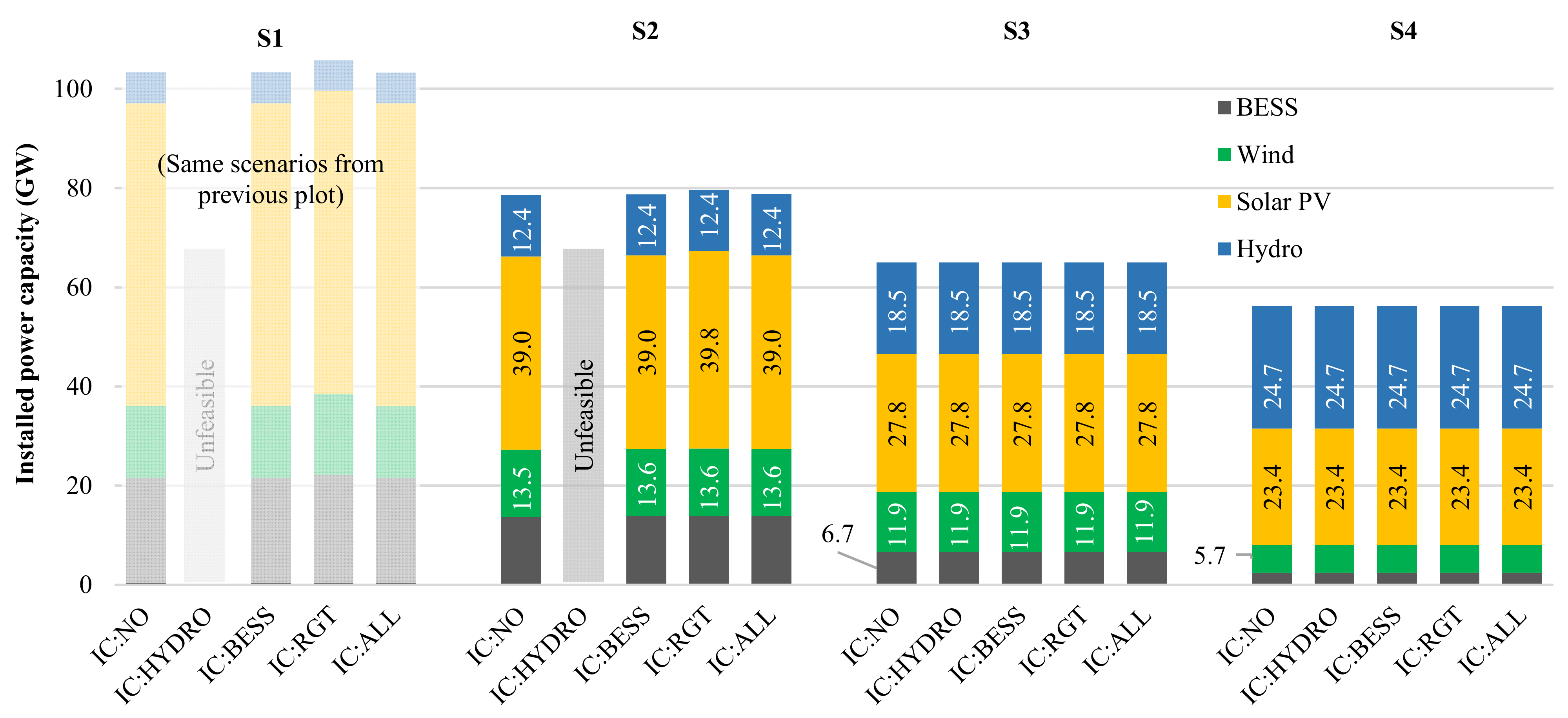
  • Level of available inertia: Regarding possible future levels of system inertia, we built four scenarios by varying the installed capacity of hydropower (denoted S1 to S4). We assumed that according to the decarbonization plan in Chile, rotating masses from fossil generation will not be available in the target year. The first scenario (S1) represents the current situation of hydropower capacities (6 GW) [39]. In each of the following scenarios (S2, S3, S4), we successively increased the installed capacity by 6 GW, resulting in 24 GW for the last scenario (S4). These values may be realized by incorporating new hydropower projects, re-powering and up-powering of existing installations, and new pumped hydro installations. Regardless of the actual hydropower park in the year 2050, these scenarios are helpful to understand the sensitivity of our results in systems with different levels of inertia which, in practice, could also be provided by other technologies, e.g., flywheels.
  • System-wide versus zone-specific f -constraints: We run the GEP model for cases with a system-wide f-constraint (FS-U) and a set of zone-specific f-constraints (FS-M) for ensuring system frequency stability. Both cases are compared to the case without frequency stability constraints (NS). For the system-wide f-constraint, we consider the loss of the largest generation unit, which is a hydropower unit of 0.7 GW. This sudden generation trip would lead to a power mismatch of 0.7 GW. In the zone-specific f -constraints, we consider the loss of the largest generation unit in each zone (see Table A1, Table A2, Table A3 and Table A4 and Figure A1 in the Appendix A for further details). For zones 1 and 2, we considered large hydro units (0.7 and 0.6 GW, respectively), and for zones 3 and 4, a large renewable power park (0.1 GW for each). Note that, in each case, only the trip of one generating unit at a time is considered.
  • What technology provides reserves: Regarding the technology that may contribute with FFR, we considered the following cases: (i) neither BESSs nor RGTs contribute with FFR (IC: HYDRO), in which case the frequency must be maintained solely by hydropower plants; (ii) only BESSs and hydropower plants contribute with FFR (IC: BESS); (iii) only renewable generators and hydropower plants contribute with FFR (IC: RGT); and (iv) BESSs, RGTs, and hydropower plants contribute with FFR (IC: ALL).
Resulting scenarios: Scenario sets (i) and (ii) relate directly to our research questions 1 and 2, while set (iii) is transversal to both research questions. Consistently, we organize our discussion on what technology provides the reserves into two parts. The first part analyses different levels of inertia (set i by set iii, resulting in 20 cases), and the second part focuses on the location requirements of reserves (set ii by set iii, resulting in 8 cases).

4. Results

In this section, we present the results of our case study for the two scenario sets, as defined in the last paragraph of Section 3.3. First, we discuss how planning with frequency stability constraints impacts the overall investment decisions under different levels of available inertia (Section 4.1). Then, we analyze how the spatial inertia distribution in the network impacts the investment decisions. For this, we compare the results obtained from our GEP model using the system-wide f -constraint and the zone-specific f -constraints (Section 4.2).

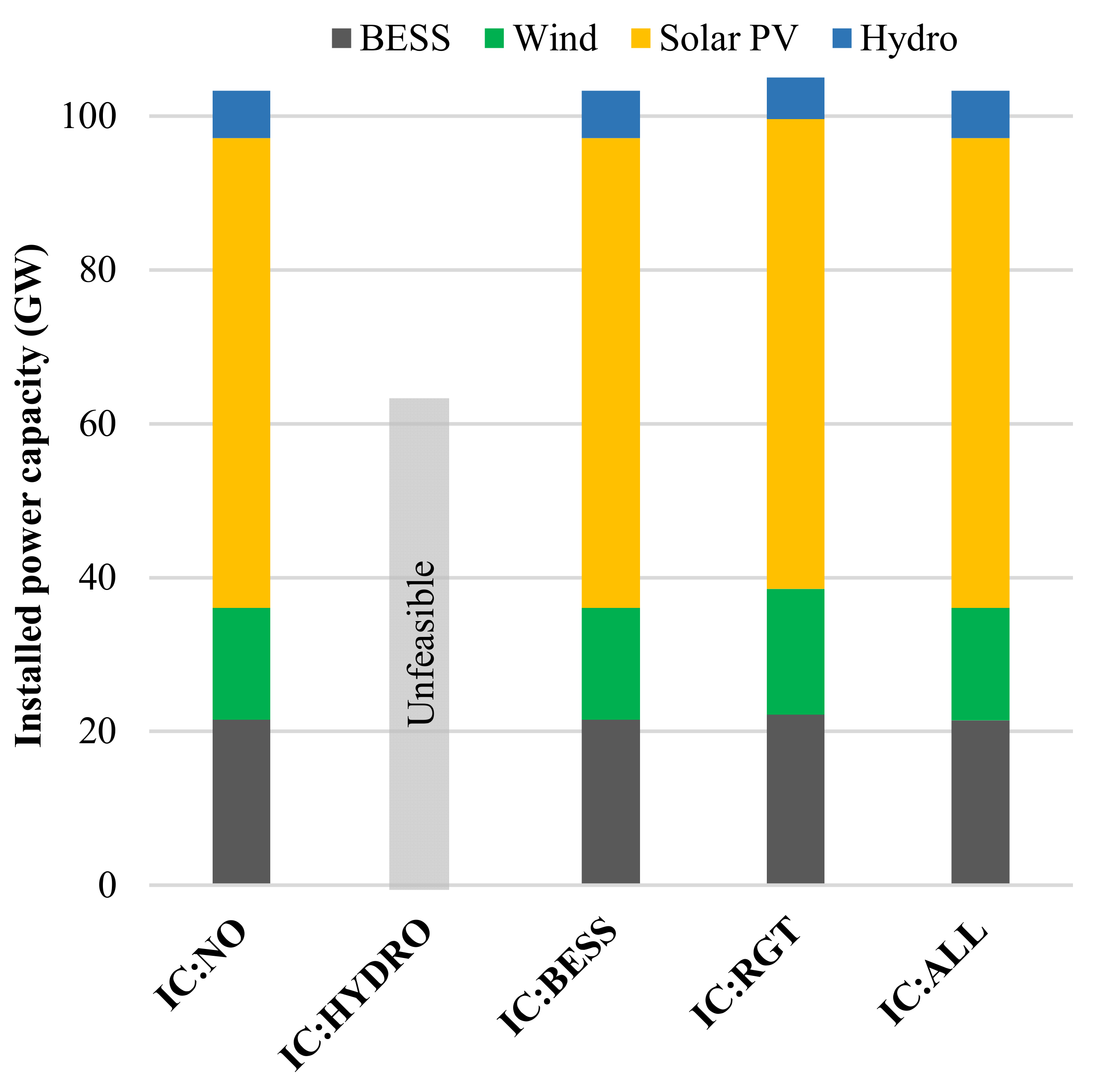
4.1. Impact of Modeling Frequency Constraints on Investment Decisions

In this part, we first analyze how the participation of different technologies in providing FFR impacts the total investment decisions. Then, we inspect these results under scenarios of varying available inertia.
The total (to be) installed capacities of BESS, wind, and solar PV (and hydro, which is constant) of the projected system at the year 2050 are shown in Figure 2. Each bar refers to a case in which a different technology provides FFR. Going from left to right, that is no FFR is modeled, only hydropower provides inertia, only BESS provides FFR, only renewables provide FFR, and all technologies provide FFR (all of these cases correspond to the scenario S1). Figure 2 provides three messages:
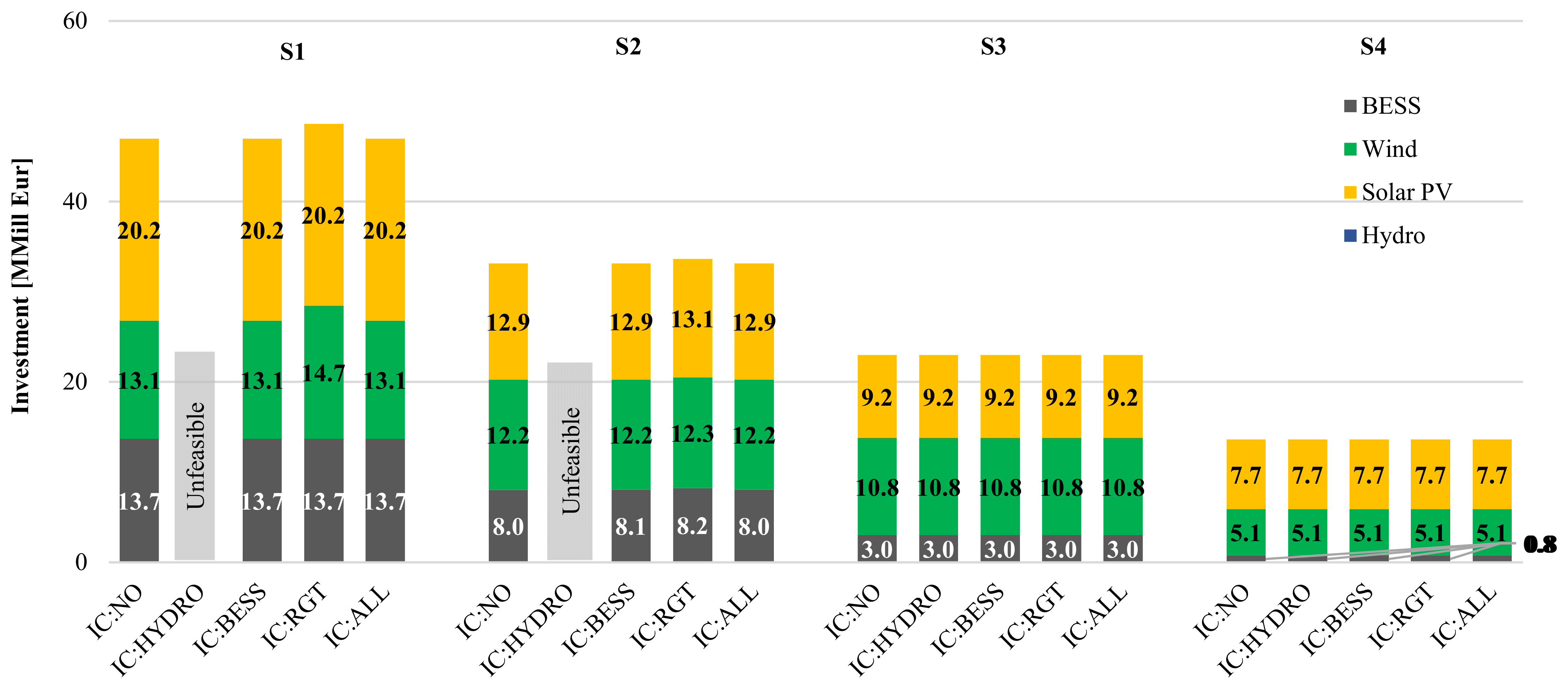
  • Relying solely on hydropower plants to meet the system frequency stability requirements is not sufficient (IC: HYDRO). Here, the planning model is unfeasible. To some extent, this is to be expected, as the frequency requirements are similar to those in the system today, but most of the technologies with rotating masses will have been phased out. If not replaced with new technologies, the system will simply not meet the stability requirements.
  • Exclusively using renewables to contribute with FFR (IC: RGT) is feasible but results in 2–3% larger power capacity investments. The possibility to assure frequency stability only with renewables is an interesting finding, especially if storage technologies happen not to evolve as cheaply as the projections insinuate today. In this context, the ability to offer FFR by RGTs based on adding control loop to the converter controller might be an alternative.
  • When only BESSs aid in FFR provision (IC: BESS), the resulting investment sizes are very similar to the case in which FFR is not modeled (IC: NO). The same holds for the case in which all technologies participate in FFR provision (IC: ALL). This happens due to the topology of the resulting system: solar PV, being the most cost-effective solution (given its cheap costs and Chile’s excellent solar resources), is massively deployed. This, in turn, triggers large investments in batteries for shifting energy from day to night (energy arbitrage). In addition, the inertia requirements (0.7 GW) seem rather small next to the over 20 and 6 GW of power capacity from batteries and hydropower plants, respectively. From these capacities, some might always be readily available to meet other services, such as FFR.
Next, let us take a look at scenarios of different levels of available inertia. Figure 3 shows these scenarios (S1–S4) in four groups. The set of scenarios on the furthest left (S1), are the same results as discussed in Figure 2. One group to the right shows the results for a system with more available inertia (S2) and so on. Here, we observe the following:
  • In S2 (double as much available inertia as S1), when hydropower is the only provider of inertial response (IC: HYDRO), the projected system is unable to comply with the frequency stability constraints without help from BESSs or RGTs. Again, investments are slightly higher if renewables are the only technology allowed to provide FFR (IC: RGT). Moreover, similarly to S1, if batteries (IC: BESS) or all technologies (IC: ALL) participate, the investment recommendations are very similar to the case in which no FFR is prescribed (IC: NO).
  • In scenarios S3 and S4, planning with the frequency stability constraints has negligible effects on the optimal solution. Here, the available inertia is large enough to meet the system’s requirements without the need for further action.
As a concluding remark of Section 4.1, in highly renewable electrical systems, it will be necessary to include FFR from some converter-based technology, as already being discussed in the literature. From a regulatory viewpoint, our results show that requiring FFR from RGTs may not be mandatory as long as that response is provided by BESSs. This may also result in additional savings in the total system costs since RGTs may be deployed without additional equipment (including software for FFR) and without the foregone energy sales (due to de-loaded operation). All these conclusions are robust for different levels of available system inertia, going from the minimum projected level of inertia (S1) up to double that value (S2).

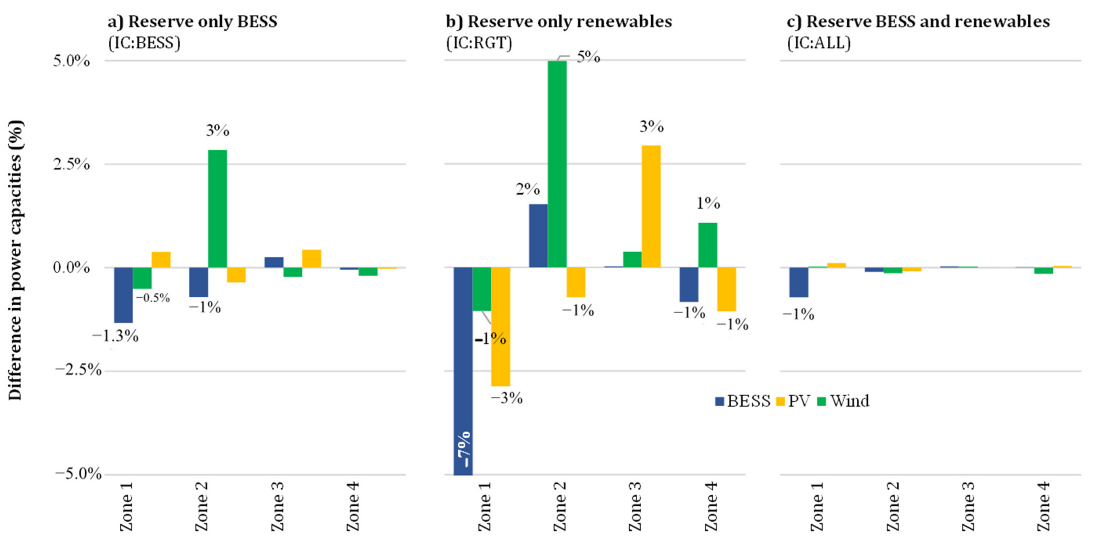
4.2. Impact of Zone-Specific Frequency Constraints on Investment Decisions

In this section, we will study how modeling a system-wide frequency stability constraint is different from a set of zone-specific frequency stability constraints. In particular, we will focus on how these two cases impact (i) the location of investments and (ii) the location of the main FFR providers.
The difference in investments, arising from modeling a system-wide versus a zone-specific f -constraint, is shown in Figure 4. This figure shows how the power capacity of the different technologies (BESS, PV, WIND) is relocated along the four zones of the model. It is organized into three panels: (a) when only BESS provides reserves, (b) when only renewables provide reserves, and (c) when all technologies provide reserves. From panel b (IC: RGT), we can read, for example, how the power capacities from BESS decrease by 7% in zone 1 and increase by 2% in zone 2 when requesting zone-specific reserves. Overall, what we can learn from Figure 4 is the following:
  • There is a measurable relocation of investments. This holds for all technologies, and under all scenarios. In other words, if the spatial inertia distribution in the network is uneven, zone-specific inertia modeling should be preferred. The difference in investment sizes is ranged between −7% and 5%.
  • When comparing the three panels (a, b, c), it becomes clear how the largest difference occurs when only renewables provide FFR. The other extreme is when all technologies participate in reserve provision (panel c), where the relocation of investments is minimum.
  • The largest relocations occur for zone 1 and zone 2. Zone 1 generally shows lower investments and zone 2 higher investments, when using a zone-specific approach. The resulting investments in zones 3 and 4 are more stable.
  • When planning with zone-specific f -constraints, batteries are generally down-sized and compensated by larger wind farms.
  • Finally, when analyzing the (system) total investment sizes (not directly shown here, but computable when summing all the differences), there is no significant difference between the two ways of modeling the frequency constraint. This also holds for total costs.
In terms of which technology provides FFR (and in which zone), Figure 5 provides the overview. It follows the same structure as Figure 4, but instead of showing investments, it shows the (difference in) operational values on who provides the reserves. This figure reveals that when requesting a zone-specific constraint level:
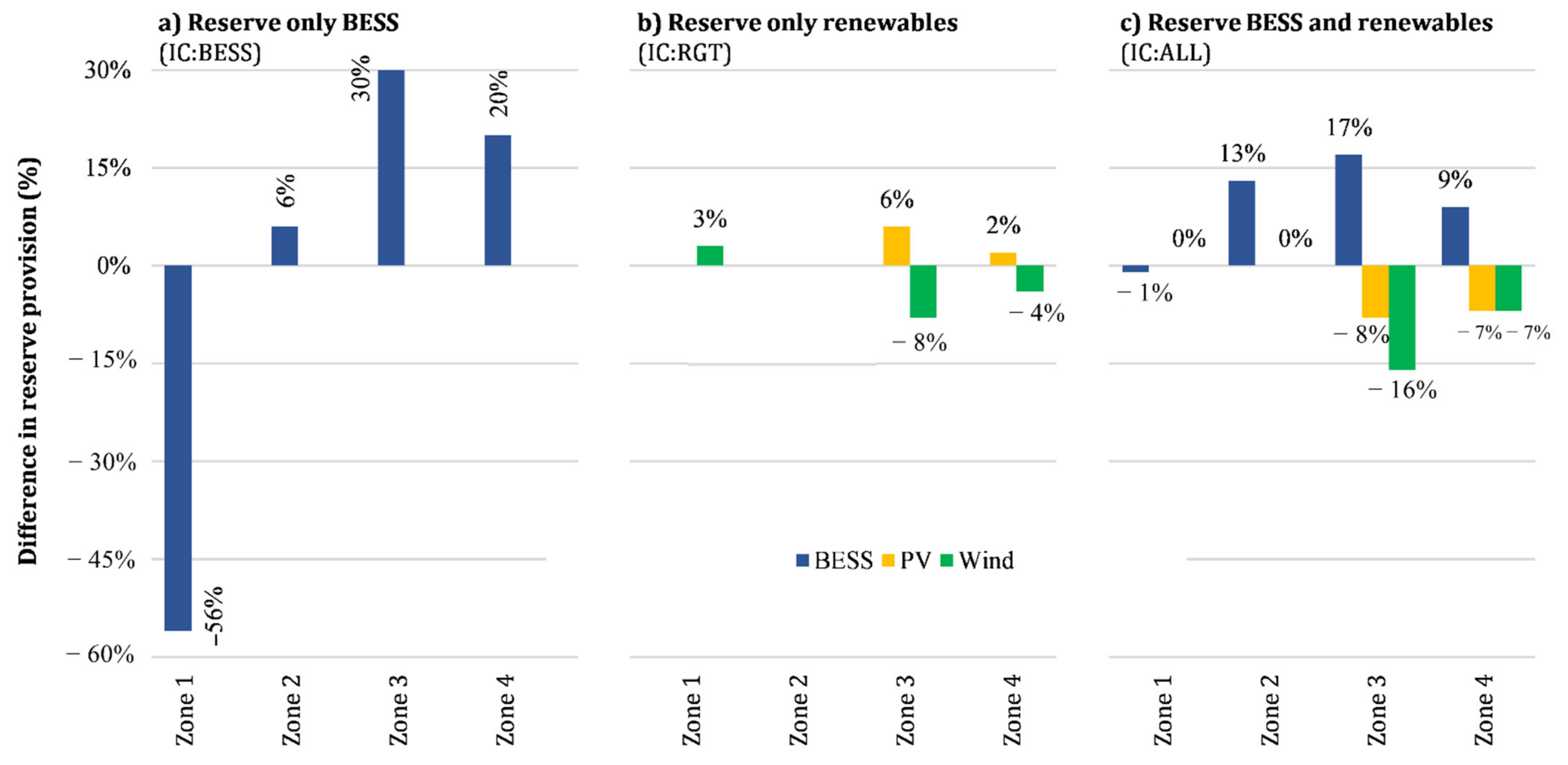
  • There is an impact on the location of the reserve provider. This impact occurs for all scenarios and zones and ranges between −56% and 30% (see Figure 5).
  • The reserve providers suffer from important relocations. The operational difference is particularly large when only batteries offer FFR (panel a), with an average of 30%. On the other hand, when only renewables offer reserves (panel b), that relocation is minimum. The latter can be explained by the slack that the renewable power plants have, given their over-investments which results in energy curtailment when they are the only reserve providers (recall Figure 2).
Summarizing Section 4.2, requesting zone-specific f -constraints (as opposed to a system-wide requirement), might not impact the (system’s) total investments, but it does affect the location of the different technologies up to approximately ±5%. This is especially relevant when finding the precise location is of interest. When taking a look at who provides FFR (and where), there is also an impact on the location. Batteries are particularly strongly affected.

5. Conclusions

In the present work, we studied the impact of requiring FFR on the investment decisions of a future renewable power system. For this purpose, we extended an optimization-based planning tool by adding an equation for inertial frequency response. Then, in a case study, we used different scenarios, varying (i) the reserve provider (batteries, renewable generators, and conventional hydropower), (ii) the available level of reserves (based on defined levels of conventional technologies), and (iii) the requirement of a system-wide versus a zone-specific reserve to study their impact on investment decisions.
We found that in highly renewable power systems, requesting additional technologies to provide FFR will be mandatory. That response could come from renewable generators (by operating them in de-load mode), calling for slight over-investments, but it seems more efficient for batteries to provide such a response. The total power capacities are not strongly impacted because there are large battery systems available in the system, triggered by the need for buffering solar energy. These messages hold for different levels of available inertia.
Modeling zone-specific (versus system-wide) inertia requirements impacts the location of the different technologies up to approximately +5%, although, again, the total capacities remain unaltered. When analyzing what technology provides the reserves and in what zone, there are large differences observed, especially in batteries.
For future work, we envision the need to focus on the pathway toward fully renewable systems because there might be critical points along the way (in terms of critical values of available flexibility and inertia). Furthermore, dynamic system simulation should be performed to validate the found investment size from a stability point of view.
In general, our findings are important for planners, especially when the location of the energy infrastructure is of interest, and for regulators in the task of defining new stability services for future power systems.

Author Contributions

Conceptualization, C.R. (Claudia Rahmann), R.Á. and J.H.; investigation, P.G.-I.; methodology, C.R., R.Á. and J.H.; software, J.H. and P.G.-I.; formal analysis, P.G.-I., C.R. (Claudia Rahmann), R.Á., J.H.; validation, C.R. (Christian Rehtanz) and W.N.; writing—original draft preparation, P.G.-I., C.R. (Claudia Rahmann), R.Á. and J.H.; writing—review and editing, C.R., R.Á., J.H., C.R. (Christian Rehtanz) and W.N. All authors have read and agreed to the published version of the manuscript.

Funding

The authors thank the support of the Chilean National Research and Development Agency (ANID), ANID/Fondap/15110019, ANID/FONDECYT/11160228, ANID/FONDECYT/1201676, and the German Research Foundation (DFG-NO 805/11-1).

Institutional Review Board Statement

Not applicable.

Informed Consent Statement

Not applicable.

Data Availability Statement

Input data can be found on reference [41].

Conflicts of Interest

The authors declare no conflict of interest.

Appendix A

Table A1. Nomenclature of the model: sets.
NameDescription
t Time steps
r Renewable power plants
s Storage technologies
HHydropower plants
p v Photovoltaic plants
WWind plants
z i Zone “i”
Table A2. Nomenclature of the model: Operational variables.
NameUnits Description
p s , t , z c h a r g e  
p s , t , z d i s c h a r g e
MWPower charged to or discharged from storage s in zone z at time t
f R e s t , z , s S MWContingency reserve from storage s in zone z at time t
f R e s t , z , p v P V MWContingency reserve from photovoltaic in zone z at time t
f R e s t , z , w W MWContingency reserve from wind in zone z at time t
f R e s t , z , w R MWContingency reserve from renewables in zone z at time t
H s y s seginertia of the system
Δ P p.u.Power imbalance
Δ P R e n e w a b l e p.u.Power contributions of RGTs
Δ P E S S p.u.Power contributions of BESSs
Δ P i m p   t , z MWImport power per zone z at time t in case of contingency
Δ P exp t , z MWExport power per zone z at time t in case of contingency
P t , r , z MWOffered energy from renewables in zone z at time t
S i MVANominal power of unit t
S b MVACommon system base
s t o r e d s , z , t MWhStored energy of storage s in zone z at time t
Table A3. Nomenclature of the model: investment variables.
NameUnits Description
P r , z i n s MWInstalled power capacity of renewable technology r in zone z
P l i n s MWInstalled power capacity of transmission lines l
P s , z i n s   MWInstalled power capacity (discharging, charging) of storage s in zone z
E s , z i n s MWhInstalled energy capacity of storage s in zone z
Table A4. Nomenclature of the model: inputs.
NameUnits Description
P r o f i l e r , t , z %Profile of renewable source r in zone z at time t
ROCOFHz/segRate of change of frequency
f 0 HzNominal frequency of the system
H i segInertia constant of unit i
H z segAmount of inertia for each zone
Δ P e MWEquivalent power contingency
Figure A1. Investment cost per technology in M Mill: sensitivities to different levels of available inertia.
Sustainability 13 05656 g0a1

References

  1. REN21. Renewables 2018 Global Status Report; REN21: Paris, France, 2018. [Google Scholar]
  2. Bloom, A.; Helman, U.; Holttinen, H.; Summers, K.; Bakke, J.; Brinkman, G.; Lopez, A. It’s Indisputable: Five Facts about Planning and Operating Modern Power Systems. IEEE Power Energy Mag. 2017, 15, 22–30. [Google Scholar] [CrossRef]
  3. Milano, F.; Dorfler, F.; Hug, G.; Hill, D.J.; Verbic, G. Foundations and Challenges of Low-Inertia Systems (Invited Paper). In Proceedings of the 2018 Power Systems Computation Conference (PSCC), Dublin, Ireland, 11–15 June 2018. [Google Scholar]
  4. Tielens, P.; Van Hertem, D. The relevance of inertia in power systems. Renew. Sustain. Energy Rev. 2016, 55, 999–1009. [Google Scholar] [CrossRef]
  5. Kroposki, B.; Johnson, B.; Zhang, Y.; Gevorgian, V.; Denholm, P.; Hodge, B.-M.; Hannegan, B. Achieving a 100% Renewable Grid: Operating Electric Power Systems with Extremely High Levels of Variable Renewable Energy. IEEE Power Energy Mag. 2017, 15, 61–73. [Google Scholar] [CrossRef]
  6. Ulbig, A.; Borsche, T.; Andersson, G. Impact of Low Rotational Inertia on Power System Stability and Operation. IFAC Proc. Vol. 2014, 47, 7290–7297. [Google Scholar] [CrossRef] [Green Version]
  7. IEEE Power & Enery Society. Impact of Inverter Based Generation on Bulk Power System Dynamics and Short-Circuit Performance—PES-TR68; IEEE Power & Enery Society: Piscataway, NJ, USA, 2018; p. 63. [Google Scholar]
  8. Lew, D.; Brinkman, G.; Kumar, N.; Lefton, S.; Jordan, G.; Venkataraman, S. Finding Flexibility: Cycling the Conventional Fleet. IEEE Power Energy Mag. 2013, 11, 20–32. [Google Scholar] [CrossRef]
  9. Etxegarai, A.; Eguia, P.; Torres, E.; Iturregi, A.; Valverde, V. Review of grid connection requirements for generation assets in weak power grids. Renew. Sustain. Energy Rev. 2015, 41, 1501–1514. [Google Scholar] [CrossRef]
  10. Rahmann, C.; Vittal, V.; Ascui, J.; Haas, J. Mitigation Control against Partial Shading Effects in Large-Scale PV Power Plants. IEEE Trans. Sustain. Energy 2015, 7, 173–180. [Google Scholar] [CrossRef]
  11. Rahmann, C.; Mayol, C.; Haas, J. Dynamic control strategy in partially-shaded photovoltaic power plants for improving the frequency of the electricity system. J. Clean. Prod. 2018, 202, 109–119. [Google Scholar] [CrossRef]
  12. Tamrakar, U.; Shrestha, D.; Maharjan, M.; Bhattarai, B.P.; Hansen, T.M.; Tonkoski, R. Virtual Inertia: Current Trends and Future Directions. Appl. Sci. 2017, 7, 654. [Google Scholar] [CrossRef]
  13. Dreidy, M.; Mokhlis, H.; Mekhilef, S. Inertia response and frequency control techniques for renewable energy sources: A review. Renew. Sustain. Energy Rev. 2017, 69, 144–155. [Google Scholar] [CrossRef]
  14. Haas, J.; Cebulla, F.; Cao, K.; Nowak, W.; Palma-Behnke, R.; Rahmann, C.; Mancarella, P. Challenges and trends of energy storage expansion planning for flexibility provision in low-carbon power systems—A review. Renew. Sustain. Energy Rev. 2017, 80, 603–619. [Google Scholar] [CrossRef] [Green Version]
  15. Cebulla, F.; Haas, J.; Eichman, J.; Nowak, W.; Mancarella, P. How much electrical energy storage do we need? A synthesis for the U.S., Europe, and Germany. J. Clean. Prod. 2018, 181, 449–459. [Google Scholar] [CrossRef]
  16. Zerrahn, A.; Schill, W.-P. Long-run power storage requirements for high shares of renewables: Review and a new model. Renew. Sustain. Energy Rev. 2017, 79, 1518–1534. [Google Scholar] [CrossRef]
  17. Hart, E.K.; Jacobson, M.Z. A Monte Carlo approach to generator portfolio planning and carbon emissions assessments of systems with large penetrations of variable renewables. Renew. Energy 2011, 36, 2278–2286. [Google Scholar] [CrossRef]
  18. De Sisternes, F.J.; Jenkins, J.D.; Botterud, A. The value of energy storage in decarbonizing the electricity sector. Appl. Energy 2016, 175, 368–379. [Google Scholar] [CrossRef] [Green Version]
  19. Genoese, F.; Genoese, M. Assessing the value of storage in a future energy system with a high share of renewable electricity generation an agent-based simulation approach with integrated optimization methods. Energy Syst. 2014, 5, 19–44. [Google Scholar] [CrossRef]
  20. Carrion, M.; Dvorkin, Y.; Pandzic, H. Primary Frequency Response in Capacity Expansion with Energy Storage. IEEE Trans. Power Syst. 2018, 33, 1824–1835. [Google Scholar] [CrossRef]
  21. Haas, J.; Cebulla, F.; Nowak, W.; Rahmann, C.; Palma-Behnke, R. A multi-service approach for planning the optimal mix of energy storage technologies in a fully-renewable power supply. Energy Convers. Manag. 2018, 178, 355–368. [Google Scholar] [CrossRef]
  22. Inzunza, A.; Moreno, R.; Bernales, A.; Rudnick, H. CVaR Constrained Planning of Renewable Generation with Consideration of System Inertial Response, Reserve Services and Demand Participation. Energy Econ. 2016, 59, 104–117. [Google Scholar] [CrossRef]
  23. Komasatid, K.; Jiriwibhakorn, S. Flexibility and Frequency Security Enhancement to Generation Expansion Planning Framework. In Proceedings of the 2019 IEEE PES GTD Grand International Conference and Exposition Asia (GTD Asia), Bangkok, Thailand, 19–23 March 2019; pp. 762–767. [Google Scholar]
  24. Chavez, H.; Baldick, R.; Sharma, S. Governor Rate-Constrained OPF for Primary Frequency Control Adequacy. IEEE Trans. Power Syst. 2014, 29, 1473–1480. [Google Scholar] [CrossRef]
  25. Haas, J.; Nowak, W.; Palma-Behnke, R. Multi-objective planning of energy storage technologies for a fully renewable system: Implications for the main stakeholders in Chile. Energy Policy 2019, 126, 494–506. [Google Scholar] [CrossRef]
  26. GAMS Development Corp. GAMS-Cutting Edge Modeling; GAMS Development Corp.: Fairfax, VA, USA, 2018. [Google Scholar]
  27. IBM. IBM ILOG CPLEX Optimization Studio; IBM: Armonk, NY, USA, 2018. [Google Scholar]
  28. Ahmadi, H.; Ghasemi, H. Security-Constrained Unit Commitment with Linearized System Frequency Limit Constraints. IEEE Trans. Power Syst. 2014, 29, 1536–1545. [Google Scholar] [CrossRef]
  29. Egido, I.; Fernandez-Bernal, F.; Centeno, P.; Rouco, L. Maximum Frequency Deviation Calculation in Small Isolated Power Systems. IEEE Trans. Power Syst. 2009, 24, 1731–1738. [Google Scholar] [CrossRef]
  30. Rahmann, C.; Chamas, S.I.; Alvarez, R.; Chavez, H.; Ortiz-Villalba, D.; Shklyarskiy, Y. Methodological Approach for Defining Frequency Related Grid Requirements in Low-Carbon Power Systems. IEEE Access 2020, 8, 161929–161942. [Google Scholar] [CrossRef]
  31. Bomer, J.; Burges, K.; Nabe, C.; Poller, M. All Island TSO Facilitation of Renewables Studies; EirGrid: Dublin, Ireland, 2010; pp. 1–107. [Google Scholar]
  32. Hung, W.; Ray, G.; Stein, G. Frequency Changes during Large Disturbances WG; National Grid plc: London, UK, 2010. [Google Scholar]
  33. Ahmadyar, A.S.; Riaz, S.; Verbic, G.; Riesz, J.; Chapman, A. Assessment of minimum inertia requirement for system frequency stability. In Proceedings of the 2016 IEEE International Conference on Power System Technology (POWERCON), Wollongong, Australia, 28 September–1 October 2016; pp. 1–6. [Google Scholar]
  34. Molina, A.; Falvey, M.; Rondanelli, R. A solar radiation database for Chile. Sci. Rep. 2017, 7, 1–11. [Google Scholar] [CrossRef] [PubMed]
  35. Department of Geophysics, University of Chile and Ministry of Energy of Chile. Explorador de Energía Solar (Solar Energy Explorer). 2012. Available online: http://walker.dgf.uchile.cl/Explorador/Solar2/ (accessed on 25 August 2015).
  36. Child, M.; Breyer, C.; Bogdanov, D.; Fell, H.-J. The role of storage technologies for the transition to a 100% renewable energy system in Ukraine. Energy Proc. 2017, 135, 410–423. [Google Scholar] [CrossRef]
  37. Kilickaplan, A.; Bogdanov, D.; Peker, O.; Caldera, U.; Aghahosseini, A.; Breyer, C. An energy transition pathway for Turkey to achieve 100% renewable energy powered electricity, desalination and non-energetic industrial gas demand sectors by 2050. Sol. Energy 2017, 158, 218–235. [Google Scholar] [CrossRef]
  38. Breyer, C.; Afanasyeva, S.; Brakemeier, D.; Engelhard, M.; Giuliano, S.; Puppe, M.; Schenk, H.; Hirsch, T.; Moser, M. Assessment of mid-term growth assumptions and learning rates for comparative studies of CSP and hybrid PV-battery power plants. AIP Conf. Proc. 2017, 1850. [Google Scholar] [CrossRef] [Green Version]
  39. Alvarez, R.; Moser, A.; Rahmann, C.A. Novel Methodology for Selecting Representative Operating Points for the TNEP. IEEE Trans. Power Syst. 2016, 32, 2234–2242. [Google Scholar] [CrossRef]
  40. National Energy Commission of Chile (CNE). Electricity Tariffing. 2013. Available online: http://www.cne.cl/tarificacion/electricidad/introduccion-a-electricidad (accessed on 29 August 2013).
  41. Haas, J. Inputs for LEELO (Long-Term Energy Expansion Linear Optimization) (Version v38/v39) [Data Set]; Zenodo: Meyrin, Switzerland; Available online: https://zenodo.org/record/1344412#.YIv__rWGmHs (accessed on 3 May 2018).
Figure 1. Diagram of the Chilean power system divided in four zones [25].
Sustainability 13 05656 g001
Figure 2. Impact of planning with frequency stability constraints on installed power capacities which offer the FFR.
Sustainability 13 05656 g002
Figure 3. Impact of planning with frequency stability on installed power capacities: sensitivities to different levels of available inertia.
Sustainability 13 05656 g003
Figure 4. Relocation of investments depending on what technology provides virtual inertia. Negligible values are omitted for clarity purposes.
Sustainability 13 05656 g004
Figure 5. Relocation of reserves depending on what technology provides FFR. Negligible values are omitted for clarity purposes.
Sustainability 13 05656 g005
Table 1. Costs and lifetime used for BESS and RGTs.
TechnologyInvestment Costs Lifetime
[Years]
Wind900 k€/MW25
PV330 k€/MW40
BESS24.9/70.9 k€/MWh10
Table 2. List of defined cases and abbreviations.
Set of CasesCodeDescription
Levels of available inertiaS16 GW
S212 GW
S318 GW
S424 GW
System-wide versus zone-specific reservesSWSystem-wide frequency stability constraint
ZSZone-specific frequency stability constraint
What technology provides reserves (FFR contribution)IC: NOWithout frequency stability constraint
IC: HYDROOnly hydropower provides FFR
IC: BESSOnly BESSs and hydropower plants provide FFR
IC: RGTOnly RGTs and hydropower plants provide FFR
IC: ALLBESSs, RGTs, and hydropower plants provide FFR
Publisher’s Note: MDPI stays neutral with regard to jurisdictional claims in published maps and institutional affiliations.

