Active and Reactive Power Collaborative Optimization for Active Distribution Networks Considering Bi-Directional V2G Behavior

Abstract

Due to their great potential for energy conservation and emission reduction, electric vehicles (EVs) have attracted the attention of governments around the world and become more popular. However, the high penetration rate of EVs has brought great challenges to the operation of the Active Distribution Network (ADN). On the other hand, EVs will be equipped with more intelligent chargers in the future, which supports the EVs’ high flexibility in both active and reactive power control. In this paper, a distributed optimization model of ADN is proposed by employing the collaborative active and reactive power control capability of EVs. Firstly, the preference of EV users is taken into account and the charging mode of EVs is divided into three categories: rated power charging, non-discharging, and flexible charging–discharging. Then, the reactive power compensation capacity of the plugged-in EV is deduced based on the circuit topology of the intelligent charger and the active–reactive power control model of the EV is established subsequently. Secondly, considering the operation constraints of ADN and the charging–discharging constraints of EVs over the operation planning horizon, the optimization objective of the model is proposed, which consists of two parts: “minimizing energy cost” and “improving voltage profile”. Finally, a distributed solution method is proposed based on the Alternating Direction Method of Multipliers (ADMM). The proposed model is implemented on a 33-bus ADN. The obtained results demonstrate that it is beneficial to achieve lower energy cost and increase the voltage profile of the ADN. In addition, the energy demand of EV batteries in their plugin intervals is met, and the demand preference of EV users is guaranteed.

1. Introduction

With the integration of a large number of distributed generations (DGs), the traditional distribution network (DN) has gradually been transformed to the Active Distribution Network (ADN) [1], which includes many controllable resources. Another aspect worthy of attention is that the large-scale penetration of electric vehicles (EVs) poses new challenges to the operation of ADN. It is anticipated that by 2050, about one hundred million EVs will be produced annually [2]. ADN improves the flexibility and controllability of the DN, and also brings new problems, the most prominent of which is the abnormal voltage fluctuation and congestion in feeders. Due to the development of V2G technology, the bi-directional charging topology capable of four-quadrant operation is gradually becoming the mainstream topology of charging stations [3]. Based on the gradual maturation of V2G technology, coordinating the active and reactive power of EVs has great potential for easing the abnormal fluctuations and feeder congestion of the ADN [4].

One of the distinguishing features of the ADN is that the ADN operator (ADNO) and users can communicate bi-directionally, guaranteed by the strong communication infrastructure [5]. Accordingly, based on the existence of such bi-directional communication systems, there are numerous studies regarding EV management. Abessi et al. [6] improve the resilience of the ADN by optimizing the charging and discharging process of EVs. Wu et al. [7] establish the power optimal allocation strategy of EVs based on the optimization framework of multi-time scale energy management. Shi et al. [8] propose a collaborative optimization model of EV coupled with renewable energy. Meesenburg et al. [9] and Dong et al. [10] manage the charging and discharging process of EVs from the perspective of frequency regulation. All these relevant articles merely focus on the active power management of EVs.

In order to further expand the potentiality of EVs to participate in ADN, this paper not only focuses on the optimization of active power, but also deeply explores the potentiality of EVs in reactive power compensation. In practice, EV is plugged into ADN through the electronic-based converter interface. Pirouzi et al. [11] show that these devices can achieve reactive power management and control with little cost. Reactive power is very important for ADN operation. Currently, reactive power compensation devices for the ADN mainly include the shunt capacitor (SC), static VAR compensator (SVC), and so on. Reactive power compensation devices have higher investment costs. By employing EVs, reactive power compensation based on V2G technology can not only reduce the investment cost of reactive power compensation devices, but also stabilize the bus voltage of the ADN [12]. Fu et al. [13] propose a coordinated EV charging strategy in an unbalanced DN with the support of reactive discharging and phase switching. Saffari et al. [14] propose an integrated framework for the coordinated optimization of the interdependent microgrid (MG) by considering the active–reactive power management of EVs. However, the preference of EV users is ignored. Sousa et al. [15], aiming at the problem that the rapid charging of EVs leads to a drop in voltage, extend a centralized control framework to control the voltage level. However, the coupling between active and reactive power of the EV is ignored, and the preference of users is also not taken into account.

From the point of view of the solution method, the relevant research could be categorized into two general groups: centralized operation [16] and decentralized operation [17]. For the centralized operation, it would be technically intractable for ADNO to directly control the charging–discharging strategy of every EV when a large number of EVs are plugged into the ADN. In addition, the direct connection between the ADN and each EV causes a huge burden on the communication network. However, the significant advantage of the centralized approach is that the centralized algorithm is more suitable for considering ADN constraints (such as power flow, transformer load and other constraints). The decentralized method can deal with larger-scale EVs, but with the typical distributed algorithm, it is not easy to consider the ADN constraints, which will produce negative effects to the optimization process. To cope with the mentioned challenges, a new entity, the EV aggregator (EVA), is introduced to the ADN [18]. From the perspective of ADNO, EVA can be used as a fully controllable resource (this is also convenient for considering grid constraints) [19], and each EVA can independently optimize the process of EVs under its jurisdiction.

According to analysis of existing research, it can be understood that decentralized operation can cope with larger-scale EVs and the optimal management of EVs can improve the safety of the ADN significantly. To summarize the existing literature, most studies on EVs focus only on active power, and a few studies consider the reactive power of EVs. However, as far as the author knows, whether the reactive power of EVs is taken into account or not, there is a unified model for all plugged-in EVs and only the constraints of the charging station and network constraints of ADN are considered in the optimization process. The existing research has obvious limitations and inevitable contradiction with the practical application. These contradictions are mainly reflected in the following aspects:

(1)

In practice, driving is the primary attribute of EVs. As highly autonomous individuals, the preferences of EV users cannot be ignored.

(2)

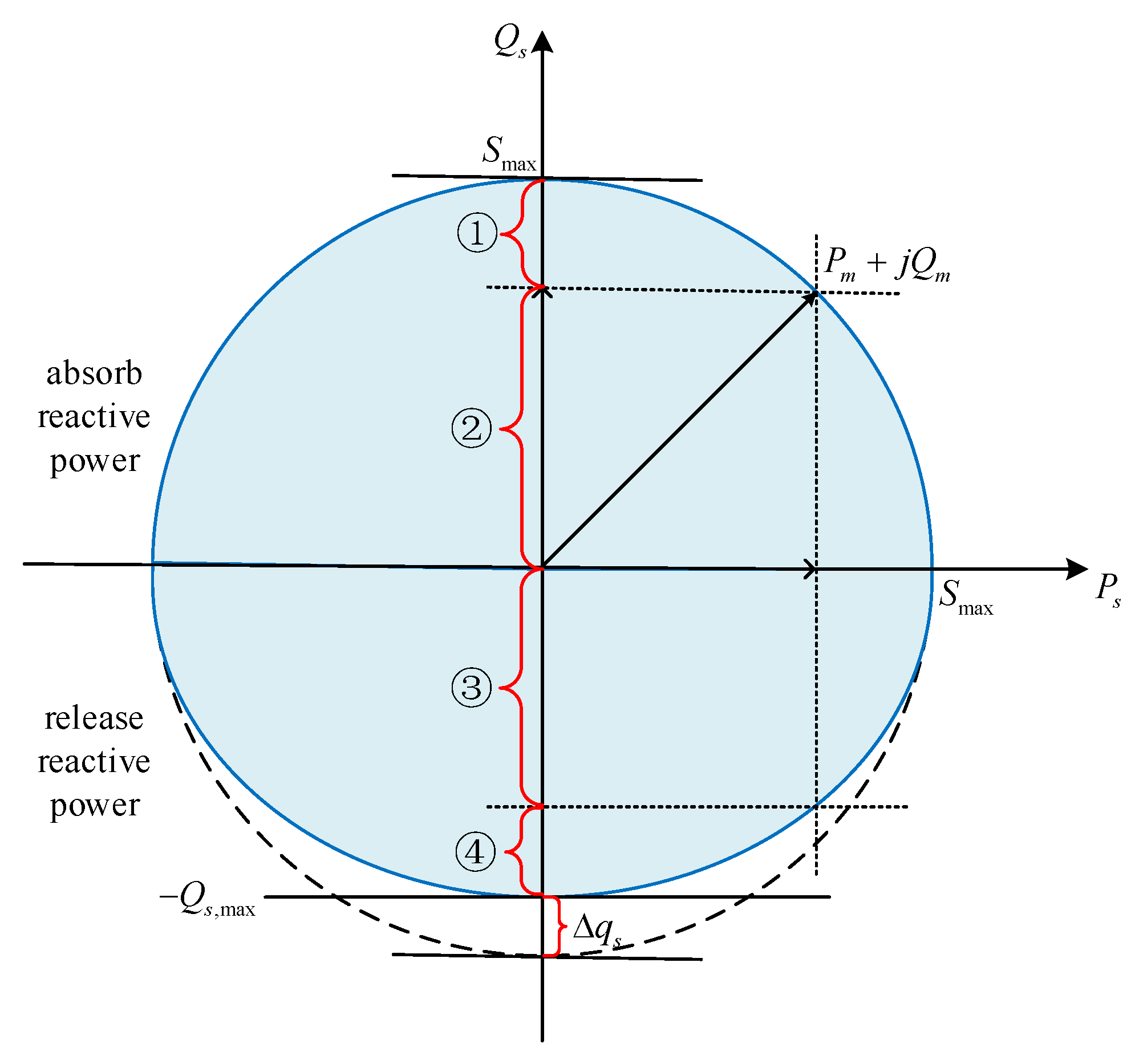
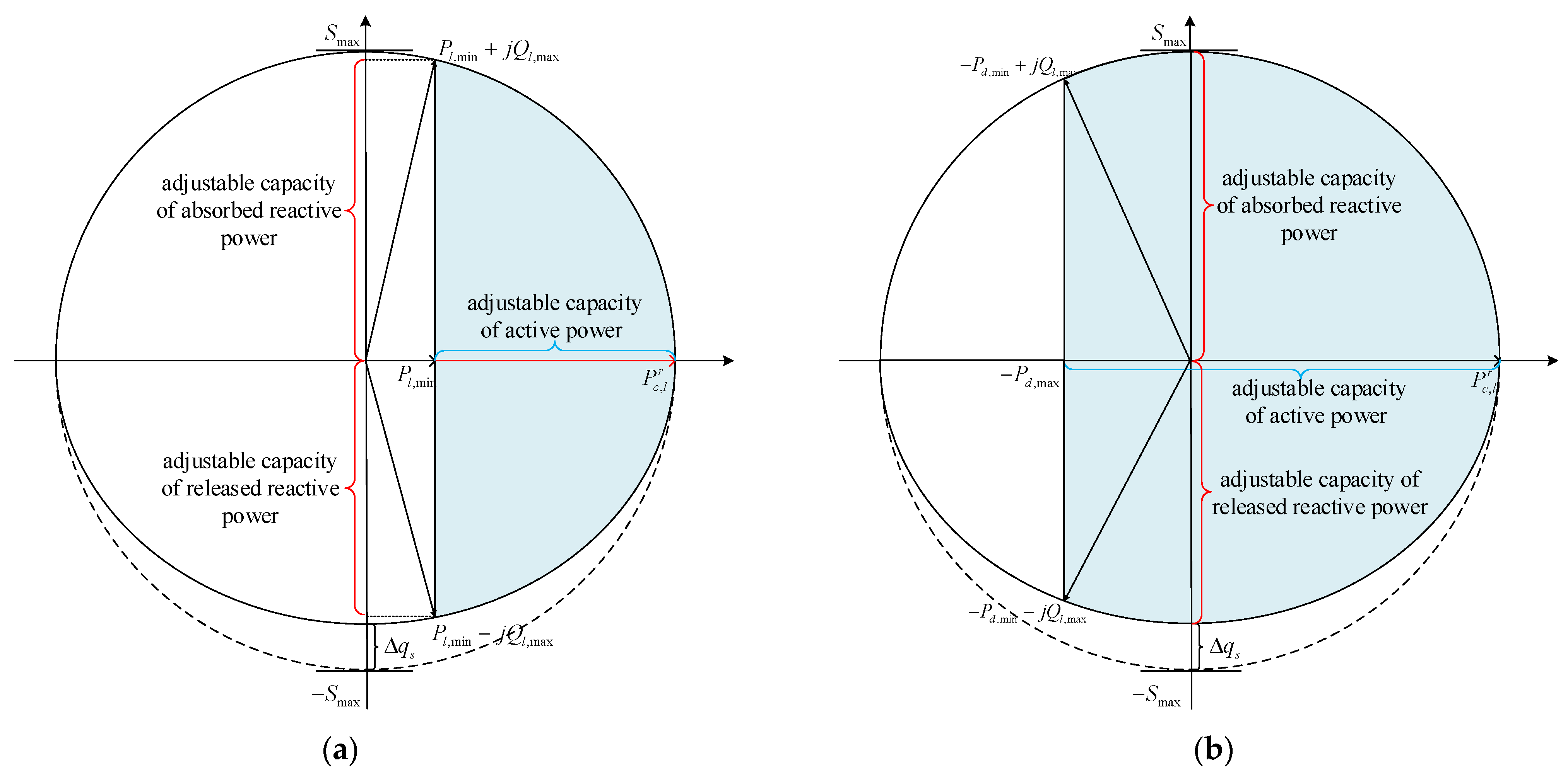
The reactive power compensation capability of EVs is not only restricted by the active power and capacity of the charger, but also needs to consider the constraints of the power electronic equipment of the charger.

(3)

Most of the existing studies are based on the general DN, but ADN contains many DGs, wind power, photovoltaic, reactive power compensation devices, etc., and when the scale of plugged-in EVs and the demand preference of EV users are taken into account, the current research findings are inevitably not applicable to this new scenario.

In this paper, we propose a novel decentralized framework for collaborative optimization of active and reactive power in the ADN with the participation of the EVA. dThe simplified framework is depicted in Figure 1.

We assume that the EVA is allowed to obtain EVs’ behavioral characteristics, including battery parameters (initial SOC, rated charging power, and rated discharging power) and plug-in and plug-out time. EV users determine the charging mode by interacting with the EVA according to their preference. Afterward, the EVA determines the adjustment range of active and reactive power, according to users’ demands. From the point of view of the ADN, the EVA is also a controllable and flexible resource. The ADNO takes the minimum energy cost and the minimum deviation of the voltage amplitude as the goal to coordinate the active and reactive power of EVA under relevant constraints. The main contributions of this paper can be summarized as follows:

(1)

Considering the users’ preference, the plugged-in EVs are subdivided into three categories, and then the EV control model is established separately. The establishment of the differentiated EV control model is more in line with the actual scenario.

(2)

Based on the topological constraints of the charging pile, the reactive power compensation capacity of the EV is modeled to derive a more accurate range of reactive power.

(3)

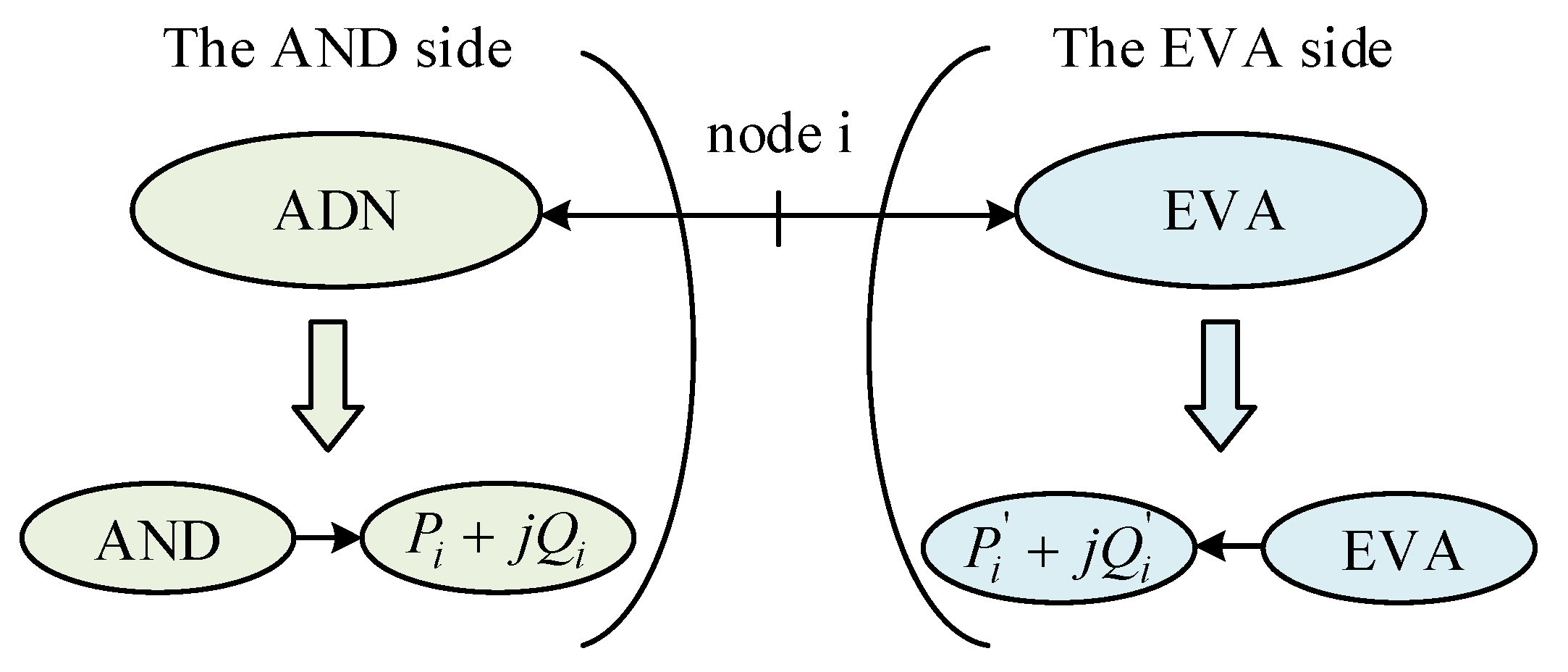
The proposed model is solved by a decentralized algorithm, which is developed based on the Alternating Direction Method of Multipliers (ADMM). The operating problems of the ADNO and EVA are coordinated and optimized independently.

2. Proposed Methodology

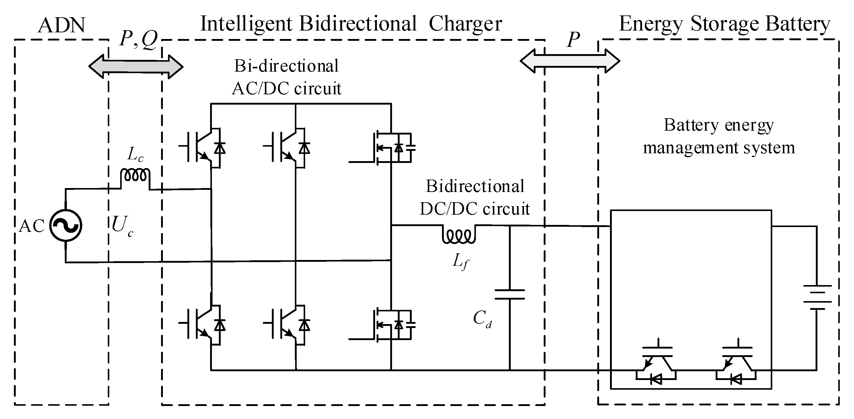
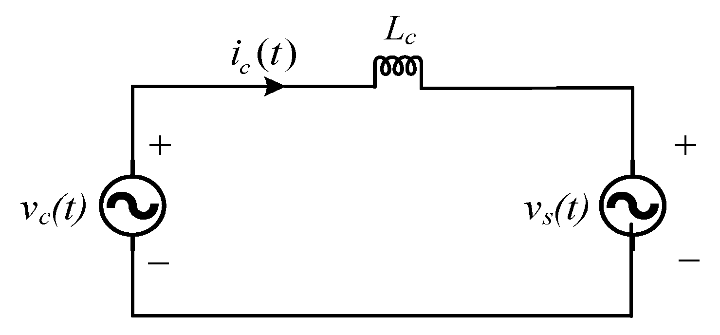
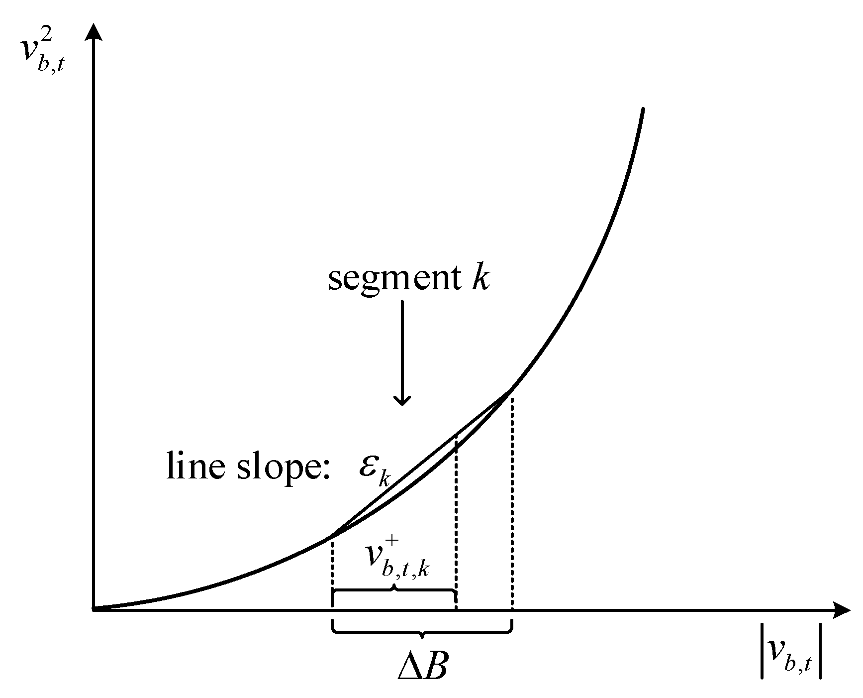
2.1. Modeling Collaborative Active-Reactive Power of EV Cluster

Firstly, we define that the EVs belonging to the same EVA are an EV cluster (EVC). The number of EVC is the same as that of EVA. In this section, the active–reactive power model of a single EV is firstly established, and then the active–reactive power model of each EVC is proposed.

In order to obtain the active–reactive power control model of a single EV, the active power control and reactive power control of a single EV are discussed, respectively, and then the collaborative active–reactive power model is established.

The preference of the EV user is mainly reflected in the difference in the active power. According to the charging or discharging state of the EV battery, the plugged-in EVs are divided into three categories: rated power charging EVs, non-discharging EVs, and flexible charging–discharging EVs. Three different categories reflect the preference of EV users: when the user selects the rated power charging mode, the user expects to minimize the time cost; when the non-discharging mode is selected, it indicates that the user expects to reduce the cost of money without increasing extra battery loss; and when the flexible charging–discharging mode is selected, it means that the user expects the money cost to be minimized. In practice, the user can interact with EVA to determine the charging mode when the EV is plugged into the ADN. The number of EVA in the ADN is denoted as N_A, and D_i,j (i = 1, 2, 3; j = 1, 2, 3…N_A) represents the set of EVs belonging to the ith category in the jth EVA.

The three categories of plugged-in EVs are modeled separately as follows:

$\forall l\in D_{1,j}(j=1,2,\cdots ,N_A)$, the control model of l is formulated by Equations (1) and (2):

$$\left\{\begin{array}{l}{P}_{l,t}=\min (P_{cha},P_{c,l}^r), t\in t_{l,in} and S_{l,t}\in [S_{l,or},S_{l,ex})\\ 0\le P_{l,t}\le \min (P_{cha},P_{c,l}^r), S_{l,t}\ge S_{l,ex}\\ P_{l,t}=0\hspace{1em}, t\notin t_{l,in}\end{array}\right.$$

(1)

$$S_{l,t}=S_{l,or}+{\displaystyle \sum {\eta }_{c,l}·P_{c,l}^r}·\Delta t/E_l$$

(2)

where $P_{cha}$, $P_{c,l}^r$, ${\eta }_{c,l}$, $S_{l,or}$, $S_{l,ex}$ and $E_l$ are the maximum active power, rated charging power, charging efficiency, initial state of charge (SOC), expected SOC of departure and maximum capacity of the battery, respectively. $P_{l,t}$ and $S_{l,t}$ are the actual power and actual SOC of l at timeslot t. $t_{l,in}$ is the time span of the arrival time to departure time of l and $\Delta t$ is the unit interval.

$\forall l\in D_{2,j}(j=1,2,\cdots ,N_A)$, the control model of l is formulated by Equations (3) and (4):

$$\left\{\begin{array}{l}0\le P_{l,t}\le \min (P_{cha},P_{c,l}^r), t\in t_{l,in}\\ P_{l,t}=0\hspace{1em},t\notin t_{l,in}\end{array}\right.$$

(3)

$$S_{l,t}=S_{l,in}+{\displaystyle \sum {\eta }_{c,l}·P_{l,t}}·\Delta t/E_l$$

(4)

$\forall l\in D_{3,j}(j=1,2,\cdots ,N_A)$, the control model of l is formulated by Equations (5) and (6):

$$\left\{\begin{array}{l}-P_{d,l}^r\le P_{l,t}\le \min (P_{cha},P_{c,l}^r), t\in t_{l,in}\\ P_{l,t}=0,t\notin t_{l,in}\\ S_{l,t}\ge S_{l,thr}, P_{l,t}<0\end{array}\right.$$

(5)

$$\left\{\begin{array}{l}{S}_{l,t}=S_{l,t-1}+{\eta }_{c,l}·P_{l,t}·\Delta t/E_l, P_{l,t}\ge 0\\ S_{l,t}=S_{l,t-1}+P_{l,t}·\Delta t/({\eta }_{d,l}·E_l), P_{l,t}<0\end{array}\right.$$

(6)

where $P_{d,l}^r$, ${\eta }_{d,l}$ and $S_{l,thr}$ are the rated discharging power, discharging efficiency and discharging threshold of SOC.

The reactive power operation of the EV is based on the smart charging pile, which has gradually become the focus of attention because of its capability for four-quadrant operation [20]. The representative topology is shown in Figure 2.

As illustrated in Figure 2, the intelligent charger enables a bi-directional flow of active and reactive power between the ADN and EV charger. However, there is only bi-directional active power between the battery and EV charger, which means that the reactive power operation will not affect the battery lifetime.

For the convenience of analysis, the following reasonable assumptions are made:

(1)

The ADN voltage is an ideal sine wave with stable frequency (f = 50 Hz).

(2)

The charger is normally connected to the ADN via cable, so to simplify the calculation, assume that the impedance between the intelligent bi-directional charger and the ADN is the inductive impedance; the sum of the impedance stacks is recorded as L_c.

(3)

The power operation of the charger is realized through the smart control circuit of the charger. The influence of the control circuit on the voltage of the charger is ignored.

Based on the above assumptions, the simplified circuit diagram is shown in Figure 3.

Assume that the grid voltage $u_c(t)$ is $\sqrt{2}\sin (\omega t)$, where $V_c$ is the effective value. Let $\delta$ be the angle that the phase angle of the charger voltage $u_s(t)$ lags the $u_c(t)$; then, $u_s(t)$ can be represented by Equation (7):

$$u_s(t)=\sqrt{2}{V}_s\sin (\omega t-\delta )$$

(7)

The instantaneous power $P_s(t)$ of the charger can be derived:

$$P_s(t)=V_c{I}_c\cos (\theta )-V_c{I}_c\cos (2\omega t-\theta )-\omega L_c{I}_c^2\sin (2\omega t-\theta )$$

(8)

$$\theta ={\tan }^{-1}[\frac{V_c-V_s\cos (\delta )}{V_s\sin (\delta )}]$$

(9)

where $I_c$ is the effective value of the current. Equation (8) shows that the injected instantaneous power of the charger includes two parts: average power and ripple power. The average power is an active power used to charge or discharge the battery of EV, and the ripple power is a kind of oscillating power flowing between the charger and ADN, which is only temporarily stored in the capacitance of the charger. Obviously, the ripple power can characterize the charger’s capacity for reactive power. Through mathematical deduction (the detailed deduction process is given in Appendix A), the maximum reactive power of the charger can be obtained:

$$Q_{s,\max }=\frac{V_c^2·(\sqrt{1+4\frac{\omega L_c}{V_c^2}{S}_{\max }}-1)}{2\omega L_c}$$

(10)

Meanwhile, the power of the charger can satisfy the constraints of Equations (11) and (12):

$$P_s^2+Q_s^2=S^2\le S_{\max }^2,\hspace{1em}when Q_s\ge 0$$

(11)

$$S(1-\frac{\omega L_c}{V_c}·Q_s)\le S_{\max },\hspace{1em}when Q_s<0$$

(12)

The constraints of Equations (11) and (12) show that the reactive operation of the charger is not symmetrical. The limit field of the active and reactive operation of the charger is shown in Figure 4.

The shaded area enclosed by the blue solid line in Figure 4 is the active and reactive operation domain of the charger. The labels ①, ②, ③ and ④ represent the extra absorbable reactive capacity, absorbed reactive capacity, released reactive capacity and extra releasable reactive capacity when P_s = P_m, respectively. It is worth noting that the operation domain is in ideal conditions. When the charger provides extra absorbable or releasable reactive power (e.g., ① or ④), its active power is reduced to zero. In practice, the active power of some EVs is prohibited from being reduced to zero due to the preference of users and the energy demand of the EV battery.

We assume that $P_{cha}$ is equal to $P_{c,l}^r$ in this paper. The active–reactive operation domain of EV, considering the preference of the user and the energy demand of the EV battery, is shown in Figure 5.

$P_{l,\max }$, $-P_{d,\max }$ are the minimum charging and maximum discharging active power when considering the preference of the user and the energy demand of the battery; $Q_{l,\max }$ is the corresponding maximum reactive power. For any EV in $D_{1,j}$ set, Equation (1) indicates that there is no reactive power release or absorption when $S_{l,t}<S_{l,ex}$. The charging power can be cut down when $S_{l,t}\ge S_{l,ex}$. In other words, the EV in $D_{1,j}$ set is equivalent to the EV in $D_{2,j}$ set when $S_{l,t}\ge S_{l,ex}$.

So, the maximum reactive power of the jth (j = 1, 2, …, N_A) EVA can be calculated by Equation (13):

$$\left\{\begin{array}{l}{Q}_{es,abs}^j(t)={\displaystyle \sum _{i=1}^{N_t^j}\sqrt{S_{\max }^2-{(P_{i,t}^j)}^2}}+N_{d,t}^j{S}_{\max }\\ Q_{es,rel}^j(t)={\displaystyle \sum _{i=1}^{N_t^j}(\sqrt{S_{\max }^2-{(P_{i,t}^j)}^2}}-\Delta q_s)+N_{d,t}^j(S_{\max }-\Delta q_s)\\ N_t^j=N_{l,t}^j+N_{2,t}^j+N_{c,t}^j\\ N_{3,t}^j=N_{c,t}^j+N_{d,t}^j\end{array}\right.$$

(13)

where $Q_{es,abs}^j(t)$ and $Q_{es,rel}^j(t)$ are the maximum absorbable reactive power and the maximum releasable reactive power of the jth (j = 1, 2, 3…N_A) EVA at timeslot t, respectively. $N_{l,t}^j$ is the EV number in $D_{1,j}$ set whose SOC has exceeded the value of $S_{l,ex}$ at timeslot t. $N_{2,t}^j$ and $N_{3,t}^j$ are the number of EVs in $D_{2,j}$ set and the number of EVs in $D_{3,j}$ set at timeslot t, respectively. $N_{c,t}^j$ and $N_{d,t}^j$ are the actual quantity of charging and discharging EVs in $D_{3,j}$ at timeslot t.

Obviously, the active power of the jth EVA is a linear superposition of the active power of each EV. The actual active power of the jth EVA is formulated by Equation (14):

$$P_{es}^j(t)={\displaystyle \sum _{i=1}^{N_{l,t}^j}{P}_{i,t}^j}+{\displaystyle \sum _{m=1}^{N_{2,t}^j}{P}_{m,t}^j}+{\displaystyle \sum _{k=1}^{N_{3,t}^j}{P}_{k,t}^j}$$

(14)

where $N_{1,t}^j$ is the EV number in $D_{1,j}$ set; $P_{es}^q(t)$ is the actual active power of jth EVA at timeslot t. So, the total power of EVs plugged into the ADN at timeslot t can be calculated by Equations (15) and (16).

$$P_{es}(t)={\displaystyle \sum _{j=1}^{N_A}{P}_{es}^j}(t)$$

(15)

$$Q_{es}(t)={\displaystyle \sum _{j=1}^{N_A}{Q}_{es}^j}(t)$$

(16)

where $P_{es}(t)$ and $Q_{es}(t)$ are the total active and reactive powers of EVs at timeslot t.

2.2. Problem Formulation

The objective of the ADNO is to minimize the total energy cost and minimize the summation of voltage deviation from the desired value. Without loss of generality, the objective function can be written as a weighted sum of two objectives:

$$F=\min {\displaystyle \sum _{t=1}^{N_T}\left\{{\omega }_1{C}_{e,t}+{\omega }_2{\displaystyle \sum _{b\in V_n}{(\left|v_{b,t}\right|-\left|v_{ref}\right|)}^2}\right\}}$$

(17)

$$\left\{\begin{array}{l}{C}_{e,t}={\gamma }_t·P_{ADN,t}^{pur}+C_{g,t}+C_{A,t}^{}\\ P_{ADN,t}^{pur}={\displaystyle \sum _{b\in V_n}(P_{b,t}^L-P_{b,t}^G)+}{P}_{es}(t)\\ C_{g,t}={\displaystyle \sum _{s=1}^{N_f}(C_{s,t}^{on}+C_{s,t}^{fuel}+C_{s,t}^{off})}\\ C_{s,t}^{fuel}=a_s+b_s{P}_{s,t}+c_s{P}_{s,t}^2\\ C_{A,t}^{}={\beta }_t[{\displaystyle \sum _{l=1}^{N_{e,t}}{P}_{c,l}^r}-P_{es}(t)]\end{array}\right.$$

(18)

where $C_{e,t}$, $C_{g,t}$ and $C_{A,t}^{}$ are the total energy cost, fuel generations (FGs) cost and EV compensation cost. ${\gamma }_t$ and $P_{ADN,t}^{pur}$ are the energy price and purchased power from upstream DN at timeslot t, respectively. $v_{b,t}$, $P_{b,t}^L$ and $P_{b,t}^G$ are the voltage, conventional load and active power injected of node b, respectively. $C_{s,t}^{on}$, $C_{s,t}^{fuel}$ and $C_{s,t}^{off}$ are the start-up cost, fuel cost and shut-down cost of the sth FG; $N_{e,t}$ is the total number of EVs at timeslot t under the conditions that all EVs are assumed to be charged with rated active power. ${\beta }_t$ is the compensation factor. ${\omega }_1$ and ${\omega }_2$ are weighting coefficients. $N_T$ is the number of timeslots.

The operation should take into account a set of technical constraints, which are described in the following:

1.

ADN operation constraints:

Most ADN with DGs are radial. Define the ADN with n nodes as a directed graph: $G=\{V_n,E_n,A_a\}$, nodes set $V_n=\{1,2,\cdots n\}$, branch set $E_n=\{(i,j)\}\subset V_n\times V_n$. $A_a$ is the set of nodes that contain EVA. The power flow constraints of ADN can be expressed by Equations (19)–(25).

$\forall i,j\in V_n;(i,j)\in E_n$:

$$\left\{\begin{array}{l}{P}_{ij}=P_j+I_{ij}{r}_{ij}+{\displaystyle \sum _{k:k\to j}{P}_{jk}}\\ Q_{ij}=Q_j+I_{ij}{x}_{ij}+{\displaystyle \sum _{k:k\to j}{Q}_{jk}}\\ v_j^2-v_i^2=(r_{ij}^2+x_{ij}^2)I_{ij}-2(r_{ij}{P}_{ij}+x_{ij}{Q}_{ij})\\ v_i^2=\frac{P_{ij}^2+Q_{ij}^2}{I_{ij}}\\ I_{ij}=e_{ij}^2\end{array}\right.$$

(19)

$$P_j=\left\{\begin{array}{l}{P}_{L,j}-P_{G,j}-P_{R,j}+P_{A,j}, \forall j\in A_a\\ P_{L,j}-P_{G,j}-P_{R,j},\hspace{1em}\hspace{1em}\hspace{1em}\forall j\in V_n-A_a\end{array}\right.$$

(20)

$$Q_j=\left\{\begin{array}{l}{Q}_{L,j}+Q_{G,j}-Q_{R,j}-Q_{C,j}-Q_{A,j}, \forall j\in A_a\\ Q_{L,j}+Q_{G,j}-Q_{R,j}-Q_{C,j}\hspace{1em},\hspace{1em}\hspace{1em}\forall j\in V_n-A_a\end{array}\right.$$

(21)

where $P_{ij}$, $Q_{ij}$ and $e_{ij}$ are the active power, reactive power and current flowing through branch ij, respectively. $v_i$ and $v_j$ are the voltage amplitudes of node i and node j, respectively. $P_j$ and $Q_j$ are the active power and reactive power of node j. $Q_{L,j}$, $Q_{G,j}$, $Q_{R,j}$, $Q_{C,j}$ and $Q_{A,j}$ are the reactive powers of conventional loads, FGs, RES, SVC and EVA. $P_{L,j}$, $P_{G,j}$, $P_{R,j}$ and $P_{A,j}$ are the active powers of base loads, FGs, RES and EVA.

2.

FGs operation constraints:

To guarantee the safe operation of FGs, the following constraints are considered [21]:

$$\left\{\begin{array}{l}{P}_s^{\min }\le P_{s,t}\le P_s^{\max }\\ Q_s^{\min }\le Q_{s,t}\le Q_s^{\max }\\ P_{s,t}-P_{s,t-1}\le P_s^{\mathrm{umax}}\\ P_{s,t-1}-P_{s,t}\le P_s^{\mathrm{dmax}}\\ (u_{s,t-1}-u_{s,t})(t_{s,on}-T_{s,\mathrm{on}})\ge 0\\ (u_{s,t}-u_{s,t-1})(t_{s,\mathrm{off}}-T_{s,\mathrm{off}})\ge 0\end{array}\right.\forall s,t$$

(22)

where $P_s^{\min }$, $P_s^{\max }$, $P_s^{\mathrm{umax}}$ and $P_s^{\mathrm{dmax}}$ are the minimum active power, maximum active power, maximum ramp-up capabilities and maximum ramp-down capabilities of the sth FG respectively. $Q_s^{\min }$ and $Q_s^{\max }$ are the minimum and maximum reactive power of the sth FG, respectively. $t_{s,\mathrm{on}}$, $t_{s,\mathrm{off}}$, $T_{s,\mathrm{on}}$ and $T_{s,\mathrm{off}}$ are the continuous up and down, and minimum up and down time of the sth FG.

3.

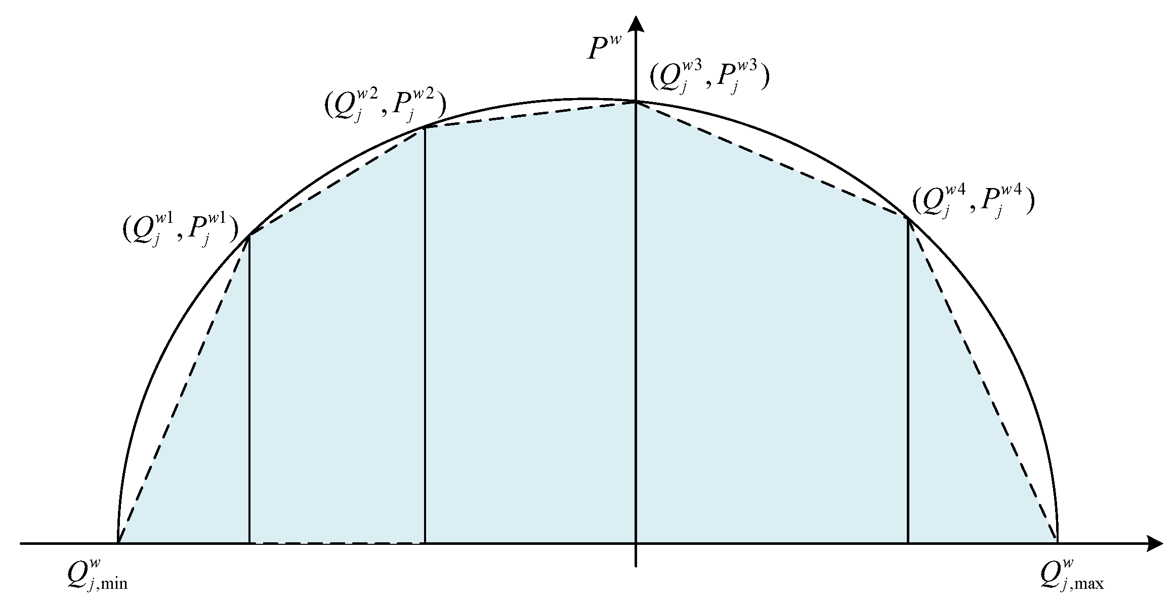
RES operation constraints:

The reactive power output of photovoltaic (PV) can be ignored, and the PV output adopts maximum power point tracking (MPPT) technology [22]:

$$P_{j,t}^v=P_{j,t}^{vm}, \forall j\in V_n$$

(23)

where $P_{j,t}^v$ and $P_{j,t}^{vm}$ are the actual active power and predicted active power of PV at timeslot t.

Similarly, the output of wind turbines (WT) can be expressed as follows:

$$P_{j,t}^w=P_{j,t}^{wm}, \forall j\in V_n$$

(24)

where $P_{j,t}^w$ and $P_{j,t}^{wm}$ are the actual active power and predicted active power of WT at timeslot t.

Taking the doubly fed induction generator (DFIG) [23], for example, the active and reactive output characteristics are shown in Figure 6.

The area surrounded by the solid line in Figure 6 is the active and reactive power operation domain of DFIG. It can be seen that it presents a strong, nonlinear coupling relationship. In order to simplify processing, the active and reactive operation domain is substituted by the shaded area, which can be expressed as the following:

$$\left\{\begin{array}{l}{P}_{j,t}^w\le \frac{P_j^{w1}}{Q_j^w-Q_{j,\min }^w}(Q_{j,t}^w-Q_{j,\min }^w)\\ P_{j,t}^w\le \frac{P_j^{w2}-P_j^{w1}}{Q_j^{w2}-Q_j^{w1}}(Q_{j,t}^w-Q_{j,t}^{w1})+P_j^{w1}\\ P_{j,t}^w\le \frac{P_j^{w3}-P_j^{w2}}{Q_j^{w3}-Q_j^{w2}}(Q_{j,t}^w-Q_{j,t}^{w2})+P_j^{w2}\\ P_{j,t}^w\le \frac{P_j^{w4}-P_j^{w3}}{Q_j^{w4}-Q_j^{w3}}(Q_{j,t}^w-Q_{j,t}^{w3})+P_j^{w3}\\ P_{j,t}^w\le \frac{P_j^{w4}}{Q_j^{w4}-Q_{\max }^w}(Q_{j,t}^w-Q_{\max }^w)+P_j^{w3}\end{array}\right.$$

(25)

where $Q_{j,t}^w$ is reactive power of WT at timeslot t. $(Q_{j,\min }^w,0)$, $(Q_{j,t}^{w1},P_{j,t}^{w1})$, $(Q_{j,t}^{w2},P_{j,t}^{w2})$, $(Q_{j,t}^{w3},P_{j,t}^{w3})$, $(Q_{j,t}^{w4},P_{j,t}^{w4})$ and $(Q_{j,\max }^w,0)$ are characteristic points of the DFIG.

4.

SVC operation constraints:

This paper assumes that reactive power compensation of the SVC is continuous:

$$Q_{C,j}^{\min }\le Q_{C,j}\le Q_{C,j}^{\max }, \forall j\in V_n$$

(26)

where $Q_{C,j}^{\max }$ and $Q_{C,j}^{\min }$ are the maximum and minimum values of the reactive power of the SVC.

2.3. The Solution Strategy of the Proposed Model

The second term in Equation (17) consists of the absolute value of the squared variables. The linearization of the objective function can reduce the computational complexity and improve the efficiency of the solution. Equation (17) can be rewritten as Equation (27) at the first step, and then $v_{b,t}^2$ and $\left|v_{b,t}\right|$ are transformed into Equation (28) by using the conventional piecewise linearization method [24]:

$$\min {\displaystyle \sum _{t=1}^{N_T}\left\{{\omega }_1{C}_{e,t}+{\omega }_2{\displaystyle \sum _{b\in V_n}(v_{b,t}^2-2\left|v_{b,t}\right|·v_{ref}+v_{ref}^2)}\right\}}$$

(27)

$$\left\{\begin{array}{l}{v}_{b,t}^2={\displaystyle \sum _{k=1}^{n_s}{\epsilon }_k}{v}_{b,t,k}^{+} , \forall b,t\\ 0\le v_{b,t,k}^{+}\le \Delta B , \forall b,t,k\\ \left|v_{b,t}\right|={\displaystyle \sum _{k=1}^{n_s}{v}_{b,t,k}^{+}} , \forall b,t\end{array}\right.$$

(28)

where $v_{b,t,k}^{+}$ and ${\epsilon }_k$ are defined as auxiliary variables. $\Delta B$ is the width of each segment in piecewise representation of the square function. $n_s$ is the number of segments. Figure 7 is the graphical illustration of the linearization method.

According to Equation (19), due to the existence of complex quadratic terms in the power flow constraint, the optimization problem is non-convex, and the distributed optimization algorithm is difficult to ensure convergence when applied to general, non-convex problems. To realize the convexity of Equation (19), $v_i^2=\frac{P_{ij}^2+Q_{ij}^2}{I_{ij}}$ can be expressed as Equations (29) and (30).

$$v_{i,t}^2{I}_{ij,t}\ge P_{ij,t}^2+Q_{ij,t}^2$$

(29)

$${‖\begin{array}{l}2P_{ij,t}\\ 2Q_{ij,t}\\ I_{ij,t}-V_{i,t}^{}\end{array}‖}_2\le I_{ij,t}+V_{i,t}^{}$$

(30)

Based on the piecewise linearization of the objective function and the convexity of the power flow constraint, a decentralized algorithm, which is developed based on the ADMM, is introduced to the model solution in order to reduce the computational burden.

In order to realize decentralized optimization, the power of EVA is used as the coupling variable to establish the coupling constraint. Therefore, at the node i, which contains EVA, a set of virtual variables representing the injected power of EVA nodes are added, relative to the injected power of the ADN side. The scheme in Figure 8 is adopted to realize the decoupling between the ADN side and EVA side.

Based on the decomposition scheme of ADN and EVA sides, the optimization task can be expressed as follows:

$$\mathrm{F}=\min {\displaystyle \sum _{t=1}^{N_T}\left\{{\omega }_1{C}_{e,t}+{\omega }_2{\displaystyle \sum _{b\in V_n}({\displaystyle \sum _{k=1}^{n_s}{\epsilon }_k}{v}_{b,t,k}^{+}-2v_{ref}{\displaystyle \sum _{k=1}^{n_s}{v}_{b,t,k}^{+}}+v_{ref}^2)}\right\}}$$

(31)

$$\mathrm{subject} \mathrm{to} \left\{\begin{array}{l}\mathrm{AND} \mathrm{side}: (18)-(26),(28),(30)\\ \mathrm{EVA} \mathrm{side}: (1)-(16)\\ \mathrm{Coupling} \mathrm{point}: P_{i,t}^{\prime }=P_{i,t},Q_{i,t}^{\prime }=Q_{i,t}.\forall i\in A_a,t\in N_T\end{array}\right.$$

(32)

The objective function (31) is quadratic constrained linear programming and the ADMM is used for the implementation of the distributed solution in this paper. The coordination of the injected power ($P_i$,$Q_i$) on the ADN side and the injected power ($P_i^{\prime }$,$Q_i^{\prime }$) on the EVA side are achieved by adding the Lagrange penalty function into the objective function. The suboptimal models of EVA and ADN can be expressed as Equations (33) and (34).

$$\left\{\begin{array}{c}min\sum _{t=1}^{N_T}\left\{F_1\right.+\sum _{i\in A_a}[{\kappa }_{i,t}·(P_{i,t}-\widehat{P_{i,t}^{{}^{\prime }}})+{\delta }_{i,t}(Q_{i,t}-\widehat{Q_{i,t}^{{}^{\prime }}})]+\frac{\rho }{2}\sum _{t=1}^{N_T}\sum _{i\in A_a}[{\kappa }_{i,t}(P_{i,t}-\widehat{P_{i,t}^{{}^{\prime }}})+{\delta }_{i,t}(Q_{i,t}-\widehat{Q_{i,t}^{{}^{\prime }}}){]}^2\}\hfill \\ F_1={\omega }_1·[{\gamma }_t\sum _{b\in V_n}(P_{b,t}^L-P_{b,t}^G)+C_{g,t}]+{\omega }_2\sum _{b\in V_n}(\sum _{k=1}^{n_s}{\epsilon }_k{v}_{b,t,k}^{+}-2v_{ref}\sum _{k=1}^{n_s}{v}_{b,t,k}^{+}+v_{ref}^2)\hfill \end{array}\right.$$

(33)

s.t. Equations (18)–(26), (28), (30)

$$\left\{\begin{array}{l}\min {\displaystyle \sum _{t=1}^{N_T}\left\{F_2\right.}+{\displaystyle \sum _{i\in A_a}[{\kappa }_{i,t}}·(\widehat{P_{i,t}}-P_{i,t}^{\prime })+{\delta }_{i,t}(\widehat{Q_{i,t}}-Q_{i,t}^{\prime })]+\frac{\rho }{2}{\displaystyle \sum _{t=1}^{N_T}{\displaystyle \sum _{i\in A_a}[{\kappa }_{i,t}(}}\widehat{P_{i,t}}-P_{i,t}^{\prime })+{\delta }_{i,t}(\widehat{Q_{i,t}}-Q_{i,t}^{\prime }){]}^2\}\\ F_2={\gamma }_t{P}_{es}(t)+{\omega }_1{C}_{A,t}\end{array}\right.$$

(34)

s.t. Equations (1)–(16)

where $\widehat{P_{i,t}}$, $\widehat{Q_{i,t}}$, $\widehat{P_{i,t}^{\prime }}$ and $\widehat{Q_{i,t}^{\prime }}$ are the optimal solution; ${\kappa }_{i,t}$ and ${\delta }_{i,t}$ are Lagrangian multipliers; and $\rho$ is the penalty factor of ADMM. Suboptimal models of ADN and EVA are solved independently, and the boundary variable information is exchanged until the convergence conditions are met:

$${\displaystyle \sum _{t=1}^{N_T}{\displaystyle \sum _{i\in A_a}{\left|\widehat{P_{i,t}}(r)-\widehat{P_{i,t}^{\prime }}(r)\right|}^2}}+{\left|\widehat{Q_{i,t}}(r)-\widehat{Q_{i,t}^{\prime }}(r)\right|}^2\le \epsilon$$

(35)

where $r$ and $\epsilon$ are the number of iterations and threshold of convergence criteria, separately.

The specific steps of the distributed optimization solution based on ADMM are as follows:

Step 1: Initialize variables $\widehat{P_{i,t}}(0)$, $\widehat{P_{i,t}^{\prime }}(0)$, $\widehat{Q_{i,t}}(0)$, $\widehat{Q_{i,t}^{\prime }}(0)$, ${\kappa }_{i,t}$(0) and ${\delta }_{i,t}$(0), and set r = 1.

Step 2: EVA optimizes Equation (34) and transmits the optimization results $\widehat{P_{i,t}^{\prime }}$ and $\widehat{Q_{i,t}}$ to ADN.

Step 3: ADN optimizes the model of Equation (33) after it receives the optimization results of EVA and passes the optimization results $\widehat{P_{i,t}}$ and $\widehat{Q_{i,t}}$ to EVA.

Step 4: The convergence test is carried out according to Equation (35). If satisfied, the optimization is completed, and the optimized results are outputted. Otherwise, ${\kappa }_{b,t}$ and ${\delta }_{b,t}$ are updated according to Equation (36). Set the number of iterations r = r + 1. Return to Step 2.

$$\left\{\begin{array}{l}{\kappa }_{b,t}(r+1)={\kappa }_{b,t}(r)+\rho [\widehat{P_{i,t}}(r)-\widehat{P_{i,t}^{\prime }}(r)]\\ {\delta }_{b,t}(r+1)={\delta }_{b,t}(r)+\rho [\widehat{Q_{i,t}}(r)-\widehat{Q_{i,t}^{\prime }}(r)]\end{array}\right.$$

(36)

3. Results and Discussion

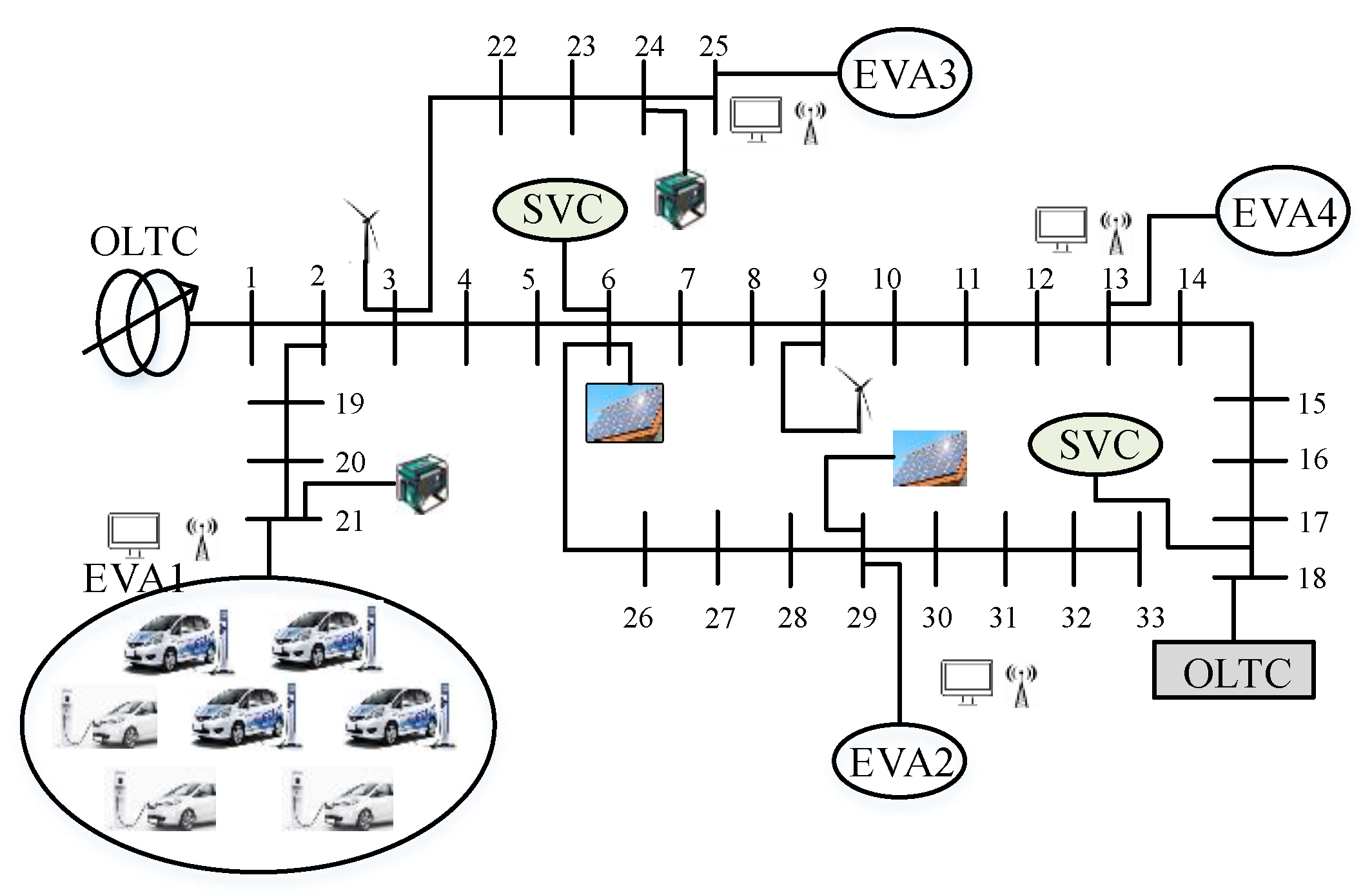
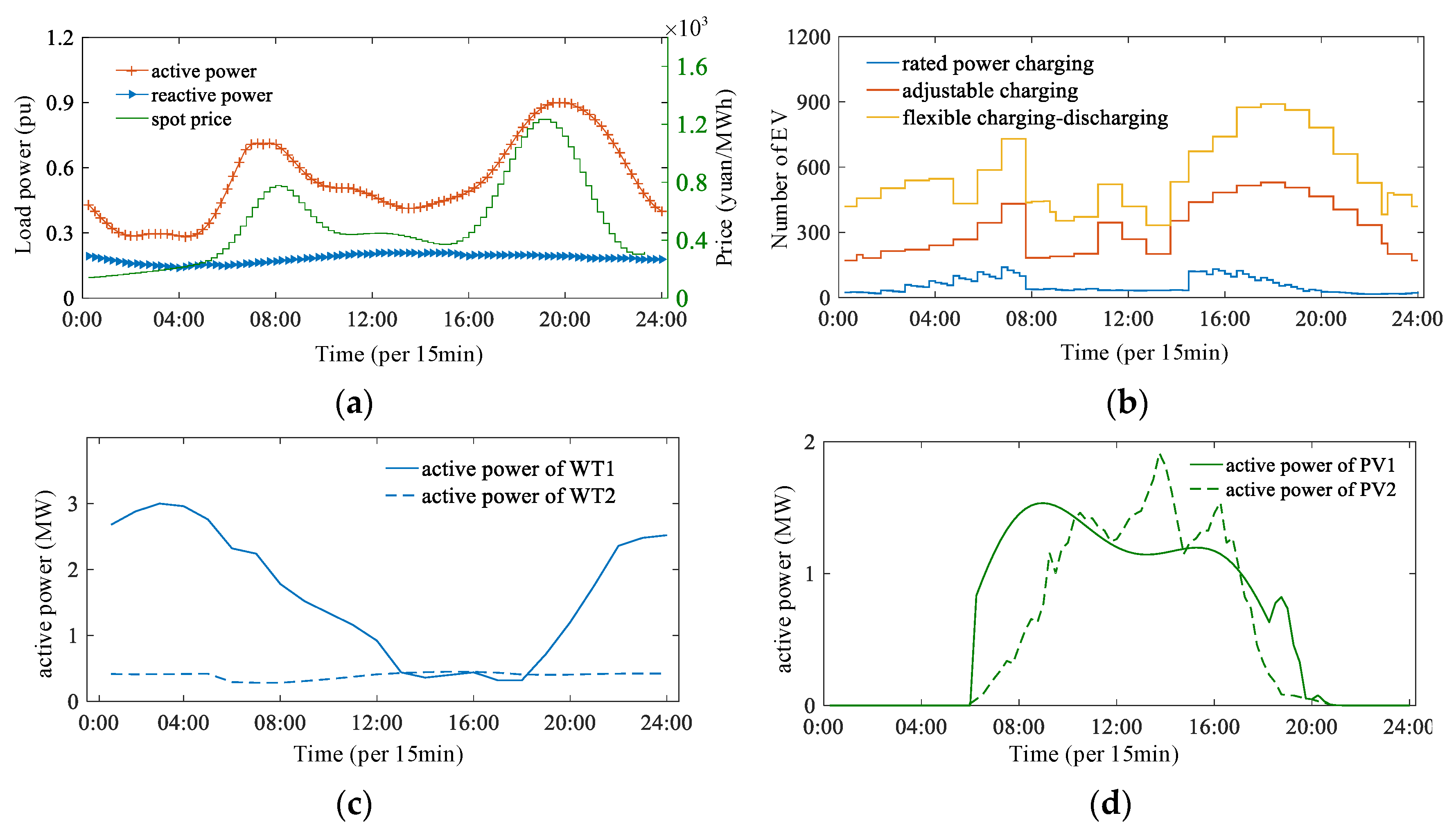
3.1. System Data

In this paper, the numerical test is based on the radial cable 33-bus ADN with a normal voltage of 12.66 kV. The line parameters of the ADN can be found in reference [25]. The optimization horizon is 24 h of a day, which is divided into N_T = 96 timeslots. The value of $\epsilon$ is set as 10⁻⁴. Figure 9 shows the topology of the ADN. Without loss of generality, it is assumed that all conventional loads are residential loads with known load curves as illustrated in Figure 10a. The green curve in Figure 10a shows the spot price of active power, which is associated with a typical day [26]. The value of ${\beta }_t$ is equal to half of the spot price in this paper. In the test case, there are four EVAs that are connected to buses 13, 21, 25, 29, and the maximum acceptable numbers of EVs are 500, 500, 750, 900, respectively. To simplify the calculation, it is assumed that all EVs are of the same type, and the ratio of the rated power charging EVs, non-discharging EVs and flexible charging–discharging EVs is 2:3:5.

Table 1. The parameters of FGs.

Parameters	FG1	FG2
Pmin/MW	1	1.5
Pmax/MW	3	5
Qmin/MVar	−0.5	−0.5
Qmax/MVar	1.5	1.5
Pdmax/MW·Δt	2	3.5
Pumax/MW·Δt	2	3.5
γ/MW	600	800
a/yuan	180	150
b/yuan·MW	480	450
c/yuan·MW2	0.021	0.820
s/yuan	60	90

and

Table 2. The parameters of plugged-in EVs.

Parameters	Value
Pc/kW·h	10
Pd/kW·h	10
ηc	0.95
ηd	0.95
E/kW·h	40
Sex	0.95
Sthr	0.5

show the FG parameters and EV parameters, respectively. Meanwhile, the probability distribution of the EVs’ arrival–departure time and daily mileage were obtained from the literature [27]. Then, the Monte Carlo method is used to calculate the number of EVs plugged into the ADN in a day as shown in Figure 10b. The output of WT and PV are shown in Figure 10c,d.

The test case is solved by programming in the environment of MATLAB 2016a. Meanwhile, the CPLEX 12.6 solver is employed.

As summarized in

Table 3. The characteristics of multiple cases.

Cases	EV Control Capability			Characteristics
	Users’ Preference	Active Power	Reactive Power
Case I	✕	✕	✕	No reactive power. All EVs are charged with rated active power.
Case II	✕	✓	✓	Regardless of preference of EV users. Operation with both active power and reactive power.
Case III	✓	✓	✕	Considering preference of EV users. Operation with only active power.
Case IV	✓	✓	✓	Considering preference of EV users. Operation with both active power and reactive power.

, four different cases are analyzed to investigate employing EVs’ conjugate active and reactive power control capabilities in an ADN operation. The preference of EV users are ignored in case I and case II. In case I, all EVs plugged-in are charged with rated active power, and the reactive power is zero. In case II, all EVs are supposed to be flexible charging–discharging for which both the active power and reactive power are adjustable. The preference of EV users is considered in case III and case IV. In case III, the reactive power of EVs is zero and the active power is adjustable, except for EVs charged with rated power. In case IV, for an adjustable charging EV, the operation domain of the active and reactive power is shown in Figure 5a; for a flexible charging–discharging EV, the operation domain of the active and reactive power is illustrated in Figure 5b.

3.2. Study Results and Discussions

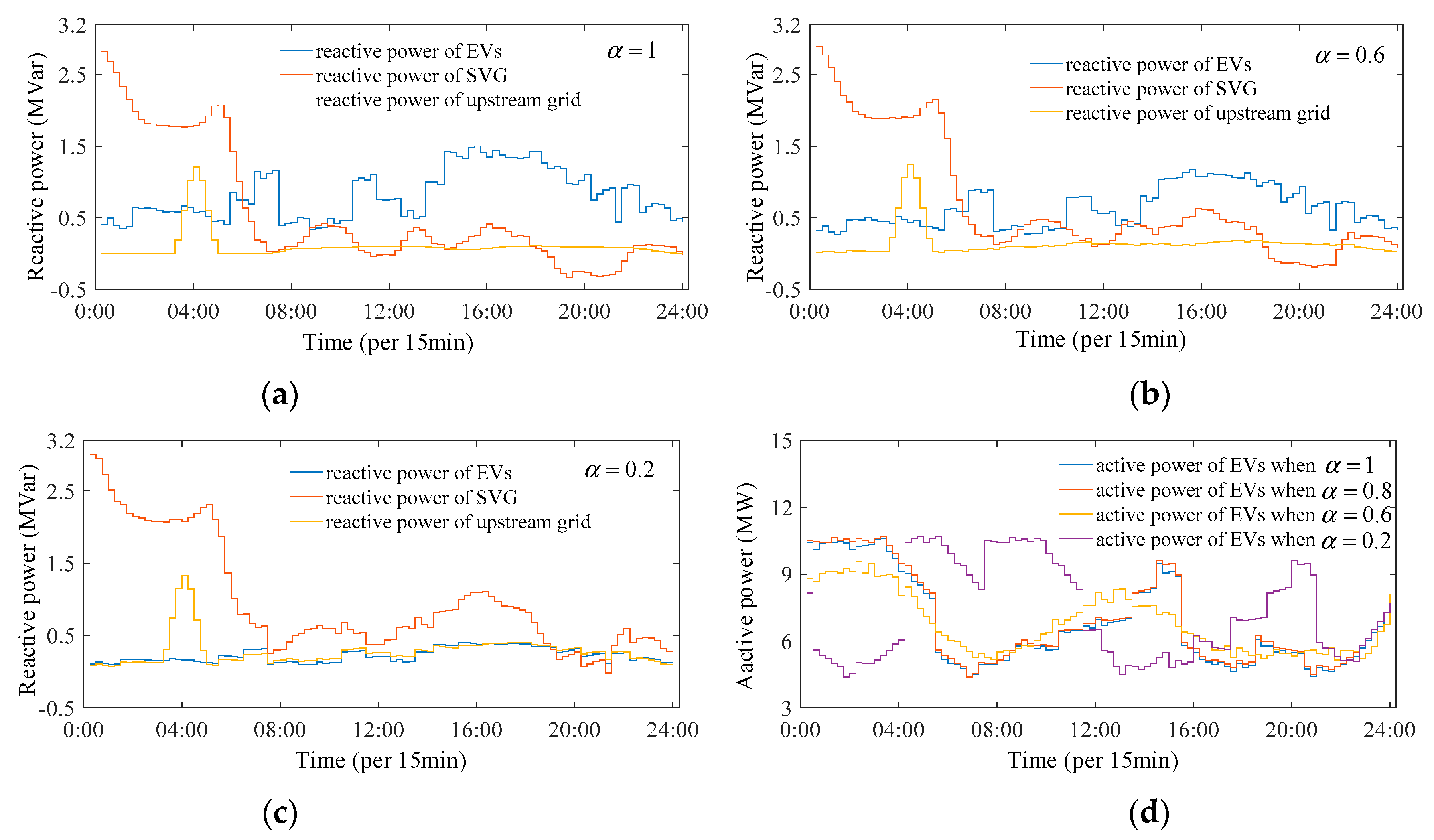
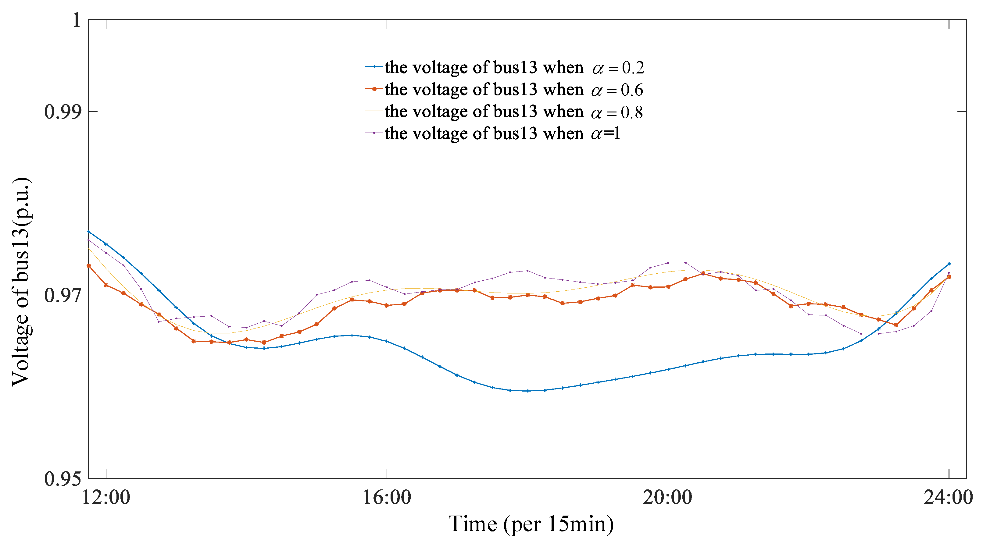
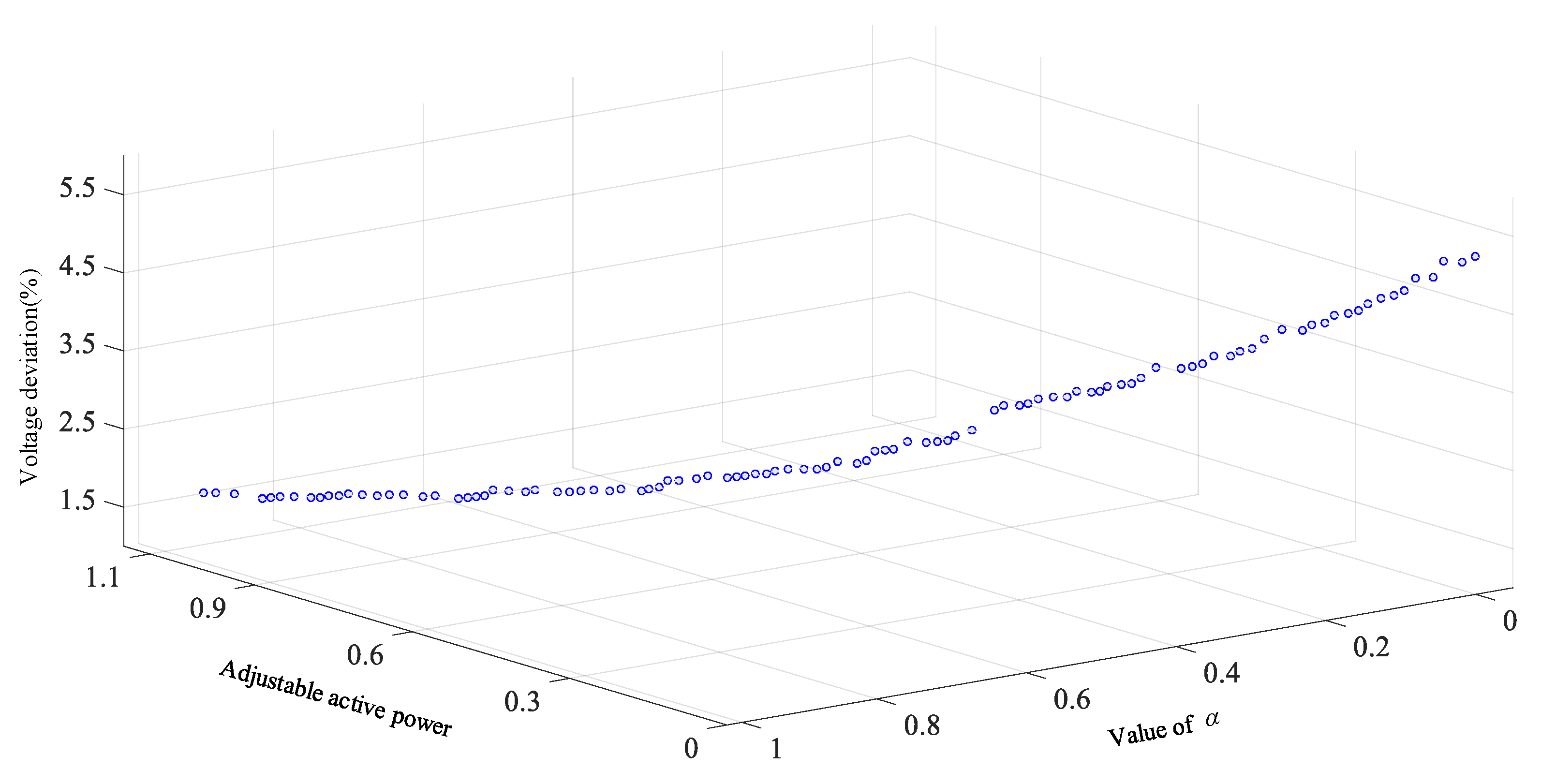
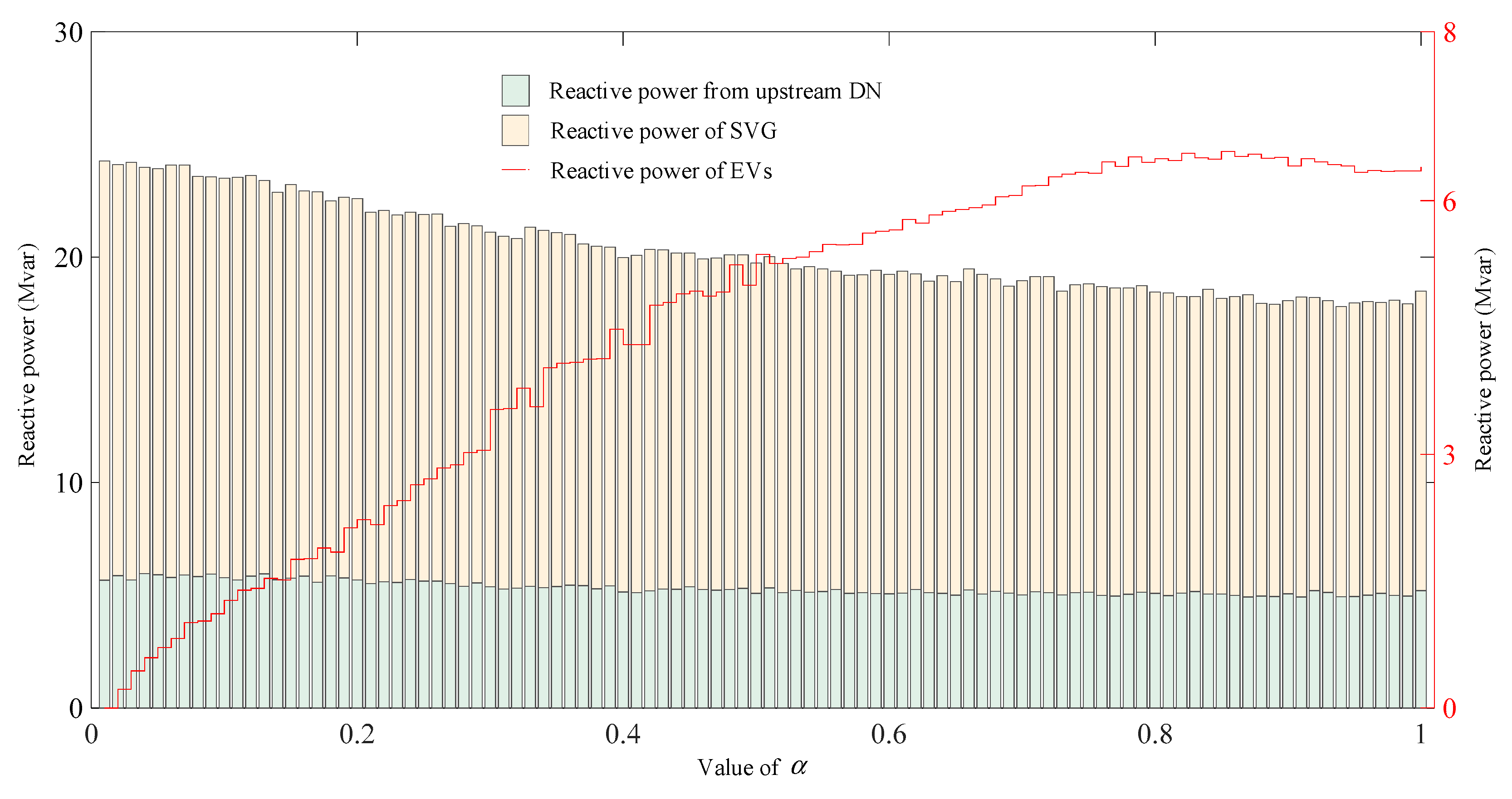
3.2.1. Coefficients Selection of Objective Function

It can be seen, according to Equation (31), that the two terms of the objective function are the total cost of energy and the summation of the voltage deviation, respectively.

Table 4. Influence of different values for coefficients of ${\omega }_1$, ${\omega }_2$.

Items	Values of ${\mathit{\omega }}_1$ and ${\mathit{\omega }}_2$
Weight coefficient	${\omega }_1$ = 1, ${\omega }_2$ = 0	${\omega }_1$ = 0, ${\omega }_2$ = 1	${\omega }_1$ = 5.58 × 10−5${\omega }_2$
Energy cost (CNY)	5.75 × 104	6.08 × 104	5.93 × 104
Voltage profile (p.u.)	1.107	0.923	0.975

shows the results of the two terms of the objective function under different values for ${\omega }_1$ and ${\omega }_2$. According to Table 4, in the case of ${\omega }_1$ = 1, ${\omega }_2$ = 0 (${\omega }_1$ = 0, ${\omega }_2$ = 1), the energy cost (voltage profile) is considered the only objective function. In the third case, the value of ${\omega }_1$ is set to be equal to 5.58 × 10⁻⁵ ${\omega }_2$. The meaning of this value selection is expressed as follows:

According to the results given in Table 4, it can be found that the maximum and minimum values of the total energy cost are CNY 6.08 × 10⁴ and CNY 5.75 × 10⁴, respectively. Meanwhile, the maximum and minimum values of voltage are 1.107 p.u. and 0.923 p.u., respectively. Therefore, it can be concluded that the value spans of two parts of the objective function (i.e., total energy cost and voltage profile) are 3300 and 0.184, respectively. To make the two parts of the objective function have the same standard, the first part of the objective function (total energy cost) is divided by CNY 3300 and the second part of the objective function (voltage profile) is divided by 0.184 p.u. In other words, this means that we evaluate ${\omega }_1$ and ${\omega }_2$ in such a way that ${\omega }_1$ = 5.58 × 10⁻⁵ ${\omega }_2$ (${\omega }_1$ = 0.184/3300 ${\omega }_2$). By setting two weight coefficients in this way, the two parts of the objective function are equally weighted.

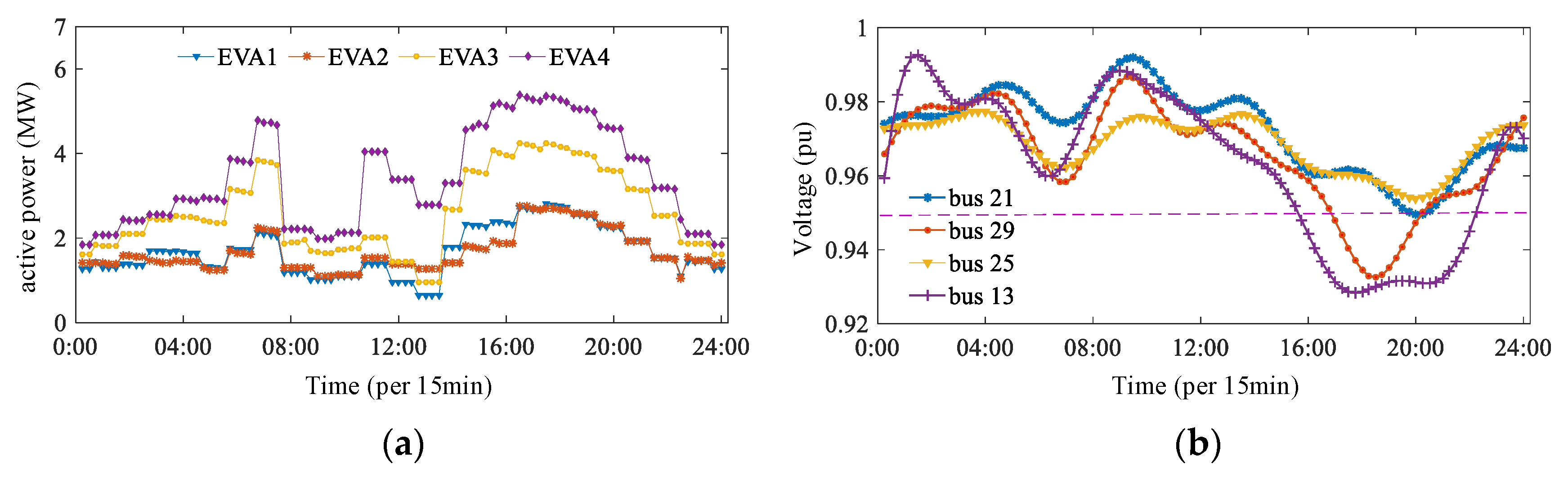
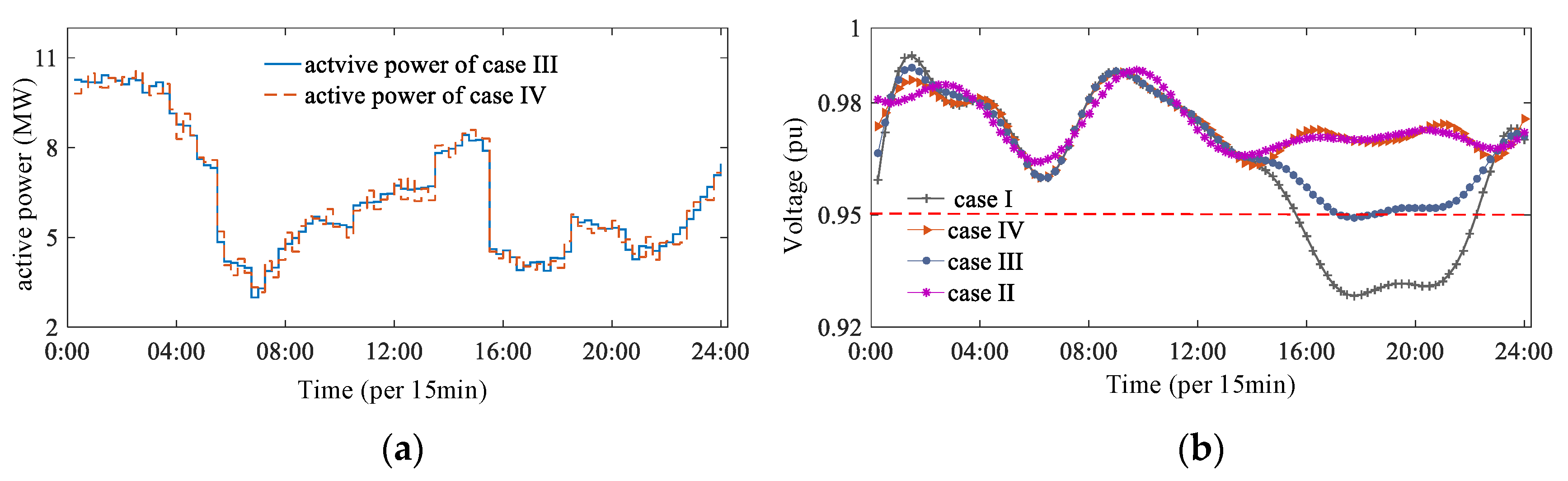
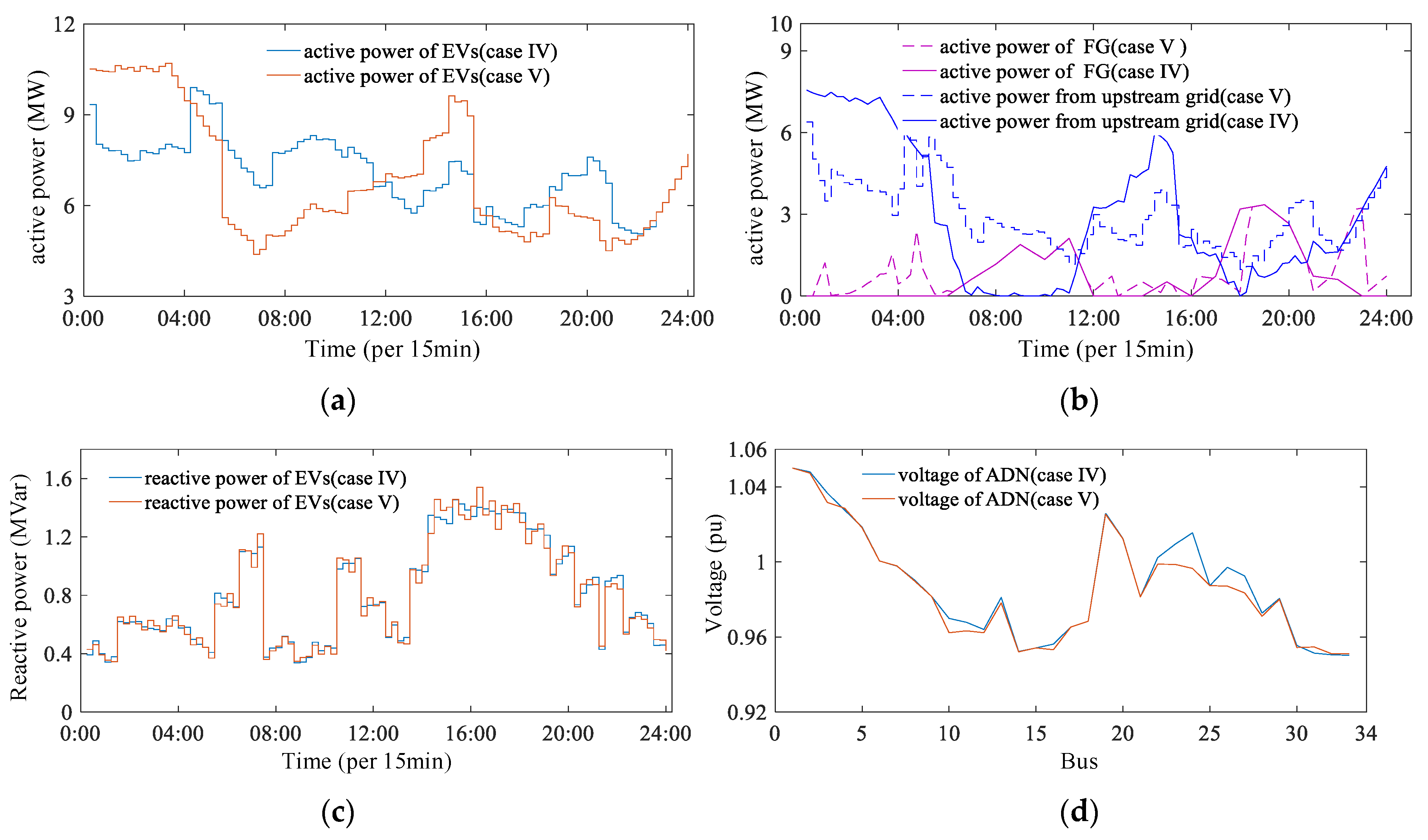
3.2.2. Analysis of Different Test Cases

In case I, the reactive power capacity of EVs is not considered, and the active power of EV is not controllable. Once the EV is plugged into ADN, it is charged to the desired SOC with the rated active power. By comparing the active conventional load curves in Figure 10a and Figure 11a, it can be seen that the load peak and valley of EVs and the conventional load are simultaneous, and the superposition of the two loads obviously further aggravates the load fluctuation of the ADN. Figure 11b shows that, due to the superposition of the peak load, the voltage at nodes 13 and 29 in peak intervals deviates from the normal voltage range, which poses a great threat to the operation safety of the ADN. Therefore, it is very important to achieve optimal control of plugged-in EVs.

Comparing case II and case IV, as shown in Figure 12a, the adjustable range of active power in case II is larger than case IV (yellow area for case IV, green and yellow area for case II). The reason for this is that the preference of EV users is taken into account in case IV; some EVs need to be charged at the rated power, so the active power is not adjustable. In contrast, the active power of all EVs in case II is adjustable. The solid red and green lines in Figure 12a represent the EVs’ load curves of case II and case IV, respectively. A larger number of EVs are plugged into ADN from 18:00 to 24:00; some EVs must be charged at the rated power in case IV, which results in a greater active power than that for case II. In case IV, once the EV charging at the rated power reaches the desired SOC, the charging process stops and the total active power may be lower than that in case II (e.g., 00:00–06:00).

Figure 12b shows the summation of EVs’ reactive power in cases II and IV. It can be seen that the reactive power curves of the two schemes are similar. Since both cases have enough EVs whose charging power can be regulated, the required reactive power of the ADN can be provided sufficiently in both cases based on the intelligent bi-directional charger.

As the number of EVs charged by rated power is small, it can be seen from Figure 12c that whether the preference of users is considered has little influence on the voltage amplitude of the ADN. However, by comparing Figure 11b and Figure 12c, it can be concluded that the voltage profiles of buses 13 and 29 during peak load hours could be improved noticeably, while both the active and reactive power of EVs are controllable. Figure 12d illustrates the voltage magnitude of the ADN in case II; the bus voltage magnitude is in the acceptable range (0.95–1.05 p.u.).

In order to evaluate the advantages of employing the EVs’ reactive power control capability more directly and accurately, case III and case IV are compared, and the results are shown in Figure 13, Figure 14 and Figure 15. The only difference between the two cases is that the reactive power control capability of EVs is considered in case IV. It can be seen from Figure 13a that, over 96 intervals throughout the day, the difference of active power between the two cases is not significant. Figure 13b shows the significant improvement of the voltage profile (especially in the 14:00–22:00 intervals) of bus 13 by employing the reactive power control (case IV) of EVs. Meanwhile, combined with the analysis in Figure 14, the reactive power compensation provided by SVG in case IV is significantly less than that in case III. The reactive power obtained from the upstream DN is also less than that of case III. It can be concluded that employing the reactive power control capability of EVs can not only improve the voltage profile, but also reduce the capacity of SVG configuration in the ADN and save the investment cost of the ADN. Figure 15 shows that the implementation of the chargers’ reactive power capability prevents severe voltage drop of the buses.

Combined with the analysis in Figure 10a, Figure 13a and Figure 16, on the one hand, the active power control ability of EVs plays the effect of peak clipping and valley filling to some extent. On the other hand, due to the energy cost term in the objective function, EVs absorb more power during the off-peak intervals, which is beneficial for EV users to reduce the charging cost. From the perspective of ADN operation, the ADN absorbs more power from the upstream DN in the period when the market electricity price is lower; in the period when the electricity price is higher, the ADN fully mobilizes the active power of FGs, thus reducing the operation cost of the ADN.

3.2.3. Charging Process under Demand Preference

To be more intuitive, $l_{m,k}$($m=1,2,3$,$k=1,2,3,4$) is an EV randomly selected from $D_{m,k}$ in case IV. The SOC curve of $l_{m,k}$ is shown in Figure 17.

The SOC of the three categories of EVs in EVA₁–EVA₄ is above 0.95 when they are off-grid, which fully guarantees the users’ energy demands. Whenever the $l_{1,k}$ is plugged into the ADN, it is charged at $P_{c,l}^r$ until the desired SOC is reached; during the plugged-in intervals, the actual charging power of $l_{2,k}$ is less than $P_{c,l}^r$, and the value of SOC increases slowly but there is no discharge process over its plugged-in intervals. Part of the plugged-in intervals of $l_{3,k}$ are in the discharging state, but the SOC during the discharging process is higher than the threshold value of 0.5. It should be noted that the EV in $D_{2,k}$ or $D_{3,k}$ set is also constrained by both the plugged-in duration and energy demand. When the plugged-in duration is shorter and the energy demand is larger, although its active power is adjustable, it still maintains a high charging power in order to meet the energy demand, such as $l_{2,2}$, $l_{3,4}$. Obviously, the optimization model established in this paper sufficiently guarantees the demand preference of EV users.

3.3. Superiority Analysis of the Proposed Model

The model established in this paper quantifies the reactive power capacity of EV more accurately, and fully guarantees the preference of the users. However, none of the existing literature takes both of these two points into account. Therefore, to further verify the advantages of the distributed optimization strategy proposed in this paper, the proposed strategy is compared with the strategy of the stochastic, multi-objective based on normalized normal constraint (NNC) method proposed in reference [14]. It should be pointed out that the framework of the test case in reference [14] is significantly different from that in this paper. Therefore, we only use the theoretical method in reference [14] (defined as case V) to solve the test case (case IV) in this paper, and the objective function is also transformed into the multi-objective form. The comparison of the optimization results between case IV and case V are shown in Figure 18 and

Table 5. The objective function value and the solving time in case IV and case V.

Case	Energy Cost (CNY)	Voltage Deviation (%)	The Solving Time (s)
Case IV	5.93 × 104	1.17%	202.3
Case V	7.02 × 104	1.26%	621.7

.

According to Figure 18 and Table 5, it can be seen that the difference in the active power optimization results is great, and the difference in the reactive power optimization is small. The total energy costs of case IV and case V are significantly different, but the difference in the average voltage deviation is not significant. Compared with that of case V, the total energy cost of case IV is reduced by CNY 1.09 × 10⁴. More significantly, the solving time of the two cases is greatly different. The distributed optimization strategy proposed in this paper only needs one third of the time compared to reference [14]. The solution efficiency is greatly improved in this paper.

3.4. Analysis in EVs Penetration Point of View

In this section, case IV is also taken as an example to analyze the influence of different EVs’ distributions on the proposed model. The different distributions of EVs include two aspects: For the first one, the proportions of the three categories of EVs are different. The other is that the number of EVs is different. The second aspect is reflected in the test cases (the number of EVs managed by four EVAs is different). For the first aspect, the test scheme is designed as follows:

Firstly, define $\alpha$ to be the ratio of EVs in the $D_{2,k}$ and $D_{3,k}$ set. So, $\alpha =0.8$ in Section 3.2. Figure 19 shows the reactive power of the EVs, SVG, upstream grid and active power of EVs when the value of $\alpha$ is equal to 0.2, 0.6 and 1, respectively.

According to Figure 19a–c, the reactive power from the upstream grid and the reactive power of EVs and SVG have a slight difference in the case of $\alpha =1$ or $\alpha =0.6$. This is because the ratio of EVs in $D_{2,k}$ and $D_{3,k}$ sets is relatively high, which provide sufficient reactive power. When $\alpha =0.2$, most EVs are charged at the rated power, and the reactive power provided by the smart charger is significantly reduced, while the reactive power compensated by SVC is significantly increased, which means that the SVG configuration capacity in the ADN needs to be increased. Comparing Figure 10d with Figure 19d, it can be seen that the smaller the value of $\alpha$, the more obvious the peak–valley simultaneity for both the EVs’ load and conventional load and the worse the effect of load shifting.

Figure 20 shows the voltage profile of bus 13 under different values of $\alpha$. As the value of $\alpha$ increases, the voltage profile of bus is improved. However, when $\alpha$ = 0.8 or $\alpha$ = 1, there is little improvement in the voltage profile of bus 13, compared to $\alpha =0.6$.

In order to intuitively show the relationship between the $\alpha$ value and the adjustable active power and voltage deviation, ${\gamma }_p$ is defined as the mean value of the adjustable active power of EVs over 96 intervals, and ${\gamma }_v$ is defined as the mean value of the voltage deviation from the standard voltage over 96 intervals.

Then, 100 different values of $\alpha$ between 0 and 1 are taken (the equal step size of 0.01 is taken in this paper). Other conditions are consistent with case IV. The relationship between ${\gamma }_p$, ${\gamma }_v$ and $\alpha$ is shown in Figure 21.

The scattered points in Figure 21 can be approximated as a spatial curve. When $\alpha$ = 0, every EV is charged at the rated charging power, so the active power is not adjustable; then, ${\gamma }_p$ = 0 and ${\gamma }_v$ reaches the maximum value of 5.5%. With the increase in $\alpha$, ${\gamma }_p$ increases and ${\gamma }_v$ decreases but the decreasing trend of ${\gamma }_v$ tends to be moderate. This is because when the EVs in $D_{2,k}$ and $D_{3,k}$ sets reach a certain amount, sufficient reactive power capacity is provided, so the value of ${\gamma }_v$ does not have a significant change.

The results in Figure 22 are the sum of the reactive powers over 96 intervals. With the increasing proportion of EVs in $D_{2,k}$ and $D_{3,k}$ sets, the reactive power injected by SVG gradually decreases, while the reactive power injected by EVs gradually increases, and both trends tend to smoothen gradually. The reactive power absorbed by the ADN from the upstream DN is relatively stable.

4. Conclusions and Future Works

Based on an intelligent charger capable of four-quadrant operation and the scenario of large-scale, EV penetration, in this paper, an energy optimization model for the ADN, by employing cooperative active and reactive power management of EVs, is proposed. Some numerical case studies were investigated to demonstrate the superiority of the proposed model. The main achievements are summarized as follows:

(1)

The total energy cost is reduced and the voltage profile of ADN is improved by employing the model proposed in this paper. The energy cost is reduced by about 15.5 percent, and the voltage profile is improved by about 0.09 percent.

(2)

The demand preference of EV users is taken into account in the proposed model. The plugged-in EVs are divided into three categories: rated power charging EVs, non-discharging EVs, and flexible charging–discharging EVs. Users can choose different charging modes, which are more in line with the actual scenario. The study results show that the proposed model can fully guarantee the users’ demand preference.

(3)

A distributed solution strategy based on ADMM is designed for the proposed model. The experimental results show that the distributed strategy proposed in this paper can save about two thirds of the solving time.

The following aspects are worthy of further study in the future.

(1)

Uncertainty: There are multiple uncertainties, such as the arrival and departure time of EVs, active power of WT and PV, system failure, and so on. The question of how to consider these uncertainties in the established model needs further research.

(2)

Interactivity: In practice, users can interact with the EVA by making an appointment to charge, switching charging modes, adjusting the charging power or discharging power, and so on. The question of how to improve the model to meet the timely interaction between the EV and EVA is another direction to be further studied.

References

1. Kumar, M.D.; Jabbari, G.M.; Ali, A.; Li, L.; Jiangfeng, Z. A review on resilience studies in active distribution systems. Renew. Sustain. Energy Rev. 2021, 135, 110201. [Google Scholar]
2. Flammini, M.G.; Prettico, G.; Julea, A.; Fulli, G.; Mazza, A.; Chicco, G. Statistical characterisation of the real transaction data gathered from electric vehicle charging stations. Electr. Power Syst. Res. 2018, 166, 136–150. [Google Scholar] [CrossRef]
3. Singh, J.; Tiwari, R. Electric vehicles reactive power management and reconfiguration of distribution system to minimise losses. IET Gener. Transm. Distrib. 2020, 14, 6285–6293. [Google Scholar] [CrossRef]
4. Wei, C.; Xu, J.; Liao, S.; Sun, Y. Aggregation and Scheduling Models for Electric Vehicles in Distribution Networks Considering Power Fluctuations and Load Rebound. IEEE Trans. Sustain. Energy 2020, 11, 2755–2764. [Google Scholar] [CrossRef]
5. Hongesombut, K.; Punyakunlaset, S.; Romphochai, S. Under Frequency Protection Enhancement of an Islanded Active Distribution Network Using a Virtual Inertia-Controlled-Battery Energy Storage System. Sustainability 2021, 13, 484. [Google Scholar] [CrossRef]
6. Abessi, A.; Shirazi, E.; Jadid, S.; Shafie-khah, M. Sustainable and Resilient Smart House Using the Internal Combustion Engine of Plug-in Hybrid Electric Vehicles. Sustainability 2020, 12, 6046. [Google Scholar] [CrossRef]
7. Wu, J.; Hu, J.; Ai, X.; Zhang, Z.; Hu, H. Multi-time scale energy management of electric vehicle model-based prosumers by using virtual battery model. Appl. Energy 2019, 251, 113312. [Google Scholar] [CrossRef]
8. Shi, R.; Li, S.; Zhang, P.; Lee, K. Integration of renewable energy sources and electric vehicles in V2G network with adjustable robust optimization. Renew. Energy 2020, 153, 1067–1080. [Google Scholar] [CrossRef]
9. Meesenburg, W.; Thingvad, A.; Elmegaard, B.; Marinelli, M. Combined provision of primary frequency regulation from Vehicle-to-Grid (V2G) capable electric vehicles and community-scale heat pump. Sustain. Energy Grids Netw. 2020, 23, 100382. [Google Scholar] [CrossRef]
10. Dong, C.; Chu, R.; Morstyn, T.; Mcculloch, M.; Jia, H. Online Rolling Evolutionary Decoder-Dispatch Framework for the Secondary Frequency Regulation of Time-Varying Electrical-Grid-Electric-Vehicle System. IEEE Trans. Smart Grid 2021, 12, 871–884. [Google Scholar] [CrossRef]
11. Pirouzi, S.; Aghaei, J.; Niknam, T.; Khooban, M.H.; Dragicevic, T.; Farahmand, H.; Korpas, M.; Blaabjerg, F. Power Conditioning of Distribution Networks via Single-Phase Electric Vehicles Equipped. IEEE Syst. J. 2019, 13, 3433–3442. [Google Scholar] [CrossRef] [Green Version]
12. Pirouzi, S.; Latify, M.A.; Yousefi, G.R. Conjugate active and reactive power management in a smart distribution network through electric vehicles: A mixed integer-linear programming model. Sustain. Energy Grids Netw. 2020, 22, 100344. [Google Scholar] [CrossRef]
13. Fu, Y.; Meng, X.; Su, X.; Jabalameli, N.; Dong, Z. Coordinated optimisation of PEV charging with the support of reactive discharging and phase switching in unbalanced active distribution networks. IET Gener. Transm. Distrib. 2020, 14, 4703–4710. [Google Scholar] [CrossRef]
14. Saffari, M.; Kia, M.; Vahidinasab, V.; Mehran, K. Integrated active/reactive power scheduling of interdependent microgrid and EV fleets based on stochastic multiobjective normalised normal constraint. IET Gener. Transm. Distrib. 2020, 14, 2055–2064. [Google Scholar] [CrossRef]
15. Sousa, T.; Hashemi, S.; Andersen, P.B. Raising the potential of a local market for the reactive power provision by electric vehicles in distribution grids. Gener. Transm. Distrib. IET 2019, 13, 2446–2454. [Google Scholar] [CrossRef] [Green Version]
16. Kikusato, H.; Mori, K.; Yoshizawa, S.; Fujimoto, Y.; Asano, H.; Hayashi, Y.; Kawashima, A.; Inagaki, S.; Suzuki, T. Electric Vehicle Charge-Discharge Management for Utilization of Photovoltaic by Coordination between Home and Grid Energy Management Systems. IEEE Trans. Smart Grid 2019, 10, 3186–3197. [Google Scholar] [CrossRef]
17. Wang, P.; Zou, S.; Ma, Z. A Partial Augmented Lagrangian Method for Decentralized Electric Vehicle Charging in Capacity-Constrained Distribution Networks. IEEE Access 2019, 7, 118229–118238. [Google Scholar] [CrossRef]
18. Clairand, J.-M. Participation of Electric Vehicle Aggregators in Ancillary Services Considering Users’ Preferences. Sustainability 2020, 12, 8. [Google Scholar] [CrossRef] [Green Version]
19. Engr, B.; Lek, A.; Erenolu, A.K.; Erdin, O.; Catalo, J. User-comfort oriented optimal bidding strategy of an electric vehicle aggregator in day-ahead and reserve markets. Int. J. Electr. Power Energy Syst. 2020, 122, 106194. [Google Scholar]
20. He, T.; Lu, D.C.; Wu, M.; Yang, Q.; Li, T.; Liu, Q. Four-Quadrant Operations of Bidirectional Chargers for Electric Vehicles in Smart Car Parks: G2V, V2G, and V4G. Energies 2020, 14, 181. [Google Scholar] [CrossRef]
21. Monsef, H.; Siano, P. Design of a risk-averse decision making tool for smart distribution network operators under severe uncertainties: An IGDT-inspired augment ε-constraint based multi-objective approach. Energy 2016, 116, 214–235. [Google Scholar]
22. Kanagaraj, N. Photovoltaic and Thermoelectric Generator Combined Hybrid Energy System with an Enhanced Maximum Power Point Tracking Technique for Higher Energy Conversion Efficiency. Sustainability 2021, 13, 3144. [Google Scholar]
23. Qing, M.; Tang, F.; Liu, F.; Liu, D.; Du, N.; Hu, B. An Analytical Method for Estimating the Maximum Penetration of DFIG Considering Frequency Stability. Sustainability 2020, 12, 9850. [Google Scholar] [CrossRef]
24. Jovanović, J.; Denić, D. A Cost-effective Method for Resolution Increase of the Twostage Piecewise Linear ADC Used for Sensor Linearization. Meas. Sci. Rev. 2016, 16, 28–34. [Google Scholar] [CrossRef] [Green Version]
25. Giraldo, O.; González, W. Dynamic active and reactive power compensation in distribution networks with batteries: A day-ahead economic dispatch approach. Comput. Electr. Eng. 2020, 85, 1–16. [Google Scholar]
26. Farsangi, S.N.; Hadayeghparast, S.; Mehdinejad, M.; Shayanfar, H. A novel stochastic energy management of a microgrid with various types of distributed energy resources in presence of demand response programs. Energy 2018, 160, 257–274. [Google Scholar] [CrossRef]
27. Aliabadi, S.F.; Taher, S.A.; Shahidehpour, M. Smart deregulated grid frequency control in presence of renewable energy resources by EVs charging control. IEEE Trans. Smart Grid 2018, 9, 1073–1085. [Google Scholar] [CrossRef]
Figure 1. The framework of the proposed model.
Sustainability 13 06489 g001
Figure 2. The topology of intelligent bi-directional charger.
Sustainability 13 06489 g002
Figure 3. The simplified diagram of EV charging.
Sustainability 13 06489 g003
Figure 4. Active and reactive operation domain of the charger.
Sustainability 13 06489 g004
Figure 5. Active and reactive operation domain considering preference of user and energy demand of EV battery. (a) The operation domain of EV in D2,j. (b) The operation domain of EV in D3,j.
Sustainability 13 06489 g005
Figure 6. The active and reactive output characteristics of DFIG.
Sustainability 13 06489 g006
Figure 7. Illustration of the linearization method.
Sustainability 13 06489 g007
Figure 8. The decomposition scheme of ADN and EVA sides.
Sustainability 13 06489 g008
Figure 9. The test case.
Sustainability 13 06489 g009
Figure 10. The basic data of test case. (a) Conventional load power and price of active power. (b) The number of three categories of EVs. (c) The active power of WTs. (d) The output of PVs.
Sustainability 13 06489 g010
Figure 11. Results of case I. (a) The active power per EVA. (b) Voltage magnitude of four EVA nodes.
Sustainability 13 06489 g011
Figure 12. The results comparison of case II and case IV. (a) The active power and adjustable range. (b) The reactive power of EVs. (c) Voltage magnitude of buses 13 and 29. (d) Voltage magnitude of ADN over 96 intervals.
Sustainability 13 06489 g012aSustainability 13 06489 g012b
Figure 13. The results comparison of case II and case IV. (a) The active power of EVs over 96 intervals. (b) The voltage magnitude of bus 13.
Sustainability 13 06489 g013
Figure 14. The reactive power of ADN over 96 intervals.
Sustainability 13 06489 g014
Figure 15. The voltage profile at peak load intervals.
Sustainability 13 06489 g015
Figure 16. The active power from upstream DN and FGs in case IV.
Sustainability 13 06489 g016
Figure 17. The SOC change of three categories of EVs in four EVAs. (a) The SOC curve of l m , 1 . (b) The SOC curve of l m , 2 . (c) The SOC curve of l m , 3 . (d) The SOC curve of l m , 4 .
Sustainability 13 06489 g017
Figure 18. Comparison of optimization results between case IV and case V. (a) The active power of EVs. (b) The active power from upstream grid and FGs. (c) The reactive power of EVs. (d) The voltage profile of the ADN at peak load intervals.
Sustainability 13 06489 g018
Figure 19. The reactive power of EVs, SVC, upstream grid and active power of EVs under different values of α . (a) The reactive power when α = 1 . (b) The reactive power when α = 0.6 . (c) The reactive power when α = 0.2 . (d) The active power of EVs under different values of α .
Sustainability 13 06489 g019
Figure 20. The voltage profile of bus 13 over peak load intervals under different values of α .
Sustainability 13 06489 g020
Figure 21. The relationship between γ p , γ v and α .
Sustainability 13 06489 g021
Figure 22. The relationship between reactive power and the value of α .
Sustainability 13 06489 g022