Statistical Analysis of Field-Based Stormwater Filtration Performance for the Ecosol Litter Basket

Abstract

Increasing specificity in water quality regulations for the discharge of stormwater to the environment has increased the requirement to more accurately characterize the performance of filtration interventions. This work presents a statistical performance analysis for the Ecosol Litter Basket, an at source filtration device, based on an extensive field study. The field evaluation of the Ecosol Litter Basket, a primary stormwater filtration device, was performed over a three-year period in an urban catchment in Queensland, Australia. A total of 29 rainfall events were recorded, of which between 13 to 16 events were evaluated as qualifying for the purposes of characterizing the removal efficiency. A variety of pollutant removal evaluation metrics, including concentration-based and total load-based metrics, were utilized in this study to characterize the efficacy of the device for removing a range of pollutants. Two approaches are proposed to facilitate the analysis: a nonlinear regression approach to more effectively deal with nonlinear patterns in the influent and effluent data; and the regression of concentrations (ROC), which is an additional concentration-based metric. A statistical analysis of the results demonstrated that the differences between influent and effluent streams for TSS are significantly different in their mean and median, and the removal efficiency of the Ecosol Litter Basket was evaluated to be 57–65% for TSS with the influent event mean concentration (EMC) up to 142 mg/L.

1. Introduction

As evidenced by the recent release of Australian guidelines for the testing of stormwater filtration devices [1], increasing attention is focused on the protection of riverine ecosystems through the regulation of water quality requirements for discharge from stormwater systems. This study presents the field test results and filtration performance analysis of the Ecosol Litter Basket, in accordance with [1]. The main purpose of this research is to evaluate the performance of the Ecosol Litter Basket with respect to key pollutants. The field test detailed in this study was undertaken on a litter basket prototype installed in an urban catchment in Australia [2]. During the testing period from May 2017 to March 2019, a total of 29 rainfall events were recorded, of which between 13 to 16 events were evaluated as qualifying (for each pollutant type) for the purposes of characterizing the removal efficiency according to the methodology in [1]. The monitoring, verification of the testing methods adopted, and site evaluation were undertaken by The University of Adelaide.

The Ecosol Litter Basket is a primary stormwater filtration device, targeting gross pollutants and coarse to fine particulate matter. These devices are typically fitted to new and existing side entry pits but are customized to fit any stormwater inlet pit. All of the influent (stormwater runoff) entering the inlet flows through the litter basket mesh liner, where gross pollutants are captured and retained in the basket.

As part of a holistic approach to stormwater management, there exists a range of water-sensitive urban design strategies that use natural and engineered infiltration and storage techniques to control stormwater where it is generated. For example, low impact development (LID) technologies including permeable pavement [3,4], Green roofs [5,6], and pervious concrete [7] are among the most common methods. However, in cases where the stormwater needs to be transported from the source, filtration devices play an essential role in managing water quality.

Stormwater filtration devices have been tested and reviewed in both laboratory and field conditions over the last several decades. In 1996, the litter basket was tested in a laboratory facility, where the analysis focused on the pollution removal performance and efficiency using simulated pollutant loads as well as the hydraulic performance of the litter basket. This testing confirmed the unit’s ability to capture 99% of pollutants greater than the filtration mesh size, and in regard to hydraulic performance, it found that Ecosol Litter Basket did not reduce the pit’s inlet capacity [8,9]. In 2013 a combined laboratory and field testing study of the litter basket’s performance was undertaken, which focused on more detailed pollutant removal and composition. The water quality parameters tested were total nitrogen (TN), total phosphorous (TP), total suspended solids (TSS), heavy metal concentration, and hydrocarbon concentration [10]. In 2015, a 200-micron mesh pit basket was used for field testing in Queensland, Australia. The catchment contained only residential land use [11]. Field testing of a gross pollutant trap (GPT) was also undertaken over a period of two years at a commercial site located in Queensland, Australia [12]. The catchment drainage area consisted of sealed car parks (50%), building roofs (35%), and approximately 15% open space containing lawns and intermittent impervious paved surfaces (concrete pathways). In South East Queensland, field testing of a stormwater treatment device was undertaken over 14 months to evaluate the pollution removal performance of a Stormceptor Class 1 stormwater treatment device [13]. The site comprised a total area of 2800 m², of which 66% roof area, 33% impervious concrete driveway, and 1% landscaped area. A field evaluation of the Filterra Stormwater Bioretention Filtration system was also performed in 2004–2005 [14]. The pollutants of interest were total suspended solids (TSS), total phosphorus (TP), total Kjeldahl nitrogen (TKN), and heavy metals [14]. Comparisons between the current field test and similar tests are discussed in the results and summary section of this paper.

In addition to the use of stormwater filtration devices for improving water quality, detention basins (dry ponds, wet ponds, and constructed wetlands) are also among the most widely used stormwater management practices. Detention basins provide detention volume for the stormwater runoff, thus reducing the pick runoff to the pre-development stage [15].

2. Materials and Methods

2.1. Site and Filtration Device Details

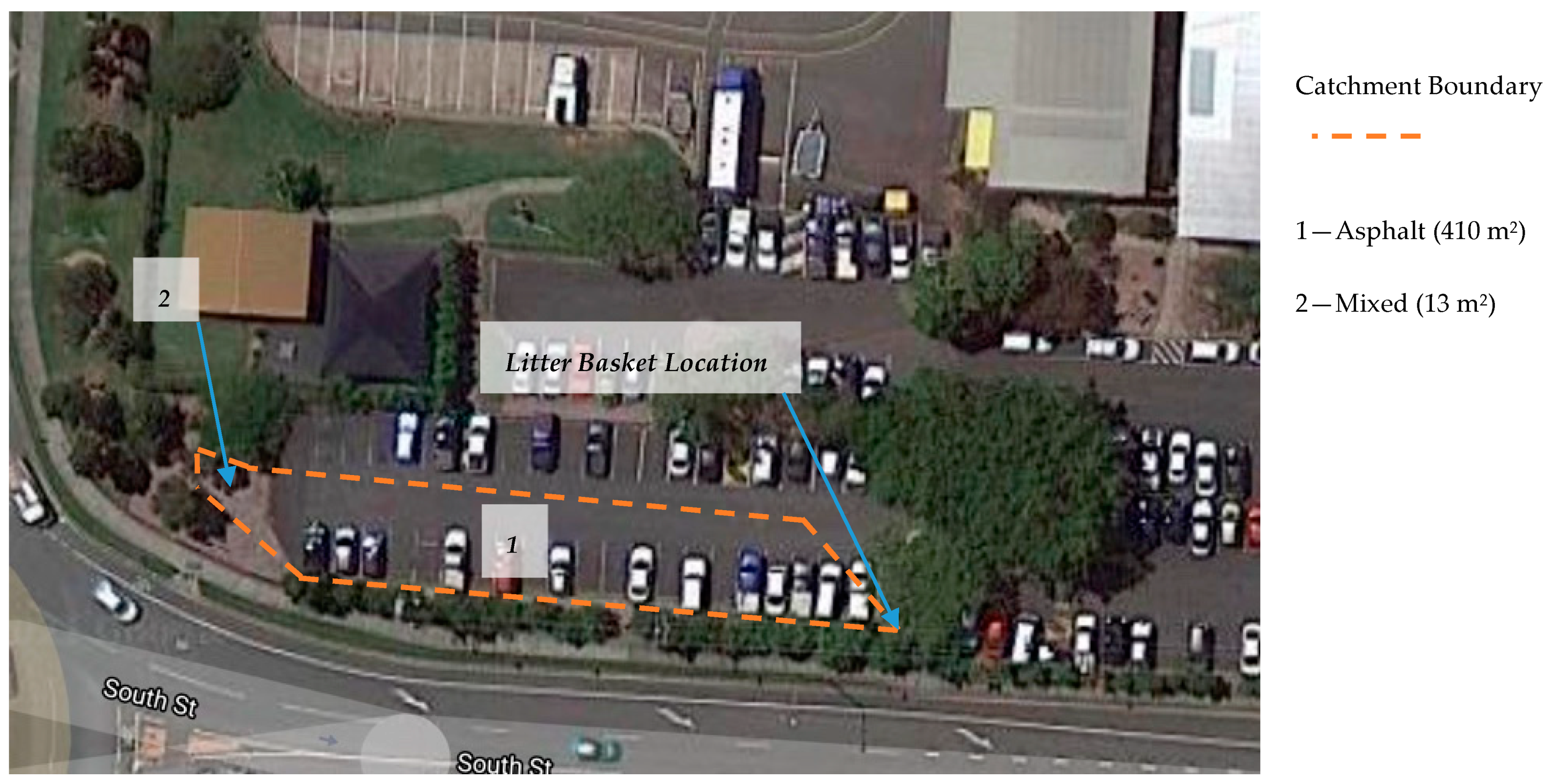
The test site, located in Thornlands, Queensland, Australia, was identified to install the Ecosol Litter Basket for monitoring and testing. The location of the unit was selected based on the National Institute of Water and Atmospheric Research Ltd. (NIWA) guidelines [16] as detailed in Figure 1.

The site is a part of the Redland City Council Depot, where the catchment area of the selected site is almost 423 m² and is predominately road and pavement, with 90% being impervious. Preliminary sampling was taken for water quality testing to characterize the trial site to avoid a site where pollutant concentrations were likely to fall outside the limits allowed for qualifying events, or where pollutant concentrations fall below laboratory limits of detection (LOD) [1].

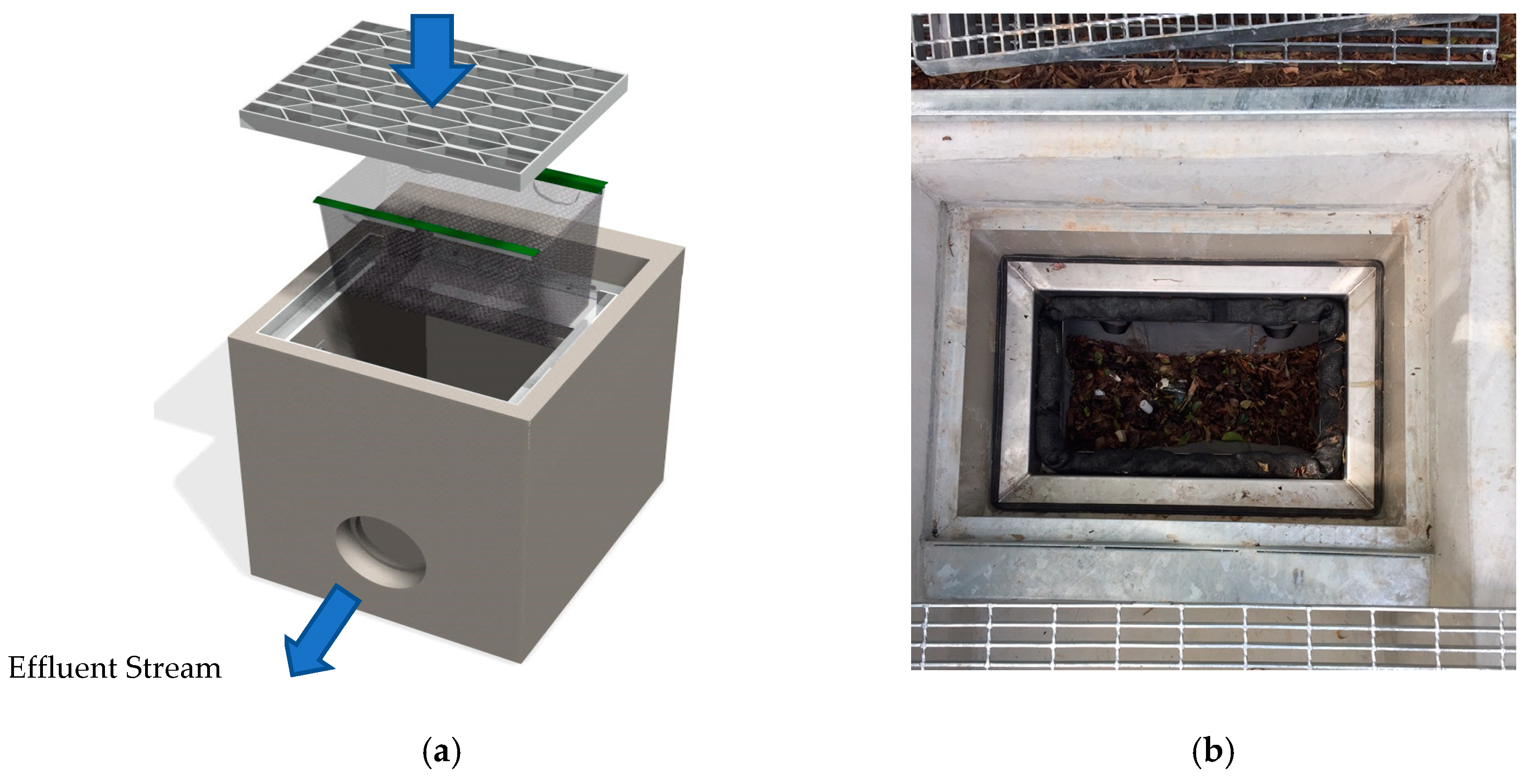
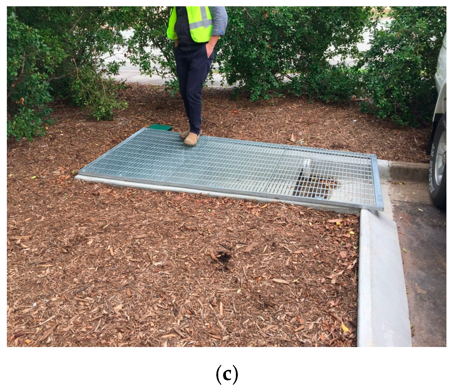
The Ecosol Litter Basket captures pollutants conveyed by rainfall runoff at drainage entry points (at-source) and consists of a stainless-steel frame and removable filtration basket with a 200 μm mesh. It was designed as a primary treatment measure. For the testing unit installed at the test site, the treatable flow rate was estimated to be 22 L/s [2]. Figure 2 shows the installed device.

2.2. Instrumentation and Sampling Methodology

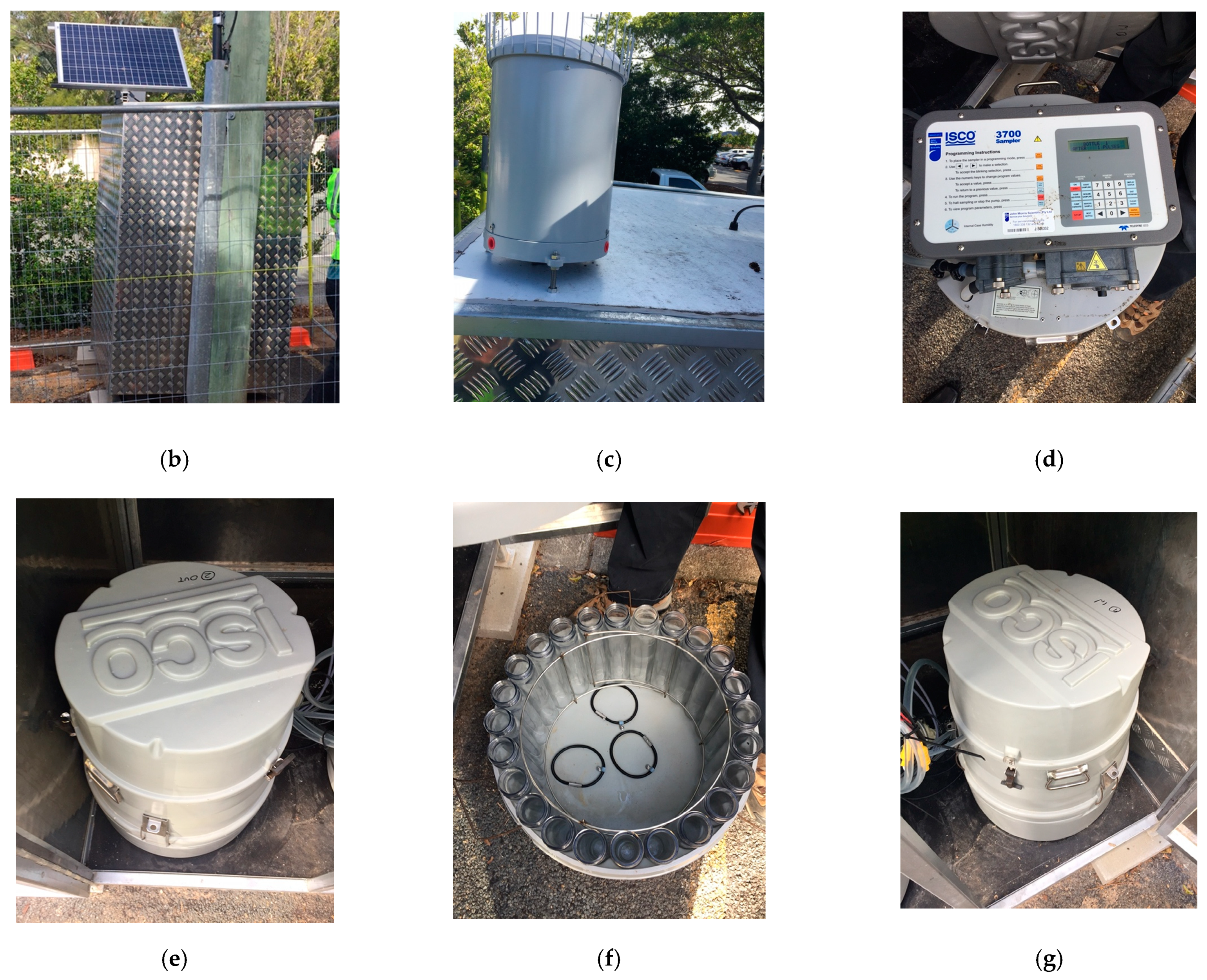
Sampling was undertaken by two Isco 3700 Full-size autosamplers (24 $\times$ 250 mL) for the influent and effluent streams during each rainfall. The pump rate of the Isco 3700 autosampler is 3000 mL/min with a line transport velocity of 0.70 m/s through a medical-grade sample tube (3/8” inner diameter). For continuous depth measurement, pressure sensing LMP 307 stainless steel probes were used. A rain gauge (Model TB3) which was compatible with the requirements of [1] (sampling at intervals of 5 min and increments of 0.2 < 0.25 mm), was used for measuring rainfall. The data logger Model CR1000 was used for collecting the signals from the sensing instruments. The installed instrumentation is shown in Figure 3.

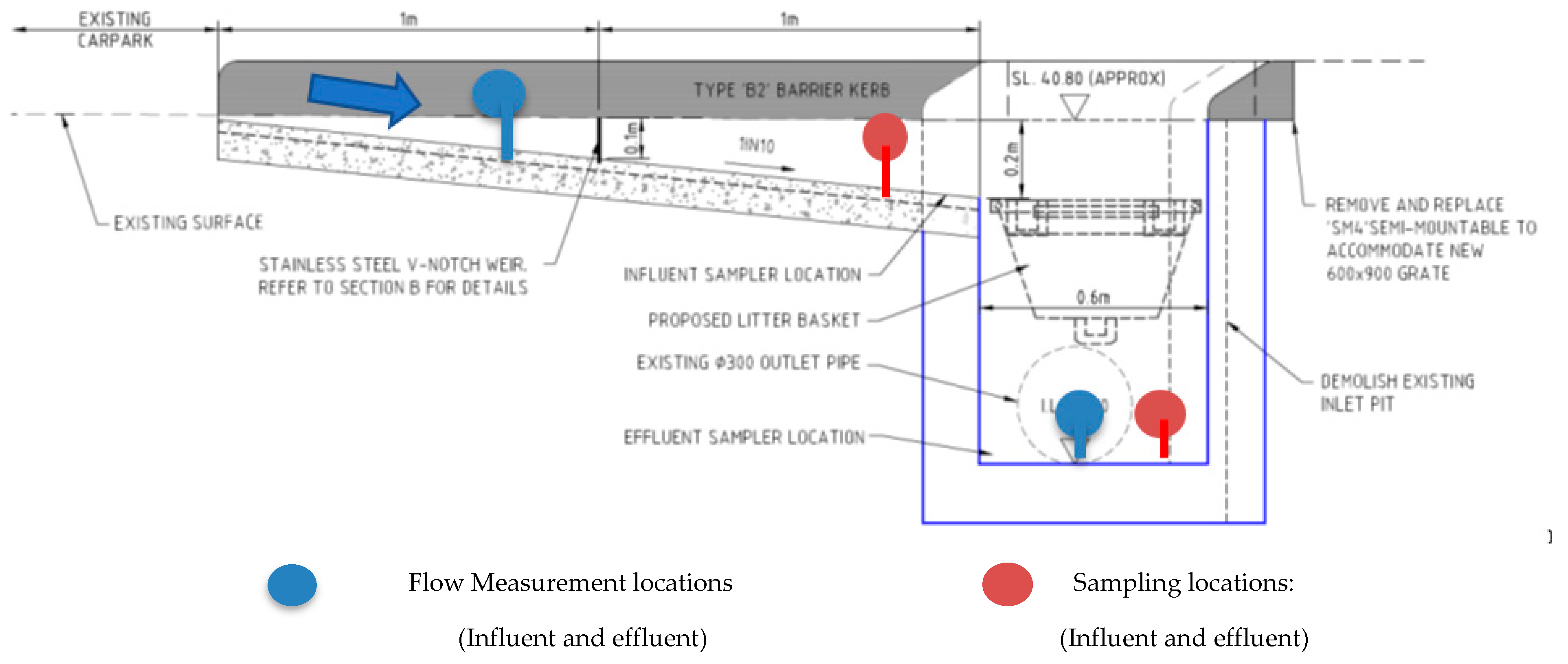
The adopted sampling methodology was selected based on the methodology discussed in [18]. Grab samples (a maximum of four samples at 2 min intervals at the start of each event) were used to evaluate event mean concentration (EMC) for total petroleum hydrocarbons (TPH) and total recoverable hydrocarbons (TRH). Following this, for composite samples, the volumetric intervals between the first 8 aliquots were selected to be 750 L. After collecting 8 aliquots, the volumetric sampling interval increased to 3000 L. Composite samples were used to evaluate event mean concentration (EMC) for TSS, TP, TN, and heavy metals. The locations of the sampling for influent and effluent streams are shown in Figure 4.

2.3. Overview of Metrics

The removal efficiency metrics (suggested by [1]) that are generally used for evaluating the performance of a stormwater filtration device along with regression metrics are comprehensively discussed in [18] and are summarized in

Table 1. Summary of the removal efficiencies.

Metrics		Equation	Equation No.
Efficiency Metrics	Concentration Removal Efficiency (CRE)	$CRE=\frac{EM{C}_{in}-EM{C}_{out}}{EM{C}_{in}},$	(1)
	Efficiency Ratio (ER)	$ER=1-\frac{average outlet EMC}{average inlet EMC} ,$	(2)
		$average EMC=\frac{{{\displaystyle \sum }}_{j=1}^{m}EM{C}_j}{m},$	(3)
	Summation of Loads (SOL)	$SOL=1-\frac{Sum of outlet loads}{Sum of inlet loads} ,$	(4)
		$Sum of loads={{\displaystyle \sum }}_{j=1}^{m}EM{C}_{j }{V}_j ,$	(5)
	Efficiency of Individual Storm Loads (ISL)	$Individual Storm Efficiency=1-\frac{Load{ }_{out}}{Loa{d}_{in}} ,$	(6)
		$Average Efficiency=\frac{{{\displaystyle \sum }}_{j=1}^{m}Storm Efficienc{y}_j}{m},$	(7)
Regression Metrics	Regression of Loads (ROL)	$ROL=1-\frac{2}{{\overline{x}}^2}{{\displaystyle \int }}_0^{\overline{x}}f\left(x\right)dx,$	(8)
	Regression of Concentrations (ROC)	$ROC=1-\frac{2}{{\overline{x}}^2}{{\displaystyle \int }}_0^{\overline{x}}f\left(x\right)dx,$	(9)

. The results of these two metric categories (efficiency and regression metrics) are presented and will be compared in Section 3.

With reference to Table 1:

$EM{C}_{in }$ and $EM{C}_{out}$ are the influent and effluent event mean concentrations respectively;

m is the number of storm events;

$V_j$ is the total volume of flow for storm event j;

$f\left(x\right)$ in Equation (8) is the nonlinear regression curve of the inlet loads with respect to outlet loads;

$f\left(x\right)$ in Equation (9) is the nonlinear regression curve of event mean concentration influent with respect to event mean concentration effluent; and

$\overline{x}$ is the centroid of the area under the fitting curve.

To evaluate the fitting curve for both of the regression metrics, both the squared correlation $\left(R^2\right)$ and the root mean squared error (RMSE) are calculated, as below:

$$RMSE=\sqrt{\frac{{\sum }_{i=1}^n{\left({\tilde{y}}_i-y_i\right)}^2}{n},}$$

(10)

$$R^2=1-\frac{{\sum }_{i=1}^n{\left({\tilde{y}}_i-y_i\right)}^2}{{\sum }_{i=1}^n{\left(y_i-\mu \right)}^2} ,$$

(11)

where $y_i$ and ${\tilde{y}}_i$ are the measured and predicted outputs respectively (loading for ROL and event mean concentration for ROC), and $\mu$ is the average of the measured output.

2.4. Confidence Level

In accordance with [1], to achieve statistical confidence for the performance of the stormwater device, event mean concentration with relatively consistent concentrations and removal efficiencies may be required. In cases where the concentrations and removal efficiencies are more highly varied, additional samples are needed to account for the variability. The goal of testing is to satisfy the 90% statistical significance where practical to do so.

3. Results

The two key criteria for accepting a rainfall event as a qualifying event are based on the hydraulic properties of the run-off (i.e., duration, and the interval between events) and the input pollutant concentration values (i.e., concentrations within an acceptable band) [1]. These are comprehensively discussed in [18].

Between May 2017 and March 2019, a total number of 29 rainfall events occurred.

Table A1. Event details.

Events	Date/Time			Antecedent Dry Period (ADP) (h)	Rain Depth (mm)	Number of Aliquots	Maximum Intensity (mm/h)	Peak Flow Rate (L/s)		Qualifying Events? (Based on Hydraulic Criteria) (Y/N)
	Start	End	Duration (h)					Influent	Effluent
Rainfall 1	18/5/17 23:48	Sampler did not reach 8 aliquots, samples not sent to the lab								N
Rainfall 2	10/6/17 19:46	11/6/17 12:00	16.23	523.80	19.4	8	36	1.87	1.87	Y
Rainfall 3	15/7/17 18:28	16/7/17 9:00	14.53	822.47	26.2	11	66	5.47	5.24	Y
Rainfall 4	18/11/17 11:00	19/11/17 17:00	30.00	3002.00	30.2	12	72	9.59	5.69	Y
Rainfall 5	20/11/17 22:00	22/11/17 14:00	40.00	29.00	14.8	8	120	7.39	6.82	Y
Rainfall 6	29/11/17 5:00	Broken inlet aliquot jar remaining samples deemed to not be representative of the event								N
Rainfall 7	4/12/17 12:00	4/12/17 20:04	8.07	72.57	21.2	20	24	2.6	1.48	Y
Rainfall 8	25/12/2017	Sampler did not reach 8 aliquots, samples not sent to the lab								N
Rainfall 9	2/1/2018	Sampler did not trigger properly								N
Rainfall 10	1/2/18 19:12	3/2/18 16:34	45.37	717.20	37	10	36	1.84	1.72	Y
Rainfall 11	11/2/18 18:20	11/2/18 20:00	1.67	193.77	46.4	10	204	32	20.1	Y
Rainfall 12	22/2/18 15:52	23/2/18 5:54	14.03	259.87	59.6	16	54	4.4	4.05	Y
Rainfall 13	26/2/18 19:44	Aliquot volumes were not equal and deemed not representative of the event								N
Rainfall 14	6/3/18 4:20	Sampler did not reach 8 aliquots, samples not sent to the lab								N
Rainfall 15	21/3/18 0:50	21/3/18 4:45	3.92	356.50	16.8	8	48	8.4	5.3	Y
Rainfall 16	22/3/18 20:00	22/3/18 22:20	2.33	39.25	18.4	10	72	6.4	4.2	Y
Rainfall 17	26/8/18 0:00	26/8/18 12:32	12.53	3745.67	28	12	48	5.8	5.8	Y
Rainfall 18	4/9/18 13:20	5/9/18 7:32	18.20	216.80	51.8	22	102	10.05	10.05	Y
Rainfall 19	11/10/18 12:30	11/10/18 13:50	1.33	868.97	8.4	6	30	2.54	2.54	Y
Rainfall 20	12/10/18 18:26	13/10/18 5:00	10.57	28.60	13.6	6	24	2.26	2.26	Y
Rainfall 21	13/10/18 9:56	13/10/18 22:06	12.17	4.93	25.4	13	24	2.23	2.23	Y
Rainfall 22	21/10/18 14:30	21/10/18 20:56	6.43	184.4	15	7	72	8.8	8.8	Y
Rainfall 23	5/12/18 11:14	5/12/18 13:30	2.27	1070.3	15	9	54	5.0	5.0	Y
Rainfall 24	16/12/18 12:52	16/12/18 21:40	8.80	263.37	21.2	14	36	2.7	2.7	Y
Rainfall 25	Sampler didn’t reach 8 aliquots, samples not sent to the lab								N
Rainfall 26	4/2/19 6:45	4/2/19 9:08	2.38	2737.7	9.2	6	30	2.17	2.17	Y
Rainfall 27	5/2/19 21:56	6/2/19 3:44	5.80	2759.8	24.4	15	66	6	6	Y
Rainfall 28	7/2/19 2:18	7/2/19 5:04	2.77	22.57	9.6	7	48	2.96	2.96	Y
Rainfall 29	14/3/19 20:38	14/3/19 21:20	0.70	855.57	21.2	5	150	17.04	17.04	Y

(in Appendix A) shows the recorded details of each event during the field test. It can be seen that a wide range of storm behaviors, and consequent flow rates were covered by the events. The total number of events for qualifying for each pollutant type is as follows: 15 for TSS, TN, and THM; 16 for TP; and 13 for TPH and TRH. Based on the sampling methodology, the event mean concentrations (EMCs) were determined by an independent NATA accredited laboratory analysis for both grab samples and the flow-weighted composites of aliquots.

Table 2. Qualifying event details for total suspended solids (TSS) (LOD = 5 mg/L).

Qualifying Event No	Rainfall Event No	Number of Aliquots	Max Flowrate (L/s)	Flow Volume (L)	TSS (mg/L)
					Influent	Effluent
1	Rainfall 2	8	1.87	5833	51.65	35.87
2	Rainfall 4	12	5.69	1405	32.00	19.00
3	Rainfall 5	8	6.82	2261	52.00	2.500
4	Rainfall 10	10	1.84	5492	38.00	2.500
5	Rainfall 11	10	32.0	17,746	42.00	13.00
6	Rainfall 12	16	4.40	14,151	142.0	92.00
7	Rainfall 17	12	5.80	9783	75.00	6.000
8	Rainfall 19	6	2.54	3085	22.00	12.00
9	Rainfall 20	6	2.26	3950	49.00	11.00
10	Rainfall 21	13	2.23	9549	6.000	2.500
11	Rainfall 22	7	8.80	4780	6.000	7.000
12	Rainfall 23	9	5.00	5096	42.00	14.00
13	Rainfall 24	14	2.70	7145	19.00	8.000
14	Rainfall 26	6	2.17	3155	35.00	11.00
15	Rainfall 29	5	17.04	7380	16.00	2.500

and

Table A2. Qualifying events details for total phosphorus (TP) (LOD = 0.01 mg/L).

Qualifying Event No	Rainfall No	Number of Aliquots	Max Flowrate (L/s)	Flow Volume (L)	TP (mg/L)
					Influent	Effluent
1	Rainfall 2	8	1.87	5833	0.056	0.031
2	Rainfall 4	12	5.69	1405	0.060	0.060
3	Rainfall 5	8	6.82	2261	0.160	0.030
4	Rainfall 10	10	1.84	5492	0.210	0.080
5	Rainfall 11	10	32.0	17,746	0.090	0.070
6	Rainfall 12	16	4.40	14,151	0.320	0.220
7	Rainfall 17	12	5.80	9783	0.120	0.090
8	Rainfall 18	22	10.05	17,537	0.020	0.040
9	Rainfall 19	6	2.54	3085	0.030	0.040
10	Rainfall 20	6	2.26	3950	0.050	0.020
11	Rainfall 21	13	2.23	9549	0.030	0.020
12	Rainfall 22	7	8.80	4780	0.020	0.010
13	Rainfall 23	9	5.00	5096	0.050	0.040
14	Rainfall 24	14	2.70	7145	0.010	0.010
15	Rainfall 26	6	2.17	3155	0.030	0.030
16	Rainfall 29	5	17.04	7380	0.110	0.030

,

Table A3. Qualifying events details for total nitrogen (TN) (LOD = 0.1 mg/L).

Qualifying Event No	Rainfall No	Number of Aliquots	Max Flowrate (L/s)	Flow Volume (L)	TN (mg/L)
					Influent	Effluent
1	Rainfall 2	8	1.87	5833	0.634	0.508
2	Rainfall 4	12	5.69	1405	0.400	1.000
3	Rainfall 5	8	6.82	2261	3.800	0.600
4	Rainfall 11	10	32.0	17,746	2.000	2.400
5	Rainfall 12	16	4.40	14,151	2.800	1.800
6	Rainfall 17	12	5.80	9783	1.400	1.100
7	Rainfall 18	22	10.05	17,537	0.200	0.100
8	Rainfall 19	6	2.54	3085	0.400	1.100
9	Rainfall 20	6	2.26	3950	0.400	0.100
10	Rainfall 21	13	2.23	9549	0.100	0.050
11	Rainfall 22	7	8.80	4780	0.100	0.100
12	Rainfall 23	9	5.00	5096	0.600	0.400
13	Rainfall 24	14	2.70	7145	0.300	1.300
14	Rainfall 26	6	2.17	3155	0.300	1.300
15	Rainfall 29	5	17.04	7380	1.200	0.400

,

Table A4. Qualifying events details for total heavy metals (THM) (LOD not available).

Qualifying Event No	Rainfall No	Number of Aliquots	Max Flowrate (L/s)	Flow Volume (L)	THM (µg/L)
					Influent	Effluent
1	Rainfall 2	8	1.87	5833	57.32	87.98
2	Rainfall 4	12	5.69	1405	26.87	36.10
3	Rainfall 5	8	6.82	2261	454.2	31.55
4	Rainfall 10	10	1.84	5492	66.26	284.7
5	Rainfall 11	10	32.0	17,746	78.11	165.8
6	Rainfall 12	16	4.40	14,151	164.4	157.4
7	Rainfall 17	12	5.80	9783	143.0	69.00
8	Rainfall 18	22	10.05	17,537	22.00	28.00
9	Rainfall 19	6	2.54	3085	39.00	35.00
10	Rainfall 20	6	2.26	3950	55.00	18.50
11	Rainfall 21	13	2.23	9549	14.00	21.00
12	Rainfall 22	7	8.80	4780	21.00	20.00
13	Rainfall 23	9	5.00	5096	54.00	47.00
14	Rainfall 24	14	2.70	7145	33.00	13.00
15	Rainfall 26	6	2.17	3155	36.00	22.50

,

Table A5. Qualifying events details for total petroleum hydrocarbons (TPH) (LOD = 50 µg/L).

Qualifying Event No	Rainfall No	Max Flowrate (L/s)	Flow Volume (L)	TPH (µg/L)
				Influent	Effluent
1	Rainfall 2	1.87	5833	3089	1738
2	Rainfall 7	2.60	5785	1096	946.2
3	Rainfall 10	1.84	5492	2512	1016
4	Rainfall 12	4.40	14,151	3816	3695
5	Rainfall 17	5.80	9783	820.0	220.0
6	Rainfall 19	2.54	3085	240.0	50.00
7	Rainfall 20	2.26	3950	292.5	196.7
8	Rainfall 22	8.80	4780	482.4	290.1
9	Rainfall 23	5.00	5096	672.6	590.2
10	Rainfall 24	2.70	7145	267.3	25.00
11	Rainfall 26	2.17	3155	424.1	177.3
12	Rainfall 27	6.00	9466	198.1	25.00
13	Rainfall 28	2.96	3763	123.6	25.00

and

Table A6. Qualifying events details for total recoverable hydrocarbons (TRH) (LOD = 100 µg/L)

Qualifying Event No	Rainfall No	Max Flowrate (L/s)	Flow Volume (L)	TRH (µg/L)
				Influent	Effluent
1	Rainfall 2	1.87	5833	3677	2013
2	Rainfall 7	2.60	5785	1175	893.4
3	Rainfall 10	1.84	5492	2694	1060
4	Rainfall 12	4.40	14,151	3947	3952
5	Rainfall 17	5.80	9783	930.0	160.0
6	Rainfall 19	2.54	3085	200.0	110.0
7	Rainfall 20	2.26	3950	250.0	152.5
8	Rainfall 22	8.80	4780	532.2	248.9
9	Rainfall 23	5.00	5096	664.6	571.2
10	Rainfall 24	2.70	7145	294.8	50.00
11	Rainfall 26	2.17	3155	397.9	191.5
12	Rainfall 27	6.00	9466	175.3	50.00
13	Rainfall 28	2.96	3763	120.6	50.00

show the ECM results for all pollutant types for both the influent and effluent streams. In accordance with [1], effluent event mean concentrations less than the limit of detection (LOD) (reported by the laboratory) were set at half of the LOD. As observed in Table 2, the qualifying events cover a broad range of flow conditions from 1.84 L/s (total storm volume of approximately 5 kL) up to 32 L/s (total storm volume of above 17 kL), and influent TSS concentrations (from 6 mg/L up to 142 mg/L).

3.1. Statistical Analysis

A statistical analysis of the event mean concentration dataset is required for evaluating the performance of the stormwater filtration device. Within this section, firstly, data visualizations are presented, followed by an analysis of the influent and effluent distributions to determine the significance of the device on filtering the pollutant constituents.

3.1.1. Data Summary Plots

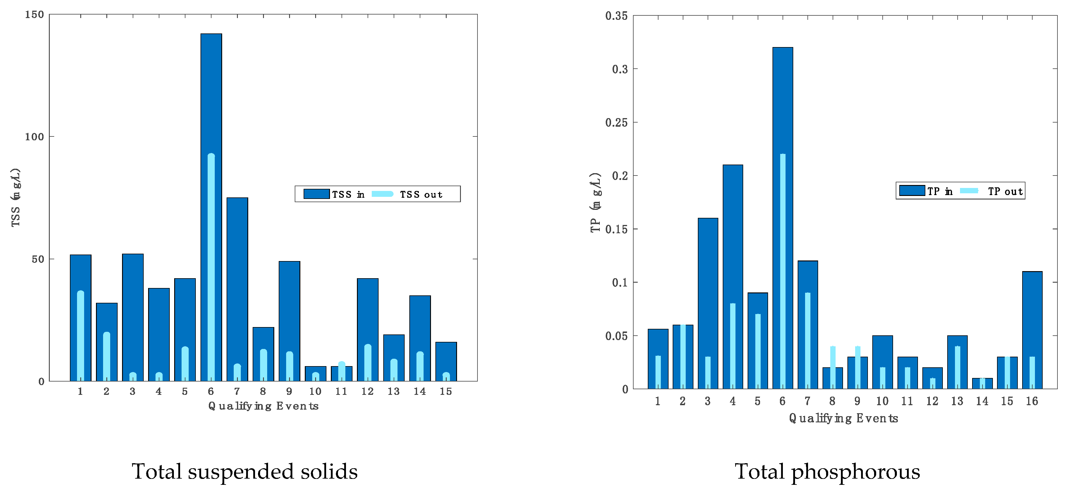
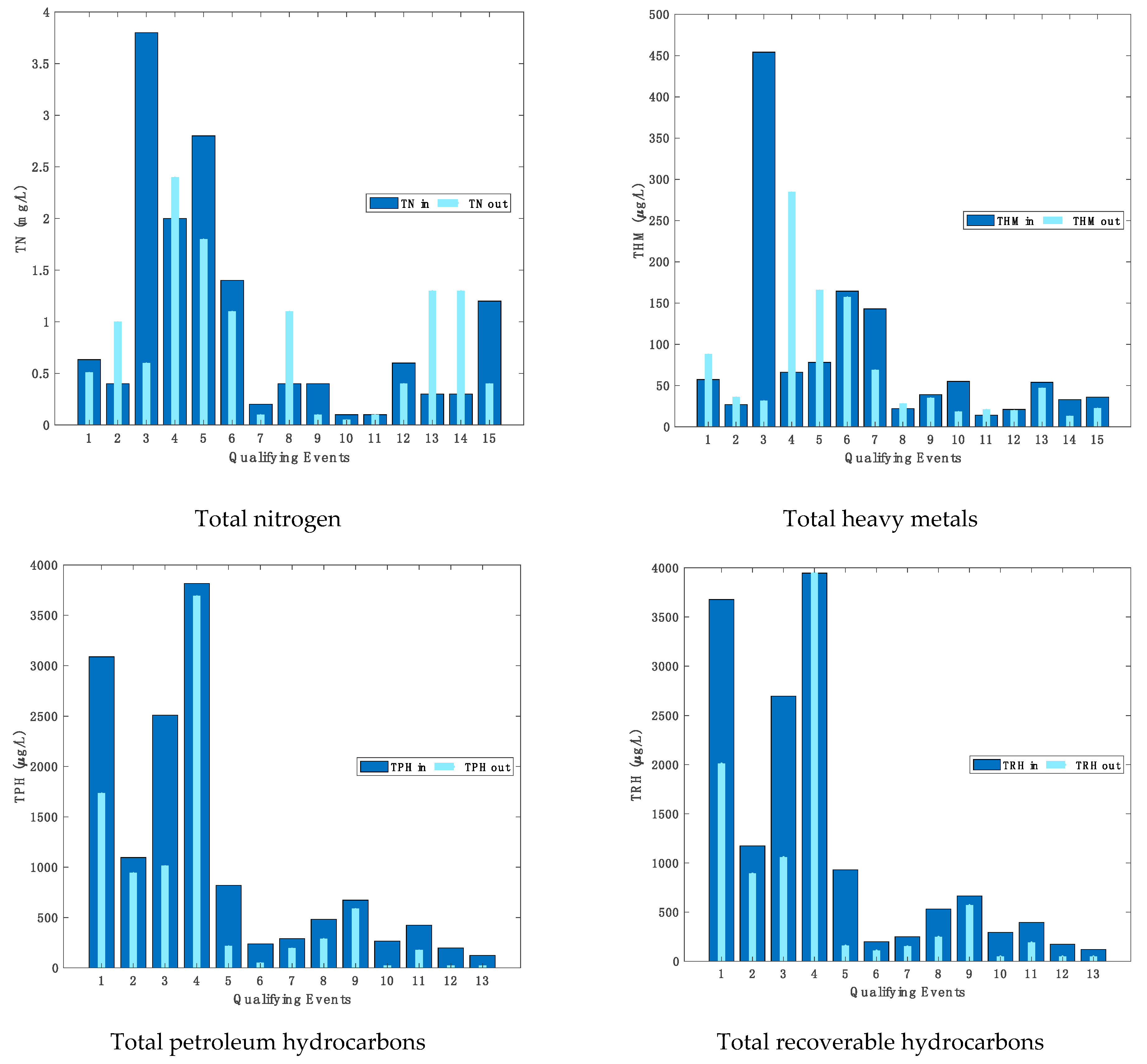
To provide an overview of the qualifying event data, Figure 5 provides interleaved bar plots of a direct comparison between the relative magnitude of the ECMs from the influent and the effluent streams. With regards to TSS, it is relatively clear that the effluent stream has reduced TSS concentration in comparison to the influent stream, particularly events 3, 4 and 7. Event 11 yielded anomalous results with the effluent marginally higher in TSS than the influent, which is attributed to the very low influent concentration and potential measurement errors. The results are less conclusive for the other pollutant types, with generally high relative effluent concentrations (as for TP, TPH and TRH), and even many cases where a higher effluent concentration was regularly recorded (as for TN and THM).

To reinforce the message from Figure 5 and Figure 6 shows the box and whisker plots for influent and effluent ECMs of all pollutants (notches indicate the 95% confidence interval). As observed in this figure, all data are highly skewed towards the lower concentrations. Overlapping confidence intervals between the influent and effluent box plots indicate that the central tendency of the data may not be significantly different [18]. A significant difference in the central tendency of the influent and effluent streams (with the effluent being the lesser of the two) is a key indicator that the filtration device is effective in reducing pollutant concentrations. From the box plots, it is observed that only the TSS medians are clearly different, indicating the effectiveness of the device in filtering TSS. This is discussed in more detail in the following section. It is also noted that the variability in the data is quite high, and that the influent data typically have much higher variability than the effluent data, except for the case of TP.

3.1.2. Influent and Effluent Distributions, and Significance

In order to assess the significance in the difference between the influent and effluent streams (and the implied effectiveness of the device), first, the influent and effluent distributions need to be determined, followed by the use of an appropriate statistical significance test.

Table 3. Descriptive Statistics and distribution results of the datasets.

Descriptive Statistics	TSS (mg/L)		TP (mg/L)		TN (mg/L)		THM (µg/L)		TPH (µg/L)		TRH (µg/L)
	Influent	Effluent	Influent	Effluent	Influent	Effluent	Influent	Effluent	Influent	Effluent	Influent	Effluent
Median	31.16	9.03	0.0567	0.0373	0.5576	0.4886	53.12	44.53	611.8	234.1	616.90	281.23
Mean	44.96	15.53	0.0888	0.0513	1.0393	1.0287	79.88	67.92	1120.0	971.0	1226.0	801.77
Std. Deviation	46.75	21.72	0.1069	0.0485	1.6345	1.9062	89.70	78.20	1720.0	3909.1	2105.7	2140.6
Std. Error of Mean	12.07	5.607	0.0267	0.0121	0.4220	0.4922	23.16	20.19	477.04	1084.2	584.02	593.70
Coefficient of variation	104%	140%	120%	94.0%	157%	185%	112%	115%	153%	403%	172%	267%
Likely distribution	Lognormal	Lognormal	Lognormal	Lognormal	Lognormal	Lognormal	Lognormal	Lognormal	Lognormal	Lognormal	Lognormal	Lognormal

shows the descriptive statistics and distributional analysis results of the influent and effluent ECM data. The high coefficient of variation shows the high variability in the measurements, and it is observed that all sampled streams and ECMs were found to be lognormally distributed (

Table A7. Normality test results for event mean concentrations (EMCs).

Tabular results	TSS		TP		TN		THM		TPH		TRH
	Influent	Effluent	Influent	Effluent	Influent	Effluent	Influent	Effluent	Influent	Effluent	Influent	Effluent
Test for normal distribution
Shapiro–Wilk test
W	0.8110	0.5827	0.7996	0.6896	0.7697	0.9070	0.5965	0.7200	0.7494	0.6860	0.7392	0.6645
p value	0.0051	<0.0001	0.0027	0.0001	0.0015	0.1217	<0.0001	0.0004	0.0018	0.0004	0.0014	0.0003
Passed normality test?	No	No	No	No	No	Yes	No	No	No	No	No	No
p value summary	**	***	**	***	**	ns	***	***	**	***	**	***
Anderson–Darling test
A2*	0.8854	2.337	1.161	1.640	1.407	0.4881	2.246	1.695	1.445	1.539	1.480	1.729
p value	0.0175	<0.0001	0.0034	0.0002	0.0008	0.1891	<0.0001	0.0001	0.0006	0.0003	0.0004	<0.0001
Passed normality test?	No	No	No	No	No	Yes	No	No	No	No	No	No
p value summary	*	***	**	***	***	ns	***	***	***	***	***	***
Test for lognormal distribution
Shapiro–Wilk test
W	0.9284	0.9184	0.9811	0.9597	0.9571	0.8977	0.9475	0.9222	0.9406	0.9303	0.9352	0.9292
p value	0.2582	0.1823	0.9719	0.6568	0.6423	0.0877	0.4859	0.2081	0.4644	0.3443	0.3976	0.3327
Passed normality test?	Yes	Yes	Yes	Yes	Yes	Yes	Yes	Yes	Yes	Yes	Yes	Yes
p value summary	ns	ns	ns	ns	ns	ns	ns	ns	ns	ns	ns	ns
Anderson–Darling test
A2*	0.5127	0.4563	0.1778	0.3089	0.2620	0.6760	0.3235	0.5002	0.3190	0.3370	0.3051	0.3410
p value	0.1628	0.2289	0.9032	0.5211	0.6521	0.0616	0.4907	0.1757	0.4939	0.4464	0.5199	0.4364
Passed normality test?	Yes	Yes	Yes	Yes	Yes	Yes	Yes	Yes	Yes	Yes	Yes	Yes
p value summary	ns	ns	ns	ns	ns	ns	ns	ns	ns	ns	ns	ns

ns—Not significant; * Significant; ** Very significant; *** Extremely significant.

in Appendix B).

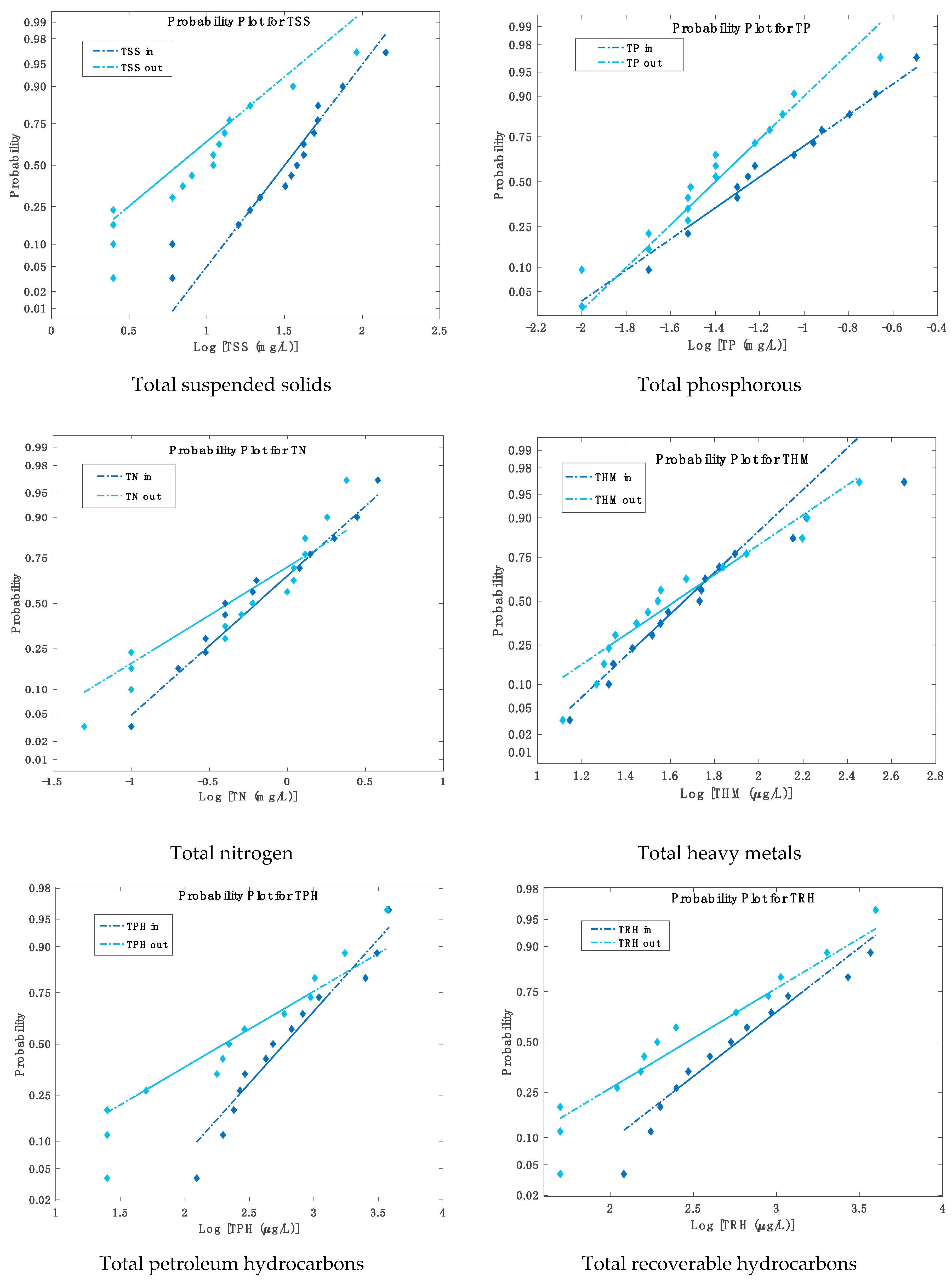
To better visualize the distributions, a comparison of the ECMs for the influent and effluent streams’ cumulative probability plots for all paired datasets is shown in Figure 7. A visual consideration of Figure 7 indicates that only the TSS the influent and effluent distributions are clearly distinct from one another, which indicates that a meaningful reduction of TSS does occur from the influent to the effluent stream. For all other constituents, the difference between the influent and effluent streams is far less pronounced, as the regression lines for the influent and effluent streams are either very close, or even cross over one another.

With regards to the significance testing of the influent and effluent EMCs, as the data are lognormally distributed, the validity of the paired t-Test holds and is suitable for use (

Table 4. Statistical significance test results—Paired Samples t-Test.

Constituents	Unit	Paired Differences					t	p-Value(Two-Tailed)	Significantly Different(p < 0.05)?
		Mean	Std. Deviation	Std. Error Mean	95% CI 1 of the Difference
					Lower	Upper
TSS in—TSS out	mg/L	25.92	19.59	5.059	15.07	36.77	5.123	0.0002	Yes ***
TP in—TP out	mg/L	0.0341	0.0485	0.0121	0.0082	0.0599	2.810	0.0132	Yes *
TN in—TN out	mg/L	0.1584	1.027	0.2651	−0.4103	0.7271	0.5974	0.5598	No (ns)
THM in—THM out	μg/L	15.11	130.7	33.75	−57.28	87.50	0.4478	0.6611	No (ns)
TPH in—TPH out	μg/L	387.5	479.0	132.8	98.12	677.0	2.917	0.0129	Yes *
TRH in—TRH out	μg/L	427.3	574.8	159.4	79.99	774.7	2.681	0.0200	Yes *

* Significant; *** Extremely significant. “ns” means not significant. ¹ Confidence Interval.

).

From the t-Test results, it can be seen that the influent and effluent EMCs for TSS, TP, TPH, and TRH are significantly different in their means with a 95% confidence. Further, the difference in the TSS ECMs was observed to be extremely significant with a p-value of 0.0002. This means that the Ecsosol Litter Basket is observed to remove fractions of these pollutant types. The results for TN and THM indicate no significant changes between the influent and effluent EMCs.

From the results of the nonparametric test, it is observed that the influent and effluent stream EMCs for constituents TSS, TP, TPH, and TRH are significantly different in their medians. The TSS differences in EMC from influent to effluent are considered extremely significant (with a p-value of 0.0002), where whereas the differences for TP, TPH and TRH are just classed as significant (with p-values on the order of 10⁻²). The results for TN and THM show no significant changes between the influent and effluent EMCs (with p-values in excess of 0.5). These results confirm the observations from the data visualizations in Figure 5, Figure 6 and Figure 7. The interpretation of this result is that only the performance metric results for TSS, TP, TPH and TRH in the following section are considered statistically significant. For completeness, nonparametric tests (Sign Test and Wilcoxon–Mann–Whitney Rank-Sign Test) are used for comparison, and were found to support the conclusions of the t-Test.

3.2. Performance Metrics Evaluation

As discussed in Section 2.3, for evaluating the performance efficiency of a stormwater filtration device, a range of pollutant removal metrics have been utilized in monitoring studies. In this section, the performance metrics for the Ecosol Litter Basket filtration of each pollutant type will be presented. The results for TN and THM were included for the sake of completeness (despite not being statistically significant).

3.2.1. Efficiency Metrics

Statistical parameters for the performance metrics, such as mean, median, standard deviation, coefficient of variation (CV), and confidence level are shown in

Table 5. Statistical parameters for performance metrics.

Pollutant	Metrics	Mean	Median	ST DEV	CV	Confidence Level (EMCin, EMCout)
TSS	CRE	59.9%	66.7%	29.8%	49.8%	93%
	Storm Efficiency	59.9%	66.7%	29.8%	49.8%
TP	CRE	23.1%	28.1%	44.7%	194%	69%
	Storm Efficiency	23.1%	28.1%	44.7%	194%
TN	CRE	−38.4%	21.4%	141%	−368%	27%
	Storm Efficiency	−38.4%	21.4%	141%	−368%
THM	CRE	−17.7%	4.8%	102%	−575%	25%
	Storm Efficiency	−17.7%	4.8%	102%	−575%
TPH	CRE	51.8%	58.2%	30.0%	58.0%	46%
	Storm Efficiency	51.8%	58.2%	30.0%	58.0%
TRH	CRE	48.4%	51.9%	24.9%	51.5%	47%
	Storm Efficiency	48.4%	51.9%	24.9%	51.5%

. It can be seen that the mean value for TN and THM is highly negative, which can explain the results of the significance testing as discussed in Section 3.1.2, namely, the results for these pollutant types is highly variable, leading to a lack of significance in the results. The CV for all significant pollutant types is also very high, being around 50% for TSS, TPH and TRH, up to almost 200% for TP. This degree of variability in the results is typical for field studies of stormwater filtration devices.

From Table 5, it is also noted that the confidence level for all pollutants, except TSS, is less than 90%. This means that despite all TSS, TP, TPH and TRH being evaluated as having significantly different influent and effluent ECMs, it is only TSS that provides high confidence in the performance metric values (classed in [1] as being greater than 90%).

3.2.2. Regression Metrics

Regression metrics include the regression of loads (ROL) and the regression of concentrations (ROC), as shown in Table 1 and comprehensively discussed in [18]. The best regression curves, along with their functions ($f\left(x\right))$ for all pollutants loads, are shown in Figure 8. It is observed that the regression curve is linear only for TN, whereas for the other pollutant loads the regression curves are not linear, meaning that the influent–effluent relationship for these pollutant types is nonlinear.

Table 6. Regression of loads results.

Pollutant	Average of Loads (grams)		Range of Influent Loads (grams)	$\overline{\mathit{x} }{ }^1$ (grams)	R Squared	RMSE (grams)	$\frac{\mathbf{R}\mathbf{M}\mathbf{S}\mathbf{E}}{\left(\mathbf{A}\mathbf{v}\mathbf{e}\mathbf{r}\mathbf{a}\mathbf{g}\mathbf{e} \mathbf{o}\mathbf{f} \mathbf{E}\mathbf{M}\mathbf{C} \mathbf{o}\mathbf{u}\mathbf{t}\right)}$	ROL
	Load in	Load out
TSS	339.1	144.4	0.0–2009.0	1478	0.963	61.00	42%	65%
TP	0.718	0.484	0.0–4.53	3.045	0.945	0.178	37%	35%
TN	8.295	7.295	0.0–39.6	26.67	0.816	4.861	67%	14%
THM	0.564	0.628	0.0–2.33	1.511	0.529	0.595	95%	−12%
TPH	8.722	6.310	0.0–54.0	38.46	0.994	1.092	17%	36%
TRH	9.308	6.684	0.0–55.9	39.82	0.994	1.118	17%	39%

¹ Centroid of the area under the fitting curve.

shows a summary of the fitting curves along with the values of $RMSE$, $R^2$, and ROL. The ROL efficiency for each pollutant was calculated based on Equation (8) at $x=\overline{x},$ where $\overline{x}$ is the centroid of the area under the fitting curve. The low value of ROL for TN and THM is notable which is 14% and −12% respectively. It is also noted that the maximum ROL (65%) was achieved for TSS.

The best regression fitting curves for all event mean concentrations (EMCs) along with their functions (f(x) are shown in Figure 9. It can be seen that the regression curves for all pollutants are not linear.

Table 7. Regression of concentrations results.

Pollutant	Average of EMCs (mg/L)		Range of Influent Concentrations (mg/L)	$\overline{\mathit{x} }{ }^1$ (mg/L)	R Squared	RMSE (mg/L)	$\frac{\mathbf{R}\mathbf{M}\mathbf{S}\mathbf{E}}{\left(\mathbf{A}\mathbf{v}\mathbf{e}\mathbf{r}\mathbf{a}\mathbf{g}\mathbf{e} \mathbf{o}\mathbf{f} \mathbf{E}\mathbf{M}\mathbf{C} \mathbf{o}\mathbf{u}\mathbf{t}\right)}$	ROC
	Influent	Effluent
TSS	41.84	15.92	0.0–142	103.7	0.799	9.839	62%	65%
TP	0.085	0.051	0.0–0.32	0.220	0.735	0.025	49%	49%
TN	0.976	0.817	0.0–3.80	2.18	0.255	0.579	71%	16%
THM	0.084	0.069	0.0–0.45	0.251	0.072	0.071	103%	36%
TPH	1.079	0.692	0.0–3.82	2.77	0.905	0.309	45%	51%
TRH	1.158	0.731	0.0–3.95	2.87	0.871	0.388	53%	53%

¹ Centroid of the area under the fitting curve.

shows a summary of fitting curves along with the values of RMSE, R², and the ROC efficiencies. Note that ROC efficiency for each event mean concentration was calculated based on Equation (9) at where is the centroid of the area under the fitting curve. The low values of R squared and ROC for TN and THM are notable. As shown in Table 7, it can also be seen that Ecosol Litter Basket has the maximum ROC (65%) for TSS.

Note that regression efficiency results (ROL and ROC) will be valid if the loads and event mean concentrations through the device for a certain event are within the ranges shown in Table 6 and Table 7.

3.2.3. Concentration Removal Efficiency (CRE) Versus Influent Event Mean Concentration (EMC_in)

Concentration removal efficiency (CRE) as a function of the influent event mean concentration (EMC_in) for all pollutant types are shown in Figure 10. Despite the large variability in the data, the observed trends are outlined in the following. It can be seen that for TSS, the CRE rises and reaches its median value (66.7%) at an influent concentration of 64 mg/L, for TP the CRE also rises and reaches the median CRE (28.1%) at an influent concentration of 0.07 mg/L, and for both TPH and TRH, the CRE falls quickly and reaches the median CRE (58.2% for TPH and 51.9% for TRH) at an influent concentration of 0.424 mg/L for TPH and 0.398 mg/L for TRH. For both TN and THM, concentration removal efficiency has a negative area and reaches the median CRE (21.4% for TN and 4.8% for THM) at an influent concentration of 2.9 mg/L for TN and 0.191 mg/L for THM. It is observed that these results for TN and THM are consistent with the other metrics results discussed previously.

3.2.4. Summary of the Ecosol Litter Basket Performance

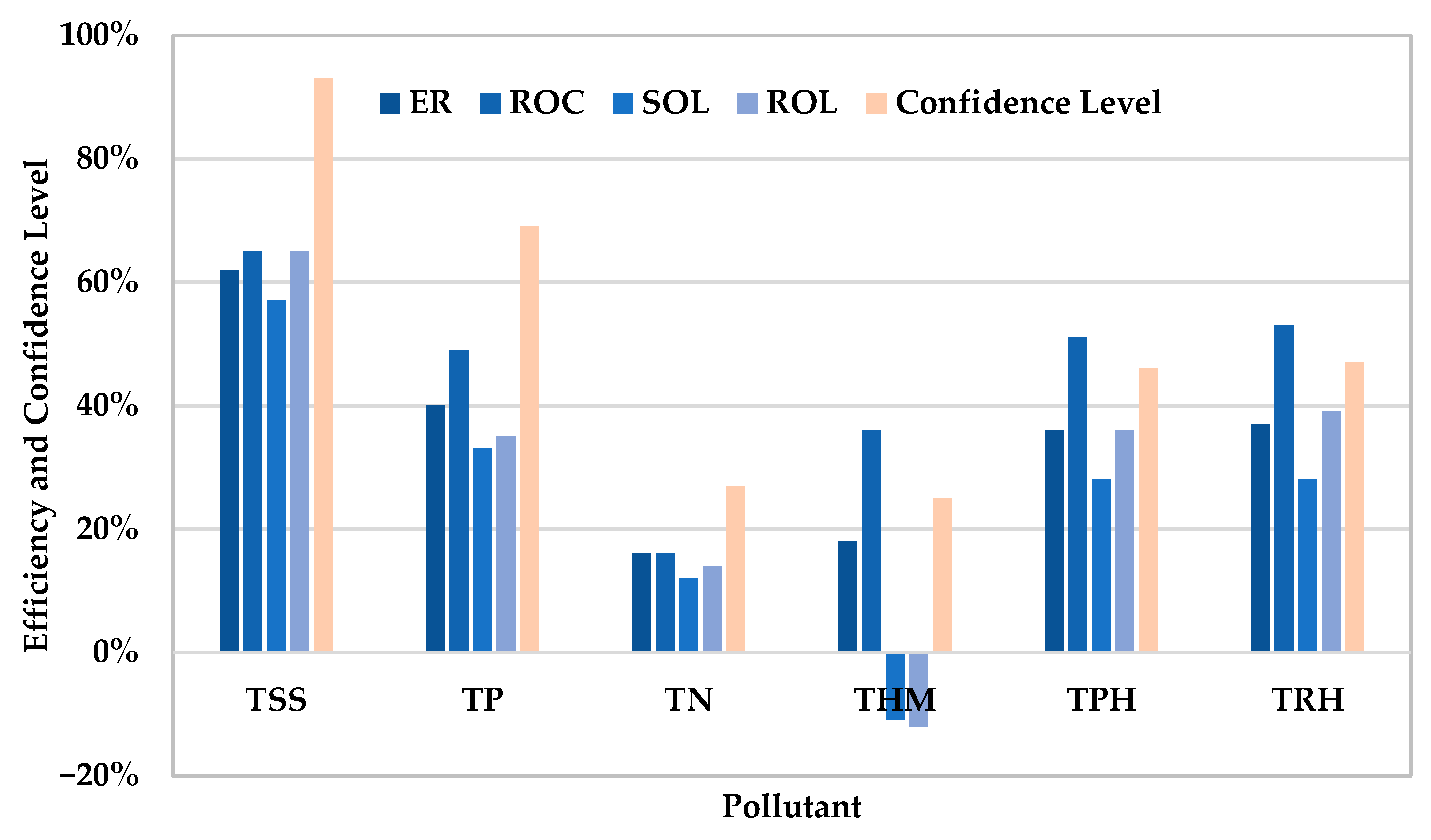
Based on the formulas presented in Table 1, the ER and SOL for all qualifying events and for each pollutant calculated are shown in

Table 8. Efficiency results for Ecosol Litter Basket.

Pollutant	Concentration Efficiencies		Load Efficiencies		Confidence Level (EMCin, EMCout)
	ER 1	ROC	SOL	ROL
TSS	62%	65%	57%	65%	93%
TP	40%	49%	33%	35%	69%
TN 2	16%	16%	12%	14%	27%
THM 2	18%	36%	−11%	−12%	25%
TPH	36%	51%	28%	36%	46%
TRH	37%	53%	28%	39%	47%

¹ Calculated based on simple mean value. ² the efficiency results for TN and THM are not statistically significant.

and Figure 11. It is noted that the highest values of ER and SOL were achieved for TSS (62% for ER and 57% for SOL), whereas the lowest values of ER and SOL were achieved for TN (16% for ER and 12% for SOL) and THM (18% for ER and −11% for SOL). From the results, as highlighted in Figure 11, it is observed that there is a consistent agreement between the results of concentration and load efficiencies for TSS, TP, TN, TPH, and TRH. It is also observed that the required confidence level of 90% [1] was only achieved for the pollutant type TSS. It is important to note that the results for TN and THM are included for completeness, as evaluated in Section 3.1 the differences between the EMCs for the influent and effluent streams for TN and THM were not found to be statistically significant.

By way of comparison, in [11] field testing results for a stormwater device consisting of a similar treatment train with a 200-micron mesh pit basket were presented. The site was predominantly roof area (56% coverage). Based on an analysis of nine qualifying events, the reported efficiency ratios were 32% for TSS, 37% for TP, and 38% for TN for the pit basket. Reference [10] completed a combined laboratory and field test study of the Ecosol Litter Basket. The mean value of collection efficiencies was evaluated to be 29% for TSS, 40% for TP, 11% for TN, 6% for THM, and 20% for hydrocarbons [10]. In [12], field testing of a gross pollutant trap (GPT) was undertaken over a period of two years at a commercial site located in Queensland, Australia. Approximately 85% of the total catchment area was impervious. The efficiency ratio (ER) calculated for the GPT was found to be 49% for TSS, 27% for TN, and 41% for TP.

4. Conclusions

Within this paper, the results from a field-based performance analysis of the Ecosol Litter Basket are presented, where the results are based on the analysis of over 29 rainfall events, collected over a two-year period, within an urban catchment in Australia. Between 13 to 16 events were evaluated as qualifying for the purposes of characterizing the removal efficiency [1].

A variety of pollutant removal calculation methods, including concentration and load metrics, were utilized in this study to evaluate the efficacy of the performance of the device. In regard to the regression of loads (ROL), since a nonlinear regression is often more suitable for influent and effluent load data, a new approach presented by [18] was used for this metric. Regression of concentrations (ROC), as a new concentration-based metric introduced in [18], was also used to facilitate characterization of removal efficiency. It is strongly suggested that both concentration-based metrics (ER and ROC) and load-based metrics (SOL and ROL) be calculated for characterizing the performance of a stormwater filtration device.

The statistical significance analysis showed the difference in event mean concentrations for the influent and effluent streams to be statistically significant for TSS, TP, TPH, and TRH. For the range of metrics considered, the statistically significant removal efficiencies of the Ecosol Litter Basket are summarized as: between 57–65% for TSS with the influent EMC up to 142 mg/L; 33–49% for TP with the influent EMC up to 0.32 mg/L; 28–51% for TPH with the influent EMC up to 3.82 mg/L; and 28–53% for TRH with the influent EMC up to 3.95 mg/L. Given the high variability observed in the EMC data, only the TSS results are estimated with high confidence.

References

- Storm Water Australia. Stormwater Quality Improvement Device Evaluation Protocol (SQIDEP); Stormwater Australia: Brisbane, Australia, 2018. [Google Scholar]
- The University of Adelaide (UoA). Ecosol Litter Basket Field Study Report A: Bench Top Study on Matching the Field Site and Treatment Device; A157123-A-S3; The University of Adelaide (UoA): Adelaide, Australia, 2016. [Google Scholar]
- Turco, M.; Brunetti, G.; Carbone, M.; Piro, P. Modelling the hydraulic behaviour of permeable pavements through a reservoir element model. In Proceedings of the 18th International Multidisciplinary Scientific GeoConference SGEM 2018, Albena, Bulgaria, 2–8 July 2018. [Google Scholar] [CrossRef]
- Turco, M.; Brunetti, G.; Palermo, S.; Capano, G.; Grossi, G.; Maiolo, M.; Piro, P. On the environmental benefits of a permeable pavement: Metals potential removal efficiency and Life Cycle Assessment. Urban Water J. 2020. [Google Scholar] [CrossRef]
- Brunetti, G.; Turco, M.; Carbone, M.; Maiolo, M.; Piro, P. Modelling the hydraulic behaviour of green roofs through a semi-conceptual reservoir element model. Proceedings of 18th International Multidisciplinary Scientific GeoConference SGEM, Albena, Bulgaria, 2–8 July 2018. [Google Scholar]
- Carbone, M.; Turco, M.; Nigro, G.; Piro, P. Modelling of hydraulic behaviour of green roof in catchment scale. Proceedings of International Multidisciplinary Scientific GeoConferences SGEM 2014, Albena, Bulgaria, 17–26 June 2014; pp. 471–478. [Google Scholar] [CrossRef]
- Zhong, R.; Xu, M.; Netto, R.; Wille, K. Influence of pore tortuosity on hydraulic conductivity of pervious concrete: Characterization and modelling. Constr. Build. Mater. 2016, 125, 1158–1168. [Google Scholar] [CrossRef]
- University of South Australia. Evaluation of RSF100 and RSF2000 Gross Pollution Traps; Urban Water Resources Centre Report: Adelaide, Australia, 1996. [Google Scholar]
- University of South Australia. Evaluation of RSF100 Gross Pollution Trap—Stage 2; Urban Water Resources Centre Report: Adelaide, Australia, 1996. [Google Scholar]
- The University of Adelaide. Performance Review of the Ecosol Litter Basket at-Source Solid Pollutant Filter; The University of Adelaide (UoA): Adelaide, Australia, 2013. [Google Scholar]
- Drapper, D.; Hornbuckle, A. Field Evaluation of a Stormwater Treatment Train with Pit Baskets and Filter Media Cartridges in Southeast Queensland. Water 2015, 7, 4496–4510. [Google Scholar] [CrossRef] [Green Version]
- Nicholas, P.; Lucke, T. Field Evaluation of the Nutrient Removal Performance of a Gross Pollutant Trap (GPT) in Australia. Sustainability 2016, 8, 669. [Google Scholar] [CrossRef] [Green Version]
- Nichols, P.; Lucke, T.; Drapper, D. Field and Evaluation Methods Used to Test the Performance of a Stormceptor® Class 1 Stormwater Treatment Device in Australia. Sustainability 2015, 7, 16311–16323. [Google Scholar] [CrossRef] [Green Version]
- Stanford, R.; Yu, S. Field Evaluation of a Stormwater Bioretention Filtration System. In Proceedings of the World Environmental and Water Resources Congress, Tampa, FL, USA, 15–19 May 2007. [Google Scholar]
- Shammaa, Y.; Zhu, D.Z. Techniques for Controlling Total Suspended Solids in Stormwater Runoff. Can. Water Resour. J. 2001, 26, 359–375. [Google Scholar] [CrossRef]
- National Institute of Water & Atmospheric Research Ltd (NIWA) Consultant for Environment Southland. Design of Stormwater Monitoring Programs; Environment Southland: Auckland, New Zealand, 2014. [Google Scholar]
- Urban Asset Solutions (UAS). Drawing RSJ0148-A008, Site 7—RCC Depot—Litter Basket Catchment Summary; UAS: Adelaide, Australia, 2015. [Google Scholar]
- Pooya Nejad, F.; Zecchin, A.C. Stormwater Filtration Performance for the Ecosol Storm Pit (Class 2): Statistical Analysis of Field Data. Water 2020, 12, 2723. [Google Scholar] [CrossRef]
Figure 1.
Catchment plan. Adapted with permission from ref. [17]. Copyright 2015 Urban Asset Solutions (UAS). (Image @2021 Google Maps).
Figure 2.
Installed Ecosol Litter Basket: (a) Device schematic, (b) top-down view of device, (c) device as installed.
Figure 3.
Installed instrumentation: (a) Instrumentation layout; (b) Equipment cabinet; (c) Rain gauge; (d) data loggers; (e–g) Autosampler.
Figure 4.
Flow sensor and sample intake locations. Reprinted with permission from ref. [17]. Copyright 2015 Urban Asset Solutions (UAS).
Figure 5.
Bar plots for event mean concentration for all pollutants.
Figure 6.
Box and Whisker plots for event mean concentration for all pollutants.
Figure 7.
Cumulative probability plots for all pollutants.
Figure 8.
Regression of loads (ROL).
Figure 9.
Regression of concentrations (ROC).