
Numerical Analysis of Enhanced Conductive Deep Borehole Heat Exchangers


1
Energy and Power, Cranfield University, Cranfield MK43 0AL, UK
2
Earth Sciences Division 90-1116, Lawrence Berkeley National Laboratory, Berkeley, CA 95720, USA
3
James Watt School of Engineering, University of Glasgow, Glasgow G13 8QQ, UK
*
Author to whom correspondence should be addressed.
Sustainability 2021, 13(12), 6918; https://0-doi-org.brum.beds.ac.uk/10.3390/su13126918
Submission received: 12 May 2021
/
Revised: 11 June 2021
/
Accepted: 13 June 2021
/
Published: 19 June 2021
(This article belongs to the Special Issue Numerical Simulations and Optimization of Renewable Energy Systems)
Abstract
:Geothermal energy is a reliable and mature energy source, but it represents less than 1% of the total renewable energy mix. While the enhanced geothermal system (EGS) concept faces technical validation challenges and suffers from public acceptance issues, the development of unconventional deep-well designs can help to improve their efficiency and reliability. Modelling single-EGS-well designs is key to assessing their long-term thermal performances, particularly in unconventional geological settings. Numerical results obtained with the T2WELL/EOS1 code have been validated with available experimental data from a deep borehole heat exchanger (DBHE), where a temperature of 358 C has been measured at a depth of 1962 m. Based on a calibrated model, the thermal performances of two enhanced thermal conductive DBHEs with graphite were compared for high geothermal gradients. The analysis highlights the potential recovery of a variable fraction of vapour. Graphite used along the well appears to be the most suitable solution to enhance the thermal output by 5 to 8% when compared to conventional wells. The theoretical implementation of such well in the Newberry volcano field was investigated with a single and doublet DBHE. The findings provide a robust methodology to assess alternative engineering solutions to current geothermal practices.
1. Introduction
The geothermal energy sector has proven its ability to provide base load electricity and heat, but still requires further advancements to overcome the technical and site specific limitations. Enhanced geothermal systems (EGS) have been shown to theoretically access geothermal energy widely, and to produce electricity at lower costs and with fewer geographical constraints [1]. A hydraulic stimulation is usually needed to ensure the creation of a connected path-flow in artificial fractures. This process has been successfully achieved in several field sites [2]. A large volume of water injected at low pressure has been notably efficient at generating enhanced fracture permeabilities in the Newberry Volcano EGS demonstration site [3]. However, the commercialisation of EGS has not yet been validated due to induced seismicity issues [4], poor reservoir connectivity, and the absence of long-term regulatory policies in place [5].
EGS single-well methods can provide an alternative solution to make stimulation unnecessary, by circulating a working fluid in a sealed well, or by connecting the wellbore to pre-existing fractures or in-situ geothermal fluids [6,7,8,9]. Closed wellbores such as borehole heat exchangers have been conventionally investigated for depths less than 1000 m [10,11]. To date, deep borehole/coaxial heat exchangers (DBHE/DCHE) have mainly been used for heating and cooling purposes [12,13]; they have also been proposed as a heat extraction method above magma bodies to exploit unattractive low productive geothermal zones (typically non-permeable) [14]. The DBHE performances have been shown unaltered by the recovery cycles with identical flow rates in the Weggis plant, Switzerland [13]. For this type of system, the working fluid (water, CO2 or isobutene) only circulates in a closed well through an annular space [6] or through different systems such as U-tubes or parallel DBHEs [15,16], without geothermal fluid production. Various technology-derived concepts, such as horizontal BHEs, can provide long-term heat power in the range 0.35–2.0 MW. For such systems, three different decreasing temperature slopes as functions of the horizontal section length have been studied [8,17]. A U-shaped well filled with CO with a flow rate of 25 kg/s has been shown to provide more than 2.5 MW, with a thermosiphon [18], without pumping.
Closed-wellbore models are generally coupled with a reservoir model to account for the heat exchange and fluid flow in the surrounding porous or fractured rocks [6]. Fast simulations using a finite line source model have also been performed to investigate intermittent conditions in a DBHE [19]. Closed wells have been investigated with several geothermal gradients from 25 to 50 C/km and between 2 to 6 km. When considering 50 C/km, the power production starts to be economically viable at depths more than 3 km. In addition, direct power generation systems have appeared more efficient with supercritical fluids than flashing power generation systems [20]. The application of DBHEs worldwide reaches a maximum depth of 3 km when generating 0.15 to 2.5 MW of thermal power and 0.25 to 364 kW of electrical power [6]. In deep reservoirs, the DBHE’s installed capacity has been shown to be highly sensitive to the reservoir’s porosity and the rock’s thermal conductivity [21]. The well’s thermal conductivity is a function of the material used (e.g., one layered with steel or double layered with a vacuum), with values down to 10 W/m·K for the inner pipe in [22]. The thermal insulation of the inner pipe, the mass flow rate and the geothermal heat flux are the most important parameters affecting the thermal performances.
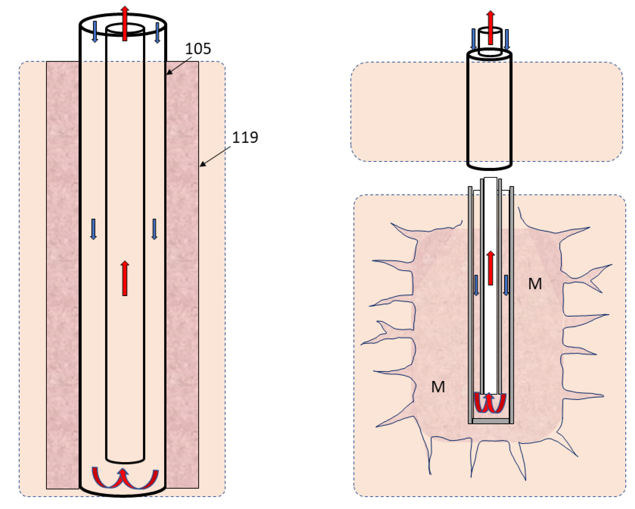
Various numerical and analytical tools have been used to investigate DBHEs [6]. The use of the constant fluid properties assumption generates errors in the calculation of the thermal and pressure losses in the DBHE [23]. While the assumption of constant water properties can be acceptable in a low geothermal gradient context (1.8% difference in the thermal resistance in [24] for 30 C/km), this is no longer valid in high geothermal gradients and for deeper DBHEs. Assuming constant water properties can underestimate the temperature of the water produced and heat flux for a DBHE of 6100 m [25] and can overestimate the performances by 11% in a DBHE of 3500 m [26]. Therefore, the use of pressure-temperature dependent thermophysical properties is important, especially the fluid specific heat, the viscosity and the thermal conductivity [27]. The overall performance of a DBHE is limited by the surface heat exchange (in the wellbore) between the working fluid and the reservoir, which renders those systems more efficient for supplying heat rather than electricity, even in the case of very high geothermal gradients [28]. To increase the thermal performances of DBHEs, different patented well designs could increase the heat transfer rate of DBHEs/DCHEs by enhancing the well thermal properties. Figure 1 (Left) shows the implementation of graphite between the external casing and the rock around a single well, proposed by Hara [29], using highly conductive fillers of graphite between the external casing (105) and the cement or surrounding rocks (119) of a DCHE.
As the cement thermal conductivity is a key parameter [31], the injection of highly conductive materials such as graphite (500 to 140 W/m·K) into the well surroundings has been proposed by Buchi [30] to create an enhanced conductive area with the injection of a high conductive material M in the near bottom hole (see Figure 1 Right). Despite requiring injection processes in Buchi’s technology, these innovations would empower DBHEs under certain conditions, as numerically evaluated in [32]. If the heat transfer rate is sufficient, both technologies described in Figure 1 could produce a variable vapour fraction. The additional use of a downhole choke, or a boiler, could facilitate the phase change process by decreasing the pressure, as proposed in [7].
After presenting and validating the DBHE numerical model, this study investigates the heat recovery of enhanced DBHE/DCHEs designs for different theoretical geothermal settings, using the T2Well integrated wellbore–reservoir simulator [33], considering graphite in the well surroundings. At last, a numerical case study in the Newberry EGS system is presented.
2. Materials and Methods
This section introduces the experimental DBHE used to validate the numerical model, followed by the mathematical formulation of T2Well and the settings of the DBHE numerical model. The geometries considered for the investigation of the two theoretical DBHE patents with graphite in different geothermal environments are presented, and compared with a conventional DBHE, without graphite. The parameters used in a 2D numerical DBHE doublet model are described. These parameters are used to investigate the DBHE performances in an EGS case study.
2.1. Model Description
Figure 2 (Left) shows a DCHE-DBHE used in the HGP-A well in Hawaii [34], in basaltic formations, with the downward injection of water through an external annulus. The grey filled material between the casing sections is the cement. Figure 2 (Right) shows a view of the orthogonal mesh generated, highlighting the wellbore flow domain and the rock domain extended to the radial distance of 100 m. As the water flows down, it is heated before flowing back to the surface and requires pumping or is self-rising due to the thermosiphon effect via the internal tubing.
As the system is fully sealed, no contact between the geothermal fluids (or rocks) and the water takes place. In addition, the cement surrounding the well has been replaced by a highly thermally conductive material, graphite in the present study, to investigate the potential of both patents.
2.2. Mathematical Formulation
T2Well/EOS1 is a wellbore reservoir simulator with a 1D, two-phase momentum equation for the wellbore and the 3D multiphase Darcy law in the reservoir [33]. T2Well solves the mass and energy balance equations numerically using a finite difference scheme. The momentum balance equation for the wellbore flow is solved numerically with a semi-explicit scheme [35]. The code has been applied previously to model closed-loop U-shaped geothermal wells [18], and other cases [33]. It uses the IAPWS-IF97 formulation for water [36]. The connections between the well and the formations have been closed to fluid flow so that only the conductive heat transfer between the wellbore and the surrounding formations is considered. Kinetic energy is considered in the wellbore where velocity can be high and is ignored in the reservoir at low fluid velocities. The conservation of mass for a two-phase system is written as [33]:
The conservation of energy in the reservoir and wellbore are:
The liquid and gas velocities in the geothermal formations are calculated as:
where k is the absolute permeability; is the phase relative permeability; are the sums of the respective phase pressure (gas) and the capillary pressure in the porous media. The parameters and their units are described in the Nomenclature.
A drift flux model (DFM) is used to model the interfacial interactions between the gas and the liquid, assuming that the gas velocity is related to the volumetric flux of the mixture. The DFM treats the drift velocity as an average, efficiently solving the complex two-phase flow in the wellbore [35]. The drift velocity of gas and the momentum equations of a two-phase flow in the wellbore are presented in Appendix A. The Equation of State 1 (EOS1) module has been used with T2Well in this work [37].
2.3. Model Validation
To apply T2Well in high-temperature settings with various vertical closed loop designs, the experimental data from the HGP-A well in Hawaii have been used to model a DBHE in a volcanic geothermal system. A temperature of 358 C was measured at a depth of 1962 m. After having sealed the well, the experiment was performed in a 7” casing by installing an insulated internal tubing up to the depth of 876.5 m, i.e., 3 m above the bottom of the test section. A water mass flow rate of 1.33 kg/s at 30 C was injected into the annular space for 7 days. A maximum thermal output powers of 373 kW, and 76 kW were measured after 7 days [34]. The experiments aimed to validate a heat extraction method in low-production geothermal reservoirs, and super-hot rocks adjacent to solidified magma bodies [14].
An axisymmetric mesh refined near the well to consider the casing and cement sections shown in Figure 2 (Right) has been used with the numerical code T2Well/EOS1. The top of the reservoir was assumed to be 30 C and 1 bar; a temperature of 350 C was set as a constant at 1931 m, as described in [14]. Table 1 shows the different casing and cement properties of the experimental settings considered in the numerical model. The T2Well-based simulation, experimental data and pressure–temperature simulations from [34] were all based on the thermal parameters listed in Table 1. The mesh contained 1310 cells, starting with a radial cell distance corresponding to the well geometry shown in Figure 2 (Left), and increasing the lateral cell sizes following a logarithmic discretisation up to the radial distance of 100 m. The formation, casing and cement were considered with no porosity nor permeability. The roughness height of the well, including bottom edge, was varied between 25 and 85 m.
Without information on the well roughness in [34], the model was compared against the experimental data by varying the roughness values of the well walls (25–85 µm) and the user-specified perimeter of the bottom Section (10–12 m), generating pressure losses due to the DBHE geometry. After validating the DCHE numerical model with the experimental data from [34], a DCHE T2Well/EOS1 simple model without the centralizers was applied to investigate different high-temperature geothermal environments.
2.4. Theoretical Analysis of Enhanced DCHEs
A DBHE using graphite with a thermal conductivity of 300 W/m·K and a heat capacity of 710 J/kg·K was considered in [32]. The use of graphite instead of cement around the casing for the Hara patent (Figure 1 Left, between casing 7” and 9 5/8”) and in the surrounding formations according to the Buchi patent was assumed to be only conductive. Figure 3 presents the vertical and radial directions used for the analysis of both patents. The implementation of graphite vertically along the wellbore, as proposed in [29] has been varied from 50 to 200 m from the bottom depth of the DBHE and then for the whole length (All Hara). The influence of the horizontal extension of the enhanced conductive chamber described in the Buchi patent has been investigated for radii (r) of 50 cm, 1 m and 5 m with a constant vertical length of 30 m from the bottom of the DBHE. Its vertical extension has been varied from 30 to 100 m with a constant radial distance (r) of 50 cm.
The top of the theoretical reservoir models were set at 1 bar and 10 C, with a homogeneous rock porosity of 10 % and a permeability of 10m. The thermal properties of rocks are described in Table 1. The two patents have been compared for case 1 against the base case without graphite implementation. The most efficient and cost effective solution has been identified and tested for the remaining cases 2–5 described in Table 2.
2.5. Case Study: Implementation of a DBHE in an EGS System
The Newberry Volcano site hosts a demonstration EGS to investigate low pressure stimulations and microseismicity monitoring [3]. To obviate the stimulation process and still access the heat, a DCHE has been considered instead of the well NWG 55-29 in Newberry, using the well materials described in Section 2.3. The wellbore is based on the NWG 55-29 well schematic from [3] with the tubing diameter of 3 1/2” from [14], and a vertical gap of 3 m between the bottom of the tubing and the bottom of the well (3067 m). It uses the initial temperature log in the well NWG 55-29, shown in Figure 4, with 12 C at the surface.
The mesh was adapted with the formations shown in Table 3, taken from a previous TOUGH2-based study [38]; the density of the formations is 2700 kg/m. The thermal influence of graphite on the wellbore has been studied and compared to a DCHE with a conventional material casing, as investigated in [39].
A 2D DBHE doublet model has been built to investigate the potential increase of the thermal performances due to production and loading cycles. Two identical DBHEs located 50 m apart in the Newberry volcano environment have been modelled. The 50 m distance was assumed to be sufficient to avoid a thermal breakthrough between the DBHEs considering the time of simulation (240 h).
Alternating imposed injections are considered in each DBHE for different periods: 6, 24 and 168 h. For the first period, water circulates at 5 kg/s in a DBHE (DBHE1), and the second DBHE (DBHE2) has no mass flow rate imposed (loading phase). In the following period, 5 kg/s is applied to DBHE2 while DBHE1 is under a loading phase.
3. Results
The comparison between the results from the numerical validation model and the experimental DBHE is presented, highlighting the model’s sensitivity to match the return pressure. The return water temperature and potential energy production and benefits of using DBHE patents with graphite are analysed with a DBHE base-case, without graphite. This study is completed with the analysis of a single DBHE and a DBHE doublet with graphite in the Newberry EGS case study.
3.1. T2Well DCHE Model
3.1.1. Parameter Analysis
Figure 5 shows the simulated return pressures at the surface of the tubing compared with the experimental data from [14]. When the perimeter was decreased (12 to 10 m), an increase of the surface pressure was observed.
For an increase of the wall roughness from 25 to 85 µm, the simulated surface pressure decreased, still without capturing the early drop of pressure. The measured decrease of pressure at 1 h approximately matched when the roughness height of the annulus and tubing were assumed to be different, 25 µm for the annulus and 85 µm for the tubing. This might correspond to the difference of roughness of the wells between the novel tubing (vacuum type double tube insulated pipe) and the old casing in the annulus of the well HGP-A [14].
As can be seen in Figure 5 for t < 2 h, two early waves of pressure were present, potentially due to the presence of cement and sand particles in the experiments [14]. The first peak could also have been a result of the cold (high density) water residing in the upper portion of the tubing, being substituted by the hot (lower density) water flowing from deeper zones, reducing the pressure drop in the tubing, resulting in higher wellhead pressure. The outlet pressure increase was not sustainable because the amount of hot water was limited in volume. The second peak reflects the arrival of water from the annulus, which was due to the injection of cold water which replaces warm water from the initial stage. The time period between these two peaks depends on the system parameters being applied, which can make them merge into a single peak, or make them separate further. The resistance to flow at the bottom of the tubing has been found to be the most sensitive parameter to control the return pressure simulated. As shown in Figure 6, the temperature was not significantly affected by the parameter changes, and was mainly constrained by the formations and well thermal properties.
3.1.2. Model Validation
The final model has been obtained using a well roughness height of 55 µm, which corresponds to the roughness of steel pipes [40], and applying the parameters presented in Section 2.3. The numerical results of long-term pressure over time show a good match with experimental data and simulations from [34]; see Figure 7. The temperature profile after 93 h in both the annulus and the tubing has also been compared with the measurements from [34]; see Figure 8. A difference of 1.8 C and a difference of 1.7 C were obtained at the bottom and top of the DBHE, respectively, compared to the measurements. Numerical results obtained with T2Well are in satisfying agreement with both experimental data and numerical results from [34].
Note that the cement has been modelled without saturated water, which is different from [34]. This might have induced a small temperature difference. Furthermore, without explicit definition of the DBHE bottom, the 1D-based return flow calculation shows difficulties in accurately matching the experimental results. Despite uncertainties in reproducing the early drop of pressure but with acceptable long-term simulation results, the T2Well DCHE/DBHE model has been used for further studies in the following sections.
3.2. DBHE Patent Analysis
3.2.1. Thermal Performance Comparison
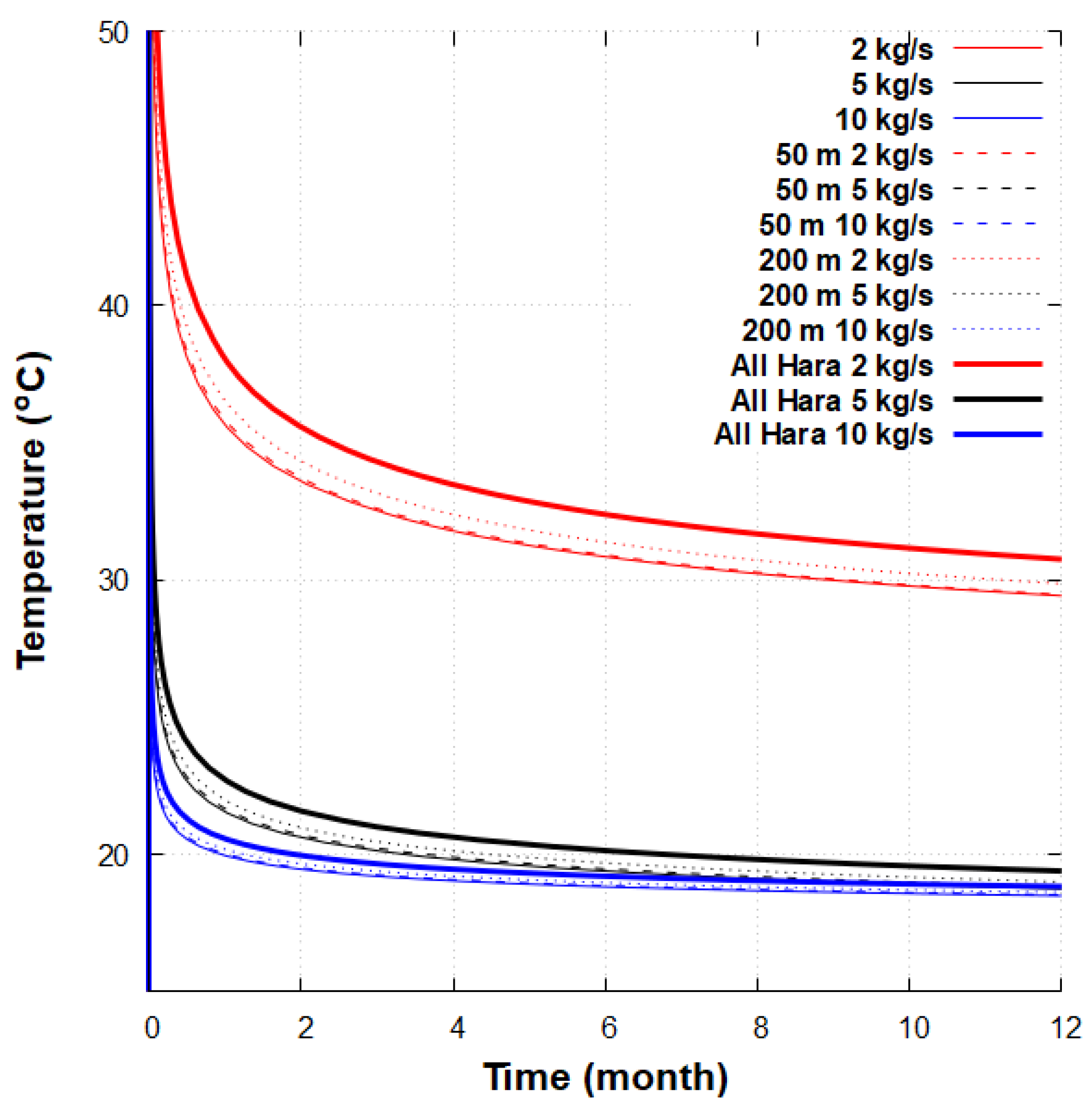
A comparison between the two patents has been performed with case 1, using a DBHE length of 1000 m and a geothermal gradient of 170 C/km. The wellhead temperature of a DBHE using graphite along the wellbore in the vertical direction (c.f. Figure 3) is presented in Figure 9 and compared to the base case without graphite. As described in [28,31], the mass flow rate is a major constraint on the water temperature recovery as the resident time of water in the DBHE was shorter for a high mass flow rate.
The long-term wellhead temperature showed an early increase (rising from 10 C to more than 50 C), before exhibiting a transitional behaviour, and a slow decrease after 2 months. The high thermal conductivity of graphite provided a higher water temperature recovery, and higher if the mass flow rate in the DBHE was slower. Increasing the vertical length of graphite along the well enhanced the DBHE heat transfer.
Similarly, the use of graphite in the surrounding formation, which provided an enhanced conductive chamber around the DBHE, increased the heat recovery compared to the base case (Figure 10). The extension of graphite at the bottom of the DBHE, 5 m in the horizontal direction and 100 m in the vertical direction, induced an increase of the temperature. After 1 year, the bottom temperature decreased by 8 to 10 m around the well. The heat extraction was higher with a higher mass flow rate and implied a lower local temperature distribution.
The geometric calculation in Table 4 suggests that Hara’s patent needs less high conductive material compared to Buchi’s patent. The formation parameters, such as the thermal conductivity, permeability, porosity and the effect of applying a double porosity model [41] in a graphite fractured network, have not been considered here. In areas with a geothermal gradient ranging from 20 to 40 C/km, the presence of thick subsurface aquifers with high in-situ velocities can enhance the forced heat convection [31]. Assuming the technical feasibility of injecting highly conductive fluids into the wellbore surroundings, this study in a low permeable geothermal context shows that the thermal properties of the well are more advisable for investigation to improve the overall DBHE economics rather than artificial improvements of the surrounding rock’s thermal properties.
Due to the expensive technical operations and graphite injection volume required in Buchi’s patent, the following sections discuss the energy assessment using only the graphite injection along the wellbore length, as proposed by Hara [29].
3.2.2. Energy Production
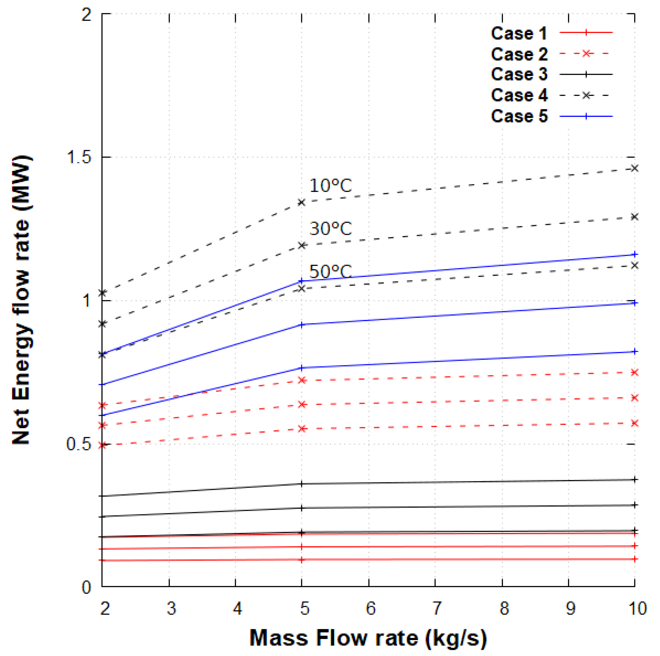
The net energy flow rate produced after 1 year from a DBHE with graphite is presented in Figure 11, varying the length of the DBHE, the geothermal gradient, the mass flow rate and the injection temperature. The values are detailed in Table 5, which shows the net energy gain by the difference of the produced and injected energy flow rates. The depth of the DBHE appears to guarantee a higher energy recovery, according to the value of the geothermal gradient. Indeed, the surface heat exchange and residence time are maximised. In Figure 11, the increase of mass flow rate in the DBHE enhances the energy flow rate for all cases. The net gain in case 4 at 10 kg/s reaches 1.45 MW after 1 year. Inversely, the injection of hot water decreases the net energy flow rate.
The total net energy flow rate after 1 year exceeds 1 MW for a DBHE of 3990 m (cases 4 and 5) for a low injection temperature and mass flow rates higher than 5 kg/s. Table 5 provides the percentage of increase calculated as the difference of energy flow rate produced and injected in the DBHE compared to the DBHE base case. The values show an increase of the long-term performances between 5.4 and 8.4%. Numerical results show that the efficiency increase using graphite is higher for high mass flow rates and high injection temperature. At low mass flow rates, the benefit of using high conductive material decreases for the deepest DBHEs. Despite limiting risks such as induced seismicity, the net energy gain values from a graphite filled DBHE are limited compared to the potential from an operating EGS for producing electricity, by up to several MWe per well [2].
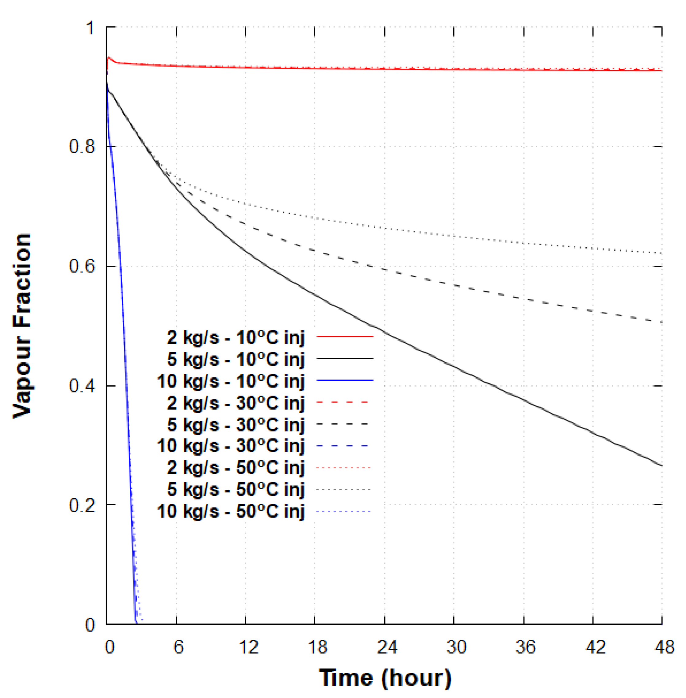
Figure 12 shows the fraction of vapour produced, for example, in case 4, with potentially a very high energy output for the first 48 h. A high injection temperature extends the vapour fraction existence for a mass flow rate of 5 kg/s. This fraction could be used to drive vapour after separation to a turbine and generate power. As an example, in the first 6 h of production, the energy gain reaches over 3 MW for a flow rate of 2 to 5 kg/s.
3.3. Newberry Case Study
3.3.1. Analysis of a DBHE with Graphite
The temperature in the annulus and inner pipe of a DBHE implemented with and without graphite along the wellbore in the Newberry Volcano site is shown in Figure 13 after 1 year, and a water injection temperature of 10 C. With a low flow rate, the vertical temperature in the well is high, with higher heat losses when the water rises to the surface. When using graphite, the energy flow rate after 1 year improves by 5 to 7%, reaching 1.05 MW at 2 kg/s, 1.51 MW at 5 kg/s and 2.19 MW at 10 kg/s.
However, higher friction pressure losses require pumping if the flow rate is high. The pressure difference between the injection pressure and the outlet surface pressure is shown in Figure 14. If the value is negative, no pump is needed, highlighting a thermosiphon effect. Thus, the system can operate at low flow rates, around 2 kg/s, without pumping.
As mentioned previously, the total flow rate and energy recovered using this type of single enhanced DBHE is very low compared to the economical expectations from a matured EGS (80 kg/s for several MW of power generated), but it offers a reliable and an easily monitored source of energy. If a DBHE field were to be planned, a full economic analysis balancing the lower risks of the closed-loop systems with the higher risks of EGS could be performed using modelling tools. Additionally, closed-loop wells offer the potential to retrofit poorly productive geothermal or oil and gas fields by implementing DBHEs in abandoned wells [42,43].
3.3.2. Alternating Heat Recovery with a DBHE Doublet
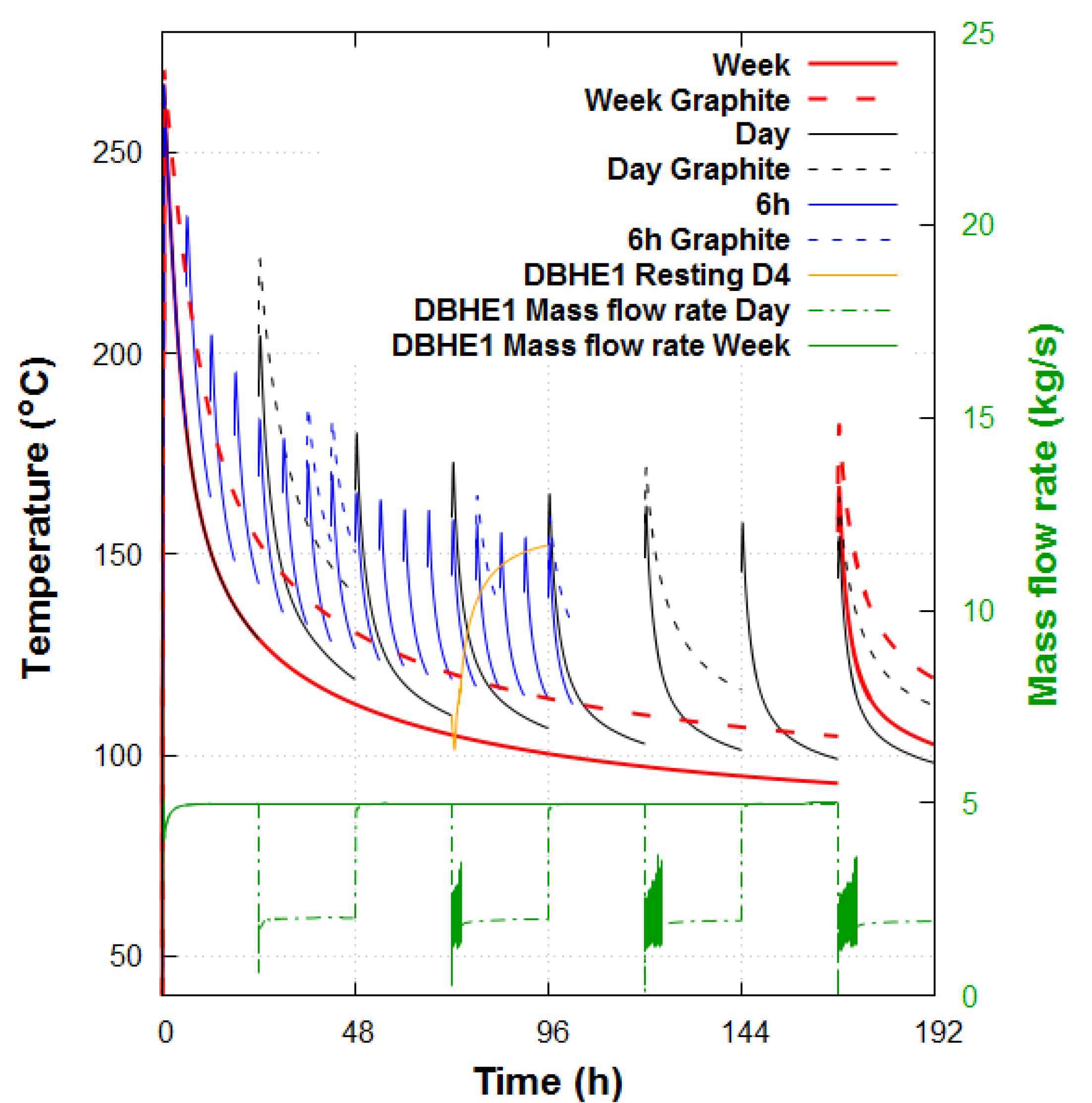
Figure 15 shows the alternate temperature at the surface from the production DBHE only with a flow rate of 5 kg/s, for the three periods with and without graphite on the wellbore.
Similarly to the previous observations, the graphite enhances the heat recovery for all the cases. While one week of continuous production provides the lowest wellhead temperature, alternating injections of 6 or 24 h cycles ensure higher temperatures and less thermal variability. Shortening the injection/production cycles slows down the temperature drop with lower peaks, as observed for a single well’s production.
The mass flow rate through one DBHE with a daily or weekly injection cycle is shown at the bottom of Figure 15. When the injection is stopped at 24 h, oscillations appear before reaching a residual flow rate (around 2 kg/s). This is due to the hotter and lighter water at the bottom being driven upwards in the tubing to the surface, replacing the cold and denser water. The temperature at the surface of the resting well on the fourth day (DBHE Resting D4) shows the thermal loading of the latter, before starting another cycle. Despite highly variable wellhead temperatures, short cycles can increase the overall thermal performances with a doublet DBHE compared to a long-term steady production.
In the case with graphite for 6 h cycles, a total flow rate of 7 kg/s from both wells provides 4.14 MW at 96 h (2.88 MW at 5 kg/s and 1.26 MW at 2 kg/s). For a 24 h cycle (2.66 MW at 5 kg/s and 1.42 MW at 2 kg/s) and weekly cycles (2.46 MW at 5 kg/s and 1.62 MW at 2 kg/s), it reaches 4.08 MW at 96 h. For daily and longer cycles, an approximate constant total of 4 MW from both DBHE is reached as the resting well delivers more energy at 2 kg/s for an equivalent longer resting period. For 6 h cycles, an additional 60 kW is calculated at 96 h, highlighting the benefit using shorter cycles, which sustain higher heat recovery. The selection, from an operator point of view, can also be driven by the energy variability using shorter or longer cycles.
4. Discussion
Our numerical assessment of highly conductive materials in DBHEs and innovative closed-loop well patents provides insights into their potential performances in various settings. In this work, the influence of alternating injection and resting periods for a DBHE with high-temperature gradient settings is shown to be non-negligible compared to DBHEs being a mean geothermal gradient such as in Weggis, Switzerland [13]. The increase of the DBHE length in Newberry (3067 m) compared to the DBHE in Weggis (2295 m) can also explain this difference, due to the increase of the surface heat exchange. Further research on very short cycles can be pursued to target only the high-temperature peak and investigate whether the recovery period in high geothermal gradients is long enough to supply a sustainable amount of energy. The unconventional implementation of enhanced DBHEs [32] needs further investigation close to a magmatic object with realistic heterogeneous geological formations, as in the IDDP-1 project [44,45], or in deeper zones, in crustal bodies [46], to overcome the current technical limitations.
T2Well/EOS1 is a 1D wellbore simulator, which might encounter challenges when modeling real 3D flows in unconventional well geometries, such as the bottom of a DBHE. Despite the model validation obtained from an experimental study, the numerical model might provide inaccurate results for deeper DBHEs with other specific geological conditions and without experimental data. Multiphysics codes [26,28] can target the complex geometry in specific well sections to strengthen the heat performance analysis and the pressure loss assessments. Supercritical CO and organic fluids can also be used to extract the heat from low permeable and high-temperature geothermal systems to counterbalance the high pressure losses using pure water, but with a high energy extraction rate [18,20]. As super hot EGS are targeted at accessing high temperatures—up to 450 C in Newberry [47], 500 C for the DESCRAMBLE project in Italy [48] and the Magma Test Bed in Iceland [49], higher temperature capabilities need to be implemented in the current numerical modelling software and tools to investigate the wellbore-reservoir interactions.
5. Conclusions
The modelling of enhanced conductive DBHEs on a high geothermal gradient has been conducted. A coupled wellbore/reservoir, two-phase flow simulator, T2Well, has been used to simulate the heat transfer processes. The thermal performances of the two patents enhancing the conductive DBHE/DCBHEs in a formation in high geothermal gradients have been compared for one year. The effects of the geothermal gradient, depth, mass flow and temperature injection were analysed, and the following conclusions can be drawn:
- T2Well can be used to investigate DBHEs, showing a good agreement with experimental data. The user-specific perimeter of the bottomhole and the well roughness play a major role in the pressure response of the system.
- A natural density-driven flow in the tubing is firstly observed before the arrival of the water injected from the annulus. A 1D description of the flow remains challenging to account for the pressure return flow when the water injection starts. T2Well can therefore help to investigate further unconventional geothermal wells and unlock the long-term potential of deep geothermal energy.
- Regarding efficiency and technical issues, installing graphite along the well casing appears to be the best option for enhancing the formations’ thermal properties and improves the economics of DBHE/DCHE systems. Graphite placed along the wellbore can improve the energy recovery in the range of 5.4 to 8.4% compared to a standard DBHE. From the cases investigated here, a maximum net energy flow rate of 1.45 MW could be extracted after one year, constrained by additional power pumping if needed. The depth of the well, the flow rate, the injection temperature, the insulation and the thermal properties of cement are the main parameters that influence the overall thermal performance of a DCHE. In some cases, an early fraction of vapour in the well can be observed, giving opportunities to further investigate the phase change in single well systems.
- The theoretical implementation of a DBHE with graphite in the Newberry volcano field shows the potential to recover 1 MW for and an injection flow rate of 2 kg/s with a thermosiphon effect. The analysis of a DBHE doublet injecting water alternately at 5 kg/s shows the possibility of increasing the total flow rate. The energy output variability can also be reduced by shortening the circulating period. The loading periods enable the system to recover heat and sustain a higher temperature in the system. While EGSs are facing technical and economic limitations, developing efficient single well DBHEs with innovative technology could bypass site-specific dependency of geothermal energy, without the need for hydraulic enhancement techniques.
Author Contributions
Conceptualisation, T.R.; methodology, T.R.; software, T.R., L.P. and H.D.; validation, T.R., L.P.; writing—original draft preparation, T.R.; writing—review and editing, T.R., H.D., L.P., P.G.V. and G.F.; vizualization, T.R.; supervision, P.G.V. and G.F. All authors have read and agreed to the published version of the manuscript.
Funding
This research is supported by the UK Engineering and Physical Sciences Research Council (EPSRC) (grant number EP/N509450/1, project reference 1878602).
Data Availability Statement
Data underlying this study can be accessed through the Cranfield University repository at https://0-doi-org.brum.beds.ac.uk/10.17862/cranfield.rd.13624139, accessed on 15 June 2021.
Conflicts of Interest
The authors declare no conflict of interest.
Nomenclature
| Surface area of the subdomain V | [m] | |
| Thermal conductivity | [W/m·K] | |
| Phase viscosity | [Pa·s] | |
| Porosity | ||
| Density of the phase | [kg·m] | |
| Angle between the well section and the vertical axis | [] | |
| A | Cross sectional area of the well | [m] |
| c | Specific heat | [J·kg.C] |
| g | Gravitational acceleration | [9.81 m·s] |
| h | Specific enthalpy of the phase | [J·kg] |
| k | Absolute permeability | [m] |
| n | Outward normal vector | |
| P | Pressure | [Pa] |
| q | Source term | [kg·m·s, W·m] |
| r | Radial, horizontal component in the well | |
| S | Local saturation of the rock with phase | |
| T | Temperature | [C] |
| t | Time | [s] |
| u | Phase velocity | [m·s] |
| U | Specific internal energy | [J·kg] |
| V | Volume | [m] |
| X | Mass fraction of water | |
| z | Elevation, vertical component in the well | [m] |
| Subscripts | ||
| E | Energy | |
| g | Gas phase | |
| l | Liquid phase | |
| M | Mass | |
| m | Mixture | |
| n | Normal vector on a surface element | |
| R | Rock | |
| r | Relative permeability |
Appendix A
The liquid and gas velocities ( and , respectively) are a function of a mixture velocity , defined in Table A1, and a drift velocity :
where is the mixture density defined in Table A1. is a profile-adjusted average density. is the profile parameter to account for the effect of local gas saturation and velocity profiles over the pipe cross-section.
The drift velocity of gas , modified from [50] is calculated by an empirical relationship in Equation (A3).
where m() describes the inclination of the wellbore, is the Kutateladze number and is the characteristic velocity [35]. f(G, X) is an apparent friction coefficient corresponding to a smooth adjustment function of the flow regime and the wall roughness, that approaches zero as the state point in the G-X plane gets into the mist flow regime. It is equal to 1 everywhere else. In addition, the cosine-type function K(·) is used to make a smooth transition of drift velocity between the bubble rise stage and the film-flooding stage with different linear interpolation suggested in [50]. The momentum equation of a two-phase flow in the wellbore is described as a single equation with the mixture velocity and the drift velocity described in [33].
The term represents the effect of slip between the liquid and the gas phases, defined in Table A1. is the perimeter of the cross section.

Table A1.
Drift–flux equations extracted from [33].
Table A1.
Drift–flux equations extracted from [33].
The apparent friction coefficient f is defined as f = 16/ when < 2400, and as follows when > 2400:
where is the roughness of the well walls and is the Reynolds number, defined as = with d the diameter of the well or, corrected for an annulus via the hydraulic diameter ( outer diameter— inner diameter).
References
- Tester, J.W.; Morris, G.E.; Cummings, R.G.; Bivins, R.L. Electricity from Hot Dry Rock Geothermal Energy: Technical and Economic Issues; Technical Report; United States Department of Energy: Washington, DC, USA, 1979.
- Lu, S.M. A global review of enhanced geothermal system (EGS). Renew. Sustain. Energy Rev. 2017, 81, 2902–2921. [Google Scholar] [CrossRef]
- Cladouhos, T.T.; Petty, S.; Swyer, M.W.; Uddenberg, M.E.; Grasso, K.; Nordin, Y. Results from Newberry Volcano EGS Demonstration, 2010–2014. Geothermics 2015, 63, 44–61. [Google Scholar] [CrossRef] [Green Version]
- Grigoli, F.; Cesca, S.; Rinaldi, A.P. The November 2017 Mw 5.5 Pohang earthquake: A possible case of induced seismicity in South Korea. Science 2018, 10, 1126. [Google Scholar]
- Wilberforce, T.; Baroutaji, A.; El Hassan, Z.; Thompson, J.; Soundan, B.; Oladi, A.G. Prospects and challenges of concentrated solar photovoltaics and enhanced geothermal energy technologies. Sci. Total Environ. 2019, 659, 851–861. [Google Scholar] [CrossRef] [PubMed] [Green Version]
- Alimonti, C.; Soldo, E.; Bocchetti, D.; Berardi, D. The wellbore heat exchangers: A technical review. Renew. Energy 2018, 123, 353–381. [Google Scholar] [CrossRef]
- Wang, Z.; Mcclure, M.W.; Horne, R.N. Modeling Study of Single-Well EGS Configurations. In Proceedings of the World Geothermal Congress, Bali, Indonesia, 25–29 April 2010. [Google Scholar]
- Feng, Y.; Tyagi, M.; White, C.D. A downhole heat exchanger for horizontal wells in low-enthalpy geopressured geothermal brine reservoirs. Geothermics 2015, 53, 368–378. [Google Scholar] [CrossRef] [Green Version]
- Huang, W.; Cao, W.; Jiang, F. A novel single-well geothermal system for hot dry rock geothermal energy exploitation. Energy 2018, 162, 630–644. [Google Scholar] [CrossRef]
- Holmberg, H.; Acuna, J.; Naess, E.; Sønju, O.K. Thermal evaluation of coaxial deep borehole heat exchangers. Renew. Energy 2016, 97, 65–76. [Google Scholar] [CrossRef]
- Beier, R.A.; Acuña, J.; Mogensen, P.; Palm, B. Transient heat transfer in a coaxial borehole heat exchanger. Geothermics 2014, 51, 470–482. [Google Scholar] [CrossRef]
- Lund, J.W.; Boyd, T.L. Direct utilization of geothermal energy 2015 worldwide review. Geothermics 2016, 60, 66–93. [Google Scholar] [CrossRef]
- Kohl, T.; Brenni, R.; Eugester, W. System Performance of a Deep Borehole Heat Exchanger. Geothermics 2002, 31, 687–708. [Google Scholar] [CrossRef]
- Morita, K.; Bollmeier, W.S.; Mizogami, H. An Experiment to Prove the Concept of the Downhole Coaxial Heat Exchanger (DCHE) in Hawaii; Transactions-Geothermal Resources Council; Geothermal Resources Council: Davis, CA, USA, 1992; Volume 16, pp. 9–16. [Google Scholar]
- Song, X.; Shi, Y.; Li, G.; Yang, R.; Xu, Z.; Zheng, R.; Wang, G.; Lyu, Z. Heat extraction performance simulation for various configurations of a downhole heat exchanger geothermal system. Energy 2017, 141, 1489–1503. [Google Scholar] [CrossRef]
- Gharibi, S.; Mortezazadeh, E.; Bodi, S.J.H.A.; Vatani, A. Feasibility study of geothermal heat extraction from abandoned oil wells using a U-tube heat exchanger. Energy 2018, 153, 554–567. [Google Scholar] [CrossRef]
- Song, X.; Shi, Y.; Li, G.; Zhonghou, S.; Xiaodong, H.; Zehao, L.; Rui, Z.; Gaosheng, W. Numerical analysis of the heat production performance of a closed loop geothermal system. Renew. Energy 2018, 120, 365–378. [Google Scholar] [CrossRef]
- Oldenburg, C.M.; Pan, L.; Muir, M.P.; Eastman, A.D.; Higgins, B.S. Numerical Simulation of Critical Factors Controlling Heat Extraction from Geothermal Systems Using a Closed-Loop Heat Exchange Method. In Proceedings of the 41st Workshop on Geothermal Reservoir Engineering, Stanford University, Stanford, CA, USA, 22–24 February 2016. [Google Scholar]
- Zhao, Y.; Ma, Z.; Pang, Z. A Fast Simulation Approach to the Thermal Recovery Characteristics of Deep Borehole Heat Exchanger after Heat Extraction. Sustainability 2020, 12, 2021. [Google Scholar] [CrossRef] [Green Version]
- Cheng, W.L.; Li, T.T.; Nian, Y.L. Evaluation of working fluids for geothermal power generation from abandoned oil wells. Appl. Energy 2014, 118, 238–245. [Google Scholar] [CrossRef]
- Le Lous, M.; Larroque, F.; Dupuy, A. Thermal performance of a deep borehole heat exchanger: Insights from a synthetic coupled heat and flow model. Geothermics 2015, 57, 157–172. [Google Scholar] [CrossRef]
- Tomasz, S.; Kruszewski, M.; Zare, A.; Assadi, M.; Sapinska-Sliwa, A. Potential application of vacuum insulated tubing for deep borehole heat exchangers. Geothermics 2018, 75, 58–67. [Google Scholar]
- Tang, H.; Xu, B.; Hasan, A.R.; Sun, Z.; Killough, J. Modeling wellbore heat exchangers: Fully numerical to fully analytical solutions. Renew. Energy 2019, 133, 1124–1135. [Google Scholar] [CrossRef]
- Chen, C.; Shao, H.; Naumov, D.; Kong, Y.; Tu, K.; Kolditz, O. Numerical investigation on the performance, sustainability, and efficiency of the deep borehole heat exchanger system for building heating. Geotherm. Energy 2019, 7, 18. [Google Scholar] [CrossRef] [Green Version]
- Alimonti, C.; Soldo, E. Study of geothermal power generation from a very deep oil well with a wellbore heat exchanger. Renew. Energy 2016, 86, 292–301. [Google Scholar] [CrossRef]
- Hu, X.; Banks, J.; Wu, L.; Liu, W.V. Numerical modeling of a coaxial borehole heat exchanger to exploit geothermal energy from abandoned petroleum wells in Hinton, Alberta. Renew. Energy 2019, 148, 1110–1123. [Google Scholar] [CrossRef]
- Sui, D.; Wiktorski, E.; Røksl, M.; Basmoen, T.A. Review and investigations on geothermal energy extraction from abandoned petroleum wells. J. Pet. Explor. Prod. Technol. 2018, 9, 1135–1147. [Google Scholar] [CrossRef]
- Renaud, T.; Verdin, P.; Falcone, G. Numerical simulation of a Deep Borehole Heat Exchanger in the Krafla geothermal system. Int. J. Heat Mass Transf. 2018, 143, 58–67. [Google Scholar] [CrossRef]
- Hara, H. Geothermal Well Using Graphite as Solid Conductor. U.S. Patent 2011/0232858 A1, 29 September 2011. [Google Scholar]
- Buchi, H.F. Method and Apparatus for Extracting and Utilizing Geothermal Energy. U.S. Patent 4,912,941, 3 April 1990. [Google Scholar]
- Song, X.; Zheng, R.; Li, G.; Shi, Y.; Wang, G.; Li, J. Heat extraction performance of a downhole coaxial heat exchanger geothermal system by considering fluid flow in the reservoir. Geothermics 2018, 76, 190–200. [Google Scholar] [CrossRef]
- Falcone, G.; Liu, X.; Okech, R.R.; Seyidov, F.; Teodoriu, C. Assessment of Deep Geothermal Energy Exploitation Methods: The Need for Novel Single-Well Solutions. Energy 2018, 160, 54–63. [Google Scholar] [CrossRef] [Green Version]
- Pan, L.; Oldenburg, C.M. T2Well-An integrated wellbore-reservoir simulator. Comput. Geosci. 2014, 65, 46–55. [Google Scholar] [CrossRef]
- Morita, K.; Bollmeier, W.S.; Mizogami, H. Analysis of the Results from the Downhole Coaxial Heat Exchanger (DCHE) Experiment in Hawaii; Transactions-Geothermal Resources Council; Geothermal Resources Council: Davis, CA, USA, 1992. [Google Scholar]
- Pan, L.; Oldenburg, C.M.; Wu, Y.S.; Pruess, K. T2Well/ECO2N Version 1.0: Multiphase and Non-Isothermal Model for Coupled Wellbore-Reservoir Flow of Carbon Dioxide and Variable Salinity Water, LBN-4291E; Earth Sciences Division, Lawrence Berkeley National Laboratory, Univeristy of California: Berkeley, CA, USA, 2011. [Google Scholar]
- Wagner, W.; Cooper, J.R.; Dittmann, A.; Kijima, J.; Kretzschmar, H.J.; Kruse, A.; Mares, R.; Oguchi, K.; Sato, H.; Stocker, I.; et al. The IAPWS Industrial Formulation 1997 for the Thermodynamic Properties of Water and Steam. J. Eng. Gas Turbines Power 2000, 7, 150. [Google Scholar] [CrossRef]
- Pruess, K.; Oldenburg, C.; Moridis, G. TOUGH2 User’s Guide; Earth Sciences Division, Lawrence Berkeley National Laboratory University of California: Berkeley, CA, USA, 2012. [Google Scholar]
- Sonnenthal, E.; Spycher, N.; Callahan, O.; Cladouhos, T.; Petty, S.A. Thermal-Hydrological-Chemical Model for the Enhanced Geothermal System Demonstration Project At Newberry Volcano; Oregon. In Proceedings of the 37th Workshop on Geothermal Reservoir Engineering; Stanford University, Stanford University, Stanford, CA, USA, 30 January–1 February 2012. [Google Scholar]
- Doran, H.; Renaud, T.; Falcone, G.; Pan, L.; Verdin, P.G. Modelling an unconventional closed-loop deep borehole heat exchanger (DBHE): Sensitivity analysis on the Newberry volcanic setting. Geotherm. Energy 2021, 9, 1–24. [Google Scholar] [CrossRef]
- Farshad, F.F.; Rieke, H.H. Surface-Roughness Design Values for Modern Pipes. SPE Drill. Complet. 2006, 21, 212–215. [Google Scholar] [CrossRef]
- Gelet, R.; Loret, B.; Khalili, N. A thermo-hydro-mechanical coupled model in local thermal non-equilibrium for fractured HDR reservoir with double porosity. J. Geophys. Res. Solid Earth 2012, 117, 1–23. [Google Scholar] [CrossRef]
- Noorollahi, Y.; Pourarshad, M.; Jalilinasrabady, S.; Yousefi, H. Numerical simulation of power production from abandoned oil wells in Ahwaz oil field in southern Iran. Geothermics 2015, 55, 16–23. [Google Scholar] [CrossRef]
- Bu, X.; Ma, W.; Li, H. Geothermal energy production utilizing abandoned oil and gas wells. Renew. Energy 2012, 41, 80–85. [Google Scholar] [CrossRef]
- Palsson, B.; Holmgeirsson, S.; Gudmundsson, A.; Boasson, H.A.; Ingason, K.; Sverrisson, H.; Thorhallsson, S. Drilling of the well IDDP-1. Geothermics 2014, 49, 23–30. [Google Scholar] [CrossRef]
- Elders, W.A.; Fridleifsson, G.O.; Albertsson, A. Drilling into magma and the implications of the Iceland Deep Drilling Project (IDDP) for high-temperature geothermal systems worldwide. Geothermics 2014, 49, 111–118. [Google Scholar] [CrossRef]
- Boehm, R.F.; Berg, D.L.; Ortega, A. Modeling of a Magma Energy Geothermal Open Cycle Power. J. Energy Res. Technol. 1989, 111, 39–245. [Google Scholar] [CrossRef]
- Bonneville, A.; Cladouhos, T.T.; Petty, S.; Schultz, A.; Sorlie, C. Toward Super Hot EGS: The Newberry Deep Drilling Project. In Proceedings of the GRC Transactions, Reno, NV, USA, 14–17 October 2018. [Google Scholar]
- Bertani, R.; Büsing, H.; Buske, S.; Dini, A.; Hjelstuen, M.; Luchini, M.; Manzella, A. The First Results of the DESCRAMBLE Project. In Proceedings of the 43rd Workshop on Geothermal Reservoir Engineering 2018, Stanford, CA, USA, 12–14 February 2018. [Google Scholar]
- Eichelberger, J.; Ingolfsson, H.P.; Carrigan, C.; Lavallee, Y.; Tester, J.W.; Markusson, S.H. Krafla Magma Test bed: Understanding and Using the Magma-Hydrothermal Connection. In Procedings of the GRC Transactions, Reno, NV, USA, 14–17 October 2018. [Google Scholar]
- Shi, H.; Holmes, J.A.; Durlofsky, L.J.; Aziz, K.; Diaz Teran Ortegon, L.R.; Alkaya, B.; Oddie, G. Drift-flux modeling of two-phase flow in wellbores. Soc. Pet. Eng. J. 2005, 10, 24–33. [Google Scholar] [CrossRef]
Figure 1.
(Left) Schematic of the US Patent from Hara [29]. (Right) Schematic of the US Patent from Buchi [30].

Figure 2.
(Left) Schematic of the DCHE design experimented in Hawaii [14]. (Right) View of the grid generated with MeshMaker extended to 100 m radially (not to scale).
Figure 2.
(Left) Schematic of the DCHE design experimented in Hawaii [14]. (Right) View of the grid generated with MeshMaker extended to 100 m radially (not to scale).

Figure 3.
Scheme of the vertical (Z) and radial (r) directions investigated in the study for the two patents [29,30] (not to scale).

Figure 4.
Initial measured temperature in the well NWG 55-29 in October 2008 [38] and initial temperature in the T2Well model.
Figure 4.
Initial measured temperature in the well NWG 55-29 in October 2008 [38] and initial temperature in the T2Well model.

Figure 5.
Return pressure with different well roughnesses and resistance parameters, compared to measurements and the simulation from [34].
Figure 5.
Return pressure with different well roughnesses and resistance parameters, compared to measurements and the simulation from [34].

Figure 6.
Wellhead temperature with different well roughnesses and user-specified bottom perimeter, compared to the measurements and the simulations from [34].
Figure 6.
Wellhead temperature with different well roughnesses and user-specified bottom perimeter, compared to the measurements and the simulations from [34].

Figure 7.
Calibrated wellhead pressure with T2Well compared to the experimental measures and the simulated results [34].
Figure 7.
Calibrated wellhead pressure with T2Well compared to the experimental measures and the simulated results [34].

Figure 8.
Initial temperature gradient and fluid temperature after 93 h in the annulus and the tubing compared to the experimental data [34].
Figure 8.
Initial temperature gradient and fluid temperature after 93 h in the annulus and the tubing compared to the experimental data [34].

Figure 9.
Wellhead temperature with an injection temperature of 10 C for a conventional DBHE and with graphite implemented following Hara’s patent.
Figure 9.
Wellhead temperature with an injection temperature of 10 C for a conventional DBHE and with graphite implemented following Hara’s patent.

Figure 10.
Wellhead temperature with an injection temperature of 10 C for a conventional DCHE, following Hara’s patent and Buchi’s patent.
Figure 10.
Wellhead temperature with an injection temperature of 10 C for a conventional DCHE, following Hara’s patent and Buchi’s patent.

Figure 11.
Net energy flow rate trendline extracted after 1 year of a DBHE operating with graphite. The injection temperatures of 10/30/50 C for case 4 are shown, whose order is identical for all cases.
Figure 11.
Net energy flow rate trendline extracted after 1 year of a DBHE operating with graphite. The injection temperatures of 10/30/50 C for case 4 are shown, whose order is identical for all cases.

Figure 12.
Early vapour fraction for case 4 with a flow rate of 2/5/10 kg/s and a temperature injection of 10/30/50 C.
Figure 12.
Early vapour fraction for case 4 with a flow rate of 2/5/10 kg/s and a temperature injection of 10/30/50 C.

Figure 13.
Comparison of the vertical temperature profile in the tubing and the annulus after 1 year operating with or without graphite on the wellbore.
Figure 13.
Comparison of the vertical temperature profile in the tubing and the annulus after 1 year operating with or without graphite on the wellbore.

Figure 14.
Pressure differences between the annular and the inner pipe with or without graphite on the wellbore.
Figure 14.
Pressure differences between the annular and the inner pipe with or without graphite on the wellbore.

Figure 15.
Wellhead temperature from a DBHE doublet with or without graphite, injecting at 5 kg/s and 10 C every 6 h, day and week. The second axis is the mass flow rate in one DBHE.
Figure 15.
Wellhead temperature from a DBHE doublet with or without graphite, injecting at 5 kg/s and 10 C every 6 h, day and week. The second axis is the mass flow rate in one DBHE.

Table 1.
Properties of the formation and well components considered in the model [34].
Table 1.
Properties of the formation and well components considered in the model [34].
| Materials | [kg/m] | [W/m·K] | c [J/kg·K] |
|---|---|---|---|
| Formation | 3050 | 1.6 | 870 |
| Cement | 1830 | 0.99 | 1900 |
| Casing | 7850 | 46.1 | 470 |
| Inner Casing | 7850 | 0.06 | 470 |
Table 2.
Cases investigated with theoretical DCHEs with different length into high geothermal gradients.
Table 2.
Cases investigated with theoretical DCHEs with different length into high geothermal gradients.
| Case | DCHE Depth [m] | Geothermal Gradient [C/km] |
|---|---|---|
| 1 | 1000 | 170 |
| 2 | 1990 | 170 |
| 3 | 1990 | 85 |
| 4 | 3990 | 85 |
| 5 | 3990 | 56 |
Table 3.
Hydrological and thermal properties from [38].
Table 3.
Hydrological and thermal properties from [38].
| Formations | Site Altitude | Thermodynamic |
|---|---|---|
| Range [m] | Properties | |
| Newberry–Deschutes | +1600 to +1400 | = 0.2 |
| (upper 300 m) | k = 0.15 × 10 | |
| c = 1000 | ||
| = 1.7 | ||
| Newberry–Deschutes | +1400 to +300 | = 0.1 |
| k = 0.1 × 10 | ||
| = 1.8 | ||
| John Day | +300 to −800 | = 0.05 |
| k = 2.6 × 10 | ||
| = 2.15 | ||
| Intruded John Day | −800 to −1500 | = 0.03 |
| k = 0.5 × 10 | ||
| = 2.2 |
Table 4.
Volume of graphite needed for the two DBHE patents simulated for different radii (r) and vertical lengths (z).
Table 4.
Volume of graphite needed for the two DBHE patents simulated for different radii (r) and vertical lengths (z).
| (m) | (m) | z (m) | Case | V [m] | |
|---|---|---|---|---|---|
| Hara’s patent | 0.11119 | 0.0889 | 1000 | 1 | 14 |
| (All Hara) | 0.11119 | 0.0889 | 1990 | 2, 3 | 27.86 |
| 0.11119 | 0.0889 | 3990 | 4, 5 | 55.87 | |
| Buchi’s patent | 0.5 | 0.0889 | 30 | 1 | 22.8 |
| (30 m vertical) | 1 | 0.0889 | 30 | 1 | 93.45 |
| 5 | 0.0889 | 30 | 1 | 2354.25 |
Table 5.
Net energy flow rate (MW) and percentage of increase with graphite compared to a DBHE base case after 1 year. The three values stand for the injection temperature (10/30/50 C).
Table 5.
Net energy flow rate (MW) and percentage of increase with graphite compared to a DBHE base case after 1 year. The three values stand for the injection temperature (10/30/50 C).
| Net Energy Flow Rate | Net % of Increase | |||||
|---|---|---|---|---|---|---|
| 2 kg/s | 5 kg/s | 10 kg/s | 2 kg/s | 5 kg/s | 10 kg/s | |
| Case 1 | 0.17/0.13/0.09 | 0.18/0.14/0.09 | 0.18/0.14/0.09 | 7.5/7.9/8.0 | 7.9/7.9/8.1 | 8.0/8.1/8.4 |
| Case 2 | 0.63/0.56/0.49 | 0.71/0.63/0.55 | 0.74/0.66/0.57 | 7.0/7.6/7.9 | 7.6/7.7/7.7 | 7.9/8.0/8.0 |
| Case 3 | 0.31/0.24/0.17 | 0.35/0.27/0.19 | 0.27/0.28/0.19 | 6.8/7.0/7.2 | 7.7/7.8/7.8 | 8.0/8.1/8.0 |
| Case 4 | 1.02/0.91/0.81 | 1.34/1.19/1.04 | 1.45/1.29/1.12 | 5.6/5.7/5.9 | 7.2/7.3/7.4 | 7.8/7.9/8.0 |
| Case 5 | 0.81/0.70/0.59 | 1.06/0.91/0.76 | 1.15/0.98/0.82 | 5.4/5.5/5.7 | 7.0/7.1/7.2 | 7.6/7.7/7.8 |
Publisher’s Note: MDPI stays neutral with regard to jurisdictional claims in published maps and institutional affiliations. |
© 2021 by the authors. Licensee MDPI, Basel, Switzerland. This article is an open access article distributed under the terms and conditions of the Creative Commons Attribution (CC BY) license (https://creativecommons.org/licenses/by/4.0/).
Share and Cite
MDPI and ACS Style
Renaud, T.; Pan, L.; Doran, H.; Falcone, G.; Verdin, P.G. Numerical Analysis of Enhanced Conductive Deep Borehole Heat Exchangers. Sustainability 2021, 13, 6918. https://0-doi-org.brum.beds.ac.uk/10.3390/su13126918
AMA Style
Renaud T, Pan L, Doran H, Falcone G, Verdin PG. Numerical Analysis of Enhanced Conductive Deep Borehole Heat Exchangers. Sustainability. 2021; 13(12):6918. https://0-doi-org.brum.beds.ac.uk/10.3390/su13126918
Chicago/Turabian StyleRenaud, Theo, Lehua Pan, Hannah Doran, Gioia Falcone, and Patrick G. Verdin. 2021. "Numerical Analysis of Enhanced Conductive Deep Borehole Heat Exchangers" Sustainability 13, no. 12: 6918. https://0-doi-org.brum.beds.ac.uk/10.3390/su13126918
Note that from the first issue of 2016, this journal uses article numbers instead of page numbers. See further details here.