Assessment of the Annual Transmission Heat Loss Reduction of a Refurbished Existing Building with an Advanced Solar Selective Thermal Insulation System

Abstract

A numerical parameter sensitivity analysis of the design parameters of the recently published solar selective thermal insulation system (SATIS) has been carried out to enhance its thermal and optical properties. It turned out that the insulation properties of SATIS can be effectively improved by reducing the length of the glass closure element. Increasing the area share of the light conducting elements (LCEs) and decreasing their length-to-diameter (L/D) ratio were identified as key parameters in order to increase the solar gain. Two SATIS variants were compared with the same wall insulation without SATIS in a yearly energetic performance assessment. The SATIS variant with 10 mm length of the closure element, 44.2% area share of LCE, as well as front and rear diameters of 12 mm/9 mm shows an 11.8% lower transmission heat loss over the heating period than the wall insulation without SATIS. A new methodology was developed to enable the implementation of the computed solar gains of SATIS in 1D simulation tools. The result is a radiant heat flow map for integration as a heat source in 1D simulation models. A comparison between the 1D and 3D models of the inside wall heat fluxes showed an integral yearly agreement of 98%.

1. Introduction

From a thermal point of view, conventional opaque insulation materials reduce transmission heat losses by increasing the thermal resistance. Alternatively, transparent insulation materials (TIMs) are characterized by good thermal insulation combined with high light transmission and can be used in various shapes and applications [1,2]. The main applications of such systems comprise solar collectors for process heat generation, solar collectors for domestic hot water storage, long-term thermal energy storage, daylighting and space heating systems via facades or roofs [3,4]. When TIMs are used as passive facade heating systems, not only the transmission heat losses can be further reduced, but also additional solar gains can be obtained to compensate for other energy losses (ventilation, windows, etc.) [4].

In the construction of TIMs, it is important to choose the main design parameters in such a way that the heat loss is kept as low as possible and, at the same time, a high solar gain in winter months is ensured. For this purpose, numerical parameter studies of the main design features can be carried out, since they can often be realized more quickly and at lower cost than experimental investigations. In order to perform such numerical investigations on TIMs, validated models are required that reflect the main physical processes, i.e., thermal (conduction, convection, and long-wave thermal radiation) and short-wave solar radiation transport, with sufficient accuracy.

In recent years, optical and thermal models with different levels of detail were developed for various TIMs. In [5], analytical models for the solar transmittance of honeycomb (square and tubular), slat and v-slat structures were developed and compared with experiments. A honeycomb model was also used in [6] and validated for different plastic materials. In [7], the heat transport within plastic honeycomb-type structures was investigated, and it was found that only a few parameters are needed for modeling and were derived from experiments with 11 different materials. In [8], a one-dimensional model was used to study the coupled radiative and conductive heat transfer across honeycomb panels. A Monte Carlo method was used in [9] to simulate the combined conduction and radiation heat transfer in honeycomb-type transparent insulation materials. A three-dimensional model to investigate the total heat transfer across a honeycomb structure has been used in [10]. The computed results were compared with experimental results from [8] and showed good agreement. Moreover, using the validated 3D model, several parametric studies were performed to evaluate the effect of the construction parameters (aspect ratio, wall emissivity, etc.) on the heat losses of the TIM.

In addition to the parameter sensitivity analysis of a TIM, which paves the way for further optimization of the thermal and optical properties, its yearly energy performance is also of particular importance when applied to an energy-storing wall structure. One approach is the method proposed in the ALTSET project (Angular-dependent Light and Total Solar Energy Transmittance for Complex Glazings) for complex glazings to determine the angle-dependent total solar energy transmittance (g) using standard conditions [11]. In [12], a methodology is presented using measurements of g at four incidence angles (0°, 30°, 45°, and 60°) to determine monthly effective g-values. These g-values shall be used in the monthly procedure according to DIN 4108-6 [13] to determine the solar gains of the wall structure. The computation methodology of the monthly effective g-value from [12] has also been incorporated into the guideline of the German professional association “Transparente Wärmedämmung e.V.” [14].

Another way to determine the solar gains is the dynamic simulation of the overall wall structure over, for example, a calendar year using real weathering data and a validated numerical model. Here, energetic analyses can be carried out in order to compare heating energy demands in winter and overheating problems in summer. In [15], TI systems were investigated over a full calendar year on office buildings using the simulation tool ESP-r. It was found that the annual amount of heating energy required can be reduced by up to 8%. By using a 300 mm thick brick wall behind the TI system, summer overheating problems were reduced and delayed by up to 12 h in the office zones. An entire wall structure consisting of an internally plastered sand-lime brick and a TI system was numerically investigated in [16] from September to May for different facade orientations. It was concluded that the application of transparent insulation to a wall with an eastern or western orientation leads to a reduction of the annual effective heat gains of the building envelope in the range of 24% to 31% with respect to the value of these effective heat gains for a south-oriented wall structure.

The prototype of the recently published solar selective thermal insulation system (SATIS) [17], which consists of a thermal insulation plaster with micro hollow glass spheres as the base material and incorporated light conducting elements (LCEs), showed a highly angle-dependent total solar energy transmittance in experiments. At the design angle of SATIS (19°), the experimentally determined g amounts to 11.2% and is reduced by 75% to 2.9% at an incidence angle of 60°. Compared with SATIS, TIMs have the maximum transmittance at 0° (perpendicular irradiation) and a nearly constant value over a wide range of incidence angles [1]. This often leads to summer overheating effects when applying TIMs to south-facing facades [1,15,18], which shall be avoided by the solar selective properties of SATIS. In addition, most TIMs are made of glass or plastic [3], which have significantly higher thermal conductivities than the insulating material used for SATIS.

The obtained highly solar irradiation angle-dependent transmittance of SATIS [17] is associated, however, with an increase in the effective thermal conductivity of the insulation layer compared to the basic insulation material without SATIS (57 $\frac{\mathrm{mW}}{\mathrm{mK}}$ vs. 45 $\frac{\mathrm{mW}}{\mathrm{mK}}$). This would imply an increase in the transmission heat loss, which may counterbalance the solar gain achieved by the introduced SATIS concept. Accordingly, a dedicated design review of SATIS is very much needed, first, to define the most important design parameters affecting both solar radiation transmittance and effective thermal conductivity, and second, to enhance its performance (increasing the solar transmittance and reducing the effective thermal conductivity). Indeed, the monthly averaged methodology to determine solar gains [12], which only uses g at the irradiation angles of 0°, 30°, 45° and 60°, is not suitable for design reviewing the SATIS concept because of the highly solar selective characteristics of SATIS near the design angle (19°) compared to the nearly constant transmittance of TIMs, for which the methodology has been developed.

Dynamic experimental investigations using SATIS applied on a solid brick masonry have been carried out in [19]. Furthermore, a dynamic model, comprising SATIS and a solid brickwork, was developed and thoroughly validated against the obtained experimental results [19]. The dynamic model was able to very well predict the heat storage in the masonry as well as the polar and azimuth angle dependence of transient absorber temperatures and heat fluxes on the inside surface of the wall construction.

The objective of this work is to make use of the very well validated steady state SATIS model from [17] to carry out the required design review aiming at enhancing both the insulation (${\lambda }_{\mathrm{eff}}$) and solar gain (g) characteristics of SATIS. After defining the influencing parameters on both characteristic values (${\lambda }_{\mathrm{eff}}$ and g), a numerical parametric study is carried out to explore the respective influence of each design parameter on each characteristic value of SATIS. Two advanced variants of SATIS will be defined and assessed concerning their annual energetic performance applying the validated transient model of SATIS and the solid brickwork [19]. The obtained winter energy transmission losses and summer heat gains of SATIS are compared with those of a wall construction consisting of the same brickwork and insulated with the same material and thickness, but without SATIS [20]. In order to make use of the temporally and spatially varying solar gains from SATIS in a simplified form in a 1D simulation model, a methodology based on a radiant heat flow map is developed and introduced, which is then verified with the original data set obtained from the 3D model of SATIS.

2. Materials and Methods

This section presents the reference model of the solar selective thermal insulation system (SATIS) and the investigated construction parameters. Furthermore, a methodology is presented for comparing the newly developed system with the wall construction insulated with the same material, but without SATIS in terms of yearly energy saving potential. Finally, a new methodology for utilizing the numerically calculated angle-dependent solar gains of SATIS in 1D simulation models is introduced.

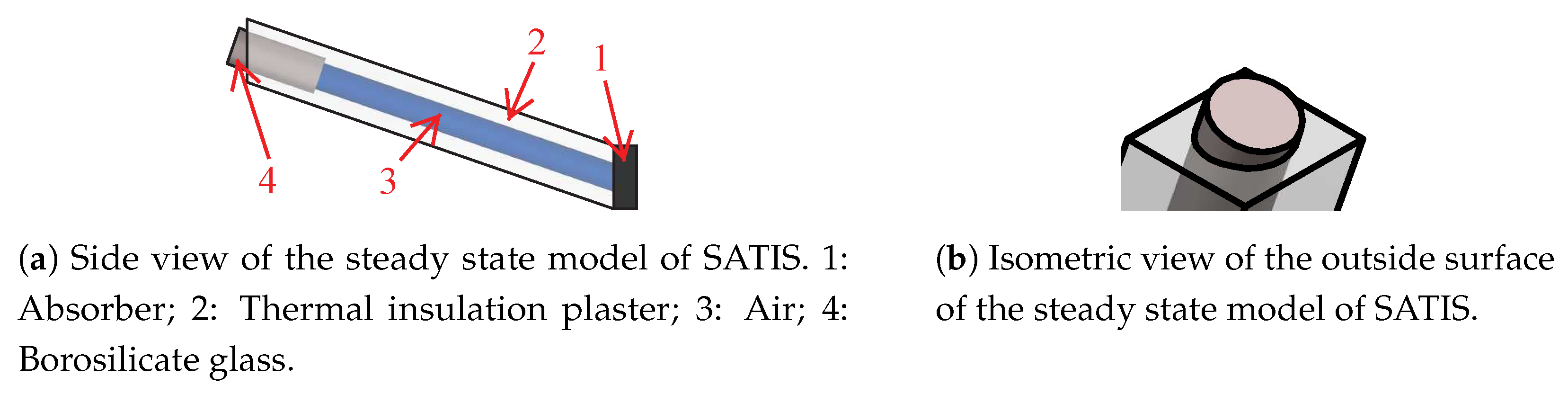
2.1. Reference Model of the Solar Selective Thermal Insulation System (SATIS)

The steady state model of SATIS, which was developed with COMSOL Multiphysics^® and thoroughly validated and described in [17], is shown in Figure 1a,b in side and isometric view, respectively. The model consists of a single light conducting element (LCE). SATIS comprises the micro hollow glass spheres thermal insulation plaster (2) [21,22], air (3) and borosilicate glass (4) [23]. The solar radiation entering the LCE from the outside (left in Figure 1a) through the borosilicate glass cylinder acting as a closure element (4) is absorbed by the absorber plate (1) consisting of a black painted steel sheet. The front diameter ($d_1$) stays for the closure element (4), while the rear diameter ($d_2$) for the air-filled part (3) of the LCE. The axis of the stepped hole of the LCE is inclined at an angle of 19° to the horizontal, so that solar gains can be obtained preferably in winter months. For solar radiation incident at this angle, the highest total solar energy transmittance could be determined both experimentally (11.2%) and numerically (11.7%) [17].

2.2. Parameter Sensitivity Analysis

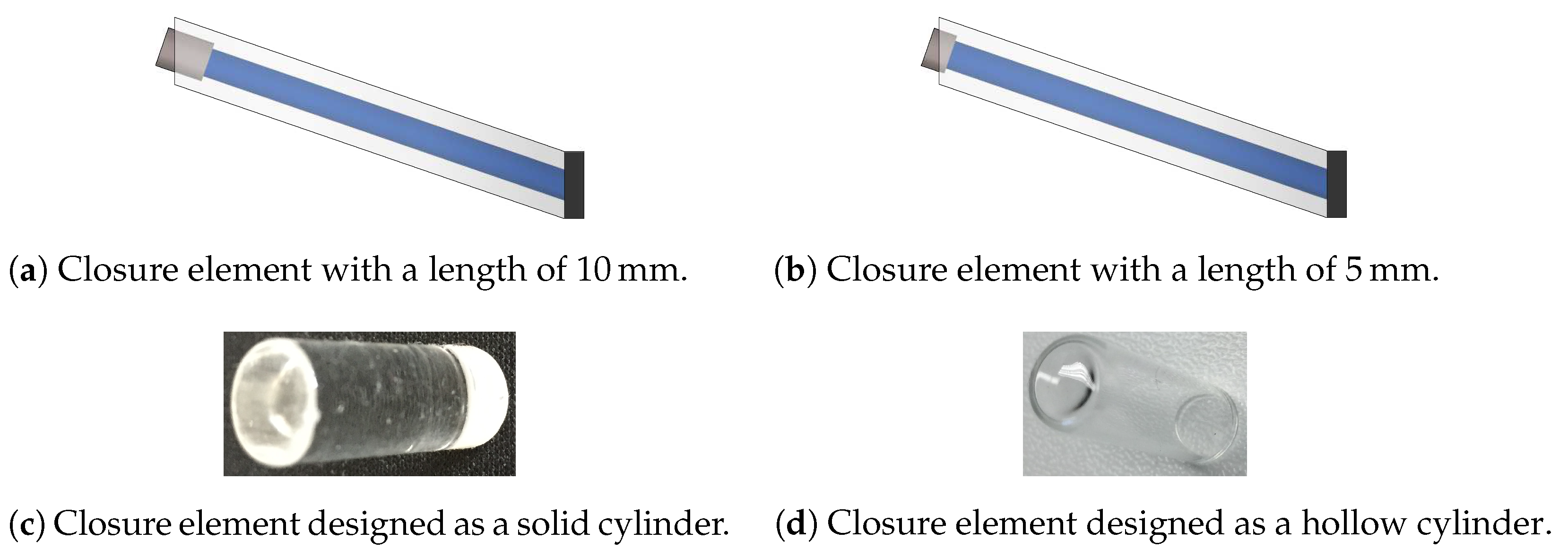
The model described in Section 2.1 serves as reference for the parameter sensitivity analysis of SATIS. To evaluate the influence of the construction parameters on the insulating performance and the solar gain, the effective thermal conductivity (${\lambda }_{\mathrm{eff}}$) and the angle-dependent total solar energy transmittance (g) are used. In this study, the influence of the following parameters on ${\lambda }_{\mathrm{eff}}$ and g is investigated:

• Length ($L_{\mathrm{glass}}$) and shape (solid/hollow cylinder) of the closure element.
• Short-wave absorption coefficient of the absorber (${\alpha }_{\mathrm{abs}}$).
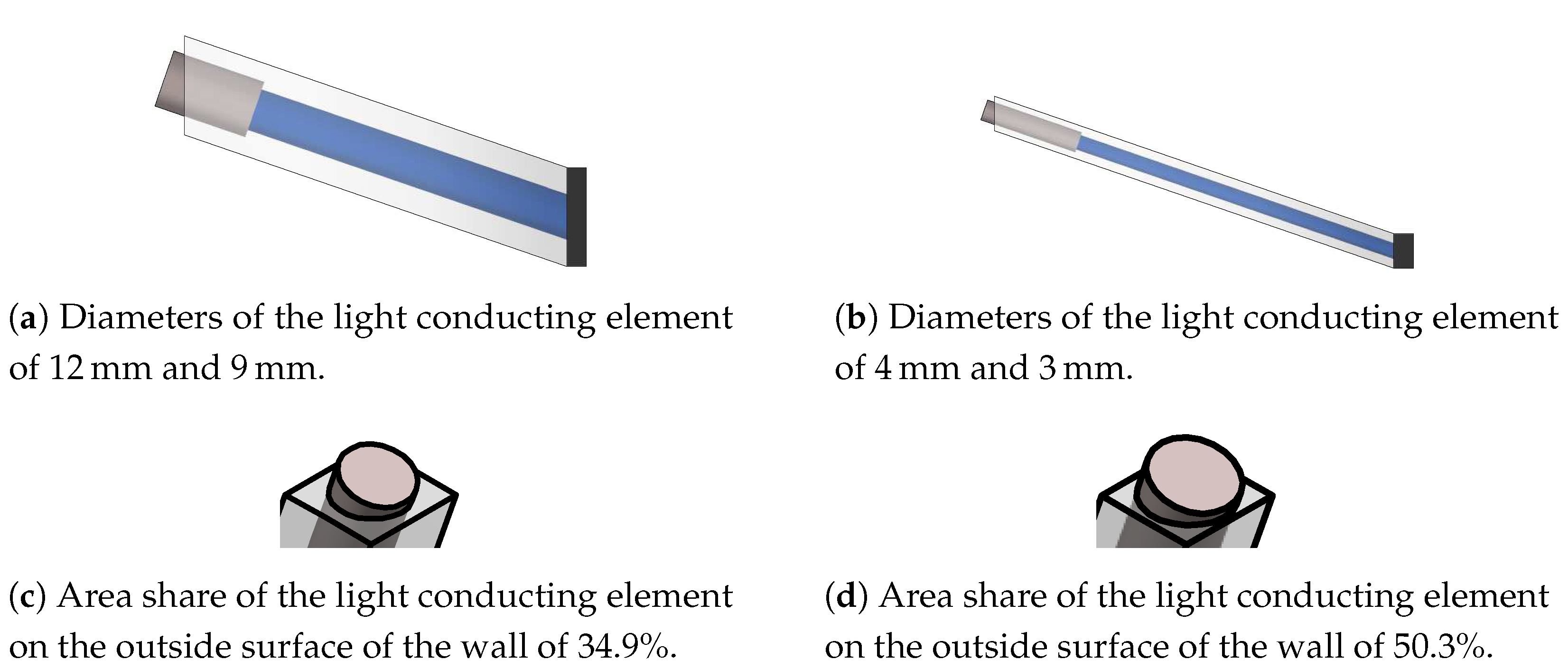
• Front and rear diameter of the stepped hole ($d_1$/$d_2$) of the light conducting element.
• Area share of the LCE on the outside surface of the wall ($A_{\mathrm{LCE}}$).
• Alignment of the incident light rays (solar simulator from the experimental investigations with ±2° alignment deviation [17,20] or absolutely aligned light rays).

The first two investigated parameters are related to the closure element, which is, in the first prototype of SATIS, designed as a solid cylinder made of borosilicate glass with a length of 20 mm. The disadvantage of this transparent closure element is its action as a thermal bridge element, which has already been shown in [17]. Since the thermal conductivity of glass (1.2 $\frac{\mathrm{W}}{\mathrm{mK}}$ [23]) is significantly higher than that of the thermal insulation plaster and air, the overall thermal resistance of the insulation layer is reduced. Based on the calculated effective thermal conductivity of the SATIS prototype (56.1 $\frac{\mathrm{mW}}{\mathrm{mK}}$ [17]), the thermal insulation performance must be increased to achieve a similar thermal resistance as the thermal insulation plaster without LCEs ((45 ± 2) $\frac{\mathrm{mW}}{\mathrm{mK}}$ [17,20]). For this reason, heat and radiation transport studies are performed for cylinder lengths of 10 mm (cf. Figure 2a) and 5 mm (cf. Figure 2b), respectively. In addition, the effect of the shape of the closure element is also numerically investigated. Therefore, as an alternative to the solid cylinder (cf. Figure 2c), an investigation using a hollow cylinder with a wall thickness of 1 mm (cf. Figure 2d) is carried out.

The third construction parameter is related to the absorber, on which SATIS is applied. In the experiments and for the developed steady state model, a black painted steel plate was used. The black coloring is intended to absorb the short-wave radiation transported through the light conducting element as effectively as possible. In this study, the short-wave absorption coefficient (${\alpha }_{\mathrm{abs}}$) is varied between 60% and 90% to verify the need for a black absorber surface when applying SATIS.

Regarding the diameters of the LCE ($d_1$/$d_2$), starting from the prototype with diameters of 8 mm/6 mm, a sensitivity analysis is performed for 12 mm/9 mm (cf. Figure 3a) and 4 mm/3 mm (cf. Figure 3b). The diameters were chosen in such a way that the area ratio of the diameters remains constant (${12}^2/9^2=8^2/6^2=4^2/3^2$), but a variation of the $L/D$ ratio occurs, since the layer thickness of SATIS remains constant at $L=80 \mathrm{m}\mathrm{m}$. When varying the diameters, the influence of the alignment of the incident light rays is also investigated. In contrast to the investigations in [17], in which the light rays have an alignment deviation of ±2° due to the solar simulator, absolutely aligned light rays are used. Furthermore, the influence of the area share of the LCE on the outside surface of the wall ($A_{\mathrm{LCE}}$) on ${\lambda }_{\mathrm{eff}}$ and g, starting from the prototype (26.4%), is examined for $A_{\mathrm{LCE}}$ of 34.9% (cf. Figure 3c) and 50.3% (cf. Figure 3d), respectively.

Table 1. Investigated variants in the parameter study.

Variant	${\mathit{L}}_{\mathbf{glass}}$ in mm	Shape	${\mathit{\alpha }}_{\mathbf{abs}}$ in %	${\mathit{d}}_1$/${\mathit{d}}_2$ in mm/mm	${\mathit{A}}_{\mathbf{LCE}}$ in %	Ray Alignment in °
Reference	20	solid	90	8/6	26.4	$\pm 2$
V1	5	solid	90	8/6	26.4	$\pm 2$
V2	10	solid	90	8/6	26.4	$\pm 2$
V3	20	hollow	90	8/6	26.4	$\pm 2$
V4	5	hollow	90	8/6	26.4	$\pm 2$
V5	10	hollow	90	8/6	26.4	$\pm 2$
V6	20	solid	60	8/6	26.4	$\pm 2$
V7	20	solid	70	8/6	26.4	$\pm 2$
V8	20	solid	80	8/6	26.4	$\pm 2$
V9	20	solid	90	4/3	26.4	$\pm 2$
V10	20	solid	90	12/9	26.4	$\pm 2$
V11	20	solid	90	8/6	26.4	$\pm 0$
V12	20	solid	90	4/3	26.4	$\pm 0$
V13	20	solid	90	12/9	26.4	$\pm 0$
V14	20	solid	90	8/6	34.9	$\pm 2$
V15	20	solid	90	8/6	50.3	$\pm 2$

summarizes all investigated parameter configurations.

2.3. Yearly Simulation Models

The assessment of the actual energy savings of the solar selective thermal insulation system is performed through the comparison with a wall construction insulated with the the same thermal insulation plaster but without SATIS (“conventional wall construction”). Here, two different variants of SATIS are compared with this construction in a one year transient study with respect to winter energy transmission losses and summer heat gains.

The common feature of the investigated models is that the south-oriented wall constructions, which are visualized in Figure 4a–c, have the same basic structure consisting of interior plaster (1.5 cm [24]), solid brickwork (36.5 cm [20]) and adhesive plaster blackened with iron oxide (0.5 cm [25,26]). Except for the shorter glass cylinder (10 mm instead of 20 mm), the SATIS #1 variant in Figure 4b has the same properties as the fabricated and experimentally investigated prototype [17]. SATIS #2 in Figure 4c represents a modified variant considering construction improvements derived from the parameter sensitivity analysis.

Table 2. Main physical and construction properties of the yearly simulation models from Figure 4.

Model	${\mathit{d}}_1$/${\mathit{d}}_2$ in mm/mm	${\mathit{A}}_{\mathbf{LCE}}$ in %	${\mathit{L}}_{\mathbf{glass}}$ in mm	${\mathit{\lambda }}_{\mathbf{eff},\mathbf{insul}.}$ in $\frac{\mathbf{mW}}{\mathbf{mK}}$	${\mathit{U}}_{\mathbf{cond}+\mathbf{rad}}$/${\mathit{U}}_{\mathbf{cond}}$ in $\frac{\mathbf{W}}{\mathbf{m}{}^2\mathbf{K}}$
Conv.	-	-	-	45.0	-/0.399
SATIS #1	8/6	26.4	10	48.9	0.424/0.396
SATIS #2	12/9	44.2	10	53.7	0.452/0.382

lists the main physical and construction properties of the investigated wall configurations. Compared to the insulation layer of the investigated SATIS prototype (56.1 $\frac{\mathrm{mW}}{\mathrm{mK}}$ [17]), the insulation layers of the solar selective wall constructions #1 and #2 show effective thermal conductivities of 48.9 $\frac{\mathrm{mW}}{\mathrm{mK}}$ and 53.7 $\frac{\mathrm{mW}}{\mathrm{mK}}$, respectively.

Regarding the solar selective wall constructions, the heat transfer mechanisms within the LCE, conduction (cond) and long-wave thermal radiation (rad) are vital for the calculation of ${\lambda }_{\mathrm{eff}}$ of SATIS and the U-value of the entire wall construction, respectively, as shown in [17]. However, the integration of long-wave thermal radiation in the transient numerical model, compared to the sole calculation of conduction, results in an unreasonably prolonged calculation time. According to an extrapolation carried out from short-time computations, calculation time increases by a factor of 13 when long-wave radiation is taken into account in the simulation model. This implies a computation time of 4062.5 h (169 days) instead of 312.5 h (13 days). Therefore, the calculations in this study were performed solely taking into account conduction. Nevertheless, in order to consider the actual heat losses due to conduction and thermal radiation ($q_{\mathrm{cond}+\mathrm{rad}}$), the numerically computed yearly energy losses due to conduction ($q_{\mathrm{cond}}$) are scaled with the ratio of the steady state U-values ($U_{\mathrm{cond}+\mathrm{rad}}/U_{\mathrm{cond}}$, cf. Table 2) according to Equation (1). Equation (1) is valid for long time periods (e.g., heating period), since the steady state heat loss depends solely on the applied temperature difference between the indoor and outdoor air and the U-value. Since the same air temperature differences are applied (same ambient air test data), there is only a dependence of the heat loss on the U-value of the wall construction.

$$q_{\mathrm{cond}+\mathrm{rad}}=q_{\mathrm{cond}}\frac{U_{\mathrm{cond}+\mathrm{rad}}}{U_{\mathrm{cond}}}$$

(1)

For the calculation of the steady state U-values in Table 2, the standard heat transfer coefficients [27] on the inside and outside surfaces of the wall of 7.69 $\frac{\mathrm{W}}{{\mathrm{m}}^2\mathrm{K}}$ and 25 $\frac{\mathrm{W}}{{\mathrm{m}}^2\mathrm{K}}$ were used, respectively. Compared with the numerical investigations for the validation of the steady state model in [17], it is also necessary to take into account the smaller alignment deviation of the light rays of the sun (±0.2666°) compared with that of the solar simulator (±2°).

The test data shown in Figure 5a, consisting of ambient air temperature ($T_{\mathrm{ambient}}$) and direct radiation on a surface perpendicular to the direction of irradiation (derived from direct radiation on a horizontal surface (${\dot{q}}_{\mathrm{direct},\mathrm{horizontal}}$)), are the boundary conditions on the outside surfaces of the models. This data set was created from the hourly climatic data of Nürnberg (station id: 03668) for the year 2018 [28]. The test data set starts on the 16.09.2018 (t = 0 h). A year-round indoor air temperature of 21 °C is applied for all models, so that both winter energy transmission losses and summer overheating effects can be directly compared between the investigated wall constructions.

Figure 5b shows the daily mean ambient air temperature (${\overline{T}}_{\mathrm{ambient}}$) of the test data set and the heating threshold temperatures of 10 °C and 15 °C [29], respectively, which are used to estimate the length of the heating period. If the daily mean ambient air temperature is lower than these threshold temperatures, a heat loss calculation is performed for the resulting heating period. Figure 5b shows the periods 22.09.–20.05. (15 °C) and 21.10.–03.04. (10 °C), which are used for comparing the simulation models.

The physical quantity used for the assessment of the actual energy losses is the heat flux on the inside surface of each wall construction (${\dot{q}}_{\mathrm{IS}}$). The objective during the heating season is to minimize the heat flux that is dissipated from the indoor space and thus must be supplied via other means (e.g., fossil fuels) to maintain a constant indoor air temperature of 21 °C. This shall be accomplished by solar energy transmitted through the LCE from the outside to the inside surface of the wall. The transmitted energy increases the temperature on the absorber surface behind SATIS and, accordingly, reduces or even changes the sign of the temperature difference for the transmission heat losses, resulting in decreasing the heat loss or even realizing a heat gain. Equation (2) defines the area-specific amount of heat loss from the inside wall ($q_{\mathrm{IS}}^{t_1\to t_2}$) in the considered period ($t_1$ to $t_2$, e.g., 22.09.–20.05.) as an integral comparison parameter between the different wall constructions from Figure 4 and Table 2.

$$q_{\mathrm{IS}}^{t_1\to t_2}={\int }_{t_1}^{t_2}{\dot{q}}_{\mathrm{IS}}\mathrm{d}t$$

(2)

The coupled computation of the heat and short-wave radiation transport in the steady state model in [17] was limited to a one-time computation of the radiation distribution by ray tracing, which was subsequently considered constant in the thermal simulation. Due to the temporally varying position of the sun in the transient simulation, the computationally intensive ray tracing simulation would have to be performed again after an infinitesimally small time step, taking into account the instantaneous solar radiation intensity as well as the associated polar angle ($\phi \left(t\right)$) and azimuth ($\psi \left(t\right)$) of the sun. Since the weathering data are hourly averaged, only one mean radiation distribution is determined for each hour from a linear interpolation of the solar position present at the beginning and the end of that hour as well the corresponding solar radiation intensity. This procedure is shown in Figure 6a. Here, the radiation distribution on the outside surface of the wall or in the LCE is calculated from the mean measured radiation intensity in the period from $X_I$ to $X_{II}$ and the polar angle and azimuth of $X_i$. A similar procedure is used for the outdoor air temperature ($T_{\mathrm{ambient}}$) shown in Figure 6b, in which the states are labeled $Y_I$, $Y_{II}$, and $Y_i$.

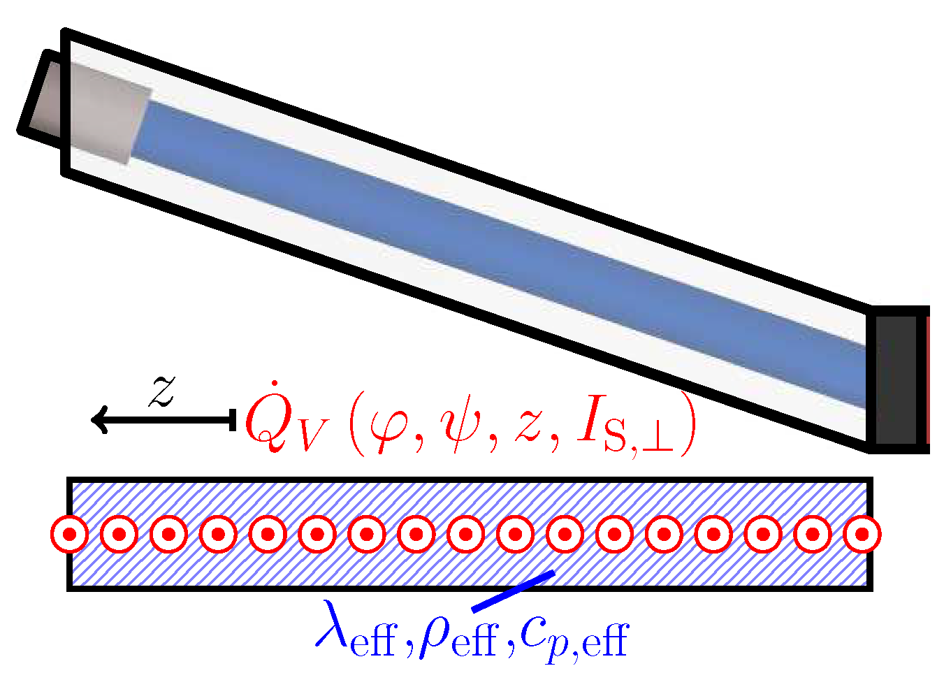
2.4. Simplified Computational Methodology for 1D Simulation Tools

The ray tracing methodology presented in Section 2.3 based on the model introduced in [17] computes the radiation distribution in the LCE for each mean solar position, which subsequently serves as an input variable for the dynamic heat transfer simulation. Common building simulation software, such as WUFI^® or IDA ICE, often uses one-dimensional model equations [30,31,32] without any ray tracing simulation capability to compute the heat transport in wall structures. Therefore, in order to utilize the solar selective properties of SATIS in 1D simulation tools, a simplified computational methodology is required. The basis of the developed methodology is the extension of the one-dimensional transient conduction differential equation by the heat source term (${\dot{Q}}_V$) as defined in Equation (3).

$$\rho c_p\frac{\partial T}{\partial t}=\frac{\partial }{\partial z}\left(\lambda \frac{\partial T}{\partial z}\right)+{\dot{Q}}_V\left(\phi \left(t\right),\psi \left(t\right),z,I_{\mathrm{S},\perp }\left(t\right)\right)$$

(3)

In Equation (3), $\rho$ denotes density, $c_p$ specific heat capacity, T temperature, t time, z spatial coordinate, $\lambda$ thermal conductivity, $\phi$ polar angle, $\psi$ azimuth and $I_{\mathrm{S},\perp }$ solar radiation intensity on a surface perpendicular to the direction of irradiation. ${\dot{Q}}_V$ is applied in the insulation layer to account for the heat fluxes occurring in the LCE due to solar radiation. Figure 7 illustrates the LCE of the simulation model SATIS #1 (top) and the one-dimensional representation of the insulation layer (bottom). This layer uses effective values for thermal conductivity (${\lambda }_{\mathrm{eff}}$), density (${\rho }_{\mathrm{eff}}$), and specific heat capacity ($c_{p,\mathrm{eff}}$).

Regarding the heat source modeling, the dependencies of ${\dot{Q}}_V$ on the position within the LCE (z), the time and the instantaneous solar position parameters deriving from it ($\phi \left(t\right)$ and $\psi \left(t\right)$), as well as the current solar radiation intensity perpendicular to the direction of irradiation ($I_{\mathrm{S},\perp }\left(t\right)$) have to be considered. Thus, in principle, a function of four independent quantities is used, i.e., ${\dot{Q}}_V={\dot{Q}}_V\left(\phi \left(t\right),\psi \left(t\right),z,I_{\mathrm{S},\perp }\left(t\right)\right)$. To determine this functional relationship, the independent variables are first reduced from four to three. This can be achieved by scaling (multiplying by the scaling factor $\mathrm{SF}$) the actual solar radiation intensity ($I_{\mathrm{S},\perp }\left(t\right)$) with respect to a reference condition ($I_{\mathrm{S},\perp ,\mathrm{ref}}$) according to Equation (4). This approach is based on the premise that the radiation distribution within the LCE remains the same, except that there is locally a proportional ($\mathrm{SF}$) change in the heat flux.

$${\dot{Q}}_V\left(\phi \left(t\right),\psi \left(t\right),z,I_{\mathrm{S},\perp }\left(t\right)\right)=\underset{\mathrm{SF}}{\underbrace{\frac{I_{\mathrm{S},\perp }\left(t\right)}{I_{\mathrm{S},\perp ,\mathrm{ref}}}}}{\dot{Q}}_V\left(\phi \left(t\right),\psi \left(t\right),z,I_{\mathrm{S},\perp ,\mathrm{ref}}\right)$$

(4)

In this study, a radiant heat flow map is generated from these three independent quantities at the reference intensity ($I_{\mathrm{S},\perp ,\mathrm{ref}}$) of 1000 $\frac{\mathrm{W}}{{\mathrm{m}}^2}$. This map is determined by means of a ray tracing simulation in step sizes of $\mathsf{\Delta }\phi =\mathsf{\Delta }\psi =2°$ and $\mathsf{\Delta }z=5 \mathrm{m}\mathrm{m}$. In general, the instantaneous incidence angles ($\phi$ and $\psi$) do not coincide with the determined grid points, so that an interpolation must be performed. Indeed, the accuracy of this interpolation increases with decreasing every step size.

3. Results and Discussion

In this section, the influence of the construction parameters on the effective thermal conductivity (${\lambda }_{\mathrm{eff}}$) and the total solar energy transmittance (g) is presented. Furthermore, the yearly energy balances of the solar selective wall constructions #1 and #2 are compared with that of the wall structure insulated with the same thermal insulation plaster and thickness, but without SATIS (“conventional wall construction”).

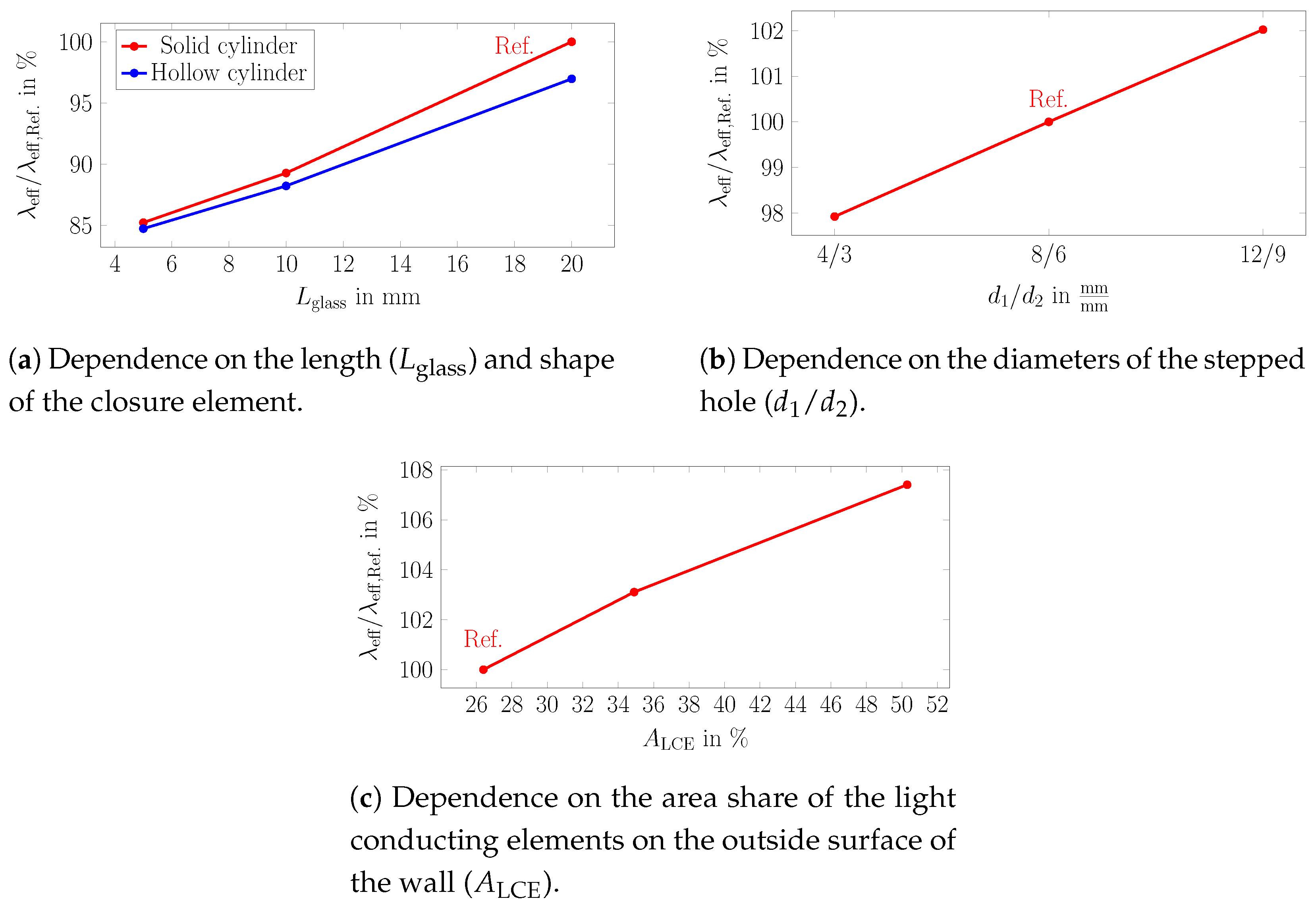
3.1. Influence of the Construction Parameters on the Effective Thermal Conductivity

One main objective of the design review of SATIS is to reduce its effective thermal conductivity as much as possible to ensure sufficient thermal protection, especially on days with no solar irradiation. To this aim, the reference model from Figure 1 is applied to study the effect of the varied design parameters according to Table 1 on reducing the effective thermal conductivity. Figure 8a–c show, starting from the reference condition (Ref.), which has the listed parameters in line one of Table 1, the change in the effective thermal conductivity versus the length and shape of the closure element (a), the diameters of the stepped hole (b) and the area share of the LCE on the outside surface of the wall (c).

As shown in Figure 8a, a reduction in the glass cylinder length ($L_{\mathrm{glass}}$), regardless of shape, leads to a decrease in the effective thermal conductivity. Reducing the length of the solid cylinder from 20 mm to 5 mm results in reducing the reference effective thermal conductivity by −14.8%. This can be attributed to the fact that reducing the penetration depth of the glass element increases the overall thermal resistance, since this more conductive closure element is replaced by a combination of air and thermal insulation plaster, which have significantly lower thermal conductivities. The use of a hollow instead of a solid cylinder shows only a slight improvement. The largest reduction of −3.1% occurs at the reference length of 20 mm. Even with a hollow cylinder and a wall thickness of only 1 mm, the glass cross-sectional area is still 43.8% of the solid cylinder. Therefore, the thermal bridge effect is still present with the net effect of lowering the thermal resistance in the front region. As the hollow glass cylinder length is reduced, the difference between solid and hollow material in terms of effective thermal conductivity decreases and nearly diminishes for the cylinder length of 5 mm.

The influence of the diameters of the stepped hole ($d_1$/$d_2$) on the effective thermal conductivity from Figure 8b is only of minor importance compared to the variation of the glass cylinder length. As the L/D ratio decreases (increasing hole diameters), ${\lambda }_{\mathrm{eff}}$ increases slightly because the influence of long-wave thermal radiation within the holes becomes more significant. Reducing the diameters to 4 mm/3 mm, ${\lambda }_{\mathrm{eff}}$ can be lowered by −2.1% compared to the reference design. A stronger influence is observed, however, when varying the area share of the LCE on the outside surface ($A_{\mathrm{LCE}}$), as depicted in Figure 8c. Here, the increase in effective thermal conductivity correlates with increasing the area share of the LCE. This can be attributed mainly to the growing proportion of glass (thermal bridge) within SATIS.

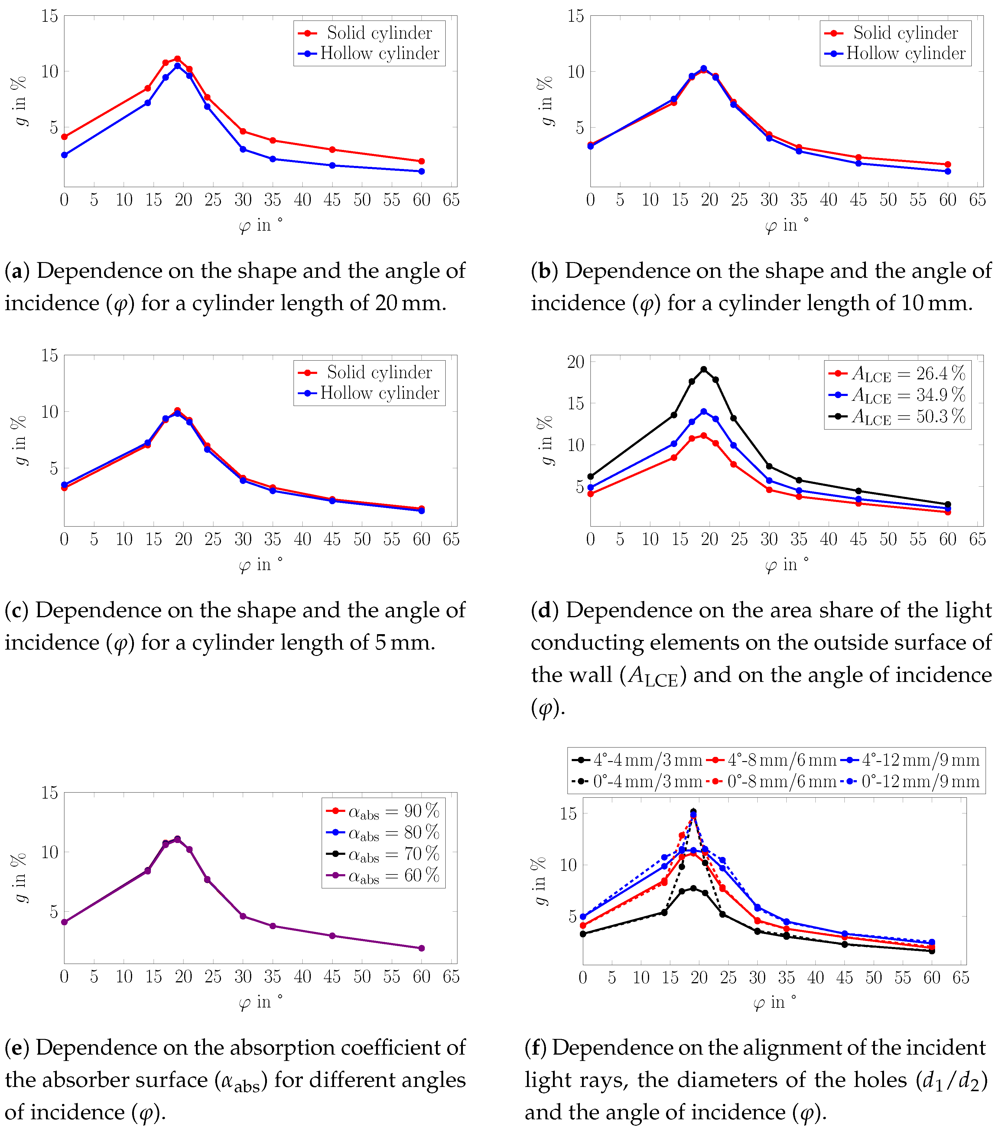
3.2. Influence of the Construction Parameters on the Total Solar Energy Transmittance

The total solar energy transmittance (g) is used to evaluate the impact of the construction parameters on the winter and summer solar heat gains. Figure 9a–c show the dependence of g on the shape for cylinder lengths of 20 mm, 10 mm and 5 mm. Two trends can be identified in these figures. With decreasing cylinder length, there is a slight reduction of g for each shape of about −1% at the design angle, which is due to the axial shift of the transition zone of the hole diameters (8 mm to 6 mm) and, correspondingly, different positions of absorption. Furthermore, the difference in g, similar to the effective thermal conductivity in Figure 8a, decreases between solid and hollow cylinders with reduced cylinder length. According to the obtained results, the closure element has only a minor overall influence on the total solar energy transmittance, but as shown in Section 3.1, the shortening of the glass cylinder can strongly reduce ${\lambda }_{\mathrm{eff}}$.

Considering the influence of the area share of the LCEs ($A_{\mathrm{LCE}}$) on the total solar energy transmittance (cf. Figure 9d), in particular for irradiation angles with small deviations around the design angle (19°), significantly higher solar gains can be achieved with increasing the area share of the LCEs. For 19°, changing $A_{\mathrm{LCE}}$ from 26.4% to 50.3% leads to an increase in g from 11.7% to 19.1%. This is particularly advantageous during winter solar irradiation, as it allows the transmission heat losses to be counteracted to a greater extent by the higher solar gains. At higher incidence angles (e.g., 60°), even with an area share of 50.3%, there is only a 1% higher total solar energy transmittance compared with 26.4% (2.9% vs. 1.9%). This can be attributed to the fact that the solar radiation is absorbed primarily in the front area and is emitted directly to the ambient. Thus, an increased area share of the LCEs has a positive effect on the winter solar energy gain without having a significant negative effect on summer overheating protection. However, this positive effect of increasing $A_{\mathrm{LCE}}$ is accompanied by a negative effect on the effective thermal conductivity (cf. Figure 8c). Accordingly, no general recommendation can be made here to always increase this value, as the higher transmission heat losses may not be compensated by the additional solar gains. In order to judge on this parameter, the annual energetic assessment of the whole wall construction as described in Section 2.3 is needed.

The influence of varying the absorption coefficient of the absorber layer (${\alpha }_{\mathrm{abs}}$) on the total solar energy transmittance over the studied range of incidence angles is visualized in Figure 9e. As can be observed, the variation of ${\alpha }_{\mathrm{abs}}$ has a negligible effect on the total solar energy transmittance for all incidence angles. For larger deviations from 19°, most of the incident solar radiation is absorbed near the outside surface of the wall. Accordingly, there is no influence of ${\alpha }_{\mathrm{abs}}$ on g. The explanation for the negligible effect of ${\alpha }_{\mathrm{abs}}$ on g at or around the design angle of 19° is quite different. Indeed, the radiation striking the absorber area is partially absorbed and partially reflected based on the absorption coefficient. Due to the very small diameter of 6 mm, for the investigated reference design, almost the whole diffusely reflected radiation is absorbed by the insulation material surface surrounding the LCE in the immediate vicinity of the absorber. Recalling that the total solar energy transmittance is evaluated under steady state conditions, the net heat flux is not directly received through the LCE by radiation, but indirectly through the insulation material itself by conduction. At enlarged diameters of the LCE, it is expected that a greater portion of the reflected radiation by the absorber may propagate further to the outside surface of the wall and, consequently, the influence of the absorption coefficient on the total solar energy transmittance would be stronger.

Figure 9f shows the total solar energy transmittance (g) for the diameter ratios of 12 mm/9 mm, 8 mm/6 mm and 4 mm/3 mm. In this investigation, compared to the parameter studies illustrated in Figure 9a–e, which were computed for the alignment deviation of the light rays of the solar simulator (±2°), a variation of this alignment is also performed (perfectly aligned light rays). As can be seen in Figure 9f, especially at the design angle of 19° and in its close vicinity, a higher total solar energy transmittance is obtained for all diameters with increasing the alignment of the light rays. Furthermore, irrespective of the alignment of the light rays, the highest total solar energy transmittances are obtained near the design angle for the lowest investigated L/D ratio (12 mm/9 mm). The influence of the L/D ratio can be also observed for larger deviations of the incidence angle from 19°, where again lower ratios allow for higher total solar energy transmittances, since overall, there are fewer reflections of the light rays at the walls of the LCE on their way to the absorber. For high incidence angles (e.g., 60°), similar to the behavior by varying $A_{\mathrm{LCE}}$, a significant reduction of the differences in g between the investigated diameters occurs, which contributes to summer overheating protection. In general, it must also be taken into account that although higher solar gains are possible with decreasing L/D ratio, this also increases the influence of natural convection and long-wave thermal radiation inside the LCE (higher ${\lambda }_{\mathrm{eff}}$, cf. Figure 8b).

3.3. Yearly Energetic Performance of the Solar Selective Thermal Insulation System (SATIS)

The numerical simulations for computing the yearly energetic performance start on the date 16.09. with the steady state initial temperature distribution within each wall construction. Thus, each simulation model has a settling time of about one week before the first evaluation period (heating threshold temperature of 15°) starts on 22.09. Figure 10 shows, starting from 22.09. (t = 0 h), the temperature in the absorber or behind the insulation layer ($T_{\mathrm{abs}}$) for the investigated wall constructions.

It can be observed that $T_{\mathrm{abs}}$ of the solar selective wall constructions #1 and #2 is subjected to significantly stronger fluctuations in autumn and especially in winter months than in summer. This is due to the solar gains at lower incidence angles, which result in an increase in the absorber temperature. During summer, absorption occurs primarily in the front area of the LCE. Due to the higher absorption coefficient of the plaster in the LCE compared with that of the exterior white wall paint of the wall construction insulated with the same thermal insulation plaster but without SATIS (“Conventional”), $T_{\mathrm{abs}}$ of the solar selective wall constructions is a little higher than the temperature behind the insulation layer of the conventional system during summer. Particularly at low daily mean air temperatures in the order of −10 °C and at the same time comparatively high solar radiation intensities (cf. Figure 5 day 166 or hour 3800), the solar selective wall construction #2 has an approximately 2.2 K higher average temperature in the absorber compared with the conventional wall construction.

Figure 11 shows the heat flux on the inside surface of the wall (${\dot{q}}_{\mathrm{IS}}$) for the conventional wall construction and the solar selective variants #1 and #2. Positive heat fluxes correspond to a heat flow towards the outside surface of the wall, i.e., a transmission heat loss. Comparing the wall constructions with each other, solar gains in the middle of October (hour 560) are obtained for the wall construction #2. Here, the temperature on the inside surface of the wall exceeds the indoor air temperature of 21 °C, releasing heat to the indoor space (${\dot{q}}_{\mathrm{IS}}<0 \frac{\mathrm{W}}{{\mathrm{m}}^2}$). Even in winter months, a reduction in the heat flux is achieved for certain days if a suitable incidence angle and sufficient solar radiation are available. The maximum heat loss can be reduced by about 25% with the solar selective wall construction #2 at the lowest daily mean air temperature (early March, hour 3800) compared with the conventional wall construction (from 11.4  $\frac{\mathrm{W}}{{\mathrm{m}}^2}$ to 8.4  $\frac{\mathrm{W}}{{\mathrm{m}}^2}$).

Examining the heat flux released into the indoor space (${\dot{q}}_{\mathrm{IS}}<0 \frac{\mathrm{W}}{{\mathrm{m}}^2}$) during the summer months (21.05.–21.09., hour 5784 to 8760) in Figure 12, there is only a slight shift of the curves of the solar selective wall constructions towards lower heat fluxes, i.e., higher heat gains into the interior occur. A large amount of heat is absorbed near the closure element and immediately transferred back into the ambient. The heat input into the solid brickwork or the heat transport to the inside of the wall occurs almost exclusively by thermal diffusion processes in the LCE, so that no significant peak heat flows occur as opposed to the winter months.

Figure 13 illustrates the evaluation of Equation (2) to determine the area-specific amount of heat on the inside surface of the wall and is performed for the periods 22.09.–20.05. (heating threshold temperature 15°), 21.10.–03.04. (heating threshold temperature 10°) and 21.05.–21.09. (summer months) for the wall construction insulated with the same thermal insulation plaster, but without SATIS (“Conventional”) and the solar selective variants #1 and #2. The conventional wall construction has heat losses due to conduction (HL cond) of $q_{\mathrm{IS}}^{\mathrm{22.09.}\to \mathrm{20.05.}}=31.82 \frac{\mathrm{k}\mathrm{W}\mathrm{h}}{{\mathrm{m}}^2}$/$q_{\mathrm{IS}}^{\mathrm{21.10.}\to \mathrm{03.04.}}=27.17 \frac{\mathrm{k}\mathrm{W}\mathrm{h}}{{\mathrm{m}}^2}$. For the solar selective wall constructions #1 and #2, these heat losses amount to only 28.84 $\frac{\mathrm{k}\mathrm{W}\mathrm{h}}{{\mathrm{m}}^2}$/25.22 $\frac{\mathrm{k}\mathrm{W}\mathrm{h}}{{\mathrm{m}}^2}$ and 23.71 $\frac{\mathrm{k}\mathrm{W}\mathrm{h}}{{\mathrm{m}}^2}$/21.76 $\frac{\mathrm{k}\mathrm{W}\mathrm{h}}{{\mathrm{m}}^2}$, respectively.

However, the increased transmission heat losses due to long-wave thermal radiation (HL cond+rad), as mentioned in Section 2.3, must be taken into account by means of the U-value ratio according to Equation (1). This results in effective heat losses for the solar selective wall constructions #1 and #2 of 30.88 $\frac{\mathrm{k}\mathrm{W}\mathrm{h}}{{\mathrm{m}}^2}$/27 $\frac{\mathrm{k}\mathrm{W}\mathrm{h}}{{\mathrm{m}}^2}$ and 28.06 $\frac{\mathrm{k}\mathrm{W}\mathrm{h}}{{\mathrm{m}}^2}$/25.75 $\frac{\mathrm{k}\mathrm{W}\mathrm{h}}{{\mathrm{m}}^2}$, respectively. Therefore, SATIS #1 has absolute and relative effective solar gains (SG) of 0.94 $\frac{\mathrm{k}\mathrm{W}\mathrm{h}}{{\mathrm{m}}^2}$/0.17 $\frac{\mathrm{k}\mathrm{W}\mathrm{h}}{{\mathrm{m}}^2}$ and 3.0%/0.6%, respectively, compared with the conventional wall construction. SATIS #2, which already incorporates construction improvements from the parameter sensitivity analysis in Section 2.2, enables a reduction of 3.76 $\frac{\mathrm{k}\mathrm{W}\mathrm{h}}{{\mathrm{m}}^2}$/1.42 $\frac{\mathrm{k}\mathrm{W}\mathrm{h}}{{\mathrm{m}}^2}$ and 11.8%/5.2%, respectively. To balance the additional cooling energy required to maintain the indoor air temperature of 21 °C compared to the conventional wall, the negative heat fluxes shown in Figure 12 are used during the period 21.05.–21.09. (hour 5784 to 8760). Effective overheating values (OH) of 0.43 $\frac{\mathrm{k}\mathrm{W}\mathrm{h}}{{\mathrm{m}}^2}$ (#1) and 1.29 $\frac{\mathrm{k}\mathrm{W}\mathrm{h}}{{\mathrm{m}}^2}$ (#2), compared to the conventional system, are obtained here. Thus, in absolute terms, improving the construction from #1 to #2 can increase the solar gain (SG) by 2.82 $\frac{\mathrm{k}\mathrm{W}\mathrm{h}}{{\mathrm{m}}^2}$/1.25 $\frac{\mathrm{k}\mathrm{W}\mathrm{h}}{{\mathrm{m}}^2}$, while the overheating (OH) rises only by 0.86 $\frac{\mathrm{k}\mathrm{W}\mathrm{h}}{{\mathrm{m}}^2}$.

The methodology presented in Section 2.4 using a one-dimensional model of the wall structure and a radiant heat flow map to account for the heat fluxes occurring in the LCE is evaluated below. Figure 14 shows the map for $I_{\mathrm{S},\perp ,\mathrm{ref}}=1000\frac{\mathrm{W}}{{\mathrm{m}}^2}$ with $0°\le \phi \le 66°$, $0°\le \psi \le 88°$ and $0 \mathrm{m}\le z\le 0.08 \mathrm{m}$, which was calculated for step sizes of $\mathsf{\Delta }\phi =\mathsf{\Delta }\psi =2°$ and $\mathsf{\Delta }z=5 \mathrm{m}\mathrm{m}$. This map, which is exclusively valid for the solar selective wall construction #1, was determined through a ray tracing simulation. Since the present investigations involve a south-facing facade, the calculation of half the map is sufficient, since there is a symmetrical radiation distribution about the $\phi$-axis. The color coding in Figure 14 also takes into account the comparatively high heat fluxes (large surface area) occurring on the outside surface of the wall ($z=0.08 \mathrm{m}$), so that a large amount of grid points in Figure 14 lies in the lower range of the color coding. However, on the $\phi$-axis ($\psi =0°$), the penetration of the short-wave radiation towards the absorber ($z=0 \mathrm{m}$) in the immediate vicinity of the design angle ($\phi =19°$) is well visible.

The computed radiant heat fluxes are used in the heat source term in Equation (3). Moreover, the scaling factor from Equation (4) is used to account for the actual radiation intensity ($I_{\mathrm{S},\perp }\left(t\right)$) versus the reference condition ($I_{\mathrm{S},\perp ,\mathrm{ref}}$)) at each respective time step. Figure 15 shows the heat flux on the inside surface of the wall (${\dot{q}}_{\mathrm{IS}}$) of the solar selective wall structure #1 and the one-dimensional model according to Equation (3). Comparing the two curves with each other, there is a very good qualitative agreement. It can be noticed that up to approximately t = 4000 h, deviations occur occasionally, if there are beneficial irradiation constellations (low irradiation angle, high solar radiation intensity) for SATIS. In this case, the one-dimensional model cannot completely reproduce the actual reduction of the heat flux. At higher irradiation angles starting from t = 4000 h, both curves are nearly identical, since the light rays are almost solely absorbed in the region of the glass cylinder. Performing an integral comparison ($q_{\mathrm{IS}}^{\mathrm{22.09.}\to \mathrm{21.09.}}$) of the two curves gives a very good agreement of 98% over the entire period with a significant reduction in computational time from 312.5 h to 6.25 h. For possible improvements of this methodology, it has to be verified whether in the range of low irradiation angles, reduced step sizes ($\mathsf{\Delta }\phi$, $\mathsf{\Delta }\psi$ and $\mathsf{\Delta }z$) lead to an even higher agreement of the curves, and whether the higher accuracy is in relation to the additional computational effort of the map.

4. Conclusions

In this work, numerical studies were carried out on the influence of various construction parameters of the newly developed solar selective thermal insulation system (SATIS) on the effective thermal conductivity and the total solar energy transmittance. Starting from the prototype of SATIS [17], the effects of varying the length and shape of the closure element, the short-wave absorption coefficient of the absorber, the front and rear diameter of the stepped hole, the area share of the LCE on the outside surface of the wall, as well as the alignment of the light rays on the effective thermal conductivity and the total solar energy transmittance have been thoroughly investigated. Furthermore, a yearly investigation of two solar selective wall constructions and a wall construction insulated with the same thermal insulation plaster, but without SATIS, was carried out. Moreover, in order to utilize the solar gains of SATIS in a simplified form, a methodology was developed and verified, which takes into account the angle-, position- and intensity-dependent radiant heat fluxes as internal heat sources by means of a 1D model and a radiant heat flow map. The main outcomes of the investigations are summarized below:

• In terms of effective thermal conductivity, the greatest reduction of this quantity was achieved by shortening the length of the closure element to 5 mm, which lowered the effective thermal conductivity by −14.8% compared to the prototype (20 mm).
• Increasing the diameters of the stepped hole or the area share of the light conducting element (LCE) resulted in an increase in the effective thermal conductivity.
• Increasing the area share of the LCE on the outside surface of the wall from 26.4% to 50.3% resulted in a significant increase in the total solar energy transmittance at the design angle of SATIS of 19° (from 11.7% to 19.1%) and in the immediate vicinity of this angle. At higher incidence angles (e.g., 60°), only small increases in total solar energy transmittance in the order of 1% occurred.
• The front and rear diameter of the stepped hole were also identified as key parameters to increase the total solar energy transmittance in the immediate vicinity of the design angle. A reduction in the L/D ratio of the LCE, e.g., through using diameters of 12 mm/9 mm instead of 8 mm/6 mm, results in additional solar gains. Furthermore, the importance of aligned light rays penetrating the LCE increases with rising the L/D ratio.
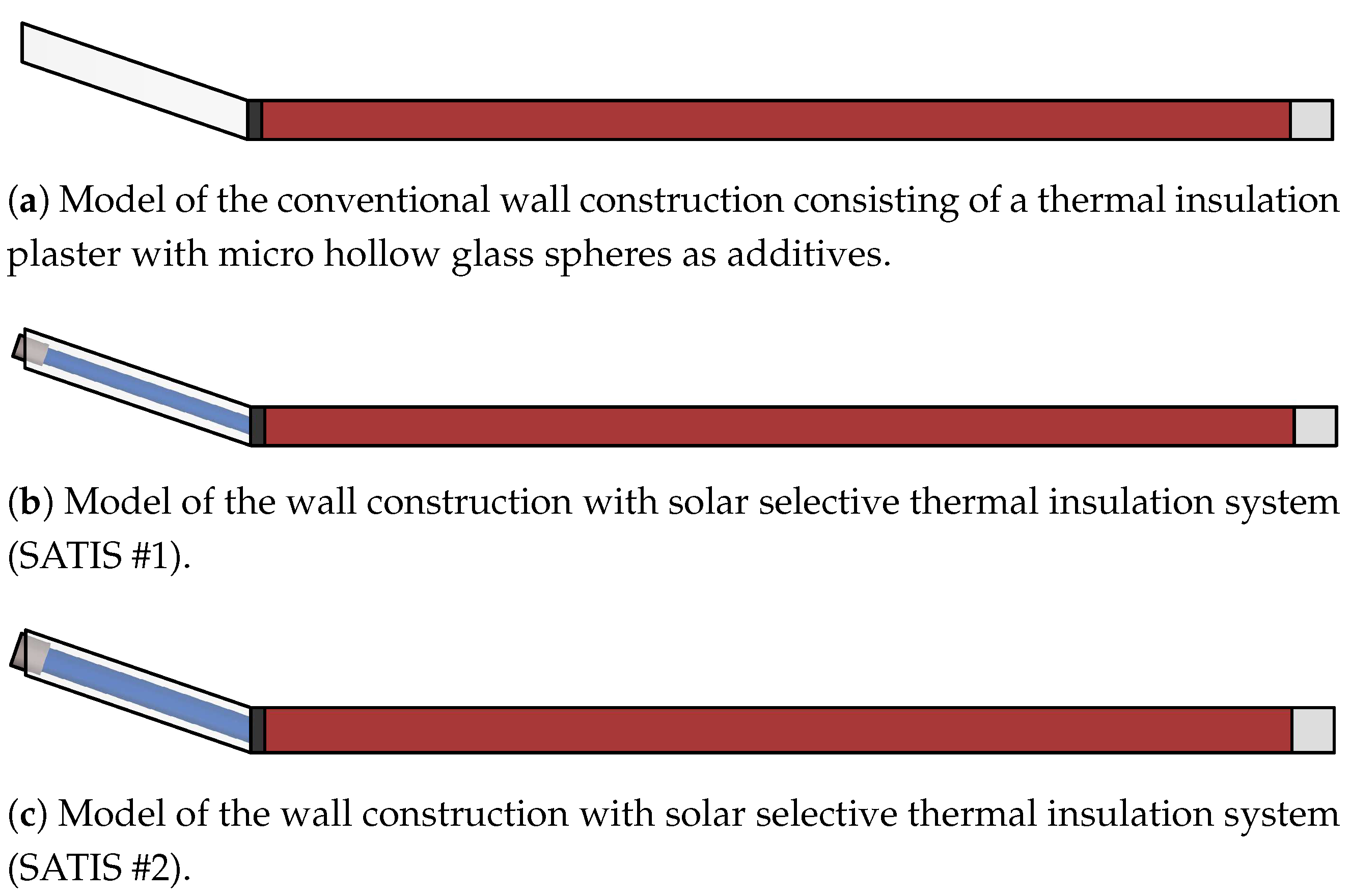
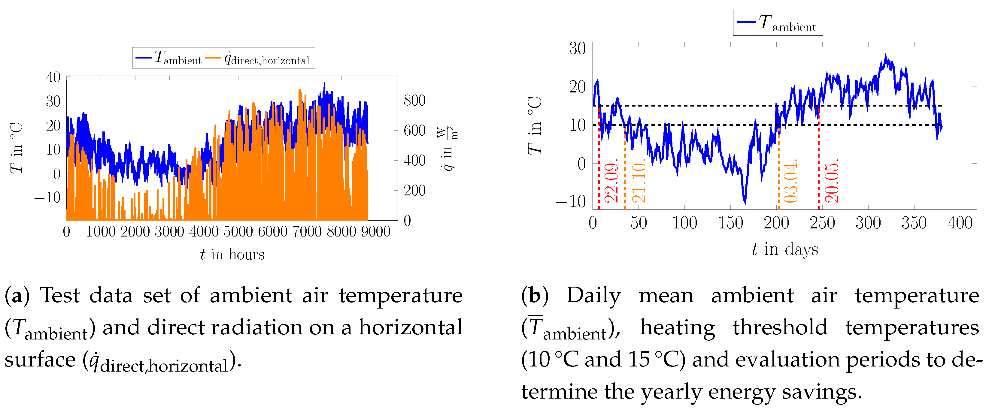
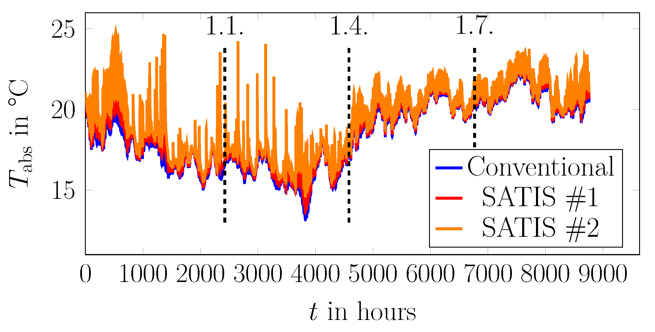
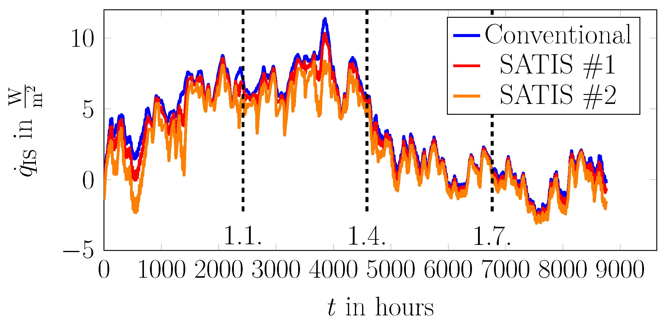
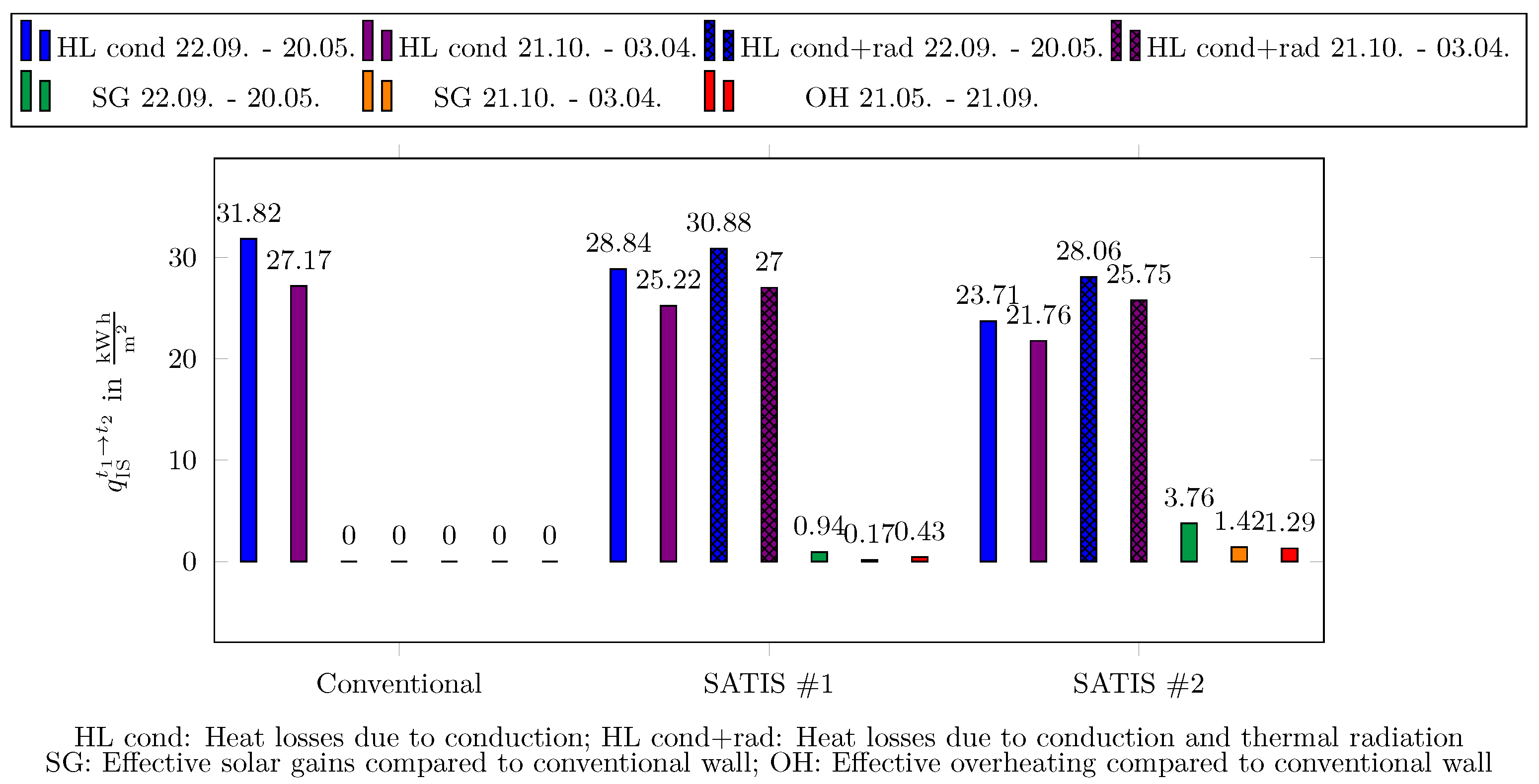
• In the yearly investigation, the variant SATIS #1, which deviates only slightly from the developed SATIS prototype (cf. Section 2.3), shows a reduced heat loss by 3% compared to the wall construction insulated with the same thermal insulation plaster, but without SATIS over the period from 22.09. to 20.05. (heating threshold temperature of 15 °C). Moreover, SATIS #2, which was optimized on the basis of the results of the parameter sensitivity analysis, shows a reduction in transmission heat losses of 11.8% over the same time period.
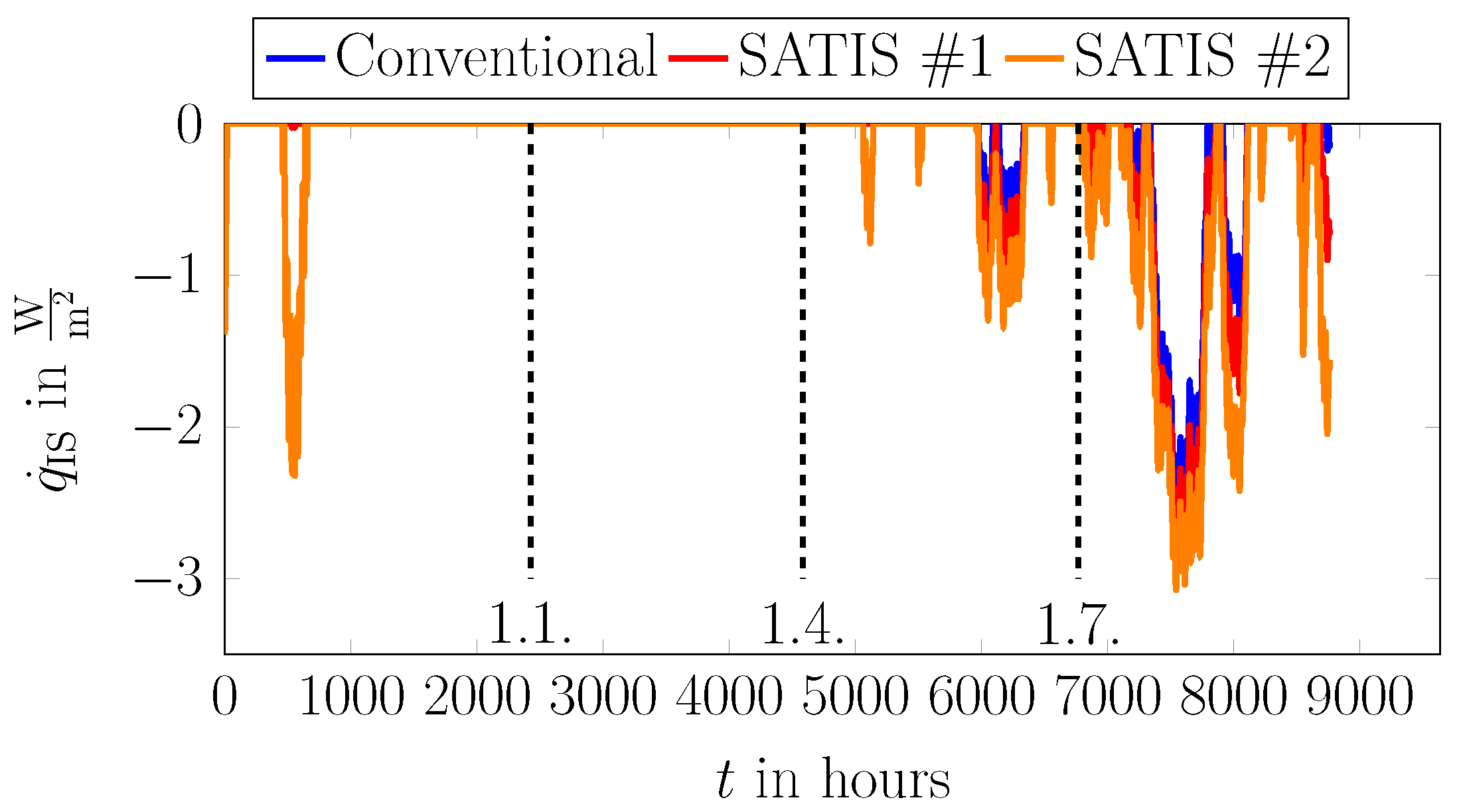
• If the heat gain released to the indoor space during the remaining period (21.05.–21.09.) is compared with the solar gains during the heating period (22.09.–20.05.), it can be observed that the absolute winter energy gain due to the modification of SATIS from #1 to #2 increases by 2.82 $\frac{\mathrm{k}\mathrm{W}\mathrm{h}}{{\mathrm{m}}^2}$, while the summer additional heat gain amounts to only 0.86 $\frac{\mathrm{k}\mathrm{W}\mathrm{h}}{{\mathrm{m}}^2}$.
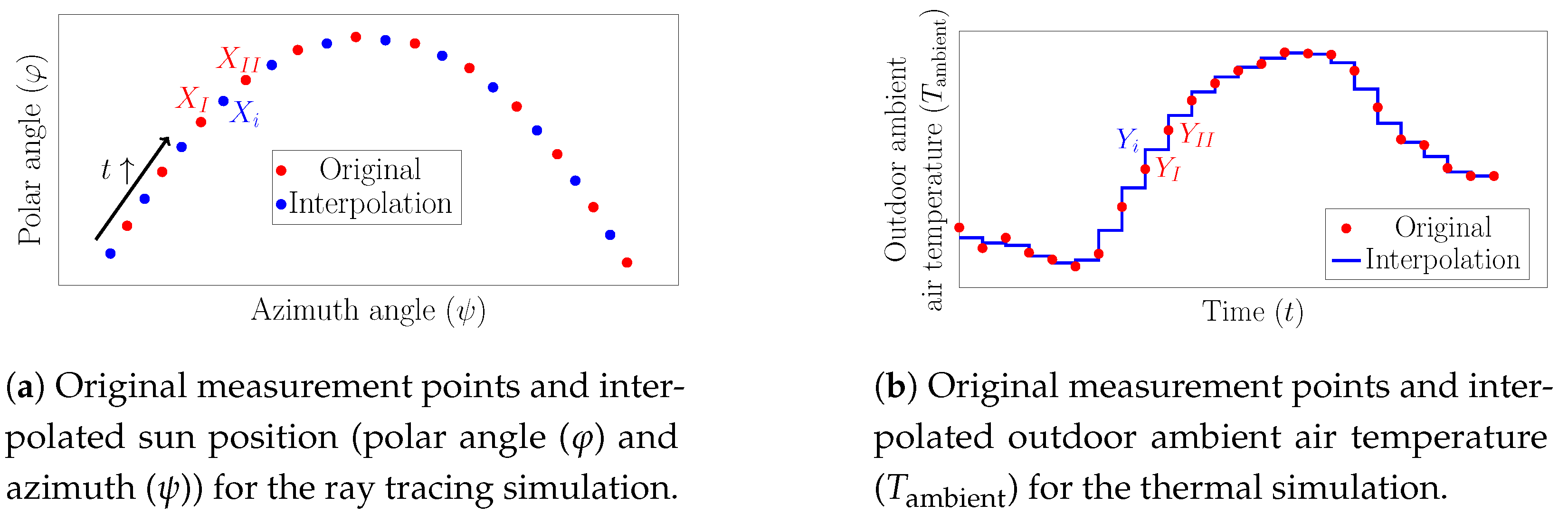
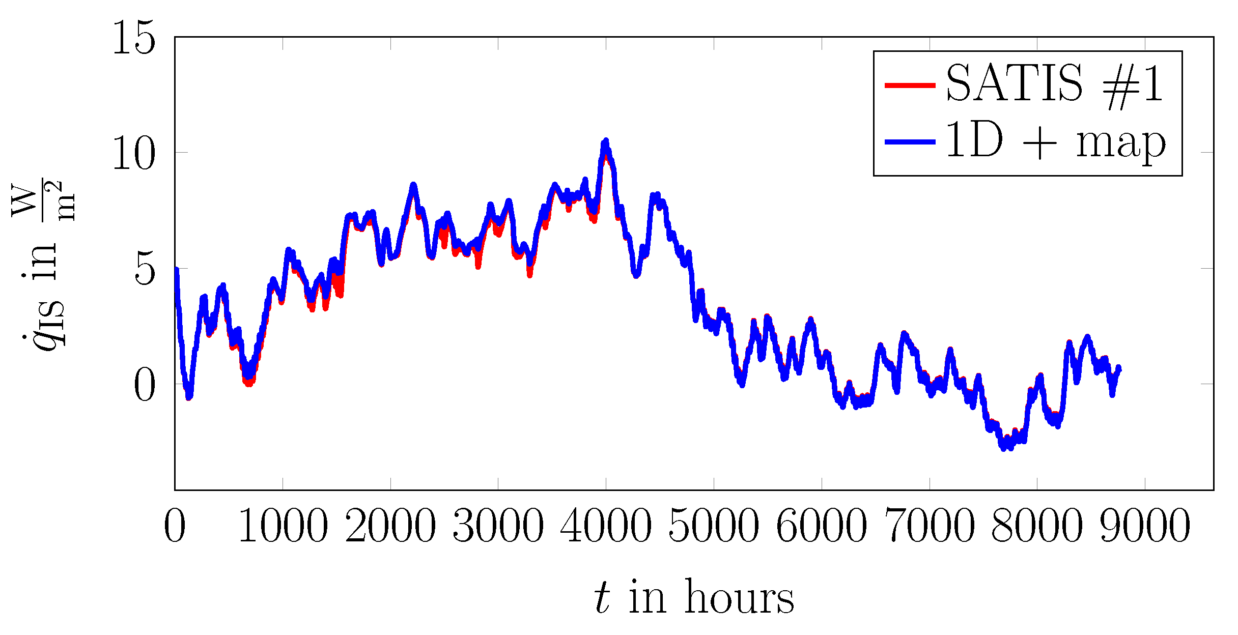
• The radiant heat flow map used for the 1D model was created with step sizes of the independent quantities of $\mathsf{\Delta }\phi =\mathsf{\Delta }\psi =2°$ and $\mathsf{\Delta }z=5 \mathrm{m}\mathrm{m}$ using ray tracing simulations at a reference intensity of 1000 $\frac{\mathrm{W}}{{\mathrm{m}}^2}$. Using SATIS #1, an integral yearly agreement of 98% of the 1D with the 3D model could be achieved with a reduction of the computation time from 312.5 h to 6.25 h.

References

1. Wong, I.L.; Eames, P.C.; Perera, R.S. A review of transparent insulation systems and the evaluation of payback period for building applications. Sol. Energy 2007, 81, 1058–1071. [Google Scholar] [CrossRef]
2. Kaushika, N.D.; Sumathy, K. Solar transparent insulation materials: A review. Renew. Sustain. Energy Rev. 2003, 7, 317–351. [Google Scholar] [CrossRef]
3. Paneri, A.; Wong, I.L.; Burek, S. Transparent insulation materials: An overview on past, present and future developments. Sol. Energy 2019, 184, 59–83. [Google Scholar] [CrossRef] [Green Version]
4. Russ, C. Einsatz transparenter Wärmedämmung zur Gebäudesanierung. In Energie; Hoffmann, V.U., Thiele, R., Eds.; Vieweg+Teubner Verlag: Wiesbaden, Germany, 1994; Volume 3, pp. 82–94. [Google Scholar] [CrossRef]
5. Symons, J.G. The Solar Transmittance of Some Convection Suppression Devices for Solar Energy Applications: An Experimental Study. J. Sol. Energy Eng. 1982, 104, 251–256. [Google Scholar] [CrossRef]
6. Platzer, W.J. Directional-hemispherical solar transmittance data for plastic honeycomb-type structures. Sol. Energy 1992, 49, 359–369. [Google Scholar] [CrossRef]
7. Platzer, W.J. Total heat transport data for plastic honeycomb-type structures. Sol. Energy 1992, 49, 351–358. [Google Scholar] [CrossRef]
8. Hollands, K.; Raithby, G.D.; Russell, F.B.; Wilkinson, R.G. Coupled radiative and conductive heat transfer across honeycomb panels and through single cells. Int. J. Heat Mass Transf. 1984, 27, 2119–2131. [Google Scholar] [CrossRef]
9. Schweiger, H.; Oliva, A.; Costa, M.; Perez Segarra, C.D. A Monte Carlo method for the simulation of transient radiation heat transfer: Application to compound honeycomb transparent insulation. Numer. Heat Transf. Part B Fundam. 1999, 35, 113–136. [Google Scholar] [CrossRef]
10. Kessentini, H.; Capdevila, R.; Castro, J.; Oliva, A.; Bouden, C. Three dimensional heat transfer analysis of combined conduction and radiation in honeycomb transparent insulation. Sol. Energy 2014, 105, 58–70. [Google Scholar] [CrossRef]
11. Platzer, W.J. The ALTSET Project: Measurement of angular properties for complex glazings. In Proceedings of the EuroSun 2000, ISES Europe Solar Congress, Copenhagen, Denmark, 19–22 June 2000. [Google Scholar]
12. Platzer, W.J. Energy performance assessment method: A step towards standardisation. In Proceedings of the EuroSun 98, the Second ISES Europe Solar Congress, Portoroz, Slovenia, 14–17 September 1998; Goetzberger, A., Ed.; Franklin: Birmingham, UK, 1999. [Google Scholar]
13. DIN Deutsches Institut für Normung e.V. Wärmeschutz und Energie-Einsparung in Gebäuden—Teil 6: Berechnung des Jahresheizwärme- und des Jahresheizenergiebedarfs. 2003. Available online: https://www.beuth.de/de/vornorm/din-v-4108-6/63939447 (accessed on 4 June 2021).
14. Platzer, W.J. Bestimmung des Solaren Energiegewinns Durch Massivwände Mit Transparenter Wärmedämmung; Richtlinie des Fachverbandes Transparente Wärmedämmung e.V.: Gundelfingen, Germany, 2000. [Google Scholar]
15. Liang Wong, I.; Eames, P.; Perera, S. Energy simulations of a transparent insulated office facade retrofit in London, UK. Smart Sustain. Built Environ. 2012, 1, 253–276. [Google Scholar] [CrossRef] [Green Version]
16. Świrska-Perkowska, J.; Kucharczyk, A.; Wyrwał, J. Energy Efficiency of a Solar Wall with Transparent Insulation in Polish Climatic Conditions. Energies 2020, 13, 859. [Google Scholar] [CrossRef] [Green Version]
17. Steininger, P.; Gaderer, M.; Steffens, O.; Dawoud, B. Experimental and Numerical Study on the Heat Transfer Characteristics of a Newly-Developed Solar Active Thermal Insulation System. Buildings 2021, 11, 123. [Google Scholar] [CrossRef]
18. Manz, H.; Egolf, P.; Suter, P.; Goetzberger, A. TIM–PCM external wall system for solar space heating and daylighting. Sol. Energy 1997, 61, 369–379. [Google Scholar] [CrossRef]
19. Steininger, P.; Gaderer, M.; Dawoud, B. Transient performance of a solar selective thermal insulation system. In Proceedings of the 16th Conference on Advanced Building Skins, Bern, Switzerland, 21–22 October 2021; Advanced Building Skins GmbH: Lucerne, Switzerland, 2021. [Google Scholar]
20. Steininger, P.; Gaderer, M.; Dawoud, B. Experimental and numerical study on the solar gain and heat loss of typical existing and refurbished German buildings. iCRBE Procedia 2020, 1, 75–93. [Google Scholar] [CrossRef]
21. Franken Maxit GmbH. maxit eco 72. 2020. Available online: https://docs.maxit.de:8443/procat/assets/images/TM-DE-GEECO72.pdf (accessed on 4 June 2021).
22. Lehmann, S.; Schwinger, L.; Scharfe, B.; Gerdes, T.; Ehrhardt, M.; Riechert, C.; Fischer, H.B.; Schmidt-Rodenkirchen, A.; Scharfe, F.; Wolff, F. Mikro-Hohlglaskugeln als Basis energieeffizienter Dämmung von Gebäuden. In Beiträge der Konferenz für neue Materialien im Bauwesen am 31. Januar 2018 in Berlin; Deutscher Ausschuss für Stahlbeton e.V., Ed.; Fraunhofer IRB Verlag: Berlin, Germany, 2018; pp. 21–25. [Google Scholar]
23. Schott, A.G. DURAN®: Tubing, Rods and Capillaries Made of Borosilicate Glass 3.3. 2016. Available online: https://www.schott.com/d/tubing/66ee849c-cad9-42a3-97cb-67fd0534e3fb/schott_duran_brochure_gb_final.pdf (accessed on 4 June 2021).
24. Kalkwerk Rygol GmbH & Co.KG. RYGOL Kalk-Gips-Leichtputz. 2018. Available online: http://www.rygol-sakret.de/fileadmin/user_upload/tm/tm_kalkgips_leichtputz_mip02_l.pdf (accessed on 4 June 2021).
25. Franken Maxit GmbH. Maxit Mur 900 Dünnbettmörtel. 2017. Available online: https://docs.maxit.de:8443/procat/assets/images/TM-DE-T1MUR%20900.pdf (accessed on 4 June 2021).
26. Kremer Pigmente GmbH & Co. KG. Iron Oxide Black 318, High Tinting. 2018. Available online: https://www.kremer-pigmente.com/media/pdf/48400_SDS.pdf (accessed on 4 June 2021).
27. DIN Deutsches Institut für Normung e.V. Bauteile—Wärmedurchlasswiderstand und Wärmedurchgangskoeffizient— Berechnungsverfahren. 2018. Available online: https://www.beuth.de/de/norm/din-en-iso-6946/255315365 (accessed on 4 June 2021).
28. Deutscher Wetterdienst. Stündliche Klimadaten. 2018. Available online: https://www.dwd.de/DE/leistungen/klimadatendeutschland/beschreibung_stundenwerte.html (accessed on 4 June 2021).
29. Schild, K.; Willems, W.M. (Eds.) Wärmeschutz; Springer Fachmedien Wiesbaden: Wiesbaden, Germany, 2013. [Google Scholar] [CrossRef]
30. Abdul Hamid, A.; Wallentén, P. Hygrothermal assessment of internally added thermal insulation on external brick walls in Swedish multifamily buildings. Build. Environ. 2017, 123, 351–362. [Google Scholar] [CrossRef]
31. Cascione, V.; Marra, E.; Zirkelbach, D.; Liuzzi, S.; Stefanizzi, P. Hygrothermal analysis of technical solutions for insulating the opaque building envelope. Energy Procedia 2017, 126, 203–210. [Google Scholar] [CrossRef]
32. Nageler, P.; Schweiger, G.; Pichler, M.; Brandl, D.; Mach, T.; Heimrath, R.; Schranzhofer, H.; Hochenauer, C. Validation of dynamic building energy simulation tools based on a real test-box with thermally activated building systems (TABS). Energy Build. 2018, 168, 42–55. [Google Scholar] [CrossRef]
Figure 1. Reference model of the solar selective thermal insulation system (SATIS).
Sustainability 13 07336 g001
Figure 2. Variation of the length and shape of the closure element.
Sustainability 13 07336 g002
Figure 3. Variation of the diameters and the area share on the outside surface of the wall of the light conducting element.
Sustainability 13 07336 g003
Figure 4. Simulation models for the investigation of the yearly energy saving potential.
Sustainability 13 07336 g004
Figure 5. Test data set, daily mean temperature and evaluation period to determine the energy savings of the solar selective thermal insulation system.
Sustainability 13 07336 g005
Figure 6. Interpolation procedure for solar position and outdoor air temperature in the yearly simulations.
Sustainability 13 07336 g006
Figure 7. Schematic representation of the one-dimensional modeling of the radiation distribution in the light conducting element of SATIS #1 via a heat source ( Q ˙ V φ t , ψ t , z , I S , t ).
Sustainability 13 07336 g007
Figure 8. Influence of various construction parameters on the effective thermal conductivity ( λ eff ).
Sustainability 13 07336 g008
Figure 9. Influence of different construction parameters on the total solar energy transmittance (g).
Sustainability 13 07336 g009
Figure 10. Temperature in the absorber or behind the insulation layer ( T abs ) for the solar selective wall constructions (#1 and #2) and the wall construction insulated with the same thermal insulation plaster but without SATIS (“Conventional”).
Sustainability 13 07336 g010
Figure 11. Heat flux on the inside surface of the wall ( q ˙ IS ) for the solar selective wall constructions (#1 and #2) and the wall construction insulated with the same thermal insulation plaster but without SATIS (“Conventional”).
Sustainability 13 07336 g011
Figure 12. Heat flux released into the indoor space ( q ˙ IS < 0 W m 2 ) for the solar selective wall constructions (#1 and #2) and the wall construction insulated with the same thermal insulation plaster but without SATIS (“Conventional”).
Sustainability 13 07336 g012
Figure 13. Heat losses due to conduction (HL cond), heat losses due to conduction and thermal radiation (HL cond+rad), effective solar gains (SG) and effective overheating (OH) of the solar selective wall constructions (#1 and #2) compared with the wall construction insulated with the same thermal insulation plaster, but without SATIS (“Conventional”) for different evaluation periods.
Sustainability 13 07336 g013
Figure 14. Radiant heat flow map of the solar selective wall construction #1 (symmetric about φ -axis, computed for Δ φ = Δ ψ = 2 ° and Δ z = 5   m m ).
Sustainability 13 07336 g014
Figure 15. Comparison between the heat flux on the inside surface of the wall ( q ˙ IS ) of the solar selective wall construction #1 and the one-dimensional model using the computed radiant heat flow map.
Sustainability 13 07336 g015