
Perceived Trip Time Reliability and Its Cost in a Rail Transit Network


1
School of Transportation and Logistics, Southwest Jiaotong University, Chengdu 610031, China
2
Faculty of Transportation Engineering, Kunming University of Science and Technology, Kunming 650093, China
3
A. James Clark School of Engineering, University of Maryland, College Park, MD 20740, USA
*
Author to whom correspondence should be addressed.
Sustainability 2021, 13(13), 7504; https://0-doi-org.brum.beds.ac.uk/10.3390/su13137504
Submission received: 15 May 2021
/
Revised: 11 June 2021
/
Accepted: 22 June 2021
/
Published: 5 July 2021
(This article belongs to the Topic Industrial Engineering and Management)
Abstract
:Time reliability in a Rail Transit Network (RTN) is usually measured according to clock-based trip time, while the travel conditions such as travel comfort and convenience cannot be reflected by clock-based trip time. Here, the crowding level of trains, seat availability, and transfer times are considered to compute passengers’ Perceived Trip Time (PTT). Compared with the average PTT, the extra PTT needed for arriving reliably, which equals the 95th percentile PTT minus the average PTT, is converted into the monetary cost for estimating Perceived Time Reliability Cost (PTRC). The ratio of extra PTT needed for arriving reliably to the average PTT referring to the buffer time index is proposed to measure Perceived Time Reliability (PTR). To overcome the difficulty of obtaining passengers’ PTT who travel among rail transit modes, a Monte Carlo simulation is applied to generated passengers’ PTT for computing PTR and PTRC. A case study of Chengdu’s RTN shows that the proposed metrics and method measure the PTR and PTRC in an RTN effectively. PTTR, PTRC, and influential factors have significant linear relations among them, and the obtained linear regression models among them can guide passengers to travel reliably.
1. Introduction
As travel demand increases, passengers in large cities experience increasing congestion, crowding, and low time reliability. Time reliability not only reflects the service quality of transportation networks, but also affects passengers’ route choices [1] and travel satisfaction [2]. Passengers who require high time reliability, such as commuters, are willing to pay for such reliability [3]. Both transportation managers and passengers consider time reliability to be very important.
Many studies have explored time reliability for road networks [4,5], Rail Transit Networks (RTNs) [6,7], and bus networks [8,9]. Although these studies have proposed measures for evaluating the time reliability of transportation networks, travel conditions such as the number of transfer times, crowding, and seat availability in vehicles that affect passengers’ perceptions have been relatively neglected [10]. The reason is that time reliability is measured based on clock-based trip time, which neglects travel conditions. Let us assume that passengers A and B travel between the same Origin to Destination Station (OD) pair and spend the same time to arrive at the destination station. However, if passenger A gets a seat in an uncrowded vehicle while passenger B stands in a crowded vehicle, their travel conditions vary greatly despite having the same time reliability. Therefore, both clock-based trip time and the passengers’ travel conditions are incorporated here to measure the Perceived Time Reliability (PTR) and Perceived Time Reliability Cost (PTRC). The extra PTT needed for arriving reliably equaling the difference between the 95th percentile PTT and average PTT, is converted into the monetary cost for estimating PTRC. Referring to the buffer time index, the ratio of extra PTT needed for arriving reliably to the average PTT is proposed to measure PTR. To reveal the relations among PTR and influential factors, as well as the relations among PTRC and influential factors, multiple linear regression models were developed and determined by applying the stepwise regression method [11].
The remainder of this paper is organized as follows: the literature review discusses the previous research on time reliability. In the methodology section, the probability distributions of trip time components are introduced, the metrics of PTR and PTRC are proposed, multiple linear regression models are developed among PTR and influential factors, as well as among PTRC and influential factors, after which the PTR and PTRC estimation procedure are introduced. The PTR and PTRC for Chengdu’s RTN are estimated in the case study. The results of applying the stepwise regression method for obtaining the linear regression models are analyzed. Finally, the conclusions of the study are summarized.
2. Literature Review
The concept of time reliability was commonly associated with the variability of time [12]. Researchers studied time reliability from the perspectives of operators [13], travelers [14], and planners [15] in recent years. To measure the time reliability of transportation networks from the perspective of operations, some indicators such as punctuality of transportation schedule indicator, on-time classification, coefficient of headways’ variation, and weighted delay indicators [16,17] were proposed. Although those indicators could measure the stability of transportation schedules and differences in the passengers’ waiting times, they could not guide the travelers’ decisions directly, nor did they analyze the time reliability in terms of the travelers’ total trip time.
It has become much easier to obtain travelers’ trip times from Automatic Fare Collection (AFC) data, Global Positioning Systems (GPS) data, and Automatic Vehicle Location (AVL) data. Therefore, researchers analyzed the time reliability for transportation networks with these data [17]. The distribution of time in a road network was estimated according to GPS data [18]. The time reliability of Chengdu’s urban rail transit network was measured by using AFC data [7]. The AVL data were used to estimate path travel time variance according to travel time variances on paths’ segments [19]. The AFC data were effective for obtaining travelers’ trip time and analyzing time reliability for urban rail transit networks or bus networks. However, these data could not be used to obtain travelers’ trip time for different transportation modes. Thus, if a person took a train with one ticket and then took a bus with another ticket, the trip time could not be fully determined from AFC data since the identification numbers of the two tickets differed. It was a common phenomenon that passengers used different tickets to travel on China’s RTNs since different companies managed different modes of rail transit (such as urban rail transit, high-speed railway, and suburban railway) and issued different kinds of tickets.
Various metrics were proposed to measure the time reliability of transportation networks, as shown in Table 1. The buffer time index was widely used for measuring time reliability in transportation networks since it not only measured the time reliability but also guided passengers to allow additional time for reliably reaching their destinations. Thus, the time reliability of London’s Underground was evaluated with the buffer time index according to the passengers’ trip time obtained from AFC data [20]. The buffer time index for London bus routes was evaluated using AVL data [21]. The design criteria for the time reliability metric from the passengers’ perspective were proposed by [22], who noted that the buffer time index satisfied the criteria for measuring time reliability.
The methods found for measuring time reliability may be categorized into three groups: analytical approaches, statistical approximation, and simulation approaches. The analytical approaches can be applied under different traffic conditions. However, their main drawback is the high complexity of their estimation process for time distributions at the network level [29]. The Normal, Lognormal, Gamma, Truncated Normal/Lognormal, and Weibull distributions have been applied to compute time reliability using statistical methods [23,30]. The mixture of distribution models was used to measure time reliability since the single distribution model could not well represent the time distribution. However, it was difficult to determine the mix of distribution models. For simulation approaches, the time reliability of a transportation network could be estimated in different scenarios (extreme weather, transportation accidents, and transportation control). The simulation approaches can also be applied to measure the time reliability when demand and capacity fluctuate [31,32]. A simulation approach may be applied very flexibly, but at high computation cost, to measure the time reliability of transportation networks.
The literature review shows that researchers emphasized measuring time reliability in terms of variability of clock-based trip time. However, the passengers’ travel conditions are neglected when measuring the time reliability of transportation networks. Here, passengers’ Perceived Trip Time (PTT), which integrates travel conditions (i.e., the number of transfer times, crowding, and seat availability in the vehicle), and the clock-based trip time are computed and used for measuring the PTR and PTRC in an RTN. It is difficult to apply analytical approaches and statistical approximation to measure the PTR for the RTN because the passengers’ trip components are complex and the distributions of trip time components are different. In addition, passengers may use different tickets to travel on different rail transit modes, which complicates matching the ticket numbers to obtain the passengers’ trip times. Therefore, a Monte Carlo simulation is used here to generate passengers’ PTT for measuring PTR and PTRC in an RTN. The simulation process for a large network only lasts a few minutes due to advances in computing power and speed.
3. Methodology
In this section, the computation of the passengers’ PTT and the probability distributions of clock-based trip time components are introduced. After that, the metrics for measuring PTR and PTRC on paths, among OD pairs, on lines, and an RTN are proposed. Then, the method for estimating PTR and PTRC based on passenger trip assignment and Monte Carlo simulation is proposed.
3.1. Passenger’s Clock-Based Trip Time and PTT
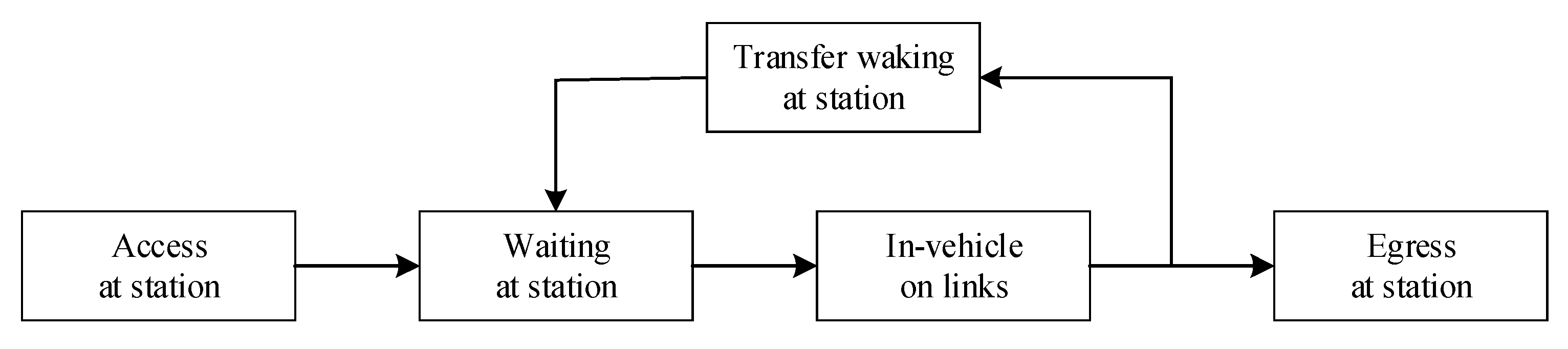
The clock-based trip time on a path between an OD pair includes access, egress and transfer walking time, waiting time at the origin and transfer stations as well as in-vehicle time. The clock-based trip time components are shown in Figure 1. The clock-based trip time is different from the passengers’ PTT. Studies show that the components of clock-based trip time are perceived differently by passengers, e.g., waiting time has a much higher perceived value than in-vehicle time in uncrowded vehicles. The number of transfer times, crowding in vehicles, and reduced seat availability also increase the passengers’ PTT [33].
The crowding level and seat availability in trains, as well as the number of transfer times affect passengers’ PTT [34]. Therefore, the weighted in-vehicle time is computed according to crowding level and seat availability in trains. The transfer penalty time is computed according to transfer time and the number of transfer times. , which is estimated with Equation (1), is the PTT for passenger n traveling from station to station on path :
where , , and are walking time at station , walking time at station and waiting time at station , respectively, for passenger traveling from station to station on path . is in-vehicle time on link . is the set of links from station to station on path . and , are walking time and waiting time, respectively, for passenger traveling on path . is the set of transfer stations from station to station on path . is the number of transfer times The time weights and are used here according to [35]. The values of and stay the same when computing the PTTs for different paths. The time weight is related to crowding in trains and seat availability on link . The load factor, which is the ratio of passengers to seats on a vehicle, is used to reflect the train crowding. The values of at different load factors when passengers sit or stand are shown in Table 2 according to [36].
3.2. Probability Distributions of Clock-Based Trip Time Components
The values of trip time vary since clock-based trip time components are random variables subject to probability distributions. The probability distributions of clock-based trip time components are obtained and used in Monte Carlo simulation [37] to generate the passengers’ PTT.
3.2.1. Probability Distributions of Walking Time
The passengers’ walking time at stations is affected by many factors, such as the degree of congestion, accessibility of facilities, and the passengers’ age and genders. Here, only two essential factors, i.e., walking distance (considers walking distances on the passageways, upstairs, and downstairs) and walking speed are considered when determining the walking time distribution. The walking speed follows an distribution on passageways, upstairs, and downstairs. The values of and are shown in Table 3 according to [38].
The walking time is the sum of the ratios of walking distance to walking speeds, and thus the walking time distributions on passageways , upstairs and downstairs in path are calculated following Equations (2)–(4):
where , and are walking distances on passageways, upstairs, and downstairs, respectively.
3.2.2. Probability Distributions of Waiting Time
The waiting time distributions on frequency-based lines and schedule-based lines vary greatly because passengers can use their tickets for any trains on frequency-based lines but only for a specific train on schedule-based lines. When passengers wait on a frequency-based line, they may have an extra waiting time if some trains have insufficient capacity. When passengers wait on a schedule-based line, they can board their intended trains as long as they have tickets for those trains since the tickets are sold according to the trains’ capacities.
- (1)
- Probability Distribution of Waiting Time on Frequency-based Lines
The passengers’ arrivals at stations on frequency-based lines such as metro lines are Poisson-distributed [38]. Passengers waiting at frequency-based lines have normal waiting time and extra waiting time. The normal waiting time means that passengers can board the first arriving train. The normal waiting time is a uniformly distributed random variable ranging from 0 to the headways on lines [39] as shown in Equation (5):
where and are the passengers’ normal waiting times at station and the headway of a line that includes . is the set of stations that are on frequency-based lines.
Passengers may have extra waiting times due to the first arriving train not having enough capacity for all waiting passengers. One successful boarding at station requires independent trials, each with a probability of success [40]. In addition to the first arriving train, the probability that passengers need to wait longer for arriving trains on the platform represented as is estimated with Equation (6).
is the probability that passengers board a train successfully at station . is related to the passenger flow and remaining capacity of a link in the direction of intended boarding trains and connected with directly, which is estimated with Equation (7):
where and are the capacity and passenger flow on link which is in the direction of intended boarding trains and connected with directly.
According to Equation (6), the number of subsequent trains that passengers must wait for is geometrically distributed [40]. Thus, the extra waiting time at station that equals the headway multiplied by the number of subsequent passing trains has the following distribution (Equation (8)):
- (2)
- Probability Distribution of Waiting Time on Schedule-based Lines
To avoid missing their intended boarding trains, passengers arrive at the stations in advance. Passengers waiting on schedule-based lines have no extra waiting time since the tickets are sold according to the trains’ capacities. The probability density function of waiting time on schedule-based operation lines (such as high-speed railway lines) follows the mixed distribution of beta and gamma distributions as Equation (9) according to [41]:
where are the waiting times at station . is the station set on schedule-based lines. and represent the fractions of the beta distribution and gamma distribution, respectively. , and are gamma distributions.
3.2.3. Probability Distribution of In-Vehicle Time
The trains’ running time on a link is normally distributed, and the expected running time is proportional to the standard deviation, according to [40]. Therefore, the in-vehicle times on a link are normally distributed as Equation (10):
where is the expected in-vehicle time on link , which can be estimated with the mean of train running time on link . is 0.04 according to [40]. is the set of links in an RTN.
3.3. PTR and PTRC Metrics
3.3.1. PTR and PTRC on a Path
The extra PTT needed for arriving reliably equals the 95th percentile PTT minus the average PTT, computed with Equation (11). The ratio of the extra PTT needed for arriving reliably to average PTT is used for measuring PTR and is computed with Equation (12):
where , and are the extra PTTs needed for arriving reliably, 95th percentile PTT, and average PTT, respectively, from station to station on path , . is the set of stations in an RTN. is PTR from station to station on path .
The extra PTT needed for arriving reliably is converted to a monetary cost according to Equation (13) to estimate PTRC.
where is the PTRC from station to station on path . is the value of the time parameter that converts PBT into a monetary cost, which is related to the passengers’ income [34].
3.3.2. PTR and PTRC among OD Pairs
The PTR and PTRC between an OD pair equal the average PTR and average PTRC for passengers who travel between that OD pair. PTR and PTRC from station to station ( and ) are estimated with Equations (14) and (15), respectively:
where is the total number of travel paths selected by passengers from station to station . and are passenger trips from station to station on path and from station to station , respectively.
In Equations (15) and (16), , thus can be estimated by computing the probability of path being selected by passengers when they travel from station to station . The probabilities of paths selected by passengers can be determined after passenger trip assignments.
3.3.3. PTR and PTRC on Lines
The PTR computed with Equation (16) and PTRC computed with Equation (17) on a line equal the respective average PTR and average PTRC for passengers whose origin station or destination station is on that line.
where is the set of lines in an RTN. is the station set on line . and are passenger trips from station to station and from station to station , respectively.
3.3.4. PTR and PTRC in an RTN
The average PTR for all passengers computed with Equation (18) is used to estimate PTR on the RTN:
where is the PTR of the RTN and is passenger trips on the RTN.
The PTRC in an RTN C computed with Equation (19) is estimated with the average PTRC for all passengers:
3.4. PTR and PTRC Estimation Based on Passenger Trip Assignment and Monte Carlo Simulation
To measure PTR and PTRC in an RTN, passenger trips are assigned to the RTN to determine load factors (which are shown in Table 2) and probabilities of paths being selected by passengers. Here, a length-based C-logit stochastic user equilibrium model is applied to assign passenger trips. The model is solved by the method of successive weighted averages [42]. Then, a Monte Carlo simulation [37] is applied to generate passengers’ PTT according to probability distributions of trip time components for computing PTR and PTRC on the RTN.
3.4.1. The Length-Based C-Logit Stochastic User Equilibrium Model
The length-based C-logit stochastic user equilibrium model is applied to assign passenger trips since it effectively reflects the overlapping effect among paths and the passengers’ travel characteristics [43]. The length-based C-logit Stochastic User Equilibrium model is shown in Equations (20)–(27):
subject to:
In the objective function, is a non-negative parameter. The higher the value of , the higher the accuracy of the passengers’ perception of paths’ trip time and the closer the assignment to the equilibrium assignment. is the PTT on link , which equals the in-vehicle time multiplied by its time weight (i.e., in Table 2). , which is the common factor for path is computed with constraint (21). It measures the similarities of path with other paths in the same OD pair according to length of common links. is the sum of common links’ lengths on paths and from station to station . and are lengths of paths and , respectively, from station to station . is a parameter in Equation (26). If then the length-based C-logit route choice model collapses to a Multinomial Logit model. If then the route choice probabilities in the limiting case of N coincident paths tend to 1/N of those computed with a Multinomial Logit model applied while considering the coincident paths as a single path [44]. is used here according to [45]. In constraint (22), equals the passenger trips traveling from station to station (i.e., ) multiplied the probability of path being selected by passengers (i.e., which is computed with constraint (23)). is the passenger flow on link , which is computed with constraint (24). is a binary variable, which is 0 if the path k from station to station contains link and 1 otherwise. Constraints (25) and (26) compute the hourly number of seats on link (i.e., ) and the capacity of link (i.e., ), respectively; they equal the frequency of trains passing through link (i.e., ) multiplied by the seats per train (i.e., and the capacity per train (i.e., . in constraint (27) is the load factor on link , which measures crowding levels in vehicles on that link.
3.4.2. The Method of Successive Weighted Averages
The Length-based C-logit Stochastic User Equilibrium model is solved with the method of successive weighted averages [42] to assign passenger trips on the RTN, as follows:
- Step 1:
- Set the iteration’s number , the algorithm variable , the algorithm parameter , and the stop iteration criterion . The effective path sets among OD pairs are determined using Yen’s algorithm. The PTTs of paths in the effective travel path sets are computed without considering passenger flow.
- Step 2:
- Passenger trips are assigned to the RTN with Equations (23) and (24) according to the PTTs of effective travel paths to compute passenger flow on each link, which is represented as .
- Step 3:
- The PTTs of effective travel paths among OD pairs are computed according to the passenger flows on links . The passenger trips among OD pairs are assigned to the RTN again. The passenger flow on each link, is recomputed.
- Step 4:
- Let , and . Passenger flows on links are updated with Equation (28):
- Step 5:
- Convergence assessment. If , then stop iterating and is the passenger flow after passenger trip assignment; otherwise, go to step 3.
The passenger flows on links and the probabilities of paths being selected by passengers are determined according to the above five steps. The load factor on a link is estimated as the ratio of hourly passenger flow on that link to the provided seats per hour on that link. Thus, the weight of in-vehicle time is determined from Table 2.
3.4.3. The Method of Successive Weighted Averages
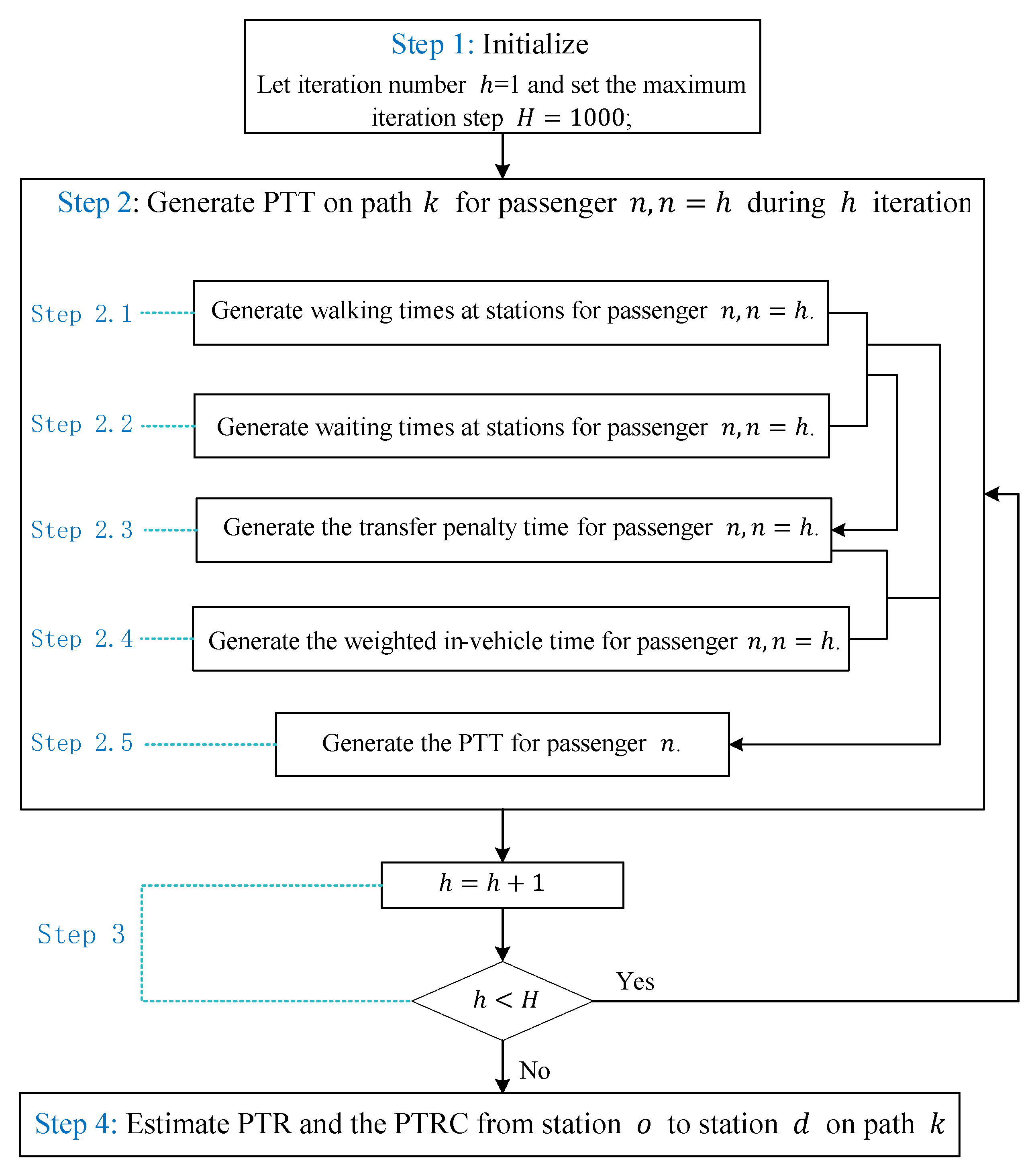
The PTR and PTRC are estimated by applying a Monte Carlo simulation after passenger trips are assigned to the RTN. According to the probability distributions of clock-based trip time components introduced in Section 3.2, the PTTs of passengers from station to station on path are generated by applying Monte Carlo simulation as follows:
Step 1: Initialize.
Initialize the iteration number = 1 and set the maximum iteration step ;
Step 2: Generate PTT on path for passenger during iteration.
Step 2.1: Generate walking times at stations for passenger .
The walking distances on passageways , upstairs and downstairs at origin station , destination station and transfer stations on path are determined and then passenger ’s walking times on passageways, upstairs, and downstairs at each station are generated with Equations (2)–(4) in Section 3.2.1. Thus, passenger ’s walking times at origin station , destination station and transfer stations represented as , and , respectively, are the sum of walking time on passageways, upstairs, and downstairs at station , station and transfer station .
Step 2.2: Generate waiting times at stations for passenger .
Passenger ’s waiting times at origin station and transfer stations on path represented as and respectively, are generated. To generate a waiting time at a station for passenger , the operation type of the line to which that the waiting station belongs is determined.
If the operation type is a frequency-based line, then the waiting time at the station is generated as follows: The normal waiting time at the station is generated according to Equation (5); The link that is in the direction of intended boarding trains and connected with the waiting station directly is determined. Then, the probability of successful boarding is estimated with Equation (7). After that, an extra waiting time at the waiting station is generated with Equation (8). The total generated waiting time is the sum of the generated normal waiting time and the generated extra waiting time.
If a waiting station belongs to a schedule-based line, then passengers waiting at that station do not have extra waiting time and the waiting time at that station is generated with Equation (9).
Step 2.3: Generate the transfer penalty time for passenger .
The equation is used to computed the generated transfer penalty time according to the generated walking time and waiting time at transfer stations in steps 2.1 and 2.2.
Step 2.4: Generate the weighted in-vehicle time for passenger .
The link set on path from station to station is determined. The weight of in-vehicle time for each link (i.e., ) is determined after passenger trips are assigned. Passenger ’s in-vehicle time on each link (i.e., ) is generated according to Equation (10). Finally, computes the generated weighted in-vehicle time for passenger on path .
Step 2.5: Generate a PTT for passenger .
Equation (1) computes the generated PTT for passenger traveling on path according to generated times in steps 2.1 to 2.4.
Step 3: Stop assessment.
Let = + 1. If , return to step 2; otherwise, go to step 4.
Step 4: Estimate PTR and the PTRC from station to station on path .
The passengers’ PTTs are generated according to steps 1 to 3. The 95th percentile PTT is the 950th PTT in the generated 1000 PTTs’ rank sorted from smallest to largest. The extra PTT needed for arriving reliably, represented as equals the 95th percentile PTT minus the average PTT. Thus, the PTR and the PTRC on path are estimated with Equations (12) and (13), respectively.
The steps for estimating PTR and PTRs from station to station on path are shown in Figure 2. Thus, PTR and PTRC among OD pairs, on lines as well as on the RTN are estimated with Equations (14)–(19).
4. Case Study
PTR and PTRC on Chengdu’s RTN are measured, and the regression relating PTRS and PTRC to influential factors is analyzed in this section. Some measures for enhancing PTR and reducing PTRC on Chengdu’s RTN are proposed based on the results.
4.1. Chengdu’s RTN
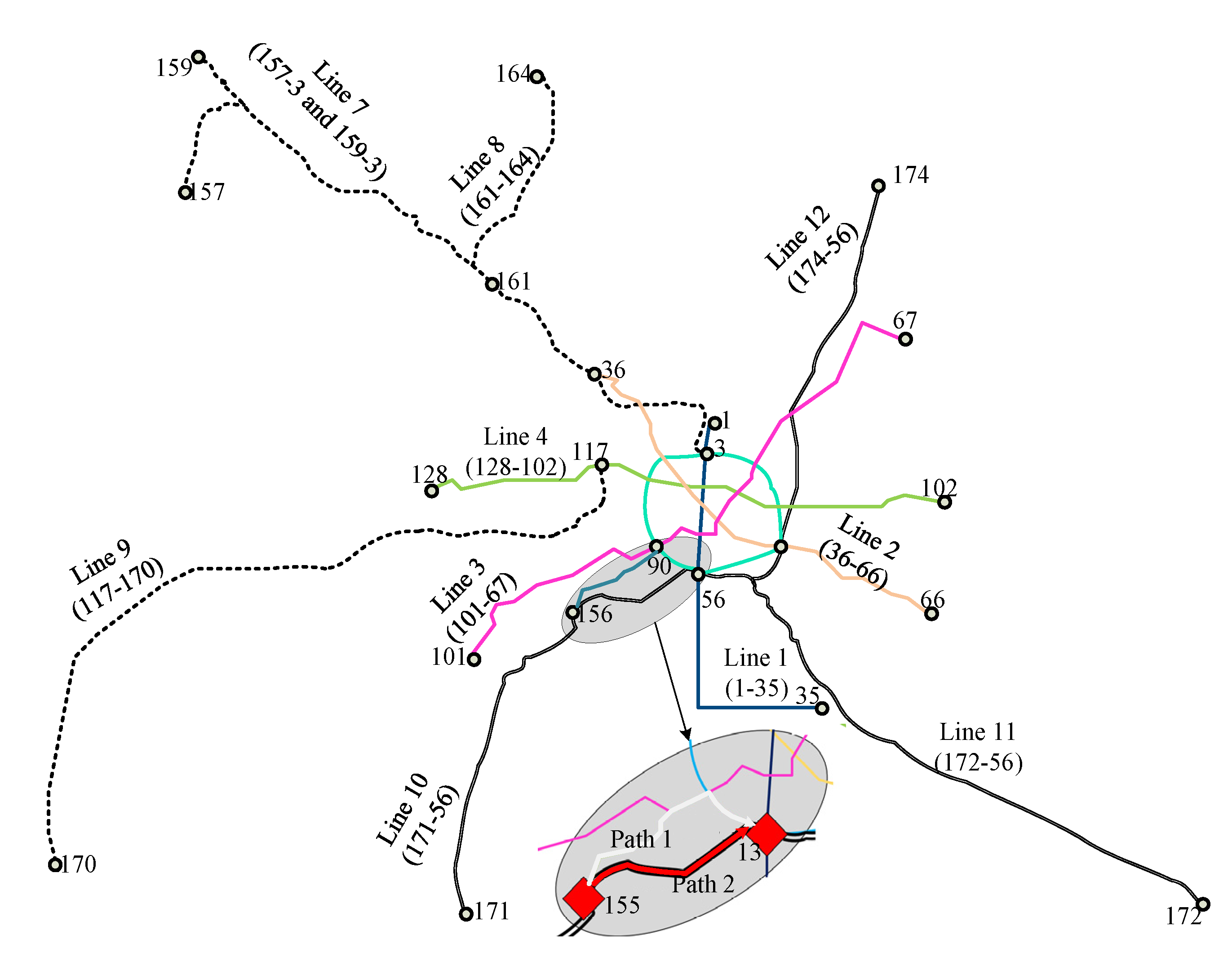
The transfer and terminal stations on lines, as well as the modes of lines in Chengdu’s RTN are shown in Figure 3a. There were six metro lines (lines 1 to 6), including three suburban railway lines (lines 7 to 9) and three high-speed rail lines (lines 10 to 12), as well as 174 stations on Chengdu’s RTN in May 2019. Some details of the metro network are shown in Figure 3b. The public transportation trips in urban and suburban areas, as well as between Chengdu and other nearby cities are mainly served by metro lines and suburban railway lines as well as high-speed rail lines.
4.2. Chengdu’s RTN Operation Data and Surveyed Data
The operation type, headways, capacity per hour, and provided seats per hour on Chengdu’s rail transit lines during morning peak periods (from 7:30 a.m. to 9:30 a.m.) are shown in Table 5.
With the support of the National Key R & D Program of China, our team conducted surveys on Chengdu’s RTN. The average walking distances on passways, upstairs, and downstairs for investigated stations are estimated to be nearly 300 m, 15 m, and 15 m, respectively. Those walking distances are used to generate walking time using Monto Carlo simulation when passengers access and egress stations since determining the walking distances on passways, upstairs, and downstairs for 174 stations in Chengdu’s RTN is difficult. The transfer walking distances on upstairs and downstairs are estimated to be 10 m. The transfer walking distances (sum of walking distances on passways, upstairs, and downstairs) at all transfer stations, train running times on all links, as well as the OD trip distribution in Chengdu’s RTN during morning peak periods, are obtained from an operator and a survey [7]. The passenger trips among OD pairs are shown in Figure 4. The arcs represent the number of passenger trips traveling among OD pairs during morning peak periods. Darker arcs represent higher passenger trips among OD pairs. To limit this paper’s length, line 1 is taken as an example to show transfer walking distances on line 1’s transfer stations and train running times on line 1’s links, which are listed in Table 6; Table 7, respectively.
The passenger trips among OD pairs are assigned to the network using the Length-based C-logit Stochastic User Equilibrium Model. The PTR and PTRC among OD pairs can be estimated with Monte Carlo simulation according to the above data. In estimating the PTRC, the value of time parameter equals 30% of household income per hour according to economist Kenneth Gwilliam’s recommendation [46]. The average household income is 134,187 ¥/per year which is obtained from the “Chengdu Statistical Yearbook-2018” [47]. The work time per week is 46 h according to the data released by the National Bureau of Statistics. There are nearly 52 weeks per year. Therefore, the work hours are 2392 h per year and thus the average household income per hour is 56.10 ¥/hour. The value of time parameter γ, which equals 30% of household income per hour, is 16.83 ¥/hour.
4.3. PTR and PTRC Estimation
4.3.1. PTR and PTRC among OD Pairs
The PTRs and PTRCs on two paths from station 155 to station 13, which are shown in Figure 5, are estimated. This is shown as an example of measuring PTR and PTRC on paths.
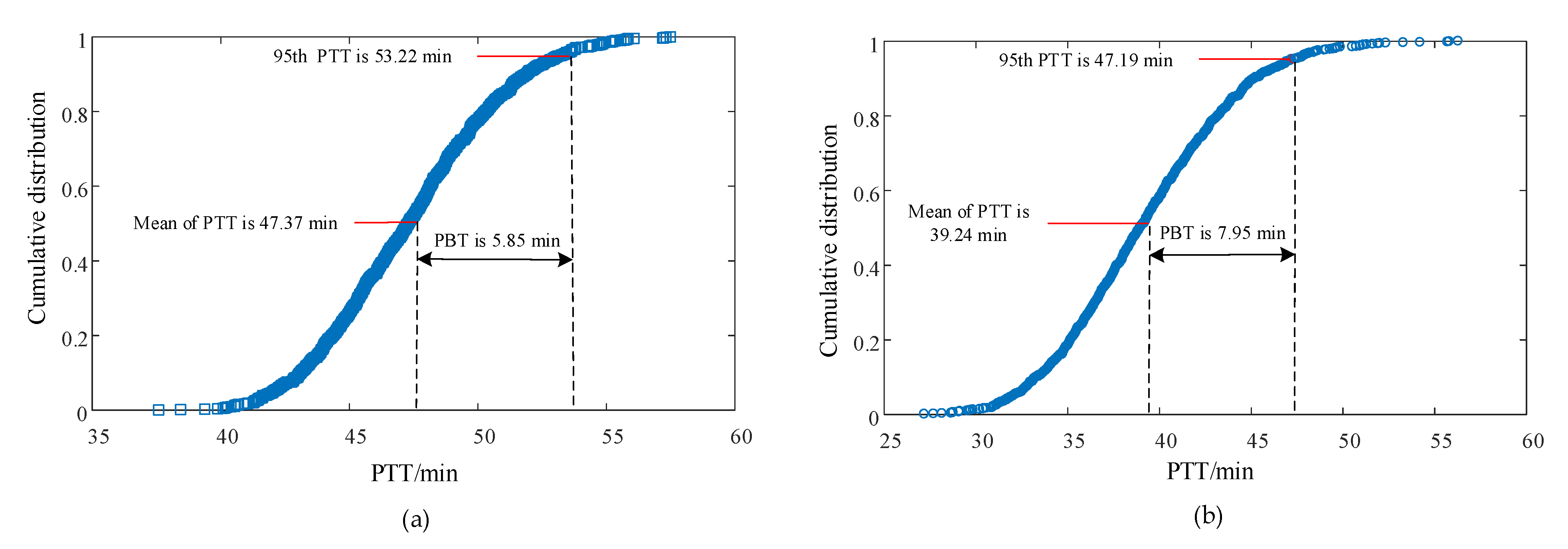
The cumulative distributions of generated 1000 passengers’ PTTs on paths 1 and 2 using Monte Carlo simulation are shown in Figure 6a,b, respectively. The PTRs on paths 1 and 2 are estimated to be 0.135 and 0.203, respectively, according to the mean PTT and 95th percentile PTT on paths 1 and 2. The PTRCs on paths 1 and 2 are 1.345 ¥ and 1.827 ¥. This result illustrates that PTR on path 1 is more reliable than on path 2 and passengers pay less for traveling reliably on path 1 than on path 2. Passengers need to allow 0.135 times and 0.203 times the average PTTs on Paths 1 and 2, respectively, to reach station 13 reliably. The probabilities of paths 1 and 2 being selected by passengers are 0.417 and 0.583, respectively. Therefore, the PTR and PTRC from station 155 to station 13 are 0.175 and 1.626 ¥, respectively.
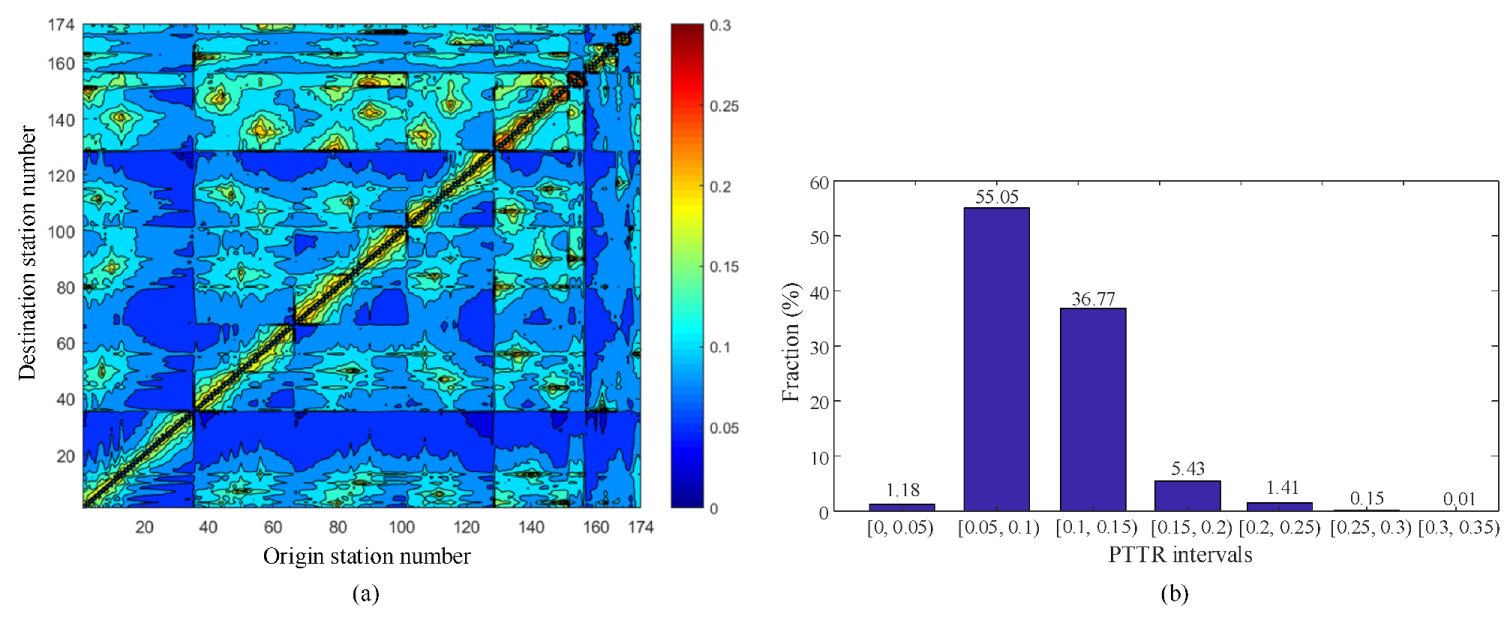
The PTRs among OD pairs are estimated according to the proposed metrics and method. The contours of PTRs among OD pairs in Chengdu’s RTN during morning peak hours are shown in Figure 7a. Figure 7a shows the PTRs among OD pairs are between 0 to 0.3, which means that passengers should allow 0 to 0.3 times the average PTT to reach their destinations reliably. Figure 7b shows the fractions of OD pairs in different PTR intervals during morning peak periods. It shows that only 1.57% of OD pairs’ PTRs exceed 0.2, which demonstrates that only a few OD pairs have low PTR.
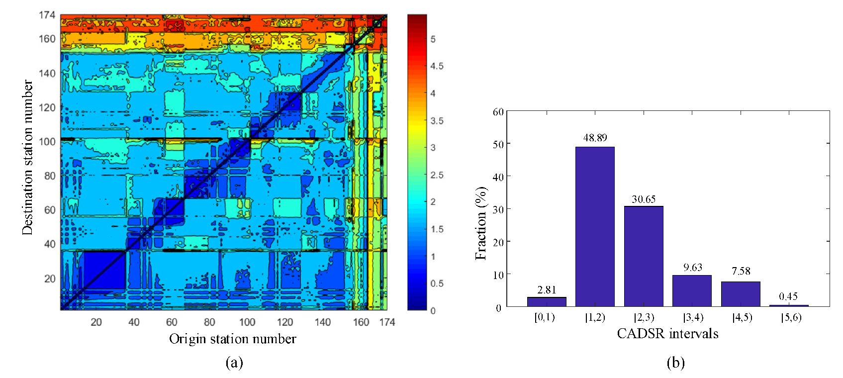
The PTRCs among OD pairs are estimated according to PTRs among OD pairs. The contours of PTRCs among OD pairs and the fractions of OD pairs in different PTRC intervals are shown in Figure 8a,b, respectively, on Chengdu’s RTN during morning peak hours. Figure 8a shows the PTRCs among OD pairs are between 0.72 ¥ to 5 ¥. It means that the extra costs of arriving at destination stations reliably for a passenger are between 0.72 ¥ to 5.98 ¥. The stations whose numbers exceed 156 are on suburban and high-speed railways. Figure 8a shows PTRCs among Metro, suburban railway, and high-speed railway are high. Figure 8b shows the fractions of OD pairs in different PTRC intervals during morning peak periods. It shows that nearly 80% of OD pairs’ PTRCs are between 1 ¥ and 3 ¥.
4.3.2. PTRs and the PTRCs on Lines and on the RTN
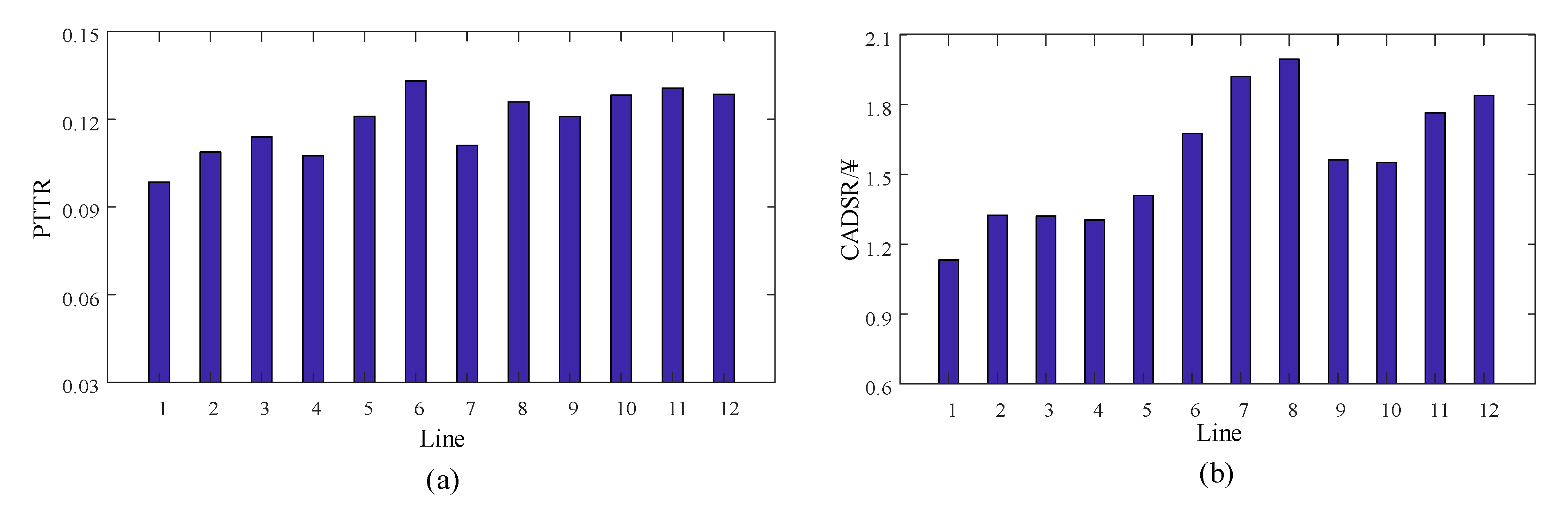
The PTRs and PTRCs on lines during morning peak hours are estimated with Equations (16) and (17). They are shown in Figure 9a,b, respectively. A higher value of the PTR indicates lower reliability. The PTR on line 6 is the lowest and PTRC on line 8 is the highest in Figure 9a,b, respectively. Therefore, with limited operational resources and manpower, priority can be given to improving the management of lines with a high value of PTR and high PTRC to increase passengers’ PTR and decrease the passengers’ PTRC.
The PTR and PTRC on Chengdu’s RTN during morning peak hours are estimated to be 0.14, and 2.07 ¥, respectively. Therefore, on average, passengers should allow 0.14 of the mean PTT (equivalent to 2.07 ¥) to arrive at their destination stations reliably. The fare per passenger trip is 6.08 ¥ in Chengdu’s RTN during morning peak hours. Therefore, a passenger must spend over 1/3 of the basic travel fare in equivalent extra time to reach the destination station reliably.
4.4. Regression Analysis Relating PTRs and PTRCs to Influential Factors
4.4.1. Regression Models Relating PTR and PTRC to Influential Factors
The regression models relating PTR and PTRC to influential factors are proposed. In theory, more influential factors in a regression model increase its degree of fit and interpretability. However, no model can include all the influential factors due to possible multicollinearity. Besides, too many factors in a regression model will lead to model overfitting. The factors that are closely related to passengers’ PTT and can be quantified are considered. Six influential factors (i.e., explanatory variables), which are the distances of paths , walking distances on paths , the average trip times on paths , the average waiting times on paths , average loading factor on paths’ links and ratios of walking distances on paths to distances of paths are considered in developing multiple linear regression models:
where and are PTRs and PTRCs on paths, respectively. to and to are regression coefficients for each explanatory variable. means the change in the mean of PTR corresponding to a unit change in when other variables are held constant. means the change in the mean of PTRC corresponding to a unit change in when other variables are held constant. and are constant values. and represent models’ error, which are random variables and whose mean is 0.
The influential factors in the multiple linear regression models may have correlations among them. In addition, not all influential factors significantly influence the PTRs or PTRCs. The stepwise regression method [11] is used here to reduce multicollinearity among influential factors. It gradually introduces influential factors that have a high impact on the PTRs or PTRCs into the regression models. During the process of introducing the factors into a regression model, the significance test is performed for the new model when a new factor is introduced into it.
4.4.2. Multiple Linear Regression Analysis for PTRs and Influential Factors
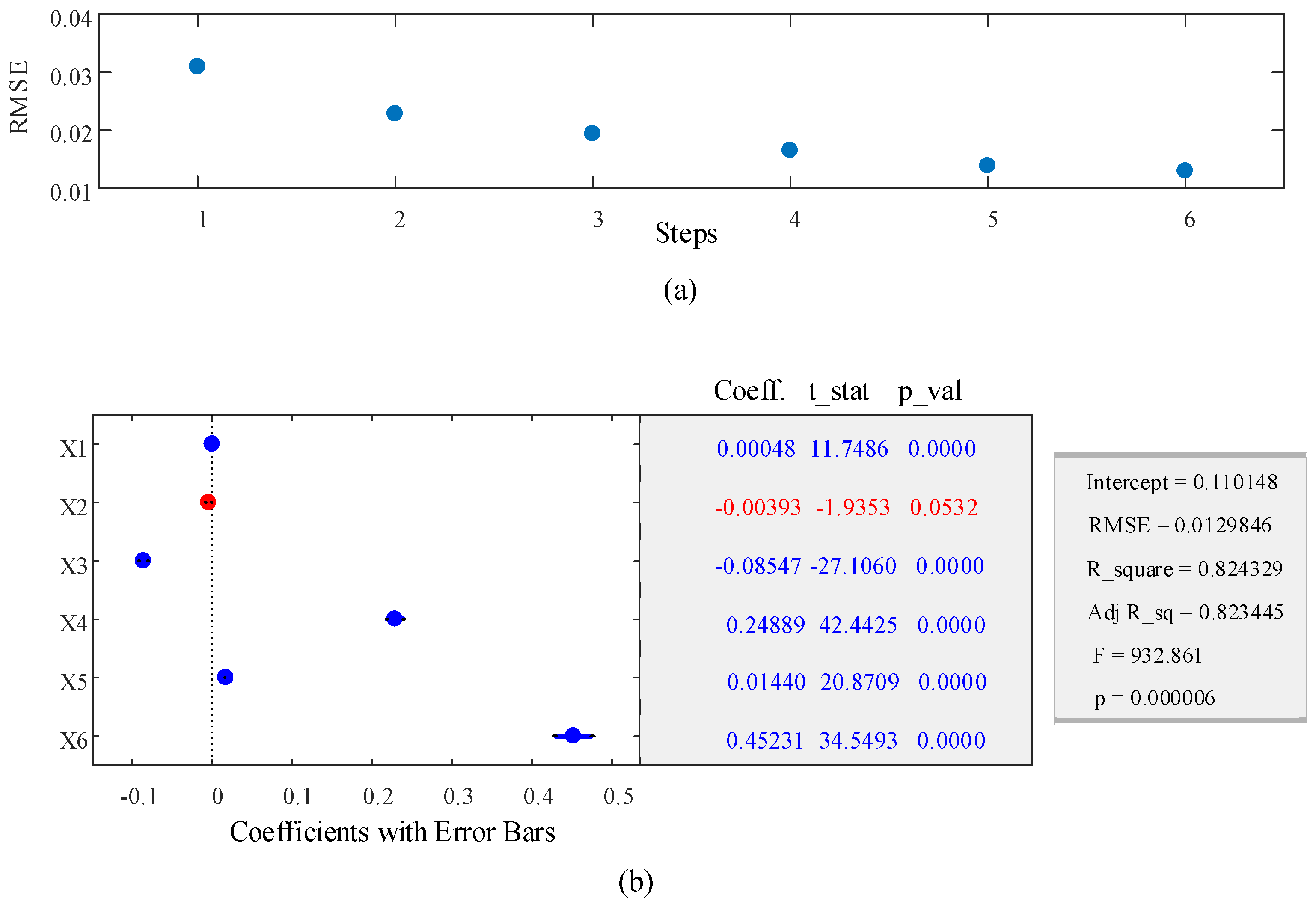
The result of applying the stepwise regression method to determine the appropriate multiple linear regression model among PTRs and influential factors is shown in Figure 10. Figure 10a demonstrates that with additional stepwise regression iterations, the root mean square error (RMSE) decreases and the model fitting improves. The result of applying the stepwise regression method shows that all factors except (walking distances on paths) are included in the model. The multiple linear regression model is shown in Equation (31). The significance value of the model (i.e., the value of in Figure 10b) is 6 × 10⁻⁶, which is below 0.05 (0.05 is a commonly used value for judging whether the significance test is passed). This demonstrates that the linear relation between PTR and influential factors is significant. The coefficient of determination (i.e., R_square in Figure 10b) that quantifies the degree of linear correlation is 0.82433. It indicates that Equation (31) has a high goodness-of-fit.
4.4.3. Multiple Linear Regression Analysis for PTRC and Influential Factors
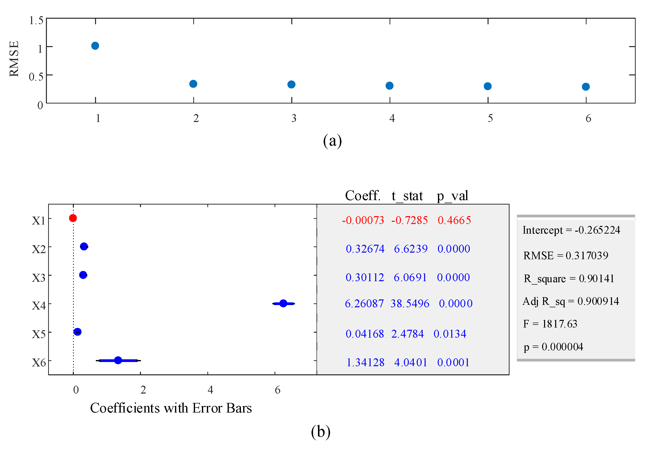
Figure 11 shows the RMSE after introducing factors into the regression model and the result of applying the stepwise regression for determining the appropriate multiple linear regression model that relates PTRC to influential factors. Figure 11a demonstrates that applying the stepwise regression method can improve the fit of the model. The result of applying the stepwise regression method shows that (distances of paths) is not introduced into the multiple linear regression model; 4 × 10⁻⁶ (i.e., the value of in Figure 11b) is the significance value of the model, which is below 0.05 (0.05 is a commonly used value for judging whether the significance test is passed). Therefore, the linear relation between PTRC and influential factors is significant. R_square in Figure 11b is 0.9014. It is close to 1 and thus demonstrates that Equation (32) has a high goodness-of-fit. The multiple linear regression model between PTRC and influential factors is shown in Equation (32).
4.4.4. PTR Enhancement and PTRC Reduction Analysis
The absolute coefficients’ values for and are much larger than the coefficient values for other influential factors in Equations (31) and (32). This means that the average waiting times on paths () and the ratios of walking distances on paths to distances of paths () have a much higher influence on paths’ PTRs and PTRCs than other influential factors. A higher value of means a lower PTR. In order to decrease the and and thus to enhance PTR as well as reduce PTRC on the network, the values of and should be decreased. The percent decreases in and are shown in Figure 12 when the values of and are decreased.
Figure 12 shows that reducing the values of and is effective in decreasing and . Therefore, two ways for improving the PTR and decreasing PTRC on the RTN are proposed: (1) decreasing the headway on lines to decrease the average waiting time on paths, and (2) providing convenient facilities and channels for passengers to enter, exit, and transfer at the stations, thereby decreasing the walking distances on paths.
5. Conclusions
Time reliability is one of the most important factors affecting the passengers’ satisfaction with transportation services. The assessment of time reliability has attracted considerable attention. However, the existing literature on time reliability neglects the passengers’ travel conditions since the clock-based trip time, which does not contain travel conditions, is used for measuring time reliability. This study measures the PTR according to the passengers’ PTTs, which reflect passengers’ travel conditions (crowding and seat availability in the vehicle and the number of transfer times on the path). The metrics for estimating PTRs and the cost passengers pay for reaching destination reliably (PTRCs) are developed. Due to the difficulty of obtaining passengers’ trip time traveling among multiple modes of rail transit, a Monte Carlo simulation is used here for estimating PTTR and PTRC that does not rely on massive passenger travel data and data analysis. The multiple linear regression models relating PTR and PTRC to influential factors are developed and determined by applying the stepwise regression method. The following conclusions are drawn from applying proposed models and method to Chengdu’s RTN during morning peak hours:
Only a few OD pairs on Chengdu’s RTN during morning peak hours have low PTR. Nearly 80% of OD pairs’ PTRCs are between 1 ¥ and 3 ¥. The PTR on line 6 is the lowest, and PTRC on line 8 is the highest. The PTR and PTRC on Chengdu’s RTN are estimated to be 0.14, and 2.07 ¥, respectively. A passenger must allow 0.14 of the average PTT and spend over 1/3 of travel fare in equivalent extra PTT to reach the destination station reliably.
The linear relations among PTR, PTRC, and their influential factors are significant. The obtained multiple linear regression models have high goodness-of-fit. The average waiting times on paths and the ratios of walking distances on paths to distances of paths affect PTR and PTRC much more than other factors. Decreasing the headway on lines decreases the average waiting time on paths, and providing convenient facilities and channels for passengers to enter, exit, and transfer at the stations to decrease the walking distances on paths are effective in enhancing PTR and reducing the PTRC in an RTN.
The proposed models and method can measure PTR and PTRC in an RTN network by integrating travel conditions and trip time. According to the evaluation results, the lines with low PTR and with high PTRC can be identified, which helps operators allocate operational resources and manpower to those lines with high priority to improve PTR and reduce PTRC. The influences of factors on PTR and PTRC are quantified according to obtained multiple linear regression models, which not only help guide operators in effectively improving the PTR and reducing the PTRC in an RTN, but also guides passengers to prepare extra PTT and select a path with high PTR. Although the metrics and method only apply to an RTN, they can potentially apply to different transportation modes, such as bus networks.
Although crowding level of trains, seat availability, and transfer times are considered here to measure PTR, other factors that affect the time reliability, such as the stability of the transportation and the probability of the transportation disturbances should be considered in further studies. Many passengers require transfers among multiple public transportation lines, such as rail transit and bus. Therefore, the PTR and PTRC evaluation should be extended to public transportation networks that include rail transit and bus lines.
Author Contributions
Conceptualization, J.L. and P.S.; methodology, J.L. and Y.Y.; software, J.C.; validation, J.L., J.C. and Y.Y.; formal analysis, Y.Y.; investigation, J.L., J.C. and Y.Y.; resources, Q.P.; data curation, Y.Y.; writing—original draft preparation, J.L. and Y.Y.; writing—review and editing, P.S. and Y.Y.; visualization, J.C.; supervision, Q.P.; project administration, Q.P.; funding acquisition, Q.P. All authors have read and agreed to the published version of the manuscript.
Funding
This research was funded by the National Key R & D Program of China, grant number 2017YFB1200700, and the China Scholarship Council, grant number 201907000071.
Institutional Review Board Statement
Not applicable.
Informed Consent Statement
Not applicable.
Data Availability Statement
The data presented in this study are available on request from the corresponding author.
Acknowledgments
The authors thank the Chengdu’s rail transit manager for providing relevant data. We also acknowledge the support of the National Key R & D Program of China (2017YFB1200700), The first author is supported by the China Scholarship Council (No.201907000071).
Conflicts of Interest
The authors declare no conflict of interest.
References
- Moghaddam, Z.R.; Jeihani, M.; Peeta, S.; Banerjee, S. Comprehending the roles of traveler perception of travel time reliability on route choice behavior. Travel Behav. Soc. 2019, 16, 13–22. [Google Scholar] [CrossRef]
- Beirão, G.; Cabral, J.S. Understanding attitudes towards public transport and private car: A aualitative study. Transp. Policy 2007, 14, 478–489. [Google Scholar] [CrossRef]
- Li, Z.; Hensher, D.A.; Rose, J.M. Willingness to pay for travel time reliability in passenger transport: A review and some new empirical evidence. Transp. Res. Part E Logist. Transp. Rev. 2010, 46, 384–403. [Google Scholar] [CrossRef]
- De Jong, G.C.; Bliemer, M.C. On including travel time reliability of road traffic in appraisal. Transp. Res. Part A Policy Pr. 2015, 73, 80–95. [Google Scholar] [CrossRef]
- Li, X.; Liu, L.; Mu, H. Evaluation of road network total travel time reliability based on fourth-moment. J. Transp. Syst. Eng. Inf. Technol. 2019, 19, 145–150. [Google Scholar]
- Sun, Y.; Shi, J.; Schonfeld, P.M. Identifying passenger flow characteristics and evaluating travel time reliability by visualizing AFC data: A case study of Shanghai Metro. Public Transp. 2016, 8, 341–363. [Google Scholar] [CrossRef]
- Liu, J.; Schonfeld, P.M.; Peng, Q.; Yin, Y. Measures of Travel Reliability on an Urban Rail Transit Network. J. Transp. Eng. Part A Syst. 2020, 146, 04020037. [Google Scholar] [CrossRef]
- Ma, Z.-L.; Ferreira, L.; Mesbah, M.; Hojati, A.T.; Information, R. Modeling Bus Travel Time Reliability with Supply and Demand Data from Automatic Vehicle Location and Smart Card Systems. Transp. Res. Rec. J. Transp. Res. Board 2015, 2533, 17–27. [Google Scholar] [CrossRef]
- Uno, N.; Kurauchi, F.; Tamura, H.; Iida, Y. Using Bus Probe Data for Analysis of Travel Time Variability. J. Intell. Transp. Syst. 2009, 13, 2–15. [Google Scholar] [CrossRef] [Green Version]
- Jenelius, E. Public transport experienced service reliability: Integrating travel time and travel conditions. Transp. Res. Part A Policy Pr. 2018, 117, 275–291. [Google Scholar] [CrossRef] [Green Version]
- Jennrich, R.I.; Sampson, P.F. Application of stepwise regression to non-linear estimation. Technometrics 1968, 10, 63–72. [Google Scholar] [CrossRef]
- De Oliveira, E.L.; Portugal, L.D.S.; Junior, W.P. Indicators of reliability and vulnerability: Similarities and differences in ranking links of a complex road system. Transp. Res. Part A Policy Pr. 2016, 88, 195–208. [Google Scholar] [CrossRef]
- Wakabayashi, H.; Matsumoto, Y. Comparative study on travel time reliability indexes for highway users and operators. J. Adv. Transp. 2012, 46, 318–339. [Google Scholar] [CrossRef]
- Van Loon, R.; Rietveld, P.; Brons, M. Travel-time reliability impacts on railway passenger demand: A revealed preference analysis. J. Transp. Geogr. 2011, 19, 917–925. [Google Scholar] [CrossRef]
- Lyman, K.; Bertini, R. Using Travel Time Reliability Measures to Improve Regional Transportation Planning and Operations. Transp. Res. Rec. J. Transp. Res. Board 2008, 2046, 1–10. [Google Scholar] [CrossRef] [Green Version]
- Rietveld, P.; Bruinsma, F.R.; van Vuuren, D.J. Coping with unreliability in public transport chains: A case study for Netherlands. Transp. Res. Part A Policy Pr. 2001, 35, 539–559. [Google Scholar] [CrossRef]
- Ma, Z.; Ferreira, L.; Mesbah, M. A framework for the development of bus service reliability measures. In Proceedings of the Presentation to Transport Research Forum 2013, Brisbane, Australia, 2–4 October 2013. [Google Scholar]
- Woodard, D.; Nogin, G.; Koch, P.; Racz, D.; Goldszmidt, M.; Horvitz, E. Predicting travel time reliability using mobile phone GPS data. Transp. Res. Part C Emerg. Technol. 2017, 75, 30–44. [Google Scholar] [CrossRef]
- Rakha, H.; El-Shawarby, I.; Arafeh, M. Trip Travel-Time Reliability: Issues and Proposed Solutions. J. Intell. Transp. Syst. 2010, 14, 232–250. [Google Scholar] [CrossRef]
- Uniman, D.L.; Attanucci, J.; Mishalani, R.G.; Wilson, N.H.M. Service reliability measurement using automated fare card data: Application to the London underground. Transp. Res. Rec. 2010, 2143, 92–99. [Google Scholar] [CrossRef] [Green Version]
- Ehrlich, J.E. Applications of Automatic Vehicle Location Systems Towards Improving Service Reliability and Operations Planning in London. Master’s Thesis, Massachusetts Institute of Technology, Cambridge, MA, USA, 2010. [Google Scholar]
- Wood, D.A. A Framework for Measuring Passenger-Experienced Transit Reliability Using Automated Data. Master’s Thesis, Massachusetts Institute of Technology, Cambridge, MA, USA, 2015. [Google Scholar]
- Pu, X. Analytic relationships between travel time reliability measures. Transp. Res. Rec. 2011, 2254, 122–130. [Google Scholar] [CrossRef]
- Van Lint, J.W.C.; van Zuylen, H.J.; Tu, H. Travel time unreliability on freeways: Why measures based on variance tell only half the story. Transp. Res. Part A Policy Pr. 2008, 42, 258–277. [Google Scholar] [CrossRef]
- Lomax, T.; Schrank, D.; Turner, S.; Margiotta, R. Selecting Travel Time Reliability Measures; Texas Transportation Institute: College Station, TX, USA, 2003. [Google Scholar]
- Furth, P.G.; Muller, T.H.J. Service Reliability and Hidden Waiting Time: Insights from Automatic Vehicle Location Data. Transp. Res. Rec. J. Transp. Res. Board 2006, 1955, 79–87. [Google Scholar] [CrossRef]
- Lo, H.K.; Luo, X.W.; Siu, B.W.Y. Degradable transport network: Travel time budget of travelers with heterogeneous risk aversion. Transp. Res. Part B Methodol. 2006, 40, 792–806. [Google Scholar] [CrossRef]
- Xu, X.; Chen, A.; Cheng, L.; Lo, H.K. Modeling distribution tail in network performance assessment: A mean-excess total travel time risk measure and analytical estimation method. Transp. Res. Part B Methodol. 2014, 66, 32–49. [Google Scholar] [CrossRef]
- Zheng, F.; Liu, X.; van Zuylen, H.V.; Li, J.; Lu, C. Travel Time Reliability for Urban Networks: Modelling and Empirics. J. Adv. Transp. 2017, 2017, 9147356. [Google Scholar] [CrossRef] [Green Version]
- Al-Deek, H.; Emam, E.B. New Methodology for Estimating Reliability in Transportation Networks with Degraded Link Capacities. J. Intell. Transp. Syst. 2006, 10, 117–129. [Google Scholar] [CrossRef]
- Kim, J.; Mahmassani, H.S.; Vovsha, P.; Stogios, Y.; Dong, J. Scenario-Based Approach to Analysis of Travel Time Reliability with Traffic Simulation Models. Transp. Res. Rec. J. Transp. Res. Board 2013, 2391, 56–68. [Google Scholar] [CrossRef] [Green Version]
- Wang, J.; Gao, X.; Sun, Z. A Multilevel Simulation Method for Time-Variant Reliability Analysis. Sustainability 2021, 13, 3646. [Google Scholar] [CrossRef]
- Bruzelius, N.A. Microeconomic theory and generalised cost. Transportmetrica 1981, 10, 233–245. [Google Scholar] [CrossRef]
- Litman, T. Valuing transit service quality improvements. J. Public Transp. 2008, 11, 43–63. [Google Scholar] [CrossRef] [Green Version]
- Qian, K.; Chen, Y.; Mao, B.H. Route choice behavior for urban rail transit considering transfer time. J. Transp. Syst. Eng. Inf. Technol. 2015, 15, 116–121. [Google Scholar]
- Wardman, M.; Whelan, G. Twenty years of rail crowding valuation studies: Evidence from lessons from British experience. Transp. Rev. 2011, 31, 379–398. [Google Scholar] [CrossRef]
- Kim, Y.-J. Monte Carlo vs. Fuzzy Monte Carlo Simulation for Uncertainty and Global Sensitivity Analysis. Sustainability 2017, 9, 539. [Google Scholar] [CrossRef] [Green Version]
- Zhao, Y. On Interchange of Urban Rail Transit Considering Level of Service. Ph.D. Thesis, Beijing Jiaotong University, Beijing, China, 2011. (In Chinese). [Google Scholar]
- Dixit, M.; Brands, T.; van Oort, N.; Cats, O.; Hoogendoorn, S. Passenger Travel Time Reliability for Multimodal Public Transport Journeys. Transp. Res. Rec. J. Transp. Res. Board 2019, 2673, 149–160. [Google Scholar] [CrossRef] [Green Version]
- Sun, Y.; Xu, R. Rail transit travel time reliability and estimation of passenger route choice behavior: Analysis using automatic fare collection data. Transp. Res. Rec. 2012, 2275, 58–67. [Google Scholar] [CrossRef]
- Ingvardson, J.B.; Nielsen, O.A.; Raveau, S.; Nielsen, B.F. Passenger arrival and waiting time distributions dependent on train service frequency and station characteristics: A smart card data analysis. Transp. Res. Part C Emerg. Technol. 2018, 90, 292–306. [Google Scholar] [CrossRef] [Green Version]
- Liu, H.X.; He, X.; He, B. Method of Successive Weighted Averages (MSWA) and Self-Regulated Averaging Schemes for Solving Stochastic User Equilibrium Problem. Netw. Spat. Econ. 2009, 9, 485–503. [Google Scholar] [CrossRef]
- Zhou, Z.; Chen, A.; Bekhor, S. C-logit stochastic user equilibrium model: Formulations and solution algorithm. Transportation 2012, 8, 17–41. [Google Scholar] [CrossRef]
- Cascetta, E. Transportation Systems Engineering: Theory and Methods; Kluwer Academic Publishers: Dordrecht, The Netherlands, 2001. [Google Scholar]
- Zhou, F.; Xu, R.-H. Model of Passenger Flow Assignment for Urban Rail Transit Based on Entry and Exit Time Constraints. Transp. Res. Rec. J. Transp. Res. Board 2012, 2284, 57–61. [Google Scholar] [CrossRef]
- Litman, T. Transportation Cost and Benefit Analysis-Techniques, Estimates and Implications, 2nd ed.; Victoria Transport Policy Institute: Victoria, BC, Canada, 2009. [Google Scholar]
- Chengdu Bureau of Statistics. Chengdu Statistical Yearbook; China Statistics Press: Beijing, China, 2018. [Google Scholar]
Figure 1.
The clock-based trip time components.

Figure 2.
The steps for generating PTTs from station to station on path .

Figure 3.
(a) Chengdu’s RTN network; (b) Chengdu’s Metro network.

Figure 4.
Passenger trips among OD pairs during morning peak periods.

Figure 5.
Two paths from station 155 to station 13.

Figure 6.
(a) Cumulative distribution of generated 1000 passengers’ PTTs on path 1; (b) Cumulative distribution of generated 1000 passengers’ PTTs on path 1.
Figure 6.
(a) Cumulative distribution of generated 1000 passengers’ PTTs on path 1; (b) Cumulative distribution of generated 1000 passengers’ PTTs on path 1.

Figure 7.
(a) PTRs among OD pairs; (b) Fractions of OD pairs in different PTR intervals.

Figure 8.
(a) PTRCs among OD pairs; (b) Fractions of OD pairs in different PTRC intervals.

Figure 9.
(a) PTRs on lines; (b) CADRs on lines.

Figure 10.
(a) The value of RMSE when introducing influential factors into the model; (b) The result of applying the stepwise regression method.
Figure 10.
(a) The value of RMSE when introducing influential factors into the model; (b) The result of applying the stepwise regression method.

Figure 11.
(a) The value of RMSE when introducing influential factors into the model; (b) The result of applying the stepwise regression method.
Figure 11.
(a) The value of RMSE when introducing influential factors into the model; (b) The result of applying the stepwise regression method.

Figure 12.
The percent decreases in and when the values of and are decreased.


Table 1.
Time reliability indicators and description.
| Indicators | Description |
|---|---|
| Coefficient of variation [23] | The ratio of the standard deviation to the mean. |
| Skewness of time [24] | The ratio of the difference between the 90th percentile trip time and 50th percentile trip time to the difference between the 50th percentile trip time and 10th percentile trip time. |
| 90th or 95th percentile trip time [25] | 90th or 95th percentile trip time used as the reliable trip time |
| Buffer time [26] | The difference between the average trip time and 95th percentile trip time. |
| Buffer time index [26] | The percentage of buffer time with respect to the average trip time. |
| On-time arrival [27] | The probability that a trip arrives within the trip time budget. |
| Time unreliability [25] | The fraction of late arriving trips. |
| Total time budget [27] | The minimum trip time threshold that satisfies a certain reliability requirement given by decision-makers at a certain confidence level. |
| Mean-excess total time [28] | The conditional expectation of trip times exceeding the corresponding total trip time budget at a given confidence level. |
Table 2.
Values of at different load factors when sitting or standing.
| Load Factor (%) | Sitting | Standing |
|---|---|---|
| 0–75 | 0.86 | ---- |
| 75–100 | 0.95 | ---- |
| 100–125 | 1.05 | 1.62 |
| 125–150 | 1.16 | 1.79 |
| 150–175 | 1.27 | 1.99 |
| 175–200 | 1.40 | 2.20 |
| >200 | 1.55 | 2.44 |
Table 3.
Values of and for walking speed distribution [38].
Table 3.
Values of and for walking speed distribution [38].
| Walking Place | (m/s) | |
|---|---|---|
| passageways | 1.39 | 0.463 |
| upstairs | 0.79 | 0.236 |
| downstairs | 0.81 | 0.174 |
Table 4.
Values of parameters in Equation (9) for different headways.
| Headways (min) | ζ | ω | θ |
|---|---|---|---|
| 5 | 0.43 | 0.41 | 2.85 |
| 10 | 0.52 | 0.36 | 3.39 |
| 15 | 0.58 | 0.32 | 3.98 |
| 20 | 0.64 | 0.27 | 4.57 |
| 30 | 0.90 | 0.24 | 6.52 |
Table 5.
Attributes of Lines in Chengdu’s RTN.
| Line | Operation Type | Headway (min) | Seats (per Hour) | Capacity (Passenger Trips per Hour) |
|---|---|---|---|---|
| 1 | frequency-based | 2.00 | 348 × 30 | 1460 × 30 |
| 2 | frequency-based | 2.73 | 348 × 22 | 1460 × 22 |
| 3 | frequency-based | 3.00 | 348 × 20 | 1460 × 20 |
| 4 | frequency-based | 3.00 | 348 × 20 | 1460 × 20 |
| 5 | frequency-based | 4.00 | 348 × 15 | 1460 × 15 |
| 6 | frequency-based | 6.00 | 348 × 10 | 1460 × 10 |
| 7 | schedule-based | 10.00 | 250 × 6 | 680 × 6 |
| 8 | schedule-based | 15.00 | 250 × 4 | 680 × 4 |
| 9 | schedule-based | 15.00 | 250 × 4 | 680 × 4 |
| 10 | schedule-based | 15.00 | 610 × 4 | 1280 × 4 |
| 11 | schedule-based | 10.00 | 610 × 6 | 1280 × 6 |
| 12 | schedule-based | 10.00 | 610 × 6 | 1280 × 6 |
Seats= seats per train × frequency of trains; Capacity = capacity of train × frequency of trains.
Table 6.
Transfer walking distances at line 1’s transfer stations.
| Transfer Station | Transfer Direction | Walking Distance (m) | Transfer Direction | Walking Distance (m) |
|---|---|---|---|---|
| 3 | Line 1 to line 5 | 178 | Line 5 to line 1 | 155 |
| 3 | Line 1 to line 7 | 237 | Line 7 to line 1 | 207 |
| 6 | Line 1 to line 4 | 252 | Line 4 to line 1 | 155 |
| 7 | Line 1 to line 2 | 215 | Line 2 to line 1 | 200 |
| 10 | Line 1 to line 3 | 200 | Line 3 to line 1 | 104 |
| 13 | Line 1 to line 5 | 252 | Line 5 to line 1 | 126 |
Table 7.
Train running times on line 1’s links.
| Link (Station–Station) | Running Time (min) | Link (Station–Station) | Running Time (min) | ||
|---|---|---|---|---|---|
| Upstream | Downstream | Upstream | Downstream | ||
| 1–2 | 1.87 | 1.88 | 18–19 | 1.35 | 1.33 |
| 2–3 | 2.08 | 2.07 | 19–20 | 1.38 | 1.37 |
| 3–4 | 1.47 | 1.47 | 20–21 | 1.57 | 1.57 |
| 4–5 | 1.57 | 1.58 | 21–22 | 1.95 | 1.92 |
| 5–6 | 1.22 | 1.25 | 22–23 | 1.50 | 1.50 |
| 6–7 | 1.35 | 1.33 | 23–24 | 1.83 | 1.83 |
| 7–8 | 1.15 | 1.20 | 24–25 | 1.70 | 1.78 |
| 8–9 | 1.15 | 1.17 | 25–26 | 1.78 | 1.77 |
| 9–10 | 1.32 | 1.32 | 26–27 | 1.93 | 1.93 |
| 10–11 | 1.27 | 1.28 | 27–28 | 2.00 | 2.25 |
| 11–12 | 1.35 | 1.33 | 28–29 | 1.75 | 1.50 |
| 12–13 | 1.40 | 1.45 | 29–30 | 1.77 | 1.77 |
| 13–14 | 1.63 | 1.63 | 30–31 | 1.58 | 1.58 |
| 14–15 | 1.50 | 1.50 | 31–32 | 1.50 | 1.50 |
| 15–16 | 1.17 | 1.17 | 32–33 | 1.33 | 1.33 |
| 16–17 | 1.20 | 1.20 | 33–34 | 1.87 | 1.87 |
| 17–18 | 1.78 | 1.78 | 34–35 | 2.00 | 2.00 |
Publisher’s Note: MDPI stays neutral with regard to jurisdictional claims in published maps and institutional affiliations. |
© 2021 by the authors. Licensee MDPI, Basel, Switzerland. This article is an open access article distributed under the terms and conditions of the Creative Commons Attribution (CC BY) license (https://creativecommons.org/licenses/by/4.0/).
Share and Cite
MDPI and ACS Style
Liu, J.; Schonfeld, P.; Chen, J.; Yin, Y.; Peng, Q. Perceived Trip Time Reliability and Its Cost in a Rail Transit Network. Sustainability 2021, 13, 7504. https://0-doi-org.brum.beds.ac.uk/10.3390/su13137504
AMA Style
Liu J, Schonfeld P, Chen J, Yin Y, Peng Q. Perceived Trip Time Reliability and Its Cost in a Rail Transit Network. Sustainability. 2021; 13(13):7504. https://0-doi-org.brum.beds.ac.uk/10.3390/su13137504
Chicago/Turabian StyleLiu, Jie, Paul Schonfeld, Jinqu Chen, Yong Yin, and Qiyuan Peng. 2021. "Perceived Trip Time Reliability and Its Cost in a Rail Transit Network" Sustainability 13, no. 13: 7504. https://0-doi-org.brum.beds.ac.uk/10.3390/su13137504
Note that from the first issue of 2016, this journal uses article numbers instead of page numbers. See further details here.