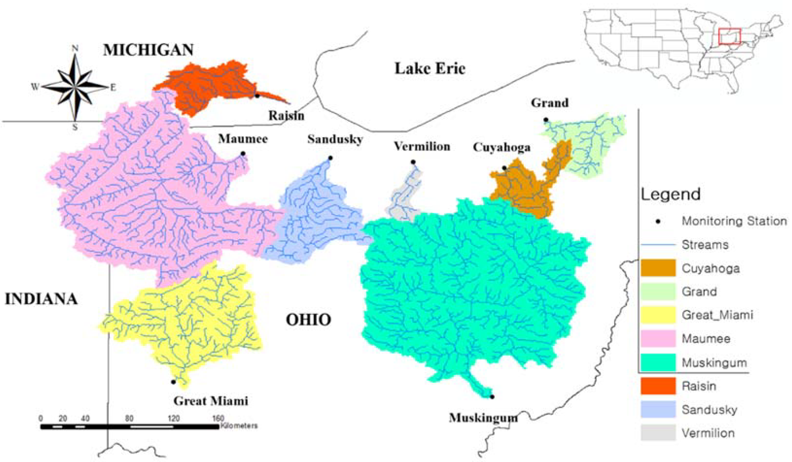
Figure 1.
Location of gaging stations and the corresponding watersheds used in this study.
Figure 1.
Location of gaging stations and the corresponding watersheds used in this study.
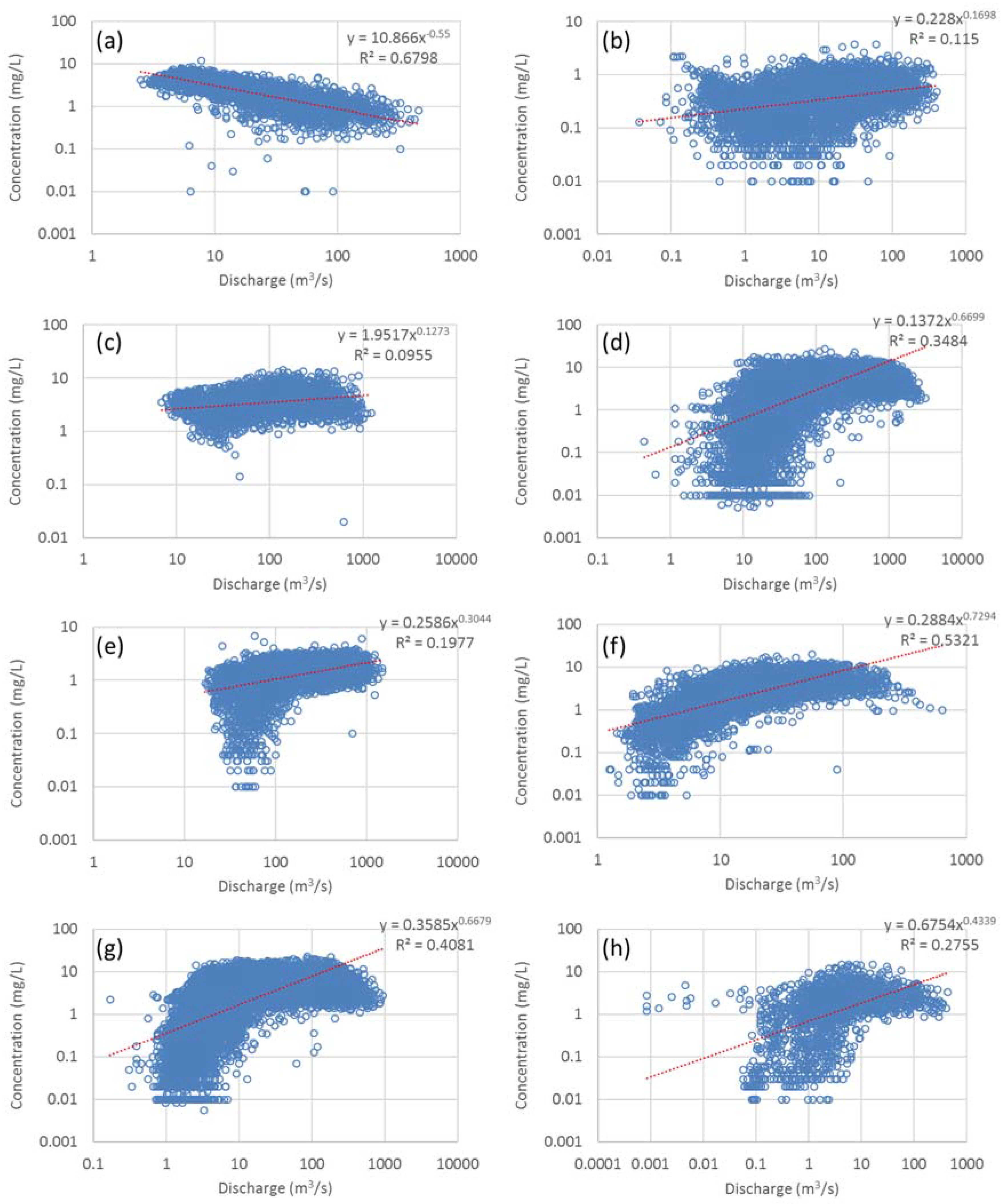
Figure 2.
Retrieved nitrate and streamflow data based on station: (a) Cuyahoga, (b) Grand, (c) Great Miami, (d) Maumee, (e) Muskingum, (f) Raisin, (g) Sandusky, and (h) Vermilion.
Figure 2.
Retrieved nitrate and streamflow data based on station: (a) Cuyahoga, (b) Grand, (c) Great Miami, (d) Maumee, (e) Muskingum, (f) Raisin, (g) Sandusky, and (h) Vermilion.
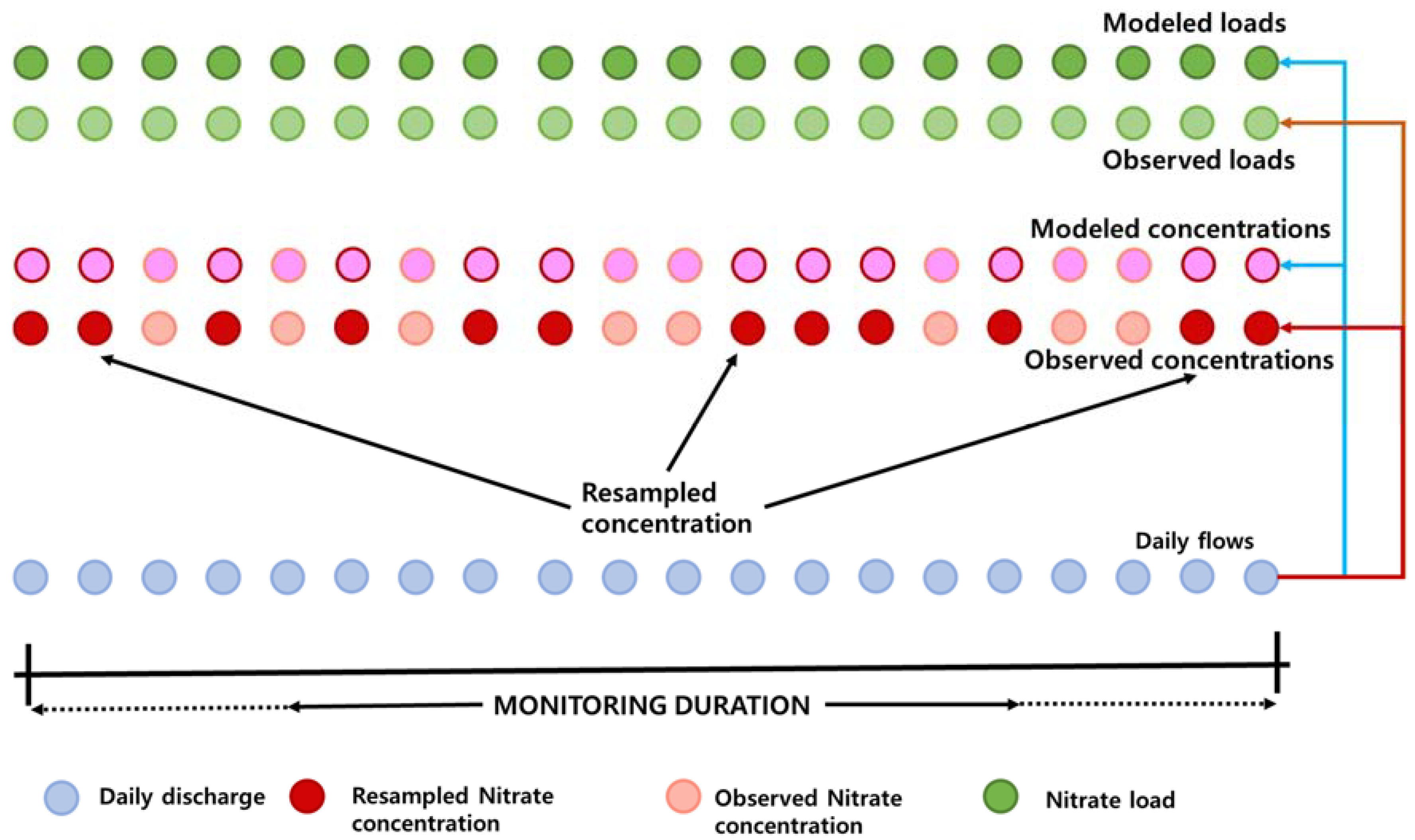
Figure 3.
Schematic diagram of comparisons between 23 estimation methods and “TRUE” estimation based on observed data with daily concentrations and loads.
Figure 3.
Schematic diagram of comparisons between 23 estimation methods and “TRUE” estimation based on observed data with daily concentrations and loads.
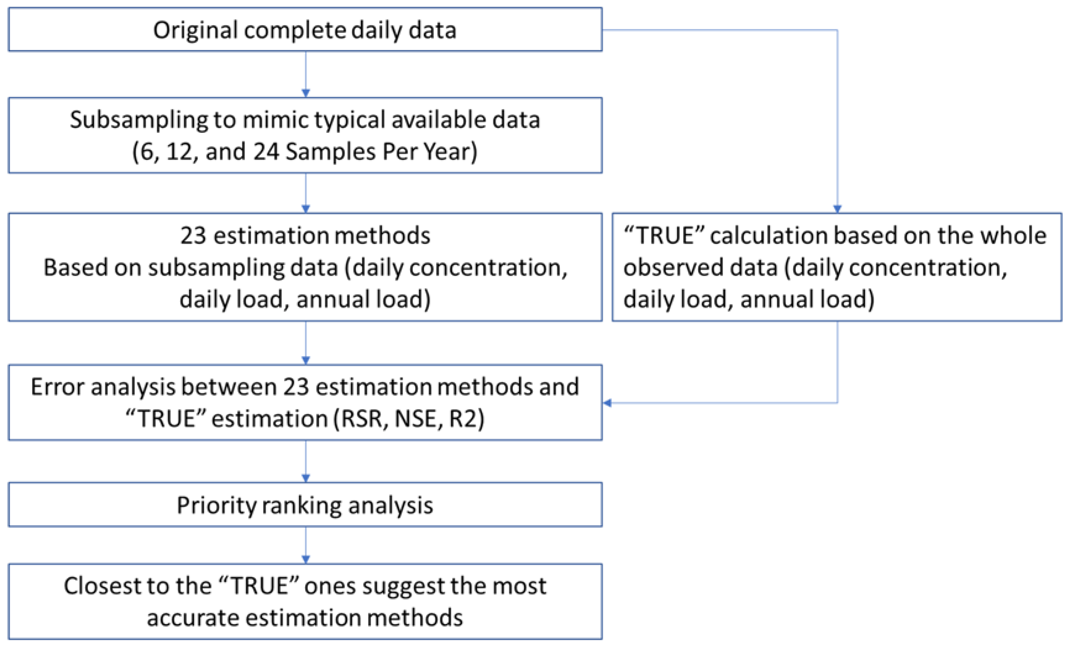
Figure 4.
Schematic of the load evaluation process in this study.
Figure 4.
Schematic of the load evaluation process in this study.
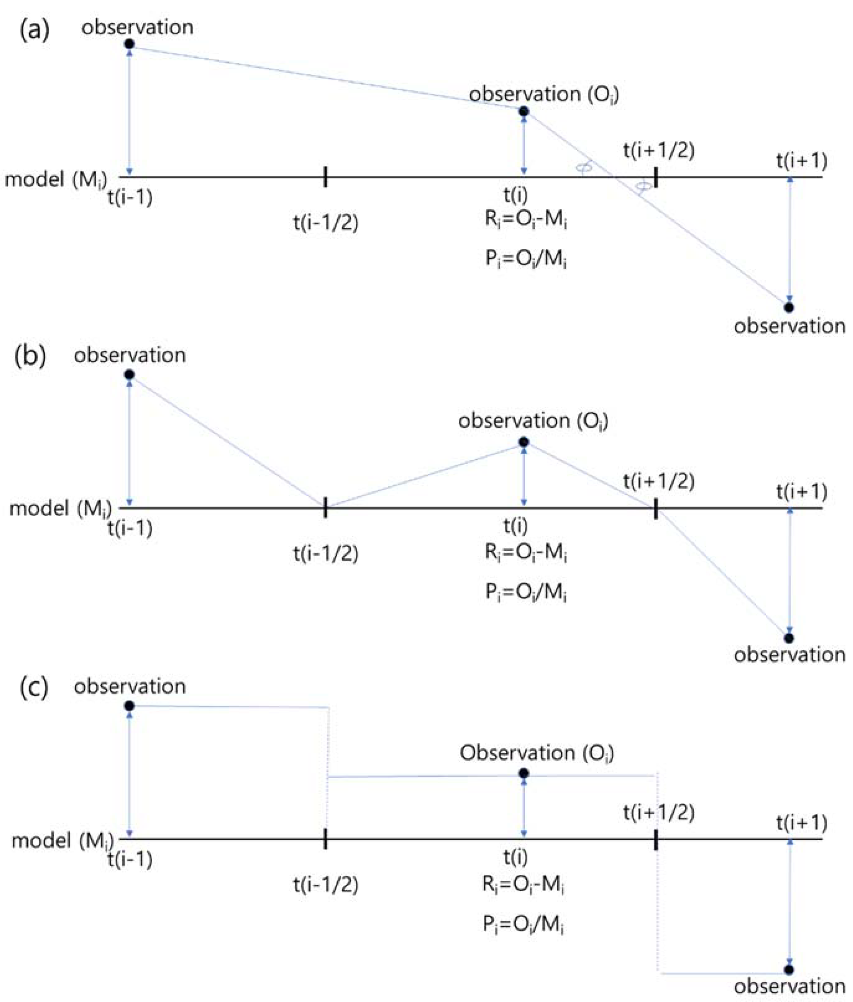
Figure 5.
Schematics of the three error-correction distributions for residual and proportional adjustments: (a) composite method (piecewise linear interpolation), (b) triangular distribution, and (c) rectangular distribution.
Figure 5.
Schematics of the three error-correction distributions for residual and proportional adjustments: (a) composite method (piecewise linear interpolation), (b) triangular distribution, and (c) rectangular distribution.
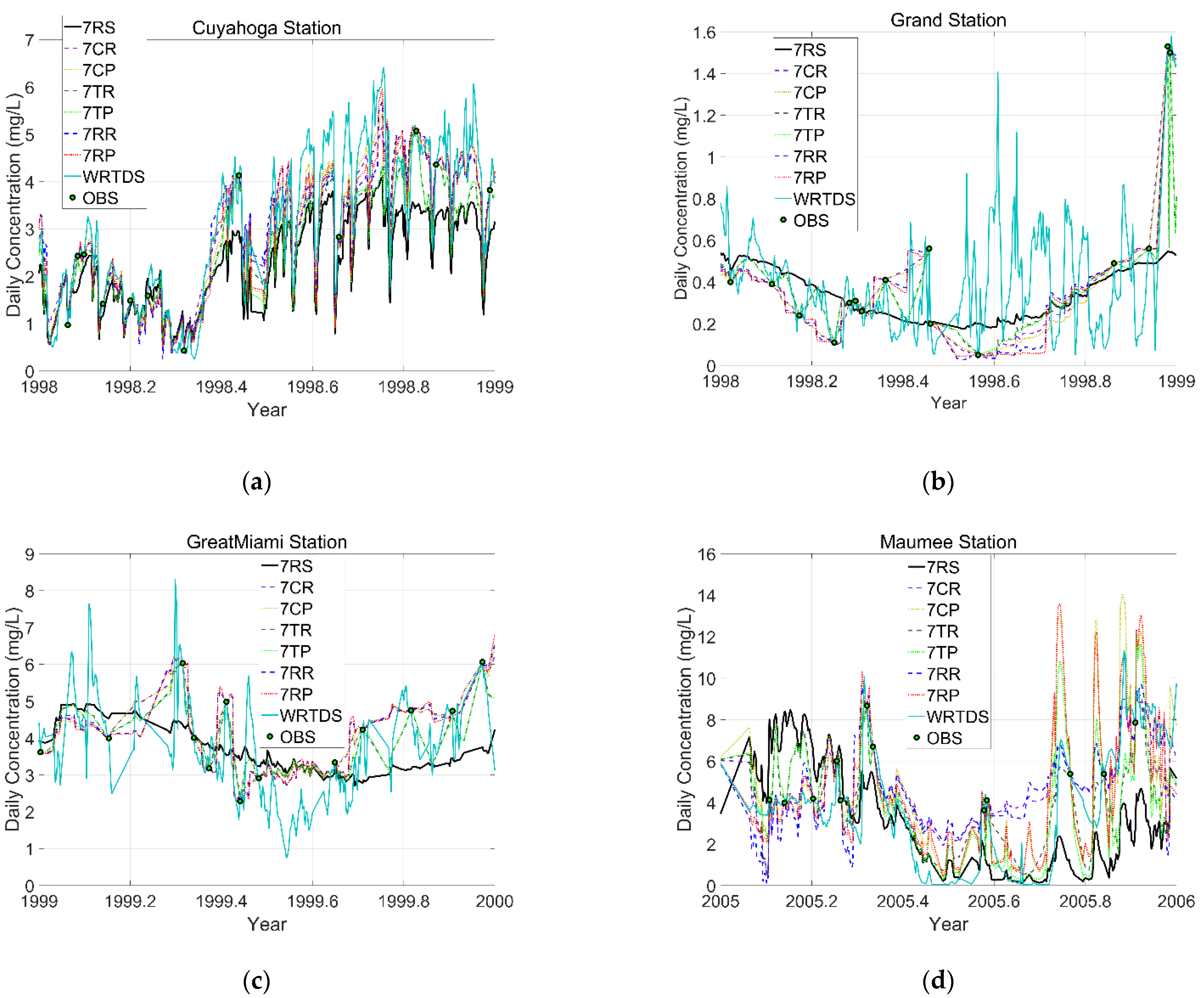
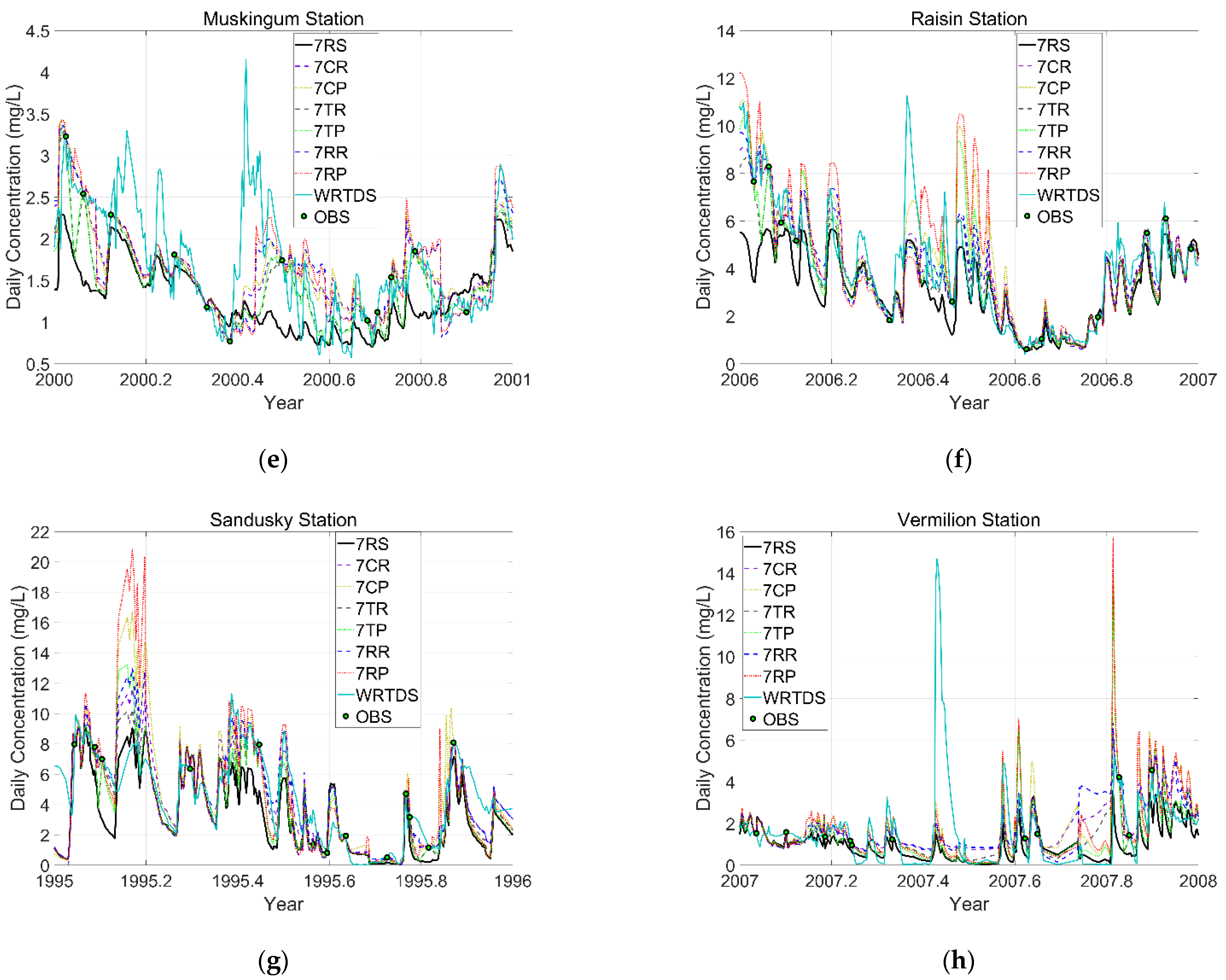
Figure 6.
Daily concentration estimates for 7-parameter estimation, 7-parameter with adjustment methods and WRTDS under the 12 observations per year condition in a particular year: (a) Cuyahoga, (b) Grand, (c) Great Miami, (d) Maumee, (e) Muskingum, (f) Raisin, (g) Sandusky, and (h) Vermilion.
Figure 6.
Daily concentration estimates for 7-parameter estimation, 7-parameter with adjustment methods and WRTDS under the 12 observations per year condition in a particular year: (a) Cuyahoga, (b) Grand, (c) Great Miami, (d) Maumee, (e) Muskingum, (f) Raisin, (g) Sandusky, and (h) Vermilion.
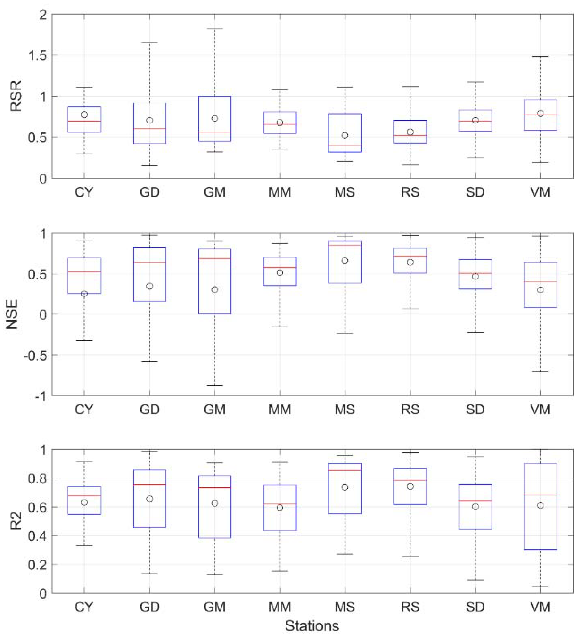
Figure 7.
Error analysis of all combining daily concentration, daily load and annual load performance results at eight stations (Note: circles indicate the mean value).
Figure 7.
Error analysis of all combining daily concentration, daily load and annual load performance results at eight stations (Note: circles indicate the mean value).
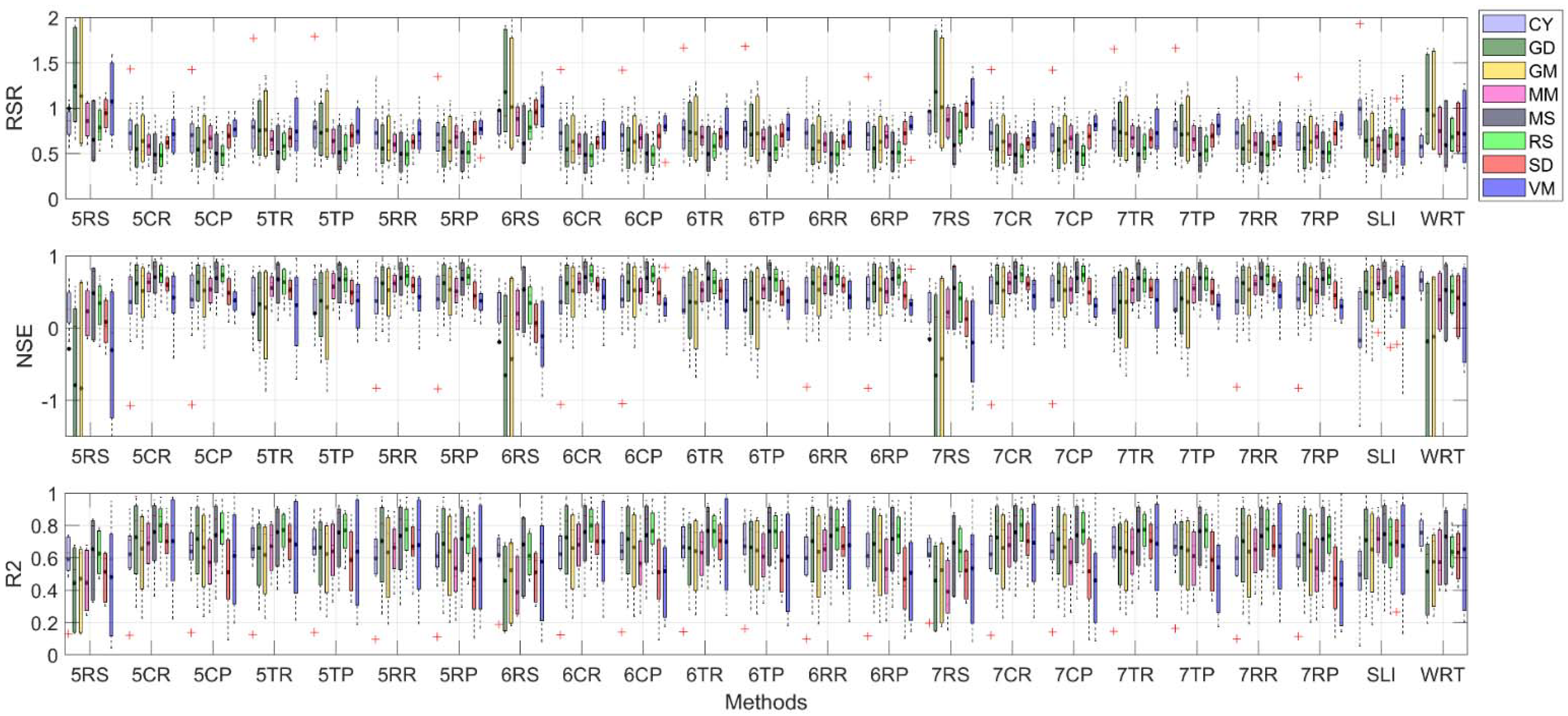
Figure 8.
Error analysis results of 23 estimation methods for individual stations (note: black points indicate the mean value).
Figure 8.
Error analysis results of 23 estimation methods for individual stations (note: black points indicate the mean value).
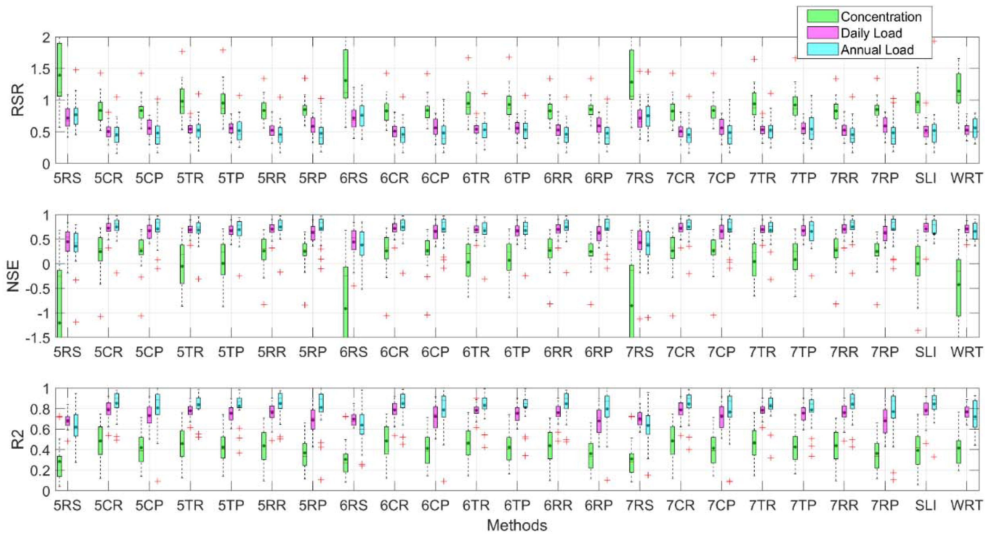
Figure 9.
Error analysis results of 23 estimation methods based on concentration, daily load, and annual load (note: black points indicate the mean value).
Figure 9.
Error analysis results of 23 estimation methods based on concentration, daily load, and annual load (note: black points indicate the mean value).
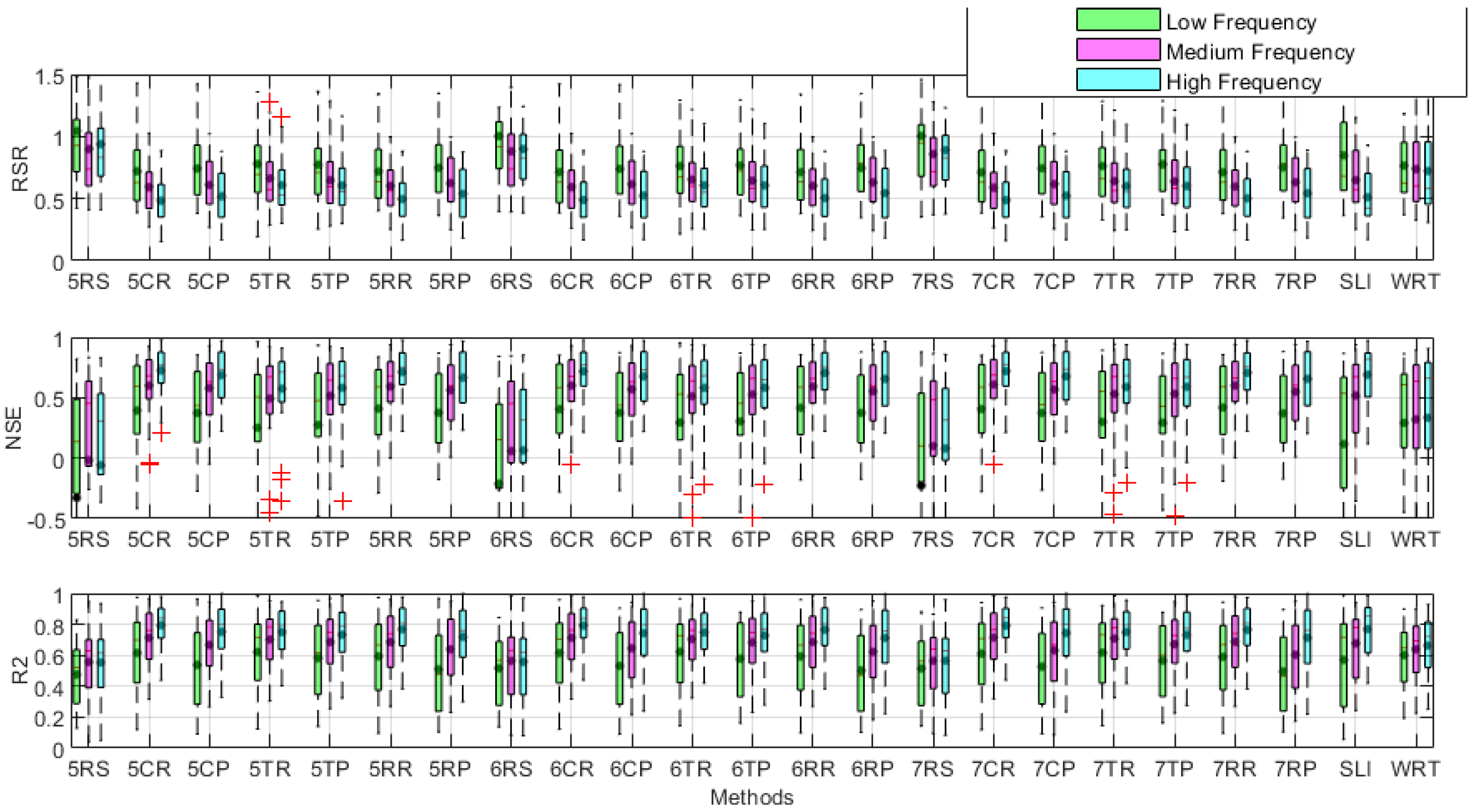
Figure 10.
Error analysis results of 23 estimation methods based on sampling frequencies and combined concentration, daily load, and annual load (note: black points indicate the mean value).
Figure 10.
Error analysis results of 23 estimation methods based on sampling frequencies and combined concentration, daily load, and annual load (note: black points indicate the mean value).
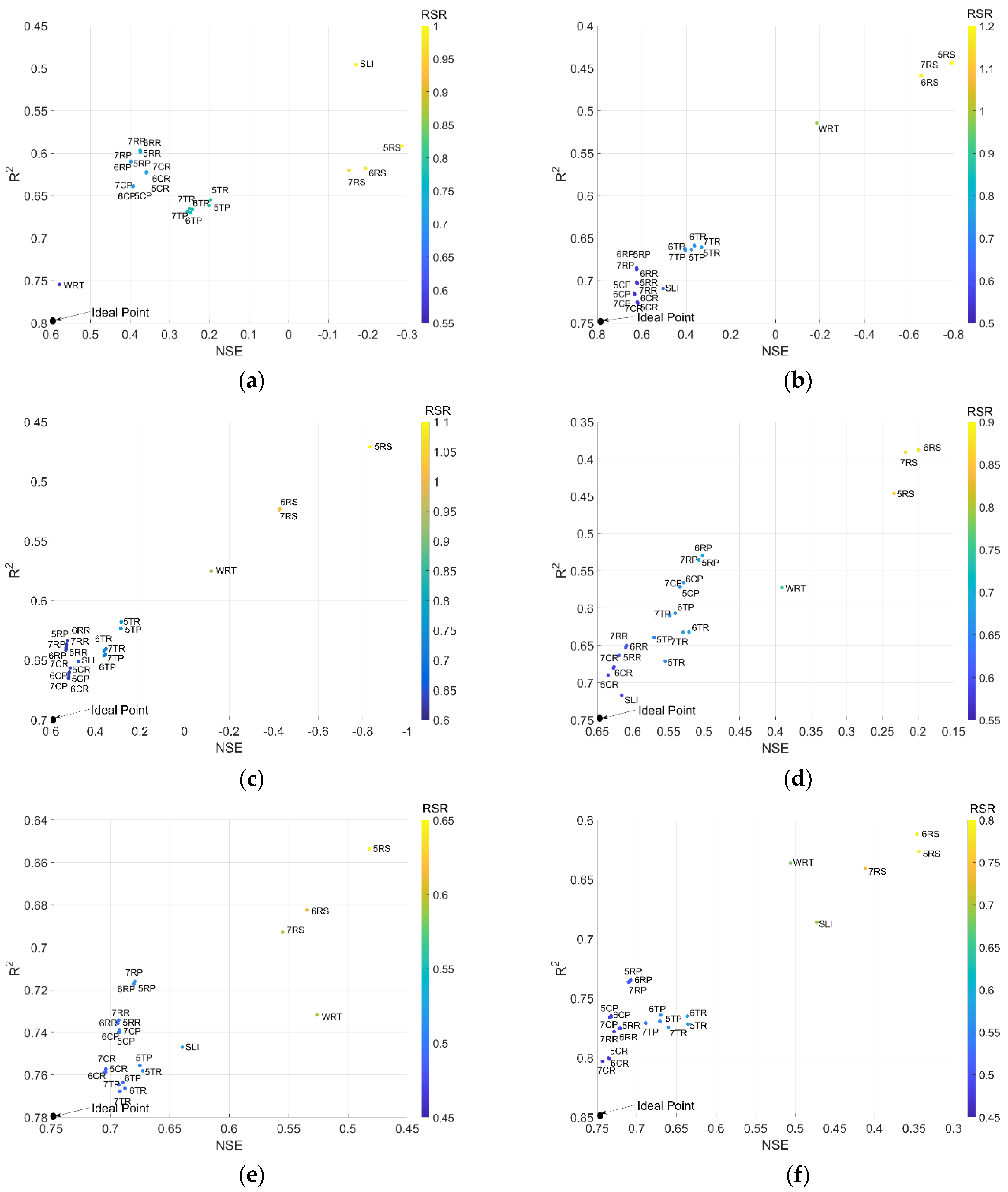
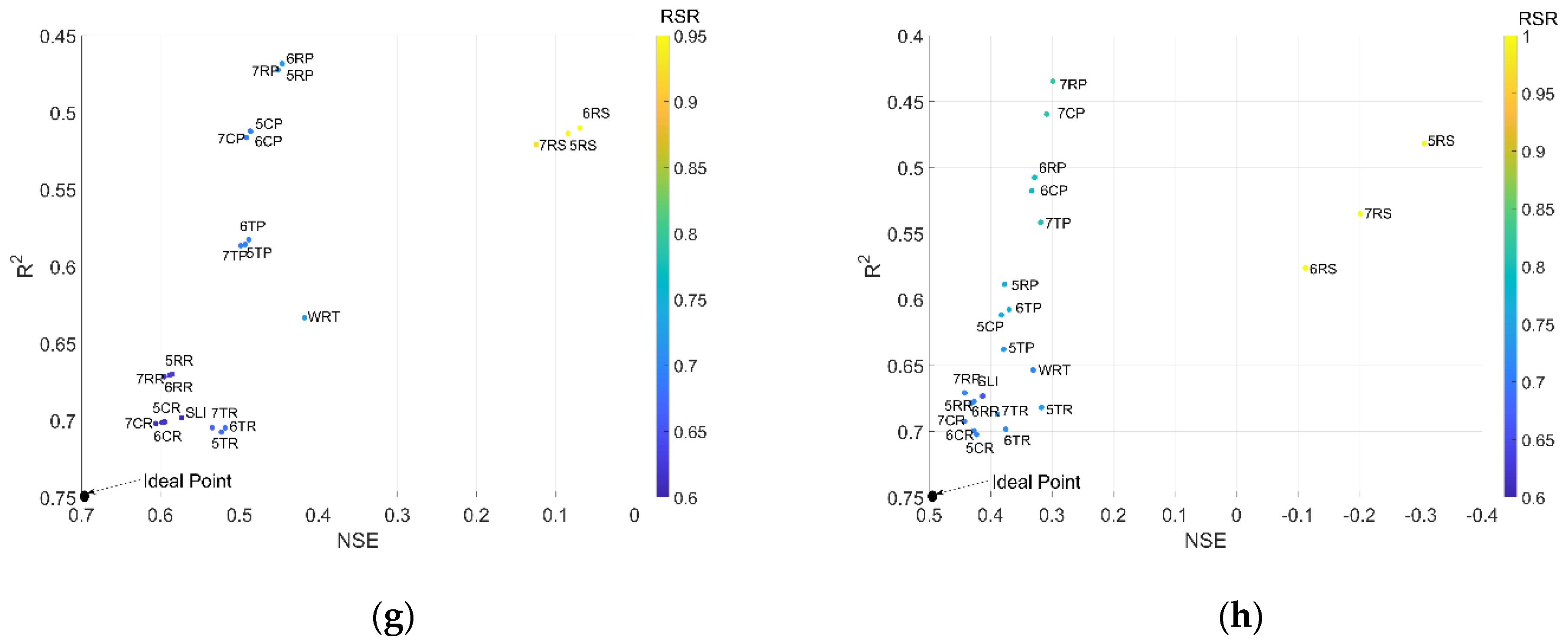
Figure 11.
Evaluation of 23 estimation methods combining three error evaluation methods based on the station: (a) Cuyahoga, (b) Grand, (c) Great Miami, (d) Maumee, (e) Muskingum, (f) Raisin, (g) Sandusky, and (h) Vermilion.
Figure 11.
Evaluation of 23 estimation methods combining three error evaluation methods based on the station: (a) Cuyahoga, (b) Grand, (c) Great Miami, (d) Maumee, (e) Muskingum, (f) Raisin, (g) Sandusky, and (h) Vermilion.
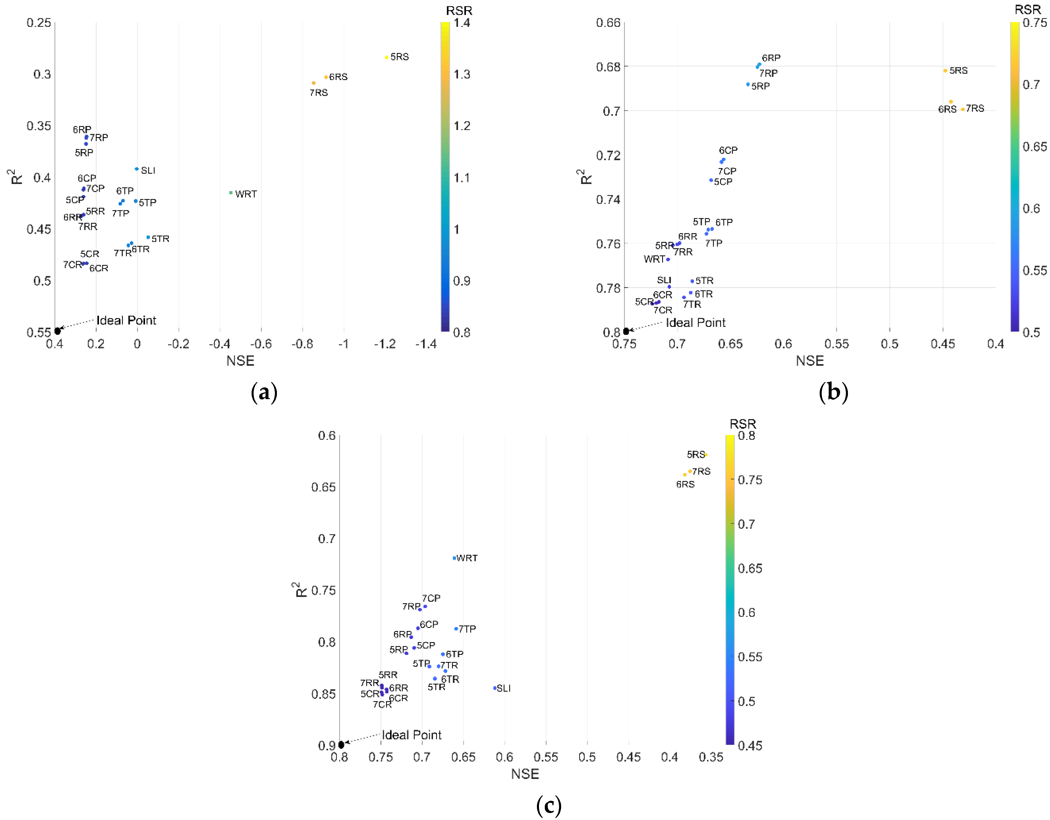
Figure 12.
Evaluation of 23 estimation methods combining three error evaluation methods based on (a) daily concentration, (b) daily load, and (c) annual load.
Figure 12.
Evaluation of 23 estimation methods combining three error evaluation methods based on (a) daily concentration, (b) daily load, and (c) annual load.
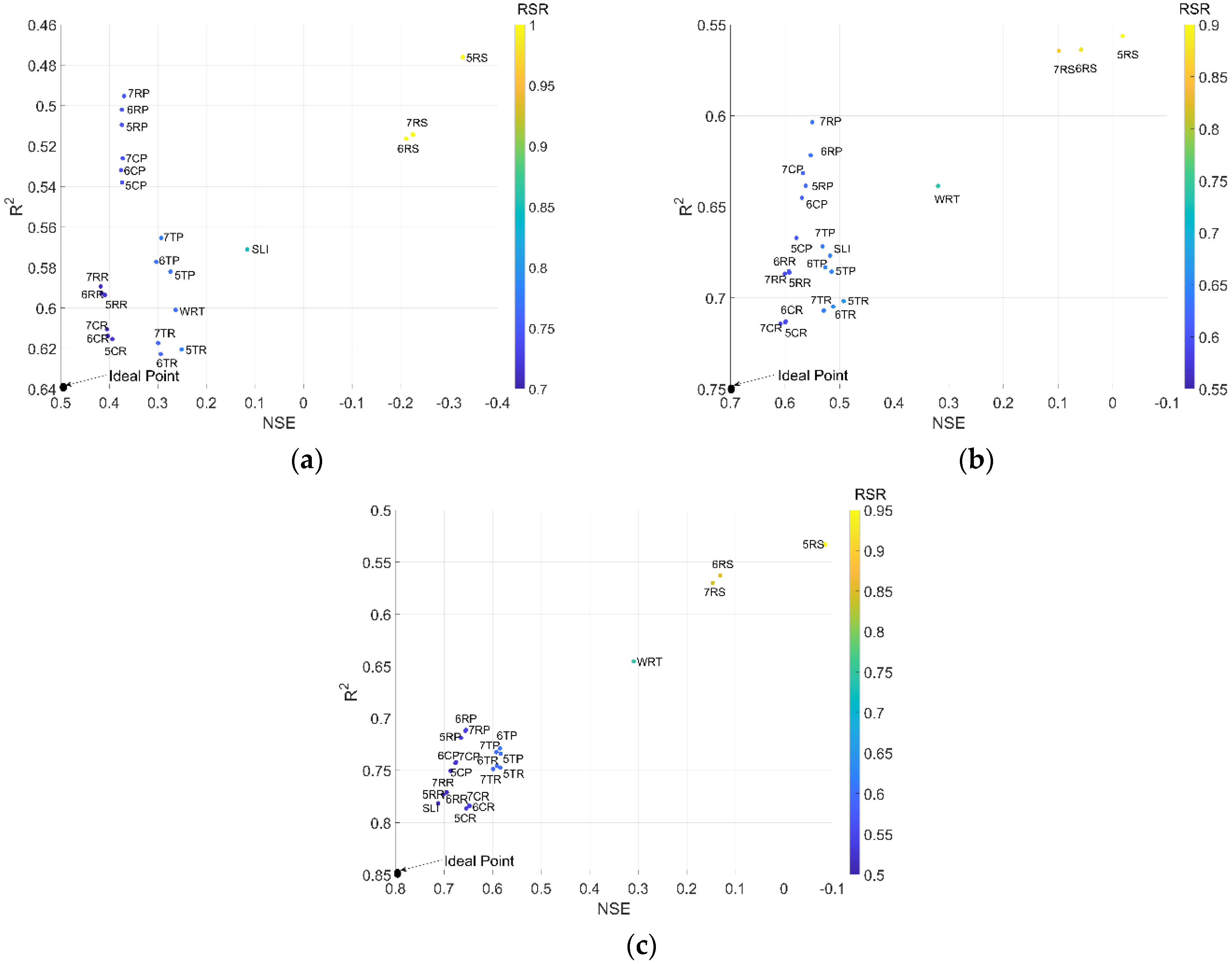
Figure 13.
Evaluation of 23 estimation methods combining three mean error evaluation methods based on sampling frequency: (a) low frequency, (b) medium frequency, and (c) high frequency.
Figure 13.
Evaluation of 23 estimation methods combining three mean error evaluation methods based on sampling frequency: (a) low frequency, (b) medium frequency, and (c) high frequency.
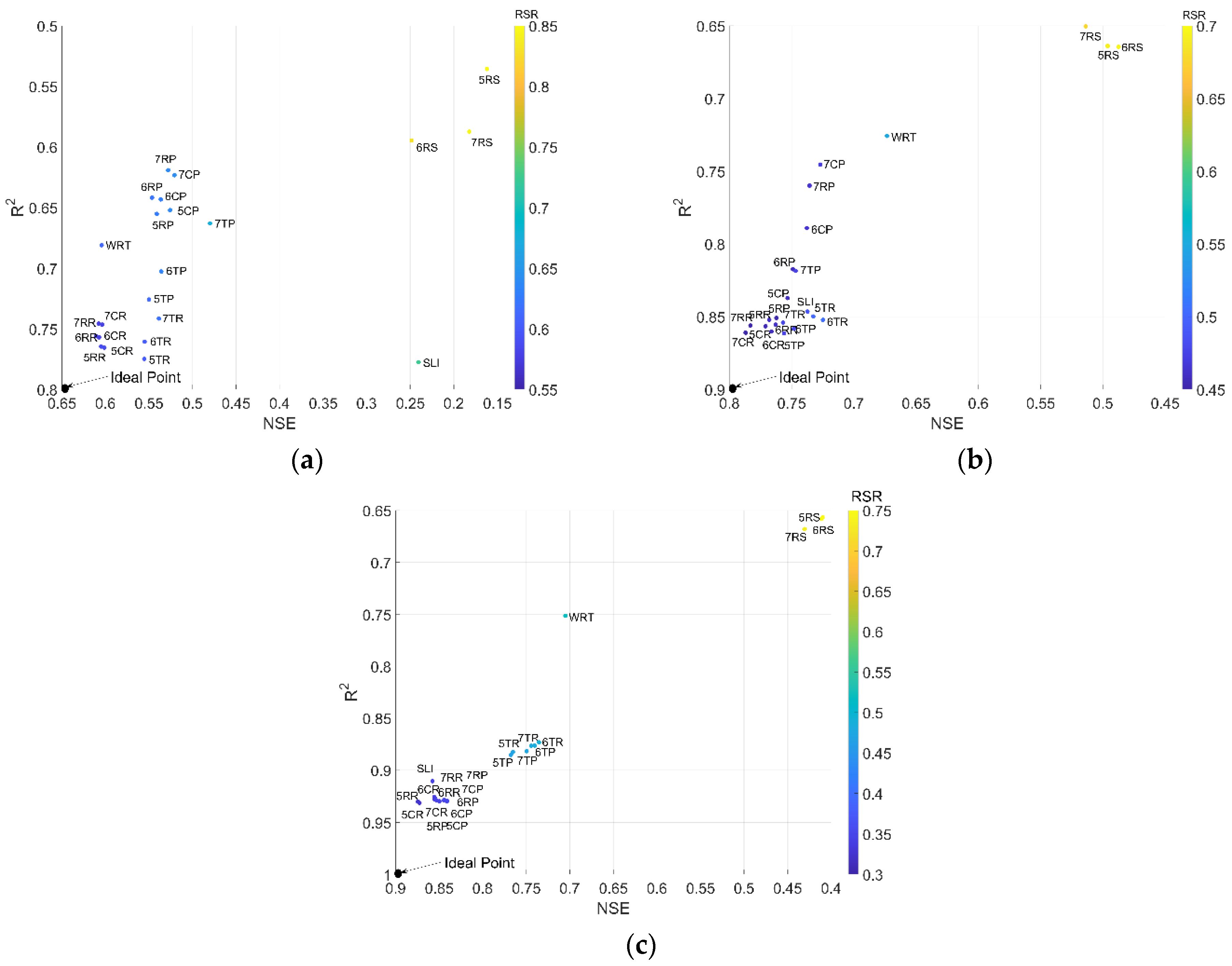
Figure 14.
Evaluation of 23 estimation methods combining three error evaluation methods of mean annual load based on sampling frequency: (a) low frequency, (b) medium frequency, and (c) high frequency.
Figure 14.
Evaluation of 23 estimation methods combining three error evaluation methods of mean annual load based on sampling frequency: (a) low frequency, (b) medium frequency, and (c) high frequency.
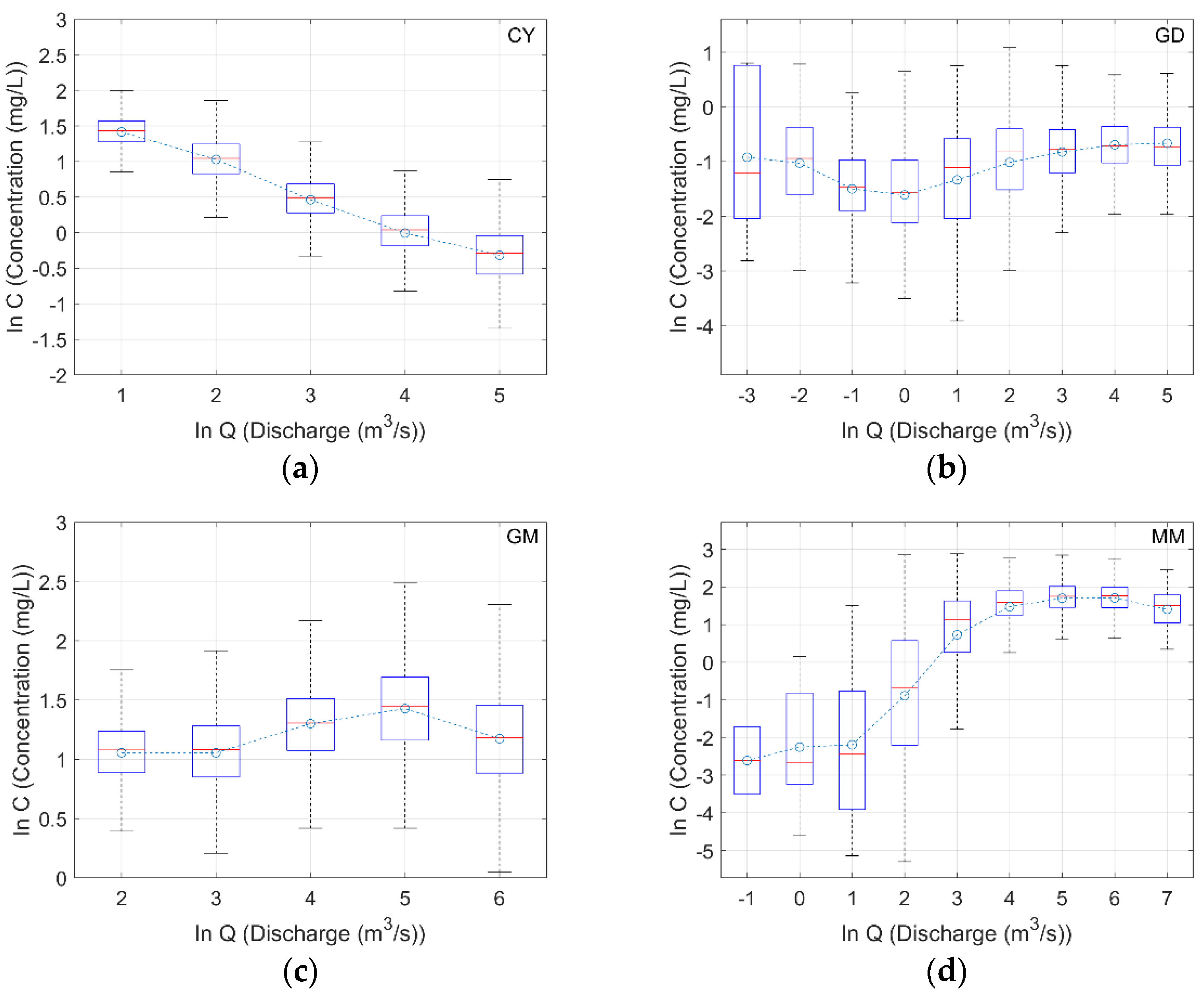
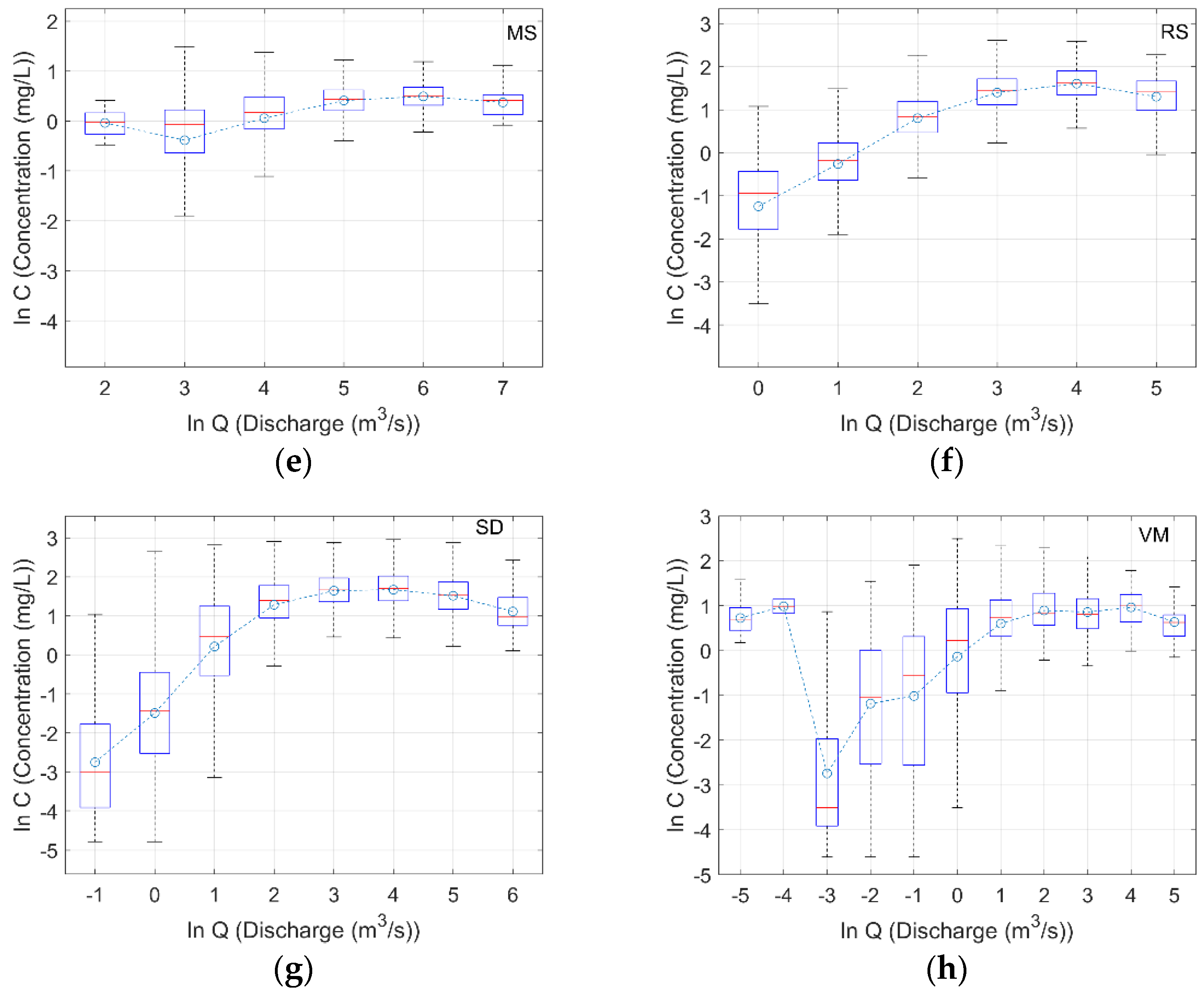
Figure 15.
Observed nitrate box plots based on observed streamflow binning: (a) Cuyahoga, (b) Grand, (c) Great Miami, (d) Maumee, (e) Muskingum, (f) Raisin, (g) Sandusky, and (h) Vermilion (note: circles indicate the mean of binned nitrate concentration).
Figure 15.
Observed nitrate box plots based on observed streamflow binning: (a) Cuyahoga, (b) Grand, (c) Great Miami, (d) Maumee, (e) Muskingum, (f) Raisin, (g) Sandusky, and (h) Vermilion (note: circles indicate the mean of binned nitrate concentration).
Table 1.
Characteristics of applied gaging stations and the corresponding watersheds [
15,
16].
Table 1.
Characteristics of applied gaging stations and the corresponding watersheds [
15,
16].
| | USGS Station Number | Monitoring Period | Watershed Size (km2) | Years Selected | Land Use (%) |
|---|
| Agriculture | Urban | Wooded |
|---|
| Lake Erie basin | | | | | | | |
| Cuyahoga (CY) | 04208000 | 1982–2017 | 1843 | 36 | 17 | 47 | 35 |
| Grand (GD) | 04212100 | 1989–2006 | 1758 | 18 | 37 | 10 | 52 |
| Maumee (MM) | 04193500 | 1975–2017 | 16,427 | 43 | 81 | 11 | 8 |
| Raisin (RS) | 04176500 | 1982–2017 | 2755 | 36 | 72 | 11 | 16 |
| Sandusky (SD) | 04198000 | 1975–2017 | 3285 | 43 | 83 | 9 | 8 |
| Vermilion (VM) | 04199500 | 2001–2008 | 697 | 8 | 71 | 1 | 26 |
| Ohio River basin | | | | | | | |
| Great Miami (GM) | 03271601 | 1996–2017 | 6953 | 22 | 82 | 5 | 10 |
| Muskingum (MS) | 03150000 | 1995–2017 | 19,208 | 23 | 52 | 2 | 43 |
Table 2.
Applied daily concentration, daily load and annual load estimation methods in this study and their symbols.
Table 2.
Applied daily concentration, daily load and annual load estimation methods in this study and their symbols.
| Estimation Methods | Regression (RS) | Composite Residual (CR) | Composite Proportional (CP) | Triangular Residual (TR) | Triangular Proportional (TP) | Rectangular Residual (RR) | Rectangular Proportional (RP) |
|---|
| 5-parameter | 5RS | 5CR | 5CP | 5TR | 5TP | 5RR | 5RP |
| 6-parameter | 6RS | 6CR | 6CP | 6TR | 6TP | 6RR | 6RP |
| 7-parameter | 7RS | 7CR | 7CP | 7TR | 7TP | 7RR | 7RP |
| Simple Linear Interpolation | SLI | | | | | | |
| WRTDS | WRT | | | | | | |
Table 3.
Priority rankings (Equation (15)) of estimation methods based on the combined daily and annual load estimations in each watershed.
Table 3.
Priority rankings (Equation (15)) of estimation methods based on the combined daily and annual load estimations in each watershed.
| Ranking | Cuyahoga (CY) | Grand (GD) | Great Miami (GM) | Maumee (MM) | Muskingum (MS) | Raisin (RS) | Sandusky (SD) | Vermilion (VM) |
|---|
| 1 | WRT | 7CP | 7CP | SLI | 6CR | 7CR | 7CR | SLI |
| 2 | 6CP | 6CP | 6CP | 5CR | 5CR | 6CR | 6CR | 7CR |
| 3 | 7CP | 5CP | 7RP | 6CR | 7CR | 5CR | 5CR | 7RR |
| 4 | 5CP | 7CR | 6RP | 7CR | 7TR | 7RR | SLI | 5CR |
| 5 | 5RP | 6CR | 5CP | 5RR | 7TP | 7CP | 7RR | 6CR |
| 6 | 6RP | 5CR | 7CR | 6RR | 6TR | 6CP | 6RR | 5RR |
| 7 | 7RP | 7RR | 5RP | 7RR | 6TP | 5CP | 5RR | 6RR |
| 8 | 5CR | 6RR | 6CR | 5TP | 6RR | 6RR | 7TR | 7TR |
| 9 | 6CR | 5RR | 7RR | 5TR | 5RR | 5RR | 5TR | 6TR |
| 10 | 5RR | 6RP | 6RR | 7TP | 7RR | 7RP | 6TR | 5TP |
Table 4.
Priority rankings (Equation (15)) of estimation methods based on daily concentration, daily load, and annual load estimations.
Table 4.
Priority rankings (Equation (15)) of estimation methods based on daily concentration, daily load, and annual load estimations.
| Ranking | Daily Concentration | Daily Load | Annual Load |
|---|
| 1 | 7CR | 5CR | 7CR |
| 2 | 6CR | 7CR | 5CR |
| 3 | 7RR | 6CR | 7RR |
| 4 | 5CR | SLI | 5RR |
| 5 | 6RR | EGR | 6CR |
| 6 | 5RR | 5RR | 6RR |
| 7 | 5CP | 7RR | 5RP |
| 8 | 7CP | 7TR | 6RP |
| 9 | 6CP | 6RR | 5CP |
| 10 | 5RP | 6TR | 6CP |
Table 5.
Priority rankings (Equation (15)) of estimation methods combining daily concentration, daily load and annual load estimations with eight stations based on sampling frequency.
Table 5.
Priority rankings (Equation (15)) of estimation methods combining daily concentration, daily load and annual load estimations with eight stations based on sampling frequency.
| Ranking | Low Frequency | Medium Frequency | High Frequency |
|---|
| 1 | 6CR | 7CR | SLI |
| 2 | 7CR | 6CR | 5RR |
| 3 | 5CR | 5CR | 7RR |
| 4 | 6RR | 7RR | 6RR |
| 5 | 7RR | 5RR | 5CR |
| 6 | 5RR | 6RR | 7CR |
| 7 | 6TR | 7TR | 6CR |
| 8 | 7TR | 5CP | 5CP |
| 9 | 5TR | 6TR | 7CP |
| 10 | WRT | 6TP | 6CP |
Table 6.
The priority rankings of estimation methods combining eight stations for annual load depend on sampling frequency.
Table 6.
The priority rankings of estimation methods combining eight stations for annual load depend on sampling frequency.
| Ranking | Low Frequency | Medium Frequency | High Frequency |
|---|
| 1 | 6RR | 7CR | 5RR |
| 2 | 6CR | 7RR | 5CR |
| 3 | 7RR | 5CR | 7CR |
| 4 | 7CR | 5RP | 7RR |
| 5 | 5RR | 6CR | 6RR |
| 6 | 5CR | 5RR | 6CR |
| 7 | 5TR | 6RR | 5RP |
| 8 | 6TR | 5CP | 5CP |
| 9 | WRT | 5TP | SLI |
| 10 | 5TP | 6RP | 7RP |


 ,
, 


