
PV/Wind-Integrated Low-Inertia System Frequency Control: PSO-Optimized Fractional-Order PI-Based SMES Approach


1
K.A.CARE Energy Research & Innovation Center, King Fahd University of Petroleum & Minerals (KFUPM), Dhahran 31261, Saudi Arabia
2
Department of Electrical Engineering, King Fahd University of Petroleum & Minerals (KFUPM), Dhahran 31261, Saudi Arabia
3
Center for Environment & Marine Studies, Research Institute, King Fahd University of Petroleum & Minerals (KFUPM), Dhahran 31261, Saudi Arabia
4
Center for Renewable Energy & Power Systems, King Fahd University of Petroleum & Minerals (KFUPM), Dhahran 31261, Saudi Arabia
*
Author to whom correspondence should be addressed.
Sustainability 2021, 13(14), 7622; https://0-doi-org.brum.beds.ac.uk/10.3390/su13147622
Submission received: 17 May 2021
/
Revised: 20 June 2021
/
Accepted: 25 June 2021
/
Published: 7 July 2021
(This article belongs to the Special Issue Sustainable Energy Systems: Emerging Technologies and Practices in Renewable Energy Storage)
Abstract
:A paradigm shift in power engineering transforms conventional fossil fuel-based power systems gradually into more sustainable and environmentally friendly systems due to more renewable energy source (RES) integration. However, the control structure of high-level RES integrated system becomes complex, and the total system inertia is reduced due to the removal of conventional synchronous generators. Thus, such a system poses serious frequency instabilities due to the high rate of change of frequency (RoCoF). To handle this frequency instability issue, this work proposes an optimized fractional-order proportional integral (FOPI) controller-based superconducting magnetic energy storage (SMES) approach. The proposed FOPI-based SMES technique to support virtual inertia is superior to and more robust than the conventional technique. The FOPI parameters are optimized using the particle swarm optimization (PSO) technique. The SMES is modeled and integrated into the optimally designed FOPI to support the virtual inertia of the system. Fluctuating RESs are considered to show the effectiveness of the proposed approach. Extensive time-domain simulations were carried out in MATLAB Simulink with different load and generation mismatch levels. Systems with different inertia levels were simulated to guarantee the frequency stability of the system with the proposed FOPI-based SMES control technique. Several performance indices, such as overshoot, undershoot, and settling time, were considered in the analysis.
1. Introduction
Due to the continuous depletion of fossil fuels, increased government incentives, technological advancements, and price drops, the utilization of renewable energy sources (RESs) as distributed generators (DGs) has increased dramatically in recent years. In power systems, several technical issues, such as low reserve generation, fault ride through capability, inertia, and high fault current, have arisen because of high-level RES integration [1]. Thus, the frequency stability issue of high-level RES-integrated systems is greatly affected. Moreover, the two main sources of renewable energy, solar and wind, are highly unpredictable. The intermittent and unpredictable RESs can be modeled with sophisticated methods to lower the risk of instability in power systems [2]. A high share of RESs complicates grid-balancing and market operations. Several dedicated devices can be installed in a RES-integrated system to provide ancillary services such as power variations, congestion reduction, grid balancing, and primary reserve [3,4]. The technical issues of RES integration with a power system could also be handled with different cutting edge technologies such as modern control and optimization techniques, energy storage devices including batteries and supercapacitors, and fault current limiting devices [5].
The overall inertia of a power system is decreased greatly as a result of the integration of low-inertia wind and inertia-less PV systems [6]. Power electronic converter decoupling between the wind generator and the power system is responsible for the low inertia. As a result, such a low-inertia wind system cannot properly maintain the frequency stability of the power system. Moreover, solar PV with no inertia is highly responsible for the frequency deviation of the system. Therefore, high-level PV and wind penetration reduces the total inertia and augments the rate of change of frequency (RoCoF), which are responsible for the unexpected load-shedding controller activation even at small generation–load mismatch [7]. In addition, reserve power reduction due to high-level PV/wind integration causes frequency deviation [8]. In summary, inertia emulation controllers need to be designed to improve the frequency stability of RES-integrated power systems.
In order to minimize the frequency excursion of a low-inertia system, several methods have been presented in the literature, such as the auxiliary load frequency (LFC) control technique, the inertia emulation technique, the deloading technique, the droop technique, and the energy storage-based technique [9,10,11,12]. In [13], an auxiliary LFC technique was presented to control the frequency of the Egyptian grid considering high-level PV and wind integration employing the proportional-integral-derivative (PID) controller. However, the LFC technique does not consider the detailed model of the Egyptian grid; instead, it excludes tie line power flow, which needs further investigation. In general, conventional PI and PID controllers, the parameters of which were fine-tuned experimentally or tuned by Ziegler–Nichols methods, were employed in system frequency control [14,15]. However, the conventional tuning methods of PI/PID controllers may not provide satisfactory performance. In [16], a virtual inertia support technique was presented for a low-inertia microgrid with a particle swarm optimization (PSO)-based PI controller.
The superconducting magnetic energy storage (SMES) is considered a promising device for the low-inertia issue of the microgrid system in [17]. The conventional derivative approach for the virtual inertia control loop was implemented. The detailed design of feedback and proportion gains, however, were not discussed in this work. Another energy storage, the battery, was presented in [18] for frequency support of the doubly fed induction generator (DFIG)-based wind system. The battery was connected to the DC link of DFIG and controlled with the droop technique in order to reduce frequency deviation by scheduling active power exchange during system disturbances. In [19], a self-adaptive virtual inertia fuzzy controller was adopted for a high-level renewable integrated system. The proportional virtual gain was adapted by the fuzzy system, which uses the deviation of real power and frequency as it inputs. In this scheme, however, the generalized energy storage system (ESS) was considered a simple first-order system. Since the specific ESS was neither discussed nor modeled, the presented frequency support scheme needs further improvement or investigation. The sharing of active power from different energy storage devices were scheduled based on their abilities in [20] for frequency control of renewable sources. In this capability-coordinated frequency control (CCFC) approach, the total error signal was forwarded to the primary control loop of each unit based on its capabilities. The LFC for mass-less inertia PV systems was presented in [21] with PI controllers. The parameters were optimized with the hybrid optimization technique in the case of different step load changes. In order to stabilize the low-inertia PV system, another virtual inertia synthetization using a synchronverter was reported in [22] with the learning technique. The optimized virtual inertia frequency control and protection schemes were developed in [23,24] for a low-frequency interconnected power system. The combination of SMES and thyristor-controlled phase shifters (TCPS) [25] was applied in a low-inertia utility grid with the adaptive neuro-fuzzy system (ANFIS) controller. The detailed design of SMES negative feedback and proportional gains, however, was not considered. The main advantage of SMES is the quick charging/discharging ability to react to sudden changes in system dynamics. Thus, the fast-response capability of SMES could be the most effective countermeasure against frequency deviations in a power system. The voltage and frequency stability issues of a power system are addressed in some of the literature with SMES [26,27,28]. Furthermore, the transient stability issues are also handled with the application of SMES [29,30,31]. Based on a comprehensive literature survey on SMES device applications in power systems, it is concluded that further study on virtual inertia control topologies using SMES is imperative.
In recent years, several theoretical and applied studies have been conducted on fractional-order controllers [32,33]. Better system performance is observed with fractional-order controllers over conventional PI controllers because the fractional-order controller involves additional real parameters [34]. However, in general, there is no hard and fast rule for tuning the parameters of fractional-order controllers. The tuning of fractional-order proportional integral (FOPI) controller parameters with the artificial bee colony (ABC) [35] technique has been presented, which is complex in objective function evaluation and low convergence speed. The parameter-tuning task of FOPI is formulated as an optimization problem and solved with the seeker optimization algorithm (SOA) in [36]. The harmony search (HS) algorithm is reported in [37] for FOPI parameter optimization to control the power-switched reluctance motor. However, there are no conclusive studies on the application of the virtual inertia technique using an SMES topology-based FOPI controller.
Based on several studies [17,18,19,25,38], it is identified that the detailed design of the PSO-optimized SMES is missing the FOPI controller to support virtual inertia for RESs. Thus, in this paper, we propose a PSO-optimized FOPI-SMES controller design approach for a two-area power system. The proposed approach can support the virtual inertia of the high-level renewable energy integrated system. The addition of this virtual inertia makes the system stable over a wide range of load–generation mismatches. Since the FOPI controller is superior to the conventional PI, the proposed technique performs better when reducing system frequency deviation. However, the design of FOPI is challenging compared to the conventional PI. Thus, this work introduces a detailed model of FOPI, SMES, and a two-area power system to find the design parameters. The dynamic model of the system presented along with SMES and FOPI is utilized to develop the frequency deviation-based cost function for the PSO algorithm. To validate the proposed optimized FOPI controller-based SMES, several case studies were considered and simulated for a wide range of load profile variations. The robustness of the proposed virtual inertia control scheme was tested under reduced system inertia. The proposed controller was compared with the conventional controller, where the improvements in several indices, such as total frequency deviation, overshoot, undershoot, and settling time, were observed. Furthermore, the performance of the non-optimized FOPI was compared with the PSO-optimized FOPI.
The manuscript is organized as follows. The dynamic model of the system including RESs is given in Section 2. The SMES modeling and PSO-based FOPI-SMES design techniques are discussed in Section 3. The simulation results are discussed in Section 4. Finally, the conclusions of this study are given in Section 5.
2. High-Level PV/Wind-Integrated System Modeling
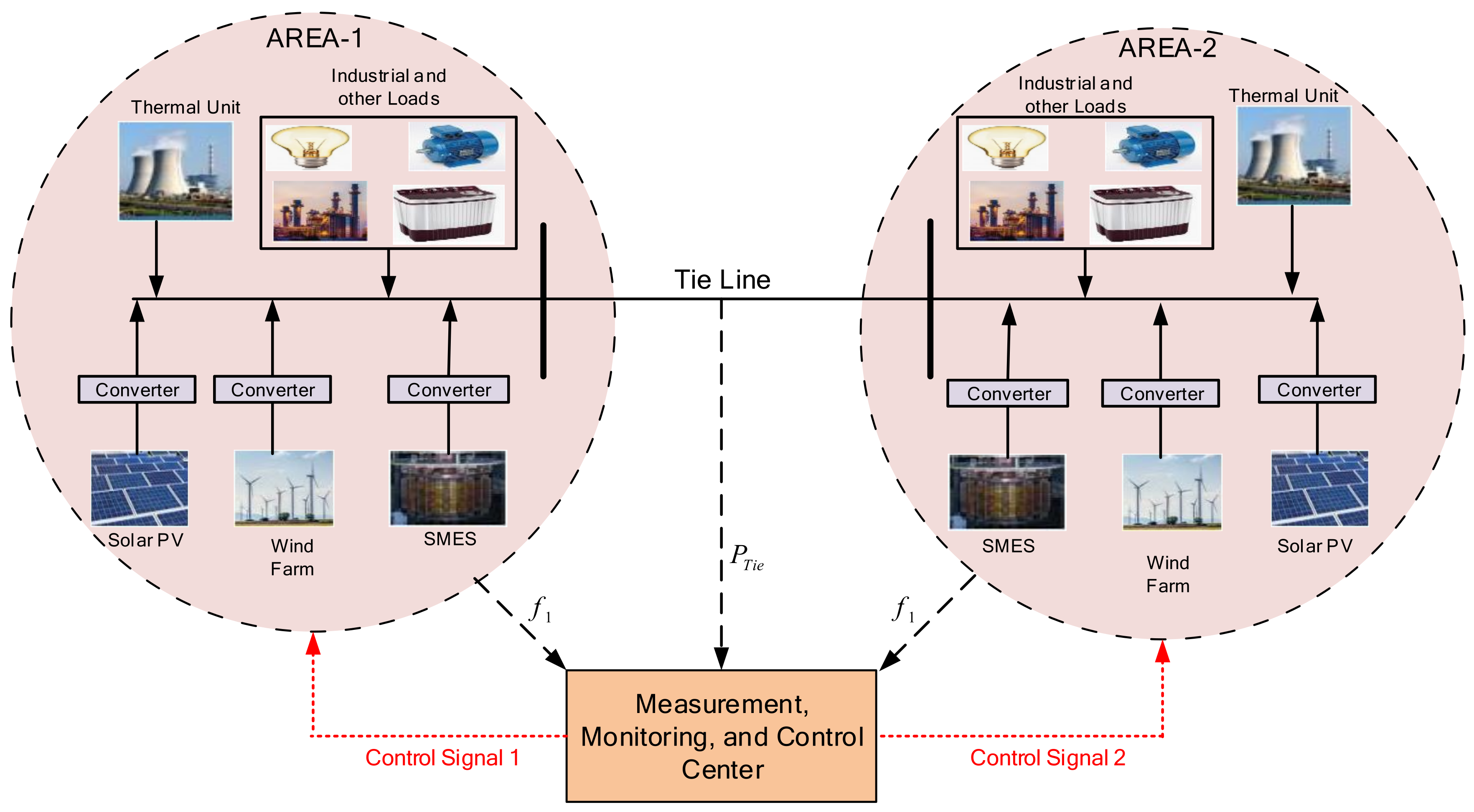
The fractional-order PI controller for superconducting magnetic energy storage (SMES) is designed to virtually support inertia for a high-level solar PV- and wind-integrated two-area power system. An interconnected power system with low inertia due to a high-level integration of PV and wind energy sources, as shown in Figure 1, is considered in this study. The areas are connected by a tie-line, and both of them consist of thermal generating units, an industrial load, a residential load, solar PV, wind, and SMES. The measured frequency and tie-line signals are accumulated in the control and monitoring center. Since the system faces low inertia, it is expected to support the inertia via the control center, which sends control signals to the controllable energy storage devices of both areas if the communication network is available. However, in absence of a communication link, local controllers such as decentralized control, primary control, and droop control can be employed. The net power () in each area in Figure 1 can be calculated using the power of (1) the thermal unit (), (2) the solar array (), (3) the wind farm (), (4) SMES (), (5) combined industrial and other loads (), and (6) the tie-line (). The expression for is given below.
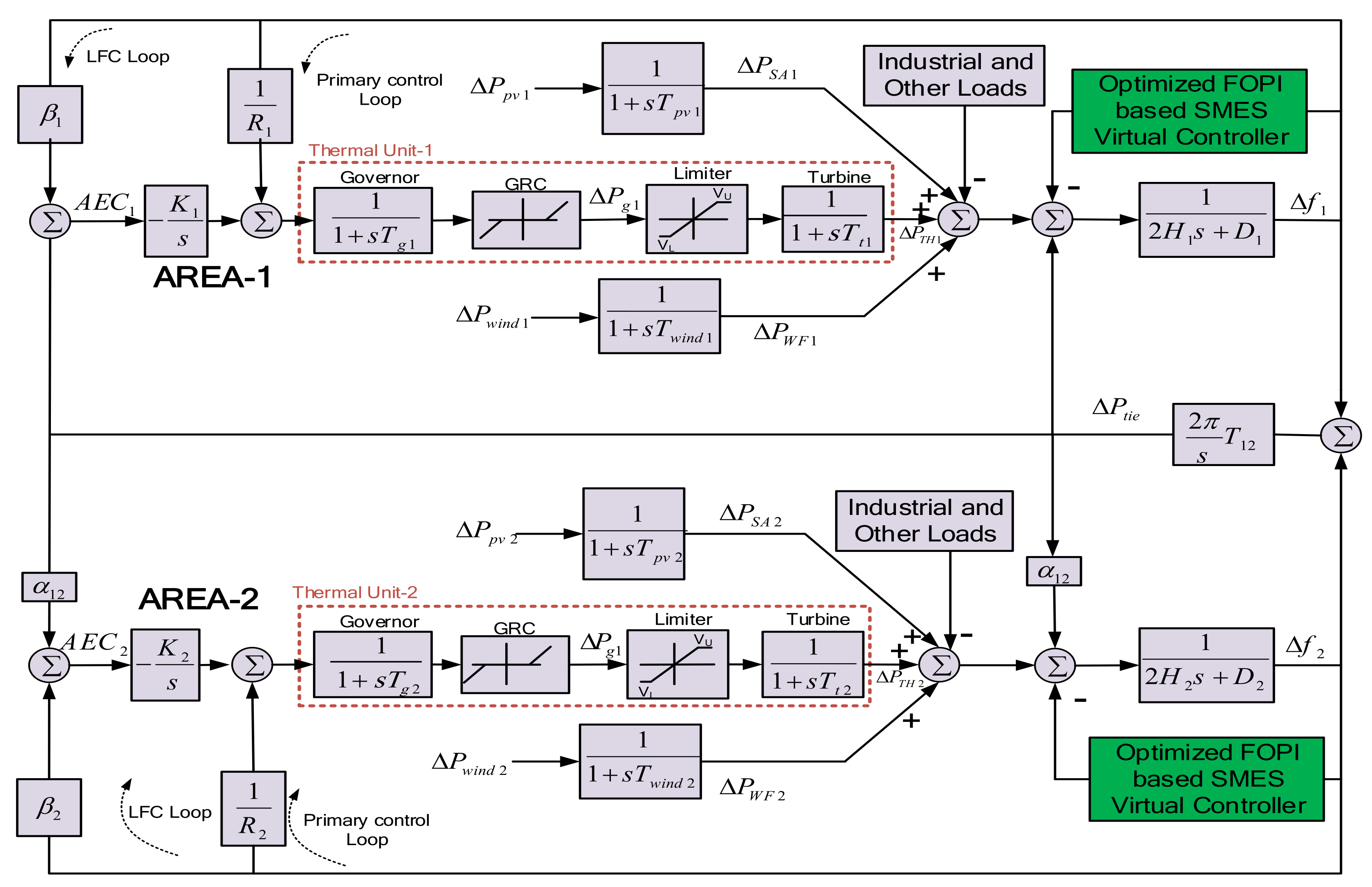
In general, higher-order models for thermal generating units, wind systems, solar PV, and converters, with nonlinearity are considered to precisely demonstrate the dynamic behaviors of the interconnected system. For large power systems with power electronic converters, however, simplified dynamic models are employed to study the frequency stability. The interested readers can find more details on such dynamic modeling in [39,40,41]. The simplified dynamic model of the two-area system can be developed as shown in Figure 2 for frequency stability analysis.
From the dynamic model, as shown in Figure 2, the frequency deviation for the kth area can be written as follows.
where,
where is the inertia constant in area k, is the damping constant in area k, is the incremental power of the thermal unit in area k, is the incremental power of solar farm in area k, is the incremental power of wind farm in area k, is the turbine time constant in area k, is the governor time constant in area k, is the wind turbine time constant in area k, and is the solar system time constant in area k.
Two physical constraints, governor dead band (GDB) and generation rate constraint (GRC), affect the dynamic performance of the power system. The thermal units consist of rotating mass, which inherentlyhas mechanical inertia; thus, it puts a constraint/limit on the output power change, which is known as GRC. The controller designed without GRC may not perform well in practical applications. To handle this issue, GRC is considered for the virtual inertia controller design in this work, as shown in Figure 2. Furthermore, the governor cannot change its valve position within a specific range of speed variation. Due to this dead-band, the tie-line power oscillation with a natural frequency of 0.5 Hz is observed. The dead-band for governor is also taken into consideration in this study to reflect the practical implementation case. The solar PV, wind, and different loads are modeled as disturbances in the dynamic model. The interested readers are directed to the literature [39] for more details on dynamic modeling of PV/wind integrated system.
3. SMES Model with FOPI Controller
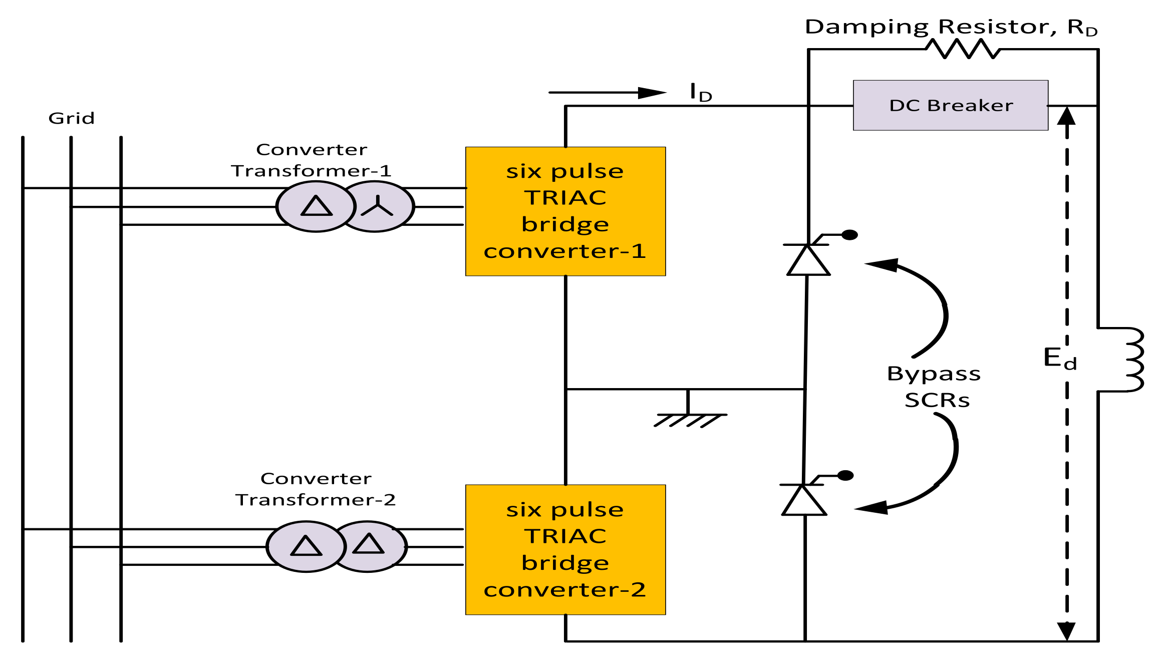
SMES is a promising device for dynamic stability improvement of power systems. The SMES has several components: thte power conversion system (PCS), consisting of the inverter/rectifier, and the superconducting coil which is kept under extremely low temperature [25]. The PCS also consists of three-phase transformers to allow for energy exchange between the AC grid and the superconducting coil. The harmonic contents of the signals are filtered by two cascaded six pulse bridges, as shown in Figure 3. The capability of SMES to exchange huge power within a very short duration has drawn the attention of researchers in the power system application.
In normal conditions, the SMES coil charges quickly to its pre-defined peak value. As the coil temperature is maintained below the critical value, it conducts the current with nearly zero loss. During contingencies, as the power demand is initiated by the power system, the SMES discharges power through the PCS to the grid almost instantly. While the governors of the generators support the power demand after contingencies, the SMES again charges at its preset value. The inductor DC voltage is given by the equation below [25,42].
where is the maximum voltage of the bridge circuit, is the triac firing angle, is the superconducting coil current, and is the damping resistor. Thus, the DC voltage appearing across the superconducting coil can be controlled with the variation of the triac firing angle . If is above , the energy stored in the superconducting coil is released to the grid. In contrast, the superconducting coil charges if is below the . In this way, the superconducting coil charges and discharges through the bidirectional converter system to absorb or provide energy.
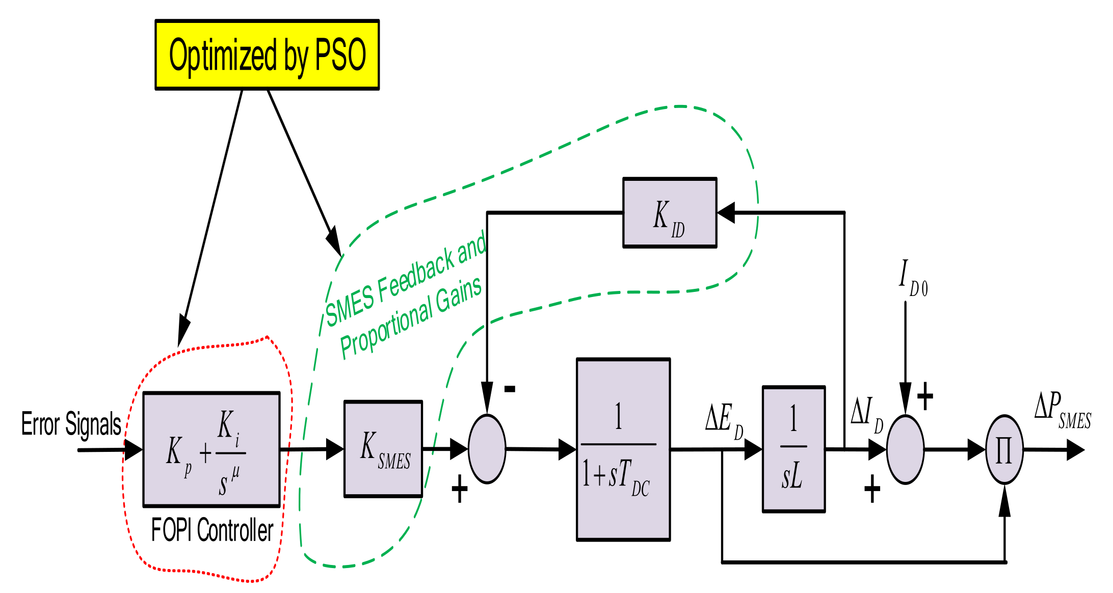
The detailed dynamic model of SMES for frequency stability studies along with the FOPI controller are shown in Figure 4. During excessive system loading, the load surpasses the generation, the becomes negative, while the current maintains the same direction. The incremental change in is written as
where is the SMES gain, is the output of the FOPI controller, is the negative feedback gain, is the incremental change in superconducting coil current, and is the converter delay time. The incremental change in inductor current is written as
3.1. Controller Design
This study focuses on the optimal FOPI-SMES design based on the PSO algorithm to augment the frequency stability of the two-area power system. The fractional-order calculus involves generalized differentiation and integration of non-integer order [33,34]. The fractional-order controller is applied in several engineering fields such as automatic control and power systems due to its superiority over conventional integer order controllers.
The time domain FOPI controller can be represented as
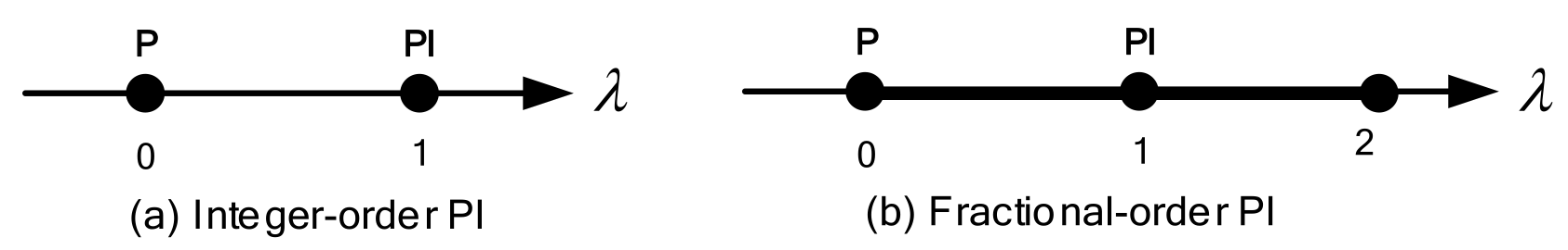
where is the error signal, is the proportional gain, is the integral gain, and is a fractional order and real number that lies between 0 and 2. The Laplace transformation gives the following transfer function for the FOPI controller.
The conventional integer order PI and the FOPI can be understood using Figure 5 in the axis. The integer order controller is represented by two points on the axis. However, the FOPI controller can be represented by the infinite number of points between 0 and 2. Thus, it gives more degree of freedom and flexibility over the conventional integer order controller.
As presented in Figure 4, the SMES virtual inertia based on FOPI is developed in this study to support the frequency of the low-inertia interconnected system. The feedback and proportional gains of SMES along with the FOPI’s proportional gain, integral gain, and fractional parameter are optimized with PSO. The following subsections describe the objective function formulation and solution system with the PSO.
3.2. Description of Cost Function
The appropriate cost function is vital in the application of nature-inspired and heuristic optimization techniques in power systems. In general, the cost function is defined to minimize or maximize some variables. In this work, several FOPI gains, fractional orders, SMES feedback gains, and proportional gains are designed based on tie-line power fluctuation and area frequency deviation. For better comprehension of the optimization process, the following cost function is considered.
where subscripts 1 and 2 are to denote area 1 and area 2 for the interconnected power system. T is the simulation time, is the frequency deviation, is tie-line power deviation, is the FOPI proportional gain, is the FOPI integral gain, is the SMES negative feedback gain, and is the SMES proportional gain. Mainly, the upper and lower limits of Equation (15) are selected based on knowledge/experience of FOPI and SMES applications in power system. The optimization algorithm is coded in a MATLAB script (.m files) environment and linked with the MATLAB Simulink (.slx files) environment.
3.3. Solution Approach with PSO
This study proposes a FOPI-based SMES virtual inertia approach in which the minimization problem described by Equation (13) is solved by the PSO. PSO, a heuristic optimization technique, was inspired by the sociological behavior of birds flocking [43]. In the PSO algorithm, several random particles that move in a search space to find the best minimum or maximum value of the cost function based on the minimization or maximization problem, respectively, are initially generated. The PSO shows outstanding performance compared to the other algorithms, as follows [44,45,46]:
- Since the PSO uses a numerical valued cost function, it is suitable for any nonderivative cost function optimization.
- The PSO facilitates more flexible and robust control frameworks as it uses probability rules.
- It does not fall into premature convergence.
- It has great flexibility for use in online optimization.
- It requires less time compared to other algorithms.
- It provides accurate results with very simple operations.
In recent years, the PSO has been implemented successfully to solve several power system problems such as that presented in [47,48]. The position and velocity vectors in a multi-dimensional solution space for PSO algorithm are mainly described by two equations as follows [49]:
where and are the velocities of ith particle for the kth iteration in a multi-dimension search space and the position of ith particle for the kth iteration in a multi-dimension search space, respectively; and are the individual best and global best, respectively, for the ith particle of the th iteration; and are the uniformly distributed random numbers in [0 1]; and and are the learning factors used to obtain the best solution. In addition, the c is the constriction factor that is calculated from the values of and , as follows:
The maximum velocity and minimum velocity of each particle can be calculated as follows:
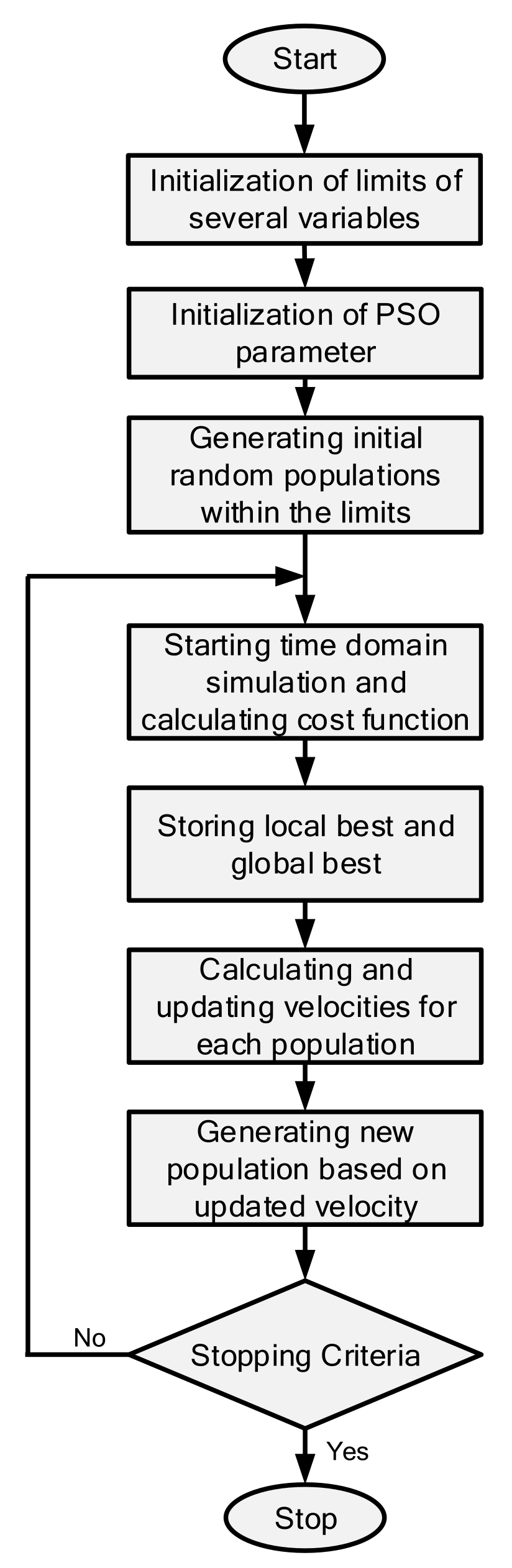
where and are the maximum and minimum velocities of the ith particle, respectively; and are the maximum and minimum limits of the ith particle, respectively; and N is a number that takes a value between 5–10. The PSO solution steps for solving the optimization problem formulated in Section 3.2 is described below.
- Step 2: Selection of the PSO initial parameters including , , maximum iteration, population size, etc.
- Step 3: Generation of the initial population within the limits.
- Step 4: Running the time domain simulation and determining the value of the objective function described by Equation (13).
- Step 5: Storing the local best, the best of the current population, and the global best, the best of the total population.
- Step 6: Updating the velocity of all populations using Equation (16).
- Step 7: Generating a new population based on the updated particle position calculated by Equation (17).
- Step 8: Stopping the optimization if the termination criteria are met. Otherwise, returning to step 4.
The overall flowchart for the PSO algorithm to design FOPI and SMES parameters is shown in Figure 6.
4. Results and Discussion
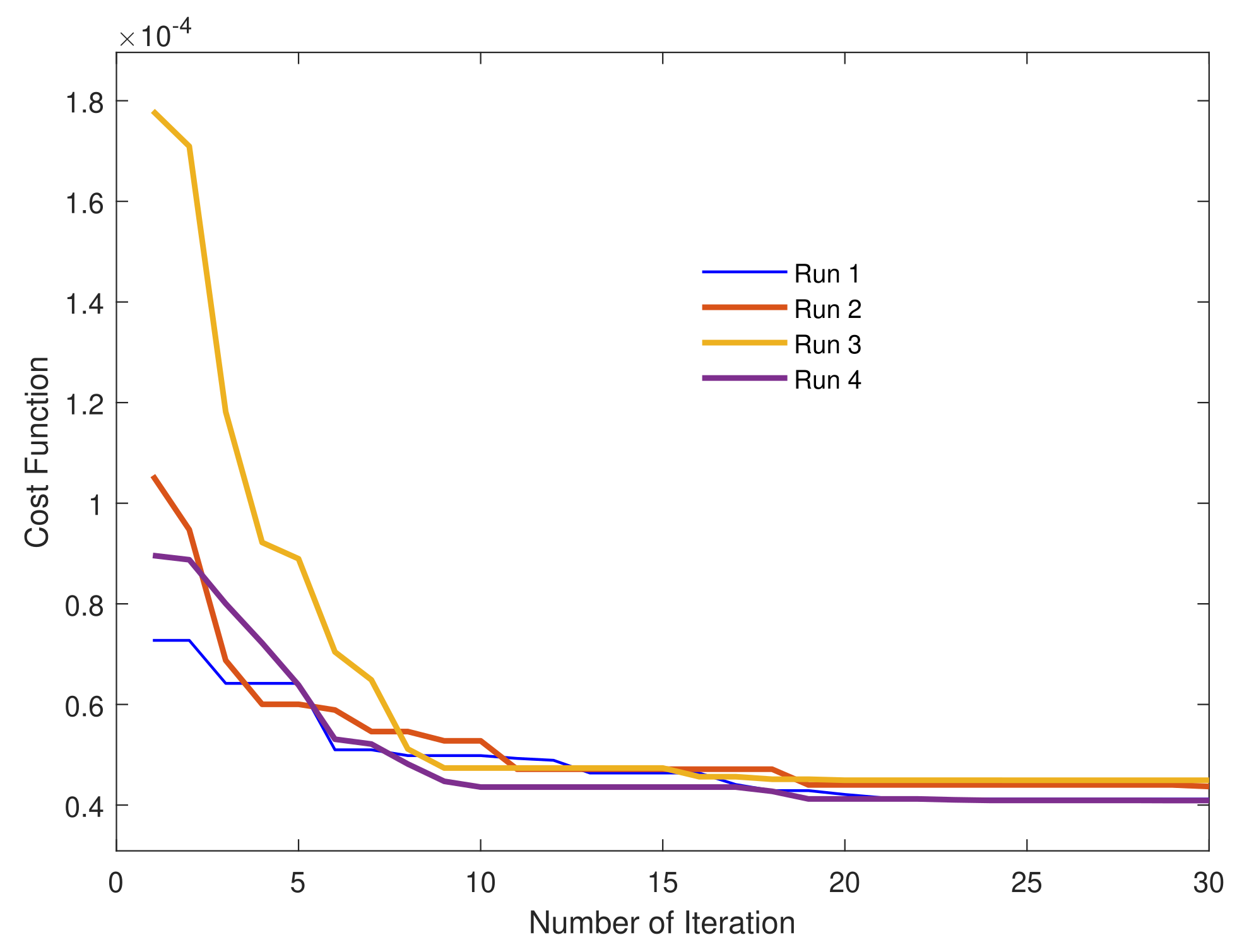
The effectiveness and robustness of the proposed optimized FOPI controller in improving the frequency stability are presented in this section. The dynamic model of the system presented in Figure 2 is considered for analytical analysis. The system parameters listed in Table 1 are used to conduct computer simulations and to facilitate analyses. The total generation capacity of the two-area power is 55 MW. The rating of the energy storage device is 6 MW. The proposed energy storage with only 10.9% of the total plant capacity is capable of maintaining frequency stability in case of several load–generation mismatches. The simulations were conducted in MATLAB Simulink considering several scenarios such as light loading, medium loading, heavy loading, and reduced inertia. The system dynamic model was built in Simulink and linked with the PSO optimization code to optimally design the SMES and FOPI parameters. PSO algorithm convergence for the proposed cost function is depicted in Figure 7. As shown in Figure 7, the optimization algorithm converges at the iteration number 20 for several runs, and the corresponding optimized parameters are listed in Table 2.
The system was tested under several step load variations in both areas of the system. The frequency deviations in both areas were plotted for three cases such as (i) without any inertia controller, (ii) with a conventional SMES controller, and (iii) with the PSO optimized FOPI-based SMES controller.
4.1. Frequency Response Study for Step Load Change in Area 1
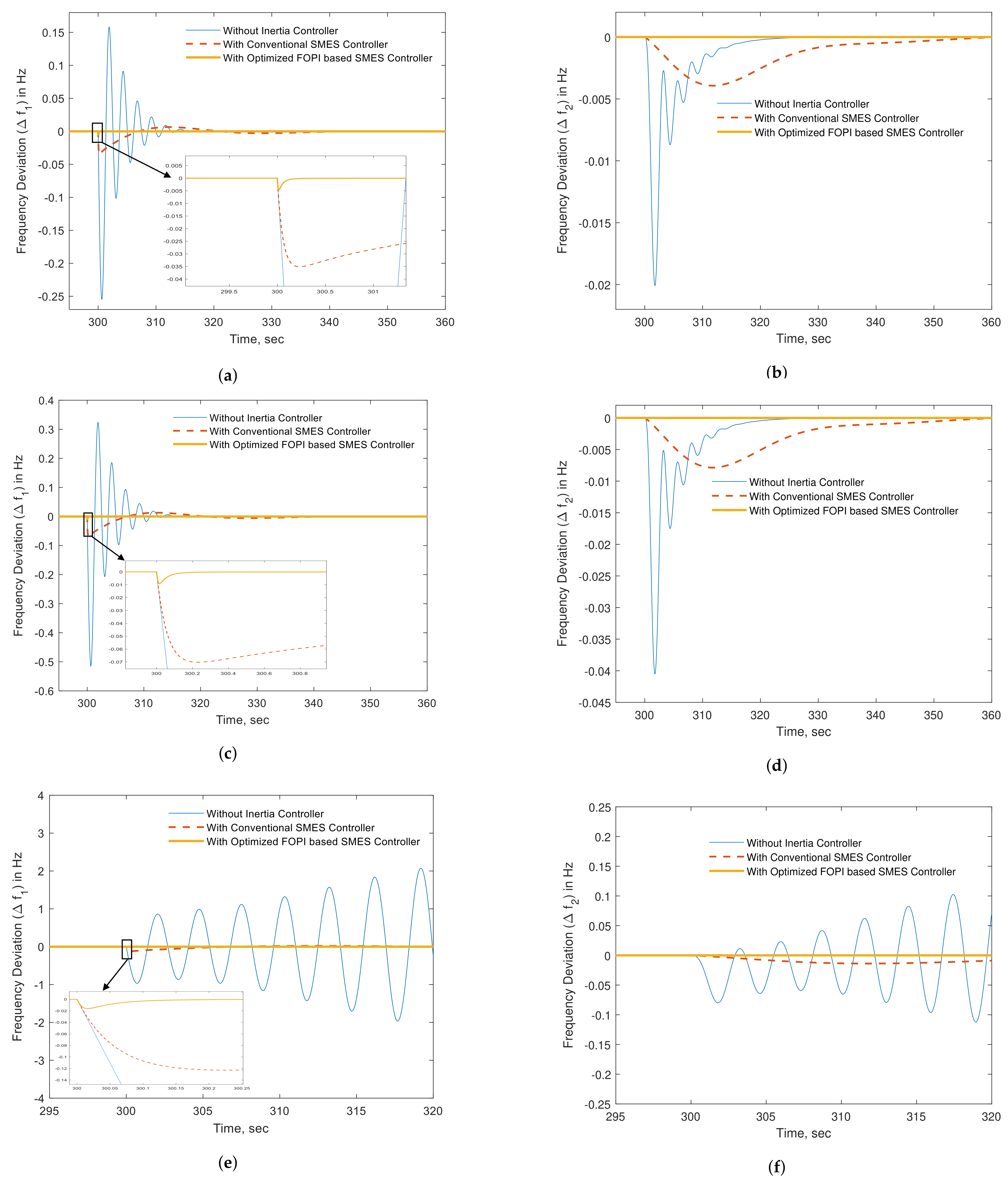
In this case, the studied system is simulated for default inertia (100%), as shown in Table 1. The frequency deviations for both areas are depicted in Figure 8 for low, medium, and high step load changes in area 1. The positive effect of the proposed controller is visualized through the reduction in frequency deviations. As visualized in Figure 8a, a step load change of 0.1 p.u. in area 1 causes a significant frequency deviation in area 1 without a virtual inertia controller. The frequency deviation is around Hz without any auxiliary controller. The conventional controller-based SMES improves the deviation to about Hz. However, the proposed PSO optimization-based FOPI controller for SMES greatly improves the frequency deviation in area 1, which is around Hz. It is noteworthy that the settling time is slightly increased for conventional SMES controllers while the frequency deviation is improved. However, the proposed optimized FOPI-based SMES significantly improves all indices, such as settling time, maximum undershoot, and maximum overshoot. Likewise, the frequency deviation in area 2 is very high, around Hz, without any inertia controller, as depicted in Figure 8b. The conventional SMES controller improves frequency deviation to some extent. However, the proposed optimized FOPI-based SMES controller reduces the frequency deviation to almost zero. It is observed that, for a large step load change (0.35 p.u.) in area 1, the system cannot maintain stable operation. As visualized in Figure 8e,f, the frequency deviations in both areas continue to increase, leading to instability in the system. The application of the conventional SMES controller can maintain stable operation with some frequency deviation. On the other hand, our proposed techniques stabilize the system with almost zero frequency deviations in both areas. Thus, the system response for several load disturbances in area 1 using the proposed controller is faster, has a very small steady-state error, and is better in terms of overshoot and undershoot compared to other control strategies. The frequency deviations for several scenarios in area 1 and area 2 are given in Table 3 to clearly show the positive impact of the proposed FOPI-based SMES controller on system performance.
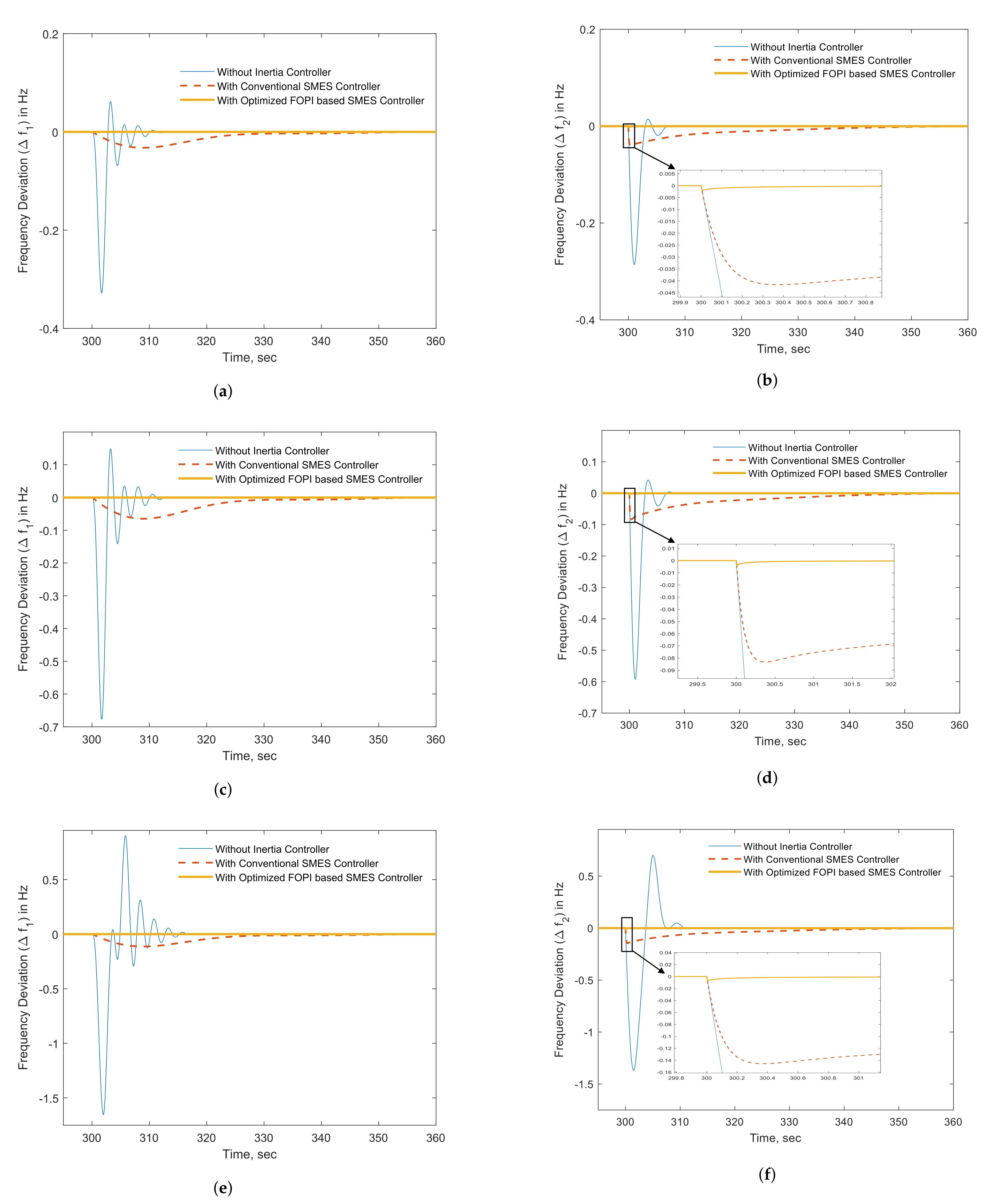
4.2. Frequency Response Study for Step Load Change in Area 2
The load disturbances, ranging from the low to high levels, are also applied in area 2 with the system default inertia. It is noticed that the system frequency oscillates over a wide range without any inertia controller. In some cases, the oscillations are beyond the acceptable limits; thus, it requires the system frequency protection relay to operate. As depicted in Figure 9, the frequency deviation in area 1 is Hz without any virtual inertia controller for a step load change of 0.1 p.u. The conventional SMES controller reduces the frequency deviation to Hz, whereas the proposed optimized FOPI controller is capable of maintaining almost zero frequency deviation. Similarly, the frequency deviation in area 2 is Hz without any auxiliary controller. The conventional SMES controller is capable of reducing the frequency deviation by 90.6%. However, the proposed optimized FOPI-based SMES controller reduces the frequency deviation by 96.87%. For the medium and high step load changes in area 2, at 0.2 p.u. and 0.35 p.u., respectively, the frequencies of both areas fall below the under-frequency relay operating setpoint of 59.5 Hz [50] without any virtual inertia controller.
However, the frequency deviation is well below the under-frequency relay operating point with the conventional SMES controller, as depicted in Figure 9c–f. In these figures, it is visualized that the proposed controller is capable of maintaining the frequency deviations in both areas at almost zero. Thus, the system stability and reliability are guaranteed with the proposed FOPI-based SMES controller. The overall frequency deviations for several cases are listed in Table 3.
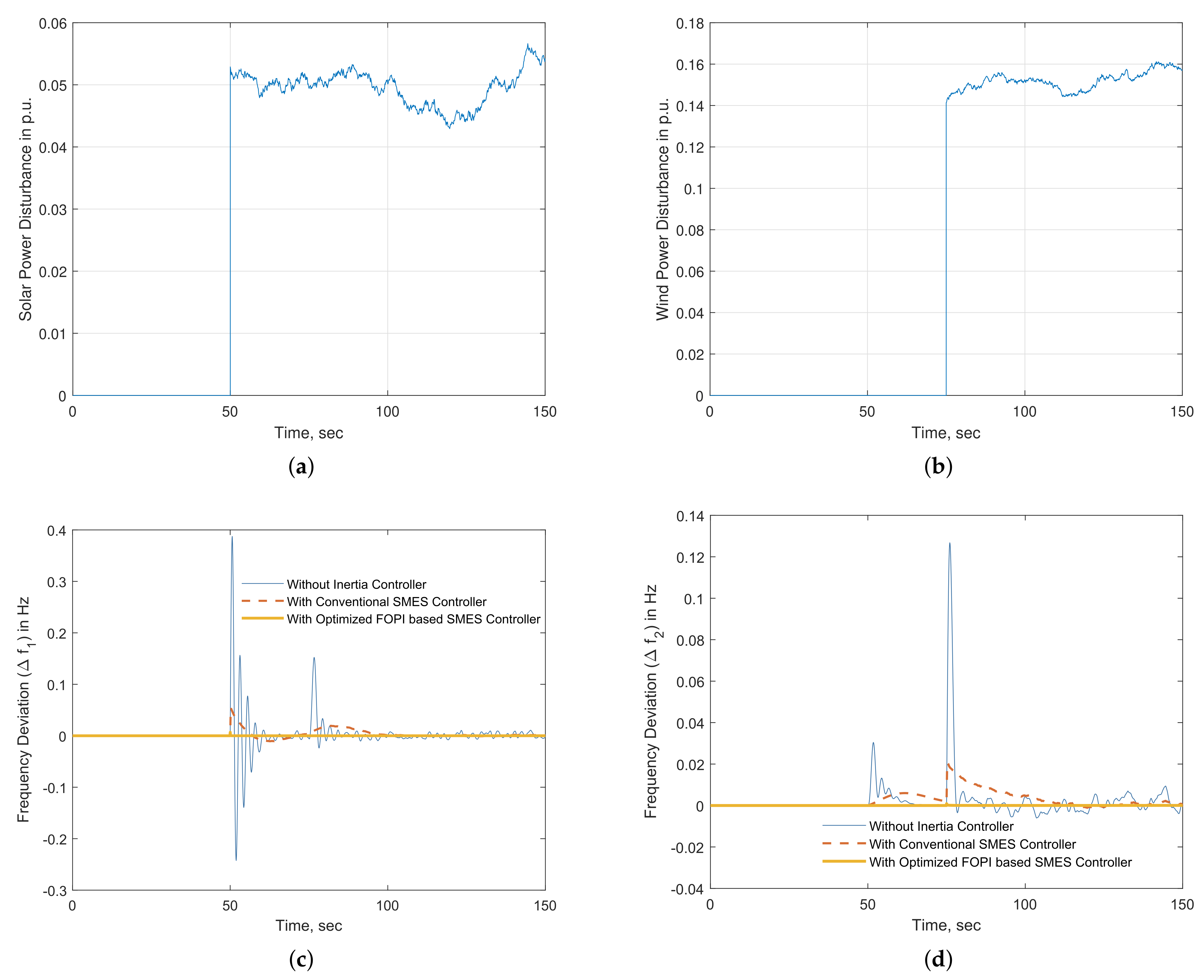
4.3. Controller Performance with Solar PV and Wind Power Fluctuations
The effectiveness of the proposed controller was also tested with fluctuating solar and wind power in both areas. The intermittent solar and wind power disturbances considered in this study are depicted in Figure 10a,b, respectively. The solar and wind powers have mean values of 0.05 p.u. and 0.15 p.u., respectively. The solar power is integrated in area 1 at 50 s during the 150 s simulation time, which continues to inject fluctuating power during the entire simulation period. On the other hand, the intermittent wind generating unit is connected at 75 s, which is kept connected throughout the entire simulation period. As shown in Figure 10c,d, the connection of varying solar and wind powers has a detrimental effect on system frequency response without any auxiliary controller.
The frequency of the system continues to vary during the entire simulation period and does not settle to a steady-state value. The conventional SMES controller slightly improves the system frequency response. On the other hand, the proposed controller performance is superior, in terms of settling time, overshoot, and undershoot, to the conventional SMES controller. The improvement of several performance indices is listed in Table 4 to demonstrate the superiority of the proposed controller.
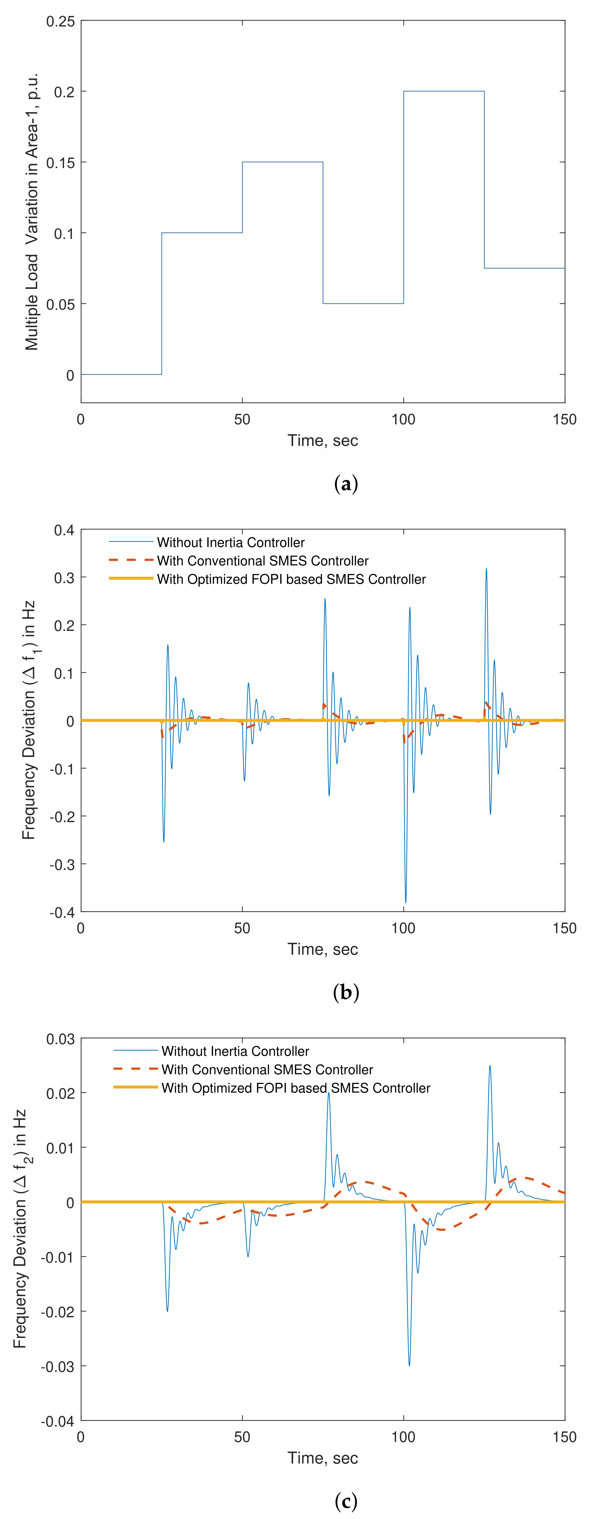
4.4. Frequency Response Analysis for Multiple Load Changes
The effectiveness and robustness of the proposed control technique for virtual control of low inertia systems were also tested with multiple load change scenarios. Several step load changes were considered, as shown in Figure 11a, to investigate the system capability to bring back the frequency deviation to zero before the next changes. Better performance of the proposed FOPI-based SMES is visible from the system frequency response, as seen in Figure 11b, following the first step load change of 0.1 p.u. at 25 s. The proposed controller is faster at eliminating the frequency deviation before the beginning of the second step load change of 0.15 p.u. at 50 s compared to conventional techniques. The frequency deviations in area 1 are very high at all points of step changes without a virtual inertia controller. Although the conventional SMES controller improves the frequency response slightly, a notable improvement is achieved with the proposed technique. In this case, also, the proposed method provides a much better performance in terms of overshoot, undershoot, and settling time. The frequency response for area 2 as visualized in Figure 11c shows better performance with the proposed control technique.
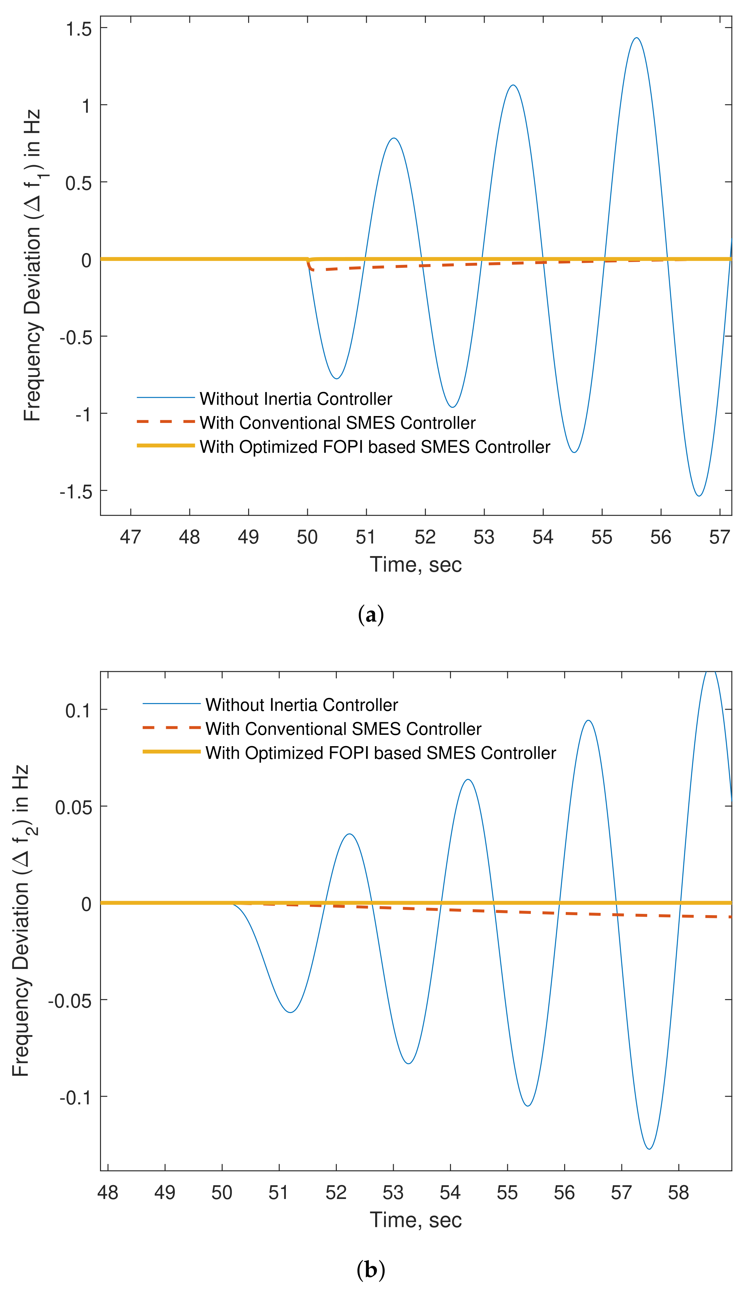
4.5. The Robust Performance of the Proposed Controller with the Reduced System Inertia
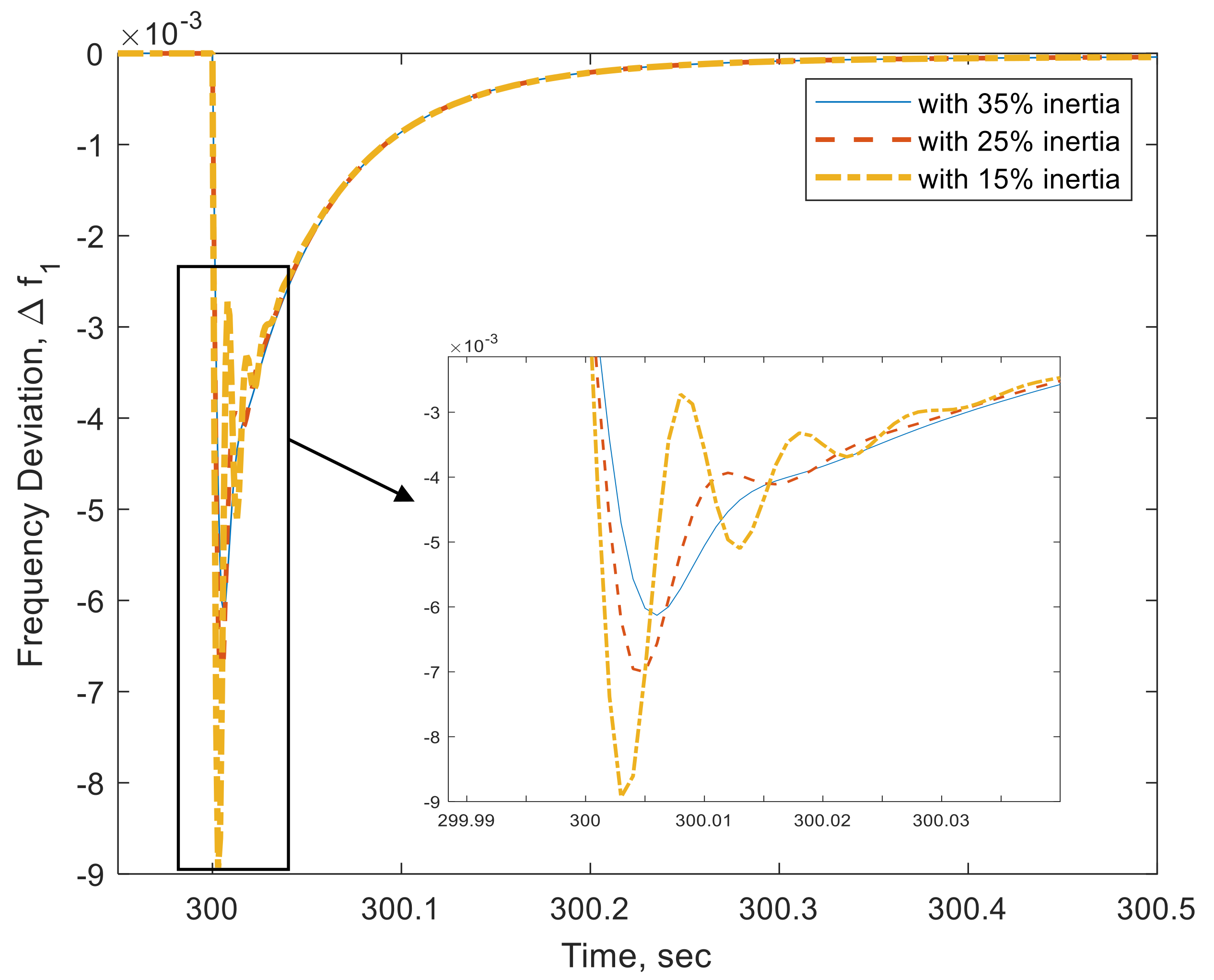
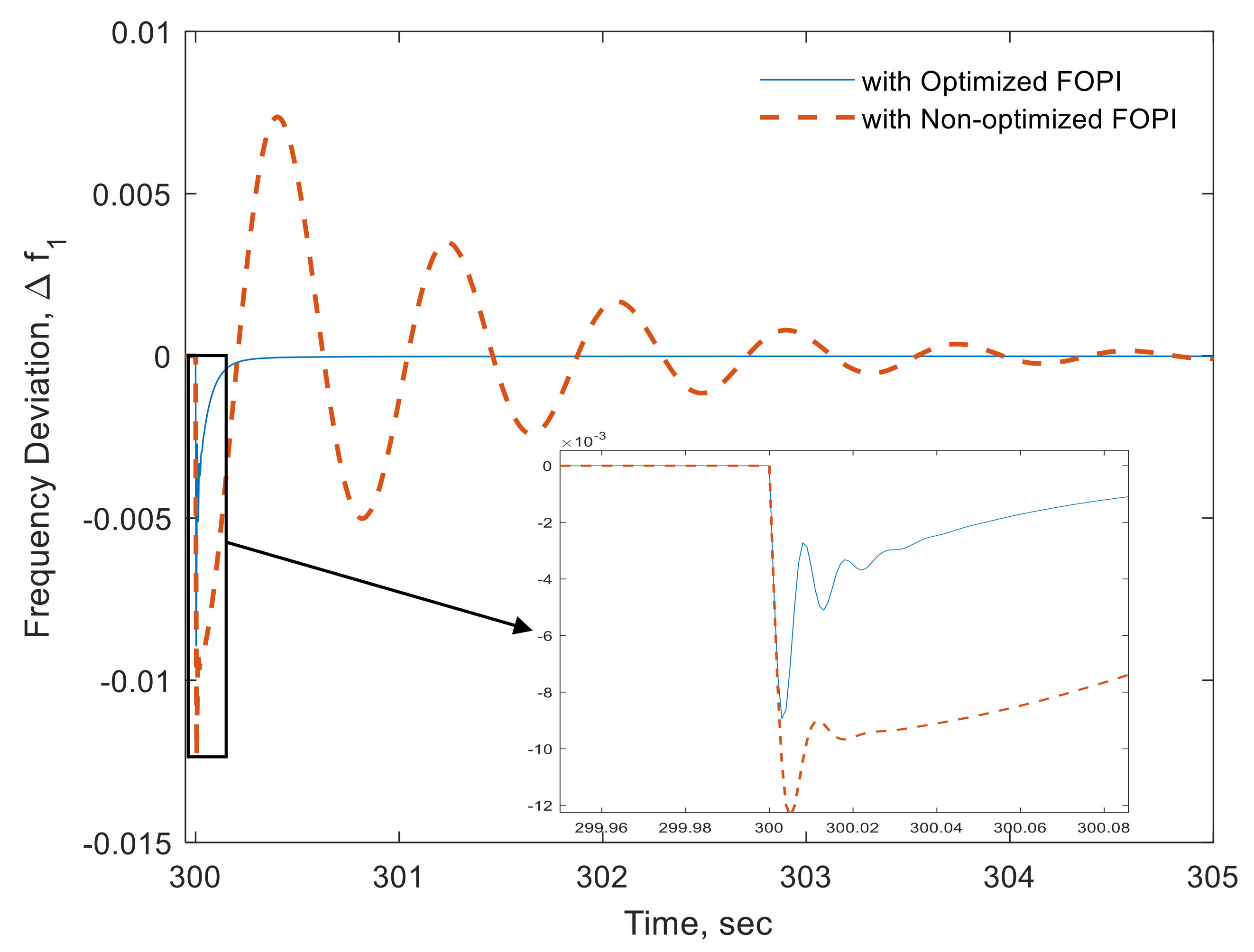
In this scenario, the robustness of the proposed controller is verified with the system inertia variations. The inertia in both areas is reduced by 50%, and a step load change of 0.15 p.u. is applied in area −1 at 50 s. The frequency response for this load change is depicted in Figure 12a,b. As depicted in Section 4.1, the system is capable of maintaining stable operation with a step load change of 0.15 p.u. in the case of default inertia (100%). However, Figure 12a,b show that the frequency deviations in both areas gradually increase, leading to instability. The system without SMES requires the under-frequency relay to start operation within 1 second of the load variation since the frequency deviation goes below 0.5 Hz, as depicted in Figure 12a. Although the area 2 frequency takes a longer time to operate under frequency relay, it is also unstable, as depicted by the increasing frequency oscillation in Figure 12b. The conventional SMES controller reduces the frequency deviations and stabilizes the system. However, the proposed control method augments the system stability greatly by reducing frequency deviations to almost zero even with 50% system inertia. The model presented in Figure 2 was also tested for very low inertia with a step load change of 0.1 p.u. in area 1. As shown in Figure 13, the controller is capable of stabilizing the model of Figure 2 for these low inertia. Furthermore, the robustness of the proposed optimized FOPI controller is compared with the non-optimized FOPI controller. The frequency deviation for the system with 15% inertia is plotted in Figure 14 with the optimized FOPI and non-optimized FOPI controller. Thus, the proposed controller is more robust compared to the conventional technique. The main limitation of the proposed technique is that the SMES is a costly solution. Further studies may be conducted on FOPI-based hybrid energy storage devices such as SMES, battery, and supercapacitor for the frequency control of low inertia PV/wind-integrated systems.
5. Conclusions
In this work, an optimized FOPI-based SMES virtual inertia controller is designed for a highly renewable energy integrated system. The dynamic model of the system is developed with FOPI to facilitate analysis and design of optimal parameters using PSO. The system response was analyzed with the designed virtual inertia controller considering highly fluctuating solar PV and wind energy. The system and the associated controllers were simulated in MATLAB Simulink. Small, medium, and large load disturbances were applied in the system to prove the effectiveness of the proposed energy storage-based virtual inertia control strategy. The system with default inertia and reduced inertia were tested under single and multiple load disturbances to guarantee the robustness of the proposed controller. The simulated results show promising performance in reducing system frequency deviations and in improving the frequency stability of the system. The proposed controller is superior to the conventional controller in reducing settling time, overshoot, and undershoot, as evident from the analysis. Moreover, the simulation outcomes prove the potential benefits of FOPI controller-based energy storage in high-level renewable energy integration and endorse the green efforts to improve sustainability. Finally, a detailed large-scale DFIG offshore wind farm model with FOPI-based hybrid energy storage virtual inertia controller can be studied as future work.
Author Contributions
Conceptualization, M.S.A.; methodology, M.S.A.; formal analysis, M.S.A., F.S.A.-I. and M.A.A.; writing—original draft preparation, M.S.A.; writing—review and editing, M.S.A. and F.S.A.-I.; supervision, M.A.A.; and funding acquisition, M.S.A. and F.S.A.-I. All authors have read and agreed to the published version of the manuscript.
Funding
This research received no external funding.
Institutional Review Board Statement
Not applicable.
Informed Consent Statement
Not applicable.
Data Availability Statement
Not applicable.
Acknowledgments
The authors acknowledge the support provided by King Fahd University of Petroleum & Minerals (KFUPM) through the directly funded project No. DF201022. The authors also acknowledge the funding support provided by K.A.CARE Energy Research & Innovation Center (ERIC), KFUPM, Dhahran, Saudi Arabia.
Conflicts of Interest
The authors declare no conflict of interest.
Abbreviations
The following abbreviations are used in this manuscript:
| RESs | Renewable energy sources |
| RoCoF | Rate of change of frequency |
| FOPI | Fractional-order proportional integral |
| SMES | Superconducting magnetic energy storage |
| PV | Photovoltaic |
| RE | Renewable Energy |
| PI | Proportional integral |
| PID | Proportional integral derivative |
| DFIG | Doubly fed induction generator |
| CCFC | Capacity constrained frequency control |
| LFC | Load frequency control |
| AEC | Area control error |
| PSO | Particle swarm optimization |
| GDB | Governor dead band |
| ANFIS | Adaptive neuro fuzzy system |
| TCPS | Thyristor controlled phase shifter |
| ABC | Ant bee colony |
| SOA | Seeker optimization algorithm |
| HS | Harmony search |
| WF | Wind farm |
| GRC | Generation rate constraint |
| PCS | Power conversion system |
| SA | Solar array |
| ISE | Integral squared error |
References
- Yongning, C.; Yan, L.; Zhen, W.; Zhen, L.; Hongzhi, L.; Zhankui, Z. The Characteristics and Challenge on Large-Scale Renewable Energy Grid Integration. In Proceedings of the 2019 IEEE Innovative Smart Grid Technologies-Asia (ISGT Asia), Chengdu, China, 21–24 May 2019; pp. 1393–1398. [Google Scholar]
- Kumar, K.P.; Saravanan, B. Recent techniques to model uncertainties in power generation from renewable energy sources and loads in microgrids—A review. Renew. Sustain. Energy Rev. 2017, 71, 348–358. [Google Scholar] [CrossRef]
- Samani, A.E.; D’Amicis, A.; De Kooning, J.D.; Bozalakov, D.; Silva, P.; Vandevelde, L. Grid balancing with a large-scale electrolyser providing primary reserve. IET Renew. Power Gener. 2020, 14, 3070–3078. [Google Scholar] [CrossRef]
- Dadkhah, A.; Bozalakov, D.; De Kooning, J.D.; Vandevelde, L. On the optimal planning of a hydrogen refuelling station participating in the electricity and balancing markets. Int. J. Hydrog. Energy 2021, 46, 1488–1500. [Google Scholar] [CrossRef]
- Alam, M.S.; Al-Ismail, F.S.; Salem, A.; Abido, M.A. High-Level Penetration of Renewable Energy Sources Into Grid Utility: Challenges and Solutions. IEEE Access 2020, 8, 190277–190299. [Google Scholar] [CrossRef]
- Morren, J.; De Haan, S.W.; Kling, W.L.; Ferreira, J. Wind turbines emulating inertia and supporting primary frequency control. IEEE Trans. Power Syst. 2006, 21, 433–434. [Google Scholar] [CrossRef]
- Fini, M.H.; Golshan, M.E.H. Frequency control using loads and generators capacity in power systems with a high penetration of renewables. Electr. Power Syst. Res. 2019, 166, 43–51. [Google Scholar] [CrossRef]
- Ulbig, A.; Borsche, T.S.; Andersson, G. Impact of low rotational inertia on power system stability and operation. IFAC Proc. Vol. 2014, 47, 7290–7297. [Google Scholar] [CrossRef] [Green Version]
- Saxena, P.; Singh, N.; Pandey, A.K. Enhancing the dynamic performance of microgrid using derivative controlled solar and energy storage based virtual inertia system. J. Energy Storage 2020, 31, 101613. [Google Scholar] [CrossRef]
- Pradhan, C.; Bhende, C. Enhancement in primary frequency contribution using dynamic deloading of wind turbines. IFAC-PapersOnLine 2015, 48, 13–18. [Google Scholar] [CrossRef]
- Ma, H.; Chowdhury, B. Working towards frequency regulation with wind plants: Combined control approaches. IET Renew. Power Gener. 2010, 4, 308–316. [Google Scholar] [CrossRef]
- Khooban, M.H.; Niknam, T. A new intelligent online fuzzy tuning approach for multi-area load frequency control: Self Adaptive Modified Bat Algorithm. Int. J. Electr. Power Energy Syst. 2015, 71, 254–261. [Google Scholar] [CrossRef]
- Magdy, G.; Mohamed, E.A.; Shabib, G.; Elbaset, A.A.; Mitani, Y. SMES based a new PID controller for frequency stability of a real hybrid power system considering high wind power penetration. IET Renew. Power Gener. 2018, 12, 1304–1313. [Google Scholar] [CrossRef]
- Cominos, P.; Munro, N. PID controllers: Recent tuning methods and design to specification. IEE Proc. Control Theory Appl. 2002, 149, 46–53. [Google Scholar] [CrossRef]
- Yang, L.; Hu, Z.; Xie, S.; Kong, S.; Lin, W. Adjustable virtual inertia control of supercapacitors in PV-based AC microgrid cluster. Electr. Power Syst. Res. 2019, 173, 71–85. [Google Scholar] [CrossRef]
- Magdy, G.; Shabib, G.; Elbaset, A.A.; Mitani, Y. A novel coordination scheme of virtual inertia control and digital protection for microgrid dynamic security considering high renewable energy penetration. IET Renew. Power Gener. 2018, 13, 462–474. [Google Scholar] [CrossRef]
- Kerdphol, T.; Watanabe, M.; Mitani, Y.; Phunpeng, V. Applying Virtual Inertia Control Topology to SMES System for Frequency Stability Improvement of Low-Inertia Microgrids Driven by High Renewables. Energies 2019, 12, 3902. [Google Scholar] [CrossRef] [Green Version]
- Gomez, L.; Grilo, A.P.; Salles, M.; Sguarezi Filho, A. Combined Control of DFIG-Based Wind Turbine and Battery Energy Storage System for Frequency Response in Microgrids. Energies 2020, 13, 894. [Google Scholar] [CrossRef] [Green Version]
- Kerdphol, T.; Watanabe, M.; Hongesombut, K.; Mitani, Y. Self-Adaptive Virtual Inertia Control-Based Fuzzy Logic to Improve Frequency Stability of Microgrid With High Renewable Penetration. IEEE Access 2019, 7, 76071–76083. [Google Scholar] [CrossRef]
- Kim, J.; Muljadi, E.; Gevorgian, V.; Mohanpurkar, M.; Luo, Y.; Hovsapian, R.; Koritarov, V. Capability-coordinated frequency control scheme of a virtual power plant with renewable energy sources. IET Gener. Transm. Distrib. 2019, 13, 3642–3648. [Google Scholar] [CrossRef]
- Abo-Elyousr, F.K.; Abdelaziz, A.Y. A Novel Modified Robust Load Frequency Control for Mass-Less Inertia Photovoltaics Penetrations via Hybrid PSO-WOA Approach. Electr. Power Compon. Syst. 2019, 47, 1744–1758. [Google Scholar] [CrossRef]
- Yap, K.Y.; Sarimuthu, C.R.; Lim, J.M.Y. Grid Integration of Solar Photovoltaic System Using Machine Learning-Based Virtual Inertia Synthetization in Synchronverter. IEEE Access 2020, 8, 49961–49976. [Google Scholar] [CrossRef]
- Rahman, F.S.; Kerdphol, T.; Watanabe, M.; Mitani, Y. Optimization of virtual inertia considering system frequency protection scheme. Electr. Power Syst. Res. 2019, 170, 294–302. [Google Scholar] [CrossRef]
- Zhang, X.; Zhu, Z.; Fu, Y.; Li, L. Optimized virtual inertia of wind turbine for rotor angle stability in interconnected power systems. Electr. Power Syst. Res. 2020, 180, 106157. [Google Scholar] [CrossRef]
- Pappachen, A.; Fathima, A.P. Load frequency control in deregulated power system integrated with SMES–TCPS combination using ANFIS controller. Int. J. Electr. Power Energy Syst. 2016, 82, 519–534. [Google Scholar] [CrossRef]
- Ali, M.H.; Wu, B.; Dougal, R.A. An overview of SMES applications in power and energy systems. IEEE Trans. Sustain. Energy 2010, 1, 38–47. [Google Scholar] [CrossRef]
- Shayeghi, H.; Jalili, A.; Shayanfar, H. A robust mixed H2/Hinf based LFC of a deregulated power system including SMES. Energy Convers. Manag. 2008, 49, 2656–2668. [Google Scholar] [CrossRef]
- Ngamroo, I.; Karaipoom, T. Cooperative control of SFCL and SMES for enhancing fault ride through capability and smoothing power fluctuation of DFIG wind farm. IEEE Trans. Appl. Supercond. 2014, 24, 1–4. [Google Scholar] [CrossRef]
- Ali, M.H.; Park, M.; Yu, I.K.; Murata, T.; Tamura, J.; Wu, B. Enhancement of transient stability by fuzzy logic-controlled SMES considering communication delay. Int. J. Electr. Power Energy Syst. 2009, 31, 402–408. [Google Scholar] [CrossRef]
- Chen, L.; Chen, H.; Yang, J.; Yu, Y.; Zhen, K.; Liu, Y.; Ren, L. Coordinated control of superconducting fault current limiter and superconducting magnetic energy storage for transient performance enhancement of grid-connected photovoltaic generation system. Energies 2017, 10, 56. [Google Scholar] [CrossRef] [Green Version]
- Abu-Siada, A.; Islam, S. Application of SMES unit in improving the performance of an AC/DC power system. IEEE Trans. Sustain. Energy 2010, 2, 109–121. [Google Scholar] [CrossRef]
- Podlubny, I. Fractional-order systems and PIλDμ controllers. IEEE Trans. Autom. Control 1999, 44, 208–214. [Google Scholar] [CrossRef]
- Li, H.; Luo, Y.; Chen, Y. A fractional order proportional and derivative (FOPD) motion controller: Tuning rule and experiments. IEEE Trans. Control Syst. Technol. 2009, 18, 516–520. [Google Scholar] [CrossRef]
- Komathi, C.; Umamaheswari, M. Design of Gray Wolf Optimizer Algorithm-Based Fractional Order PI Controller for Power Factor Correction in SMPS Applications. IEEE Trans. Power Electron. 2019, 35, 2100–2118. [Google Scholar] [CrossRef]
- Kesarkar, A.A.; Selvaganesan, N. Tuning of optimal fractional-order PID controller using an artificial bee colony algorithm. Syst. Sci. Control Eng. 2015, 3, 99–105. [Google Scholar] [CrossRef] [Green Version]
- Kumar, M.R.; Deepak, V.; Ghosh, S. Fractional-order controller design in frequency domain using an improved nonlinear adaptive seeker optimization algorithm. Turk. J. Electr. Eng. Comput. Sci. 2017, 25, 4299–4310. [Google Scholar] [CrossRef]
- Mosaad, M.I. Direct power control of SRG-based WECSs using optimised fractional-order PI controller. IET Electr. Power Appl. 2020, 14, 409–417. [Google Scholar] [CrossRef]
- Alam, M.; Alotaibi, M.A.; Alam, M.A.; Hossain, M.; Shafiullah, M.; Al-Ismail, F.S.; Rashid, M.; Ur, M.; Abido, M.A. High-Level Renewable Energy Integrated System Frequency Control with SMES-Based Optimized Fractional Order Controller. Electronics 2021, 10, 511. [Google Scholar] [CrossRef]
- Lee, D.J.; Wang, L. Small-signal stability analysis of an autonomous hybrid renewable energy power generation/energy storage system part I: Time-domain simulations. IEEE Trans. Energy Convers. 2008, 23, 311–320. [Google Scholar] [CrossRef]
- Bevrani, H.; Habibi, F.; Babahajyani, P.; Watanabe, M.; Mitani, Y. Intelligent frequency control in an AC microgrid: Online PSO-based fuzzy tuning approach. IEEE Trans. Smart Grid 2012, 3, 1935–1944. [Google Scholar] [CrossRef]
- Bevrani, H. Robust Power System Frequency Control; Springer: Boston, MA, USA, 2009; Volume 85. [Google Scholar]
- Tripathy, S.; Balasubramanian, R.; Nair, P. Effect of superconducting magnetic energy storage on automatic generation control considering governor deadband and boiler dynamics. IEEE Trans. Power Syst. 1992, 7, 1266–1273. [Google Scholar] [CrossRef]
- Eberhart, R.; Kennedy, J. A new optimizer using particle swarm theory. In Proceedings of the MHS’95, Sixth International Symposium on Micro Machine and Human Science, Nagoya, Japan, 4–6 October 1995; pp. 39–43. [Google Scholar]
- Tasgetiren, M.F.; Sevkli, M.; Liang, Y.C.; Gencyilmaz, G. Particle swarm optimization algorithm for permutation flowshop sequencing problem. In Proceedings of the International Workshop on Ant Colony Optimization and Swarm Intelligence, Brussels, Belgium, 5–8 September 2004; pp. 382–389. [Google Scholar]
- Engelbretch, A. Fundamentals of Computational Swarm Intelligence; John Wiley & Sons Ltd.: Oxford, UK, 2005; pp. 5–129. [Google Scholar]
- Abdel-Magid, Y.L.; Abido, M.A. AGC tuning of interconnected reheat thermal systems with particle swarm optimization. In Proceedings of the 10th IEEE International Conference on Electronics, Circuits and Systems, Sharjah, United Arab Emirates, 14–17 December 2003; Volume 1, pp. 376–379. [Google Scholar]
- Hossain, M.A.; Pota, H.R.; Squartini, S.; Zaman, F.; Guerrero, J.M. Energy scheduling of community microgrid with battery cost using particle swarm optimisation. Appl. Energy 2019, 254, 113723. [Google Scholar] [CrossRef]
- Aguilar, M.E.B.; Coury, D.V.; Reginatto, R.; Monaro, R.M. Multi-objective PSO applied to PI control of DFIG wind turbine under electrical fault conditions. Electr. Power Syst. Res. 2020, 180, 106081. [Google Scholar] [CrossRef]
- Kanwar, N.; Gupta, N.; Niazi, K.; Swarnkar, A.; Bansal, R. Simultaneous allocation of distributed energy resource using improved particle swarm optimization. Appl. Energy 2017, 185, 1684–1693. [Google Scholar] [CrossRef]
- Obaid, Z.A.; Cipcigan, L.M.; Abrahim, L.; Muhssin, M.T. Frequency control of future power systems: Reviewing and evaluating challenges and new control methods. J. Mod. Power Syst. Clean Energy 2019, 7, 9–25. [Google Scholar] [CrossRef]
Figure 1.
Two-area low inertia interconnected power system.

Figure 2.
The dynamic model of low inertia system with the proposed controller.

Figure 3.
SMES basic configuration.

Figure 4.
The dynamic SMES model along with the FOPI controller.

Figure 5.
PI controller (fractional order and integer order).

Figure 6.
The PSO flowchart for optimizing control parameters.

Figure 7.
The convergence of the cost function.

Figure 8.
Performance improvement with the proposed controller for load disturbances in area 1. (a) Area 1 frequency response for a 0.1 p.u. step load change. (b) Area 2 frequency response for a 0.1 p.u. step load change. (c) Area 1 frequency response for a 0.2 p.u. step load change. (d) Area 2 frequency response for a 0.2 p.u. step load change. (e) Area 1 frequency response for a 0.35 p.u. step load change. (f) Area 2 frequency response for a 0.35 p.u. step load change.

Figure 9.
Performance improvement with the proposed controller for load disturbances in area 2. (a) Area 1 frequency response for a 0.1 p.u. step load change. (b) Area 2 frequency response for a 0.1 p.u. step load change. (c) Area 1 frequency response for a 0.2 p.u. step load change. (d) Area 2 frequency response for a 0.2 p.u. step load change. (e) Area 1 frequency response for a 0.35 p.u. step load change. (f) Area 2 frequency response for a 0.35 p.u. step load change.

Figure 10.
The frequency response for wind generation addition at 50 s and solar generation addition at 75 s. (a) Solar power disturbance. (b) Wind power disturbance. (c) Area 1 frequency response for intermittent solar and wind power. (d) Area 2 frequency response for intermittent solar and wind power.

Figure 11.
(a) Multiple load variations in area 1. (b) Frequency response in area 1. (c) Frequency response in area 2.
Figure 11.
(a) Multiple load variations in area 1. (b) Frequency response in area 1. (c) Frequency response in area 2.

Figure 12.
System response for 50% inertia (a) Area 1 frequency response. (b) Area -2 frequency response.
Figure 12.
System response for 50% inertia (a) Area 1 frequency response. (b) Area -2 frequency response.

Figure 13.
The system response for very low inertia.

Figure 14.
The frequency response comparison for the optimized and non-optimized FOPI controllers.


Table 1.
System parameters for simulation.
| Parameters | Value | |
|---|---|---|
| Area-1 | Area-2 | |
| Inertia (p.u. MW s) | 0.079 | 0.11 |
| Damping constant (p.u. MW/Hz) | 0.016 | 0.017 |
| Time constant of solar system (s) | 1.2 | 1.2 |
| Time constant of wind system (s) | 1.4 | 1.4 |
| Frequency bias factor (p.u. MW/Hz) | 0.3585 | 0.3928 |
| Valve gate maximum limit (p.u. MW) | 0.5 | 0.5 |
| Valve gate minimum limit (p.u. MW) | −0.5 | −0.5 |
| Synchronizing coefficient (p.u. MW/Hz) | 0.09 | 0.09 |
| Area capacity ratio | −0.055 | −0.055 |
| Generation rate constraint (GRC) | 0.3 | 0.3 |
| Thermal generator (MW) | 12 | 15 |
| Wind generator (MW) | 8 | 8 |
| PV generator (MW) | 6 | 6 |
| Energy storage power rating (MW) | 3 | 3 |
| Energy storage inductor (H) | 2.65 | 2.65 |
| Energy storage time constant (s) | 0.05 | 0.05 |
| Energy storage reference current (kA) | 4.5 | 4.5 |
Table 2.
PSO-optimized FOPI and SMES parameters.
| Optimzed Parameters | |||
|---|---|---|---|
| Name | Value | Name | Value |
| 6.8650 | 0.1931 | ||
| 117.60 | 0.5000 | ||
| 0.9603 | 2.9782 | ||
| 21.660 | 0.1300 | ||
| 78.820 | 2.4879 | ||
| 0.6855 | 0.0410 | ||
Table 3.
Reduction in frequency deviations in area 1 and area 2 with the proposed controller.
| Frequency Deviation | |||||||
|---|---|---|---|---|---|---|---|
| (Hz) | (Hz) | ||||||
| Area | Step Load Change in p.u. | without Inertia Controller | Conventional SMES Controller | FOPI Based SMES | without Inertia Controller | Conventional SMES Controller | FOPI Based SMES |
| Area-1 | 0.1 | 0.420 | 0.035 | 0.005 | 0.020 | 0.004 | 4.0 |
| 0.2 | 0.850 | 0.080 | 0.010 | 0.040 | 0.008 | 3.2 | |
| 0.35 | unstable | 0.120 | 0.040 | unstable | 0.030 | 2.1 | |
| Area-2 | 0.1 | 0.395 | 0.025 | 1.9 | 0.320 | 0.030 | 0.010 |
| 0.2 | 0.840 | 0.060 | 1.2 | 0.630 | 0.090 | 0.012 | |
| 0.35 | 2.650 | 0.150 | 1.0 | 2.125 | 0.106 | 0.025 | |
Table 4.
Improvement of the performance indices for intermittent solar and wind power integration.
| Performance Indices | without Inertia Controller | Conventional SMES | Optimized FOPI Based SMES |
|---|---|---|---|
| Maximum Overshoot, Hz | 0.39 | 0.05 | 0.0100 |
| Maximum Undershoot, Hz | 0.25 | 0.01 | 0.0001 |
| Settling Time, Sec | inf | 50 | 2 |
Publisher’s Note: MDPI stays neutral with regard to jurisdictional claims in published maps and institutional affiliations. |
© 2021 by the authors. Licensee MDPI, Basel, Switzerland. This article is an open access article distributed under the terms and conditions of the Creative Commons Attribution (CC BY) license (https://creativecommons.org/licenses/by/4.0/).
Share and Cite
MDPI and ACS Style
Alam, M.S.; Al-Ismail, F.S.; Abido, M.A. PV/Wind-Integrated Low-Inertia System Frequency Control: PSO-Optimized Fractional-Order PI-Based SMES Approach. Sustainability 2021, 13, 7622. https://0-doi-org.brum.beds.ac.uk/10.3390/su13147622
AMA Style
Alam MS, Al-Ismail FS, Abido MA. PV/Wind-Integrated Low-Inertia System Frequency Control: PSO-Optimized Fractional-Order PI-Based SMES Approach. Sustainability. 2021; 13(14):7622. https://0-doi-org.brum.beds.ac.uk/10.3390/su13147622
Chicago/Turabian StyleAlam, Md Shafiul, Fahad Saleh Al-Ismail, and Mohammad Ali Abido. 2021. "PV/Wind-Integrated Low-Inertia System Frequency Control: PSO-Optimized Fractional-Order PI-Based SMES Approach" Sustainability 13, no. 14: 7622. https://0-doi-org.brum.beds.ac.uk/10.3390/su13147622
Note that from the first issue of 2016, this journal uses article numbers instead of page numbers. See further details here.