
A Combined Control Systems and Machine Learning Approach to Forecasting Iceberg Flux off Newfoundland


1
Department of Geography, University of Sheffield, Sheffield S10 2TN, UK
2
School of Aerospace, Transport and Manufacturing, Cranfield University, Cranfield MK43 0AL, UK
3
School of Geography and Lincoln Centre for Water and Planetary Health, University of Lincoln, Lincoln LN6 7FL, UK
*
Author to whom correspondence should be addressed.
Sustainability 2021, 13(14), 7705; https://0-doi-org.brum.beds.ac.uk/10.3390/su13147705
Submission received: 25 May 2021
/
Revised: 23 June 2021
/
Accepted: 7 July 2021
/
Published: 9 July 2021
(This article belongs to the Special Issue Modelling for Sustainable Marine Management)
Abstract
:Icebergs have long been a threat to shipping in the NW Atlantic and the iceberg season of February to late summer is monitored closely by the International Ice Patrol. However, reliable predictions of the severity of a season several months in advance would be useful for planning monitoring strategies and also for shipping companies in designing optimal routes across the North Atlantic for specific years. A seasonal forecast model of the build-up of seasonal iceberg numbers has recently become available, beginning to enable this longer-term planning of marine operations. Here we discuss extension of this control systems model to include more recent years within the trial ensemble sample set and also increasing the number of measures of the iceberg season that are considered within the forecast. These new measures include the seasonal iceberg total, the rate of change of the seasonal increase, the number of peaks in iceberg numbers experienced within a given season, and the timing of the peak(s). They are predicted by a range of machine learning tools. The skill levels of the new measures are tested, as is the impact of the extensions to the existing seasonal forecast model. We present a forecast for the 2021 iceberg season, predicting a medium iceberg year.
1. Introduction
Icebergs have been a threat to shipping in the North Atlantic since humans first ventured onto that stretch of ocean. They mostly originate from the Greenland Ice Sheet, which has increasingly been losing mass since the 1990s under climate warming [1]. The first recorded iceberg incident with North Atlantic shipping occurred in 1686, with the ‘Happy Return’ sinking in the Hudson Bay while on a trade operation for the North West Fur Company [2]. Hundreds of lives were lost in collisions in the following three centuries, with notable years include 1856, where over 300 people were killed in the first two months alone, and 1884, where 12 vessels were damaged or sunk [2]. While these sorts of tragedies were fairly common, the sinking of the RMS Titanic in 1912 with the loss of more than 1500 lives dramatically drew widespread public attention to iceberg risk. With 1038 icebergs recorded south of 48° N that year, this would have been a high ice year for the time, but not unusually so. There had been strong north to north-westerly winds that year, bringing very low temperatures, which facilitated icebergs surviving further south than the average, although not beyond the ice limit for the 20th century [3]. Therefore, while the iceberg risk for 1912 was high, it was not unprecedented, suggesting the need for a dedicated iceberg warning system.
The International Ice Patrol (IIP) was established in the following year to try and prevent any more such incidents occurring. Today, combining data compiled from air surveillance, ship reports, satellite analysis and iceberg trajectory models, the IIP release daily charts of iceberg locations and weekly outlooks that are distributed through the North American Ice Service (available at https://www.navcen.uscg.gov/?pageName=iipCharts&year=2021, accessed on 24 January 2021). In their hundred-year history, the IIP have significantly reduced the risk to life, with no human or major commercial losses in the patrolled region when vessels have followed IIP advice [4]. However, the potential for a major disaster still exists.
While short term forecasts reduce the risk of serious collisions, longer term predictions could have a significant impact on marine planning, potentially altering iceberg monitoring and even shipping routes months in advance. This would be of great economic benefit, particularly as in recent decades the mean annual iceberg numbers entering the shipping lanes of the NW Atlantic have significantly increased compared to earlier in the twentieth century [5], therefore raising the underlying risk to shipping.
Previous work on understanding the links between the NW Atlantic iceberg flux and potential environmental causes of variability in calving and in-ocean survival has shown a strong, although temporally evolving, non-linear connection between this iceberg number flux across 48° N, henceforth to be denoted I48N; lagged variation in the Greenland Ice Sheet surface mass balance (SMB, equivalent to snow accumulation minus surface meltwater runoff); the sea surface temperature (LSST) of the Labrador Sea through which the icebergs travel; and the dominant atmospheric variability of the region, the North Atlantic Oscillation Index (NAO) [5,6,7]. The imclusion of lagged non-linear relationships in these studies has raised the chance of seasonal forecasting being successful. Previous work looked at an adaptation of [7], where only lags of at least eight months are used in the Windowed Error Reduction Ratio (WERR) model linking I48N with the forcing terms of SMB, LSST, and NAO. This led to development of a seasonal forecast model for the next season’s I48N flux [8]. This was shown to have a skill level of 80% with respect to the high or low nature of I48N compared to the long-term mean. This seasonal iceberg forecast has now been issued each year to the International Ice Patrol since 2018.
Later discussions with the IIP suggested that the purely numerical forecast measure of the forthcoming iceberg season provided via the WERR model is not the only one of interest, and potential use, for seasonal iceberg risk evaluation [9]. This paper therefore develops new machine learning approaches to generating forecasts for other more holistic measures of the seasonal iceberg risk, and assesses their potential, as well as presenting improvements to the WERR control systems model.
2. Materials and Methods
2.1. Data
The three-monthly input variables for prediction of I48N for both the machine learning models and the WERR model are: SMB, which affects how many icebergs calve from Greenland; the NAO, which affects atmospheric temperatures and precipitation in the region; the mean Labrador Sea surface temperature (LSST), which affects both the calving rate of icebergs and the survivability of icebergs once in the ocean. The calculation method for Greenland SMB is given in [10,11], and is the difference between ice sheet mass gain from snow accumulation and mass loss from ice sheet meltwater runoff, based on positive degree day runoff retention modelling [12]. Here, SMB data extended to 2020, and based on newly-available European Centre for Medium-Range Weather Forecasts ERA-5 meteorological reanalysis data, are used. The LSST data can be found in the Physical Sciences Division of NOAA, under Kaplan v2 SST, and consists of monthly sea surface temperature anomalies in the Labrador Sea, over the area 67–55° N, 65–45° W (https://psl.noaa.gov/data/gridded/data.kaplan_sst.html, accessed on 24 January 2021). NAO data are available at https://www.cpc.ncep.noaa.gov/data/teledoc/nao.shtml, accessed on 24 January 2021.
I48N, the number of icebergs south of the 48th parallel in a given month as recorded by the IIP and available through their Annual Reports (see, for example [9]), is generally accepted to reflect annual variability in iceberg activity in the Labrador Sea [5]. The latitude of 48° N is also the point beyond which icebergs begin to enter the trans-Atlantic shipping lanes (Figure 1).
2.2. The WERR Control Systems Model
A model for I48N was developed in [5] using a Windowed Error Reduction Ratio (WERR) control systems method, where a sliding time-window, non-linear, and time-lagged polynomial regression model, forced with the three environmental factors of SMB, NAO, and LSST, is optimised for the observed number of icebergs passing 48° N. This method computes the linear and non-linear correlations between the input and output signals directly to select the model terms one by one. The full mathematical basis behind the WERR model can be seen in [7]. The WERR method was shown in [6] to produce an output that had a correlation of 0.84 with the annual variation in the number of icebergs passing 48° N between 1900 and 2008.
The original WERR model was a non-autocorrelative interpretative tool for I48N, rather than a predictive one, and therefore, polynomial terms with time lags between 0 and 48 months were allowed within the library of candidate terms available for the model optimisation [7]. However, the dominant terms in the original WERR model had a lag of eight months or longer, reflecting a minimum timescale between calving and icebergs reaching 48° N; therefore, the model was adapted for predictive purposes by only allowing polynomial terms with a lag of this size to be available during the model optimisation [8]. This predictive model has a reduced, however still statistically significant (at the 1% level), correlation of 0.60 between the January–September I48N values and the WERR model predictions over a 20 year test period, with a confidence of 80% in assessing whether a year was a high or low iceberg year relative to the 1997–2016 annual mean of 592.
Seasonal forecasts produced from an ensemble of sliding-temporal windows of this revised WERR model (see [8] for details) have been released to the IIP for several years. The ensemble nature of the forecasts gives a measure of the error through its standard deviation. In addition, to take account of the largely bimodal nature of the I48N iceberg number, [8] also categorized the forecasts as “high” or “low”, relative to the mean 1997–2016 I48N value of 497. Thus, the 2017 iceberg season forecast was 766 ± 297, with an observed total of 1008, this was therefore a formal success, and both forecast and observed numbers fall in the “high” category. In 2018 the forecast was 685 ± 207, with an observed number of 208. While the forecast was lower than the 2018 observed total, it was still “high”, while the observed I48N was clearly a “low” year, thus the 2018 forecast was a failure. The 2019 forecast was for 516 ± 150 icebergs. By the end of the season, the total number had reached 1515. The 2019 forecast was therefore a formal failure, although it was predicting a “high” year, as was observed. The 2020 forecast (including the machine learning approach) was for a low/medium ice year with 584 ± 303 icebergs by the end of July. The observed number by this point was 169 (personal communication, Michael Hicks, IIP), representing a “low” iceberg year. The observed 2020 iceberg number fell outside the error bars; however, there was an exceptionally large uncertainty in the 2020 forecast, with many of the ensemble numbers falling into the “low” category. This spread in the forecast probability amplified the need for alternative approaches; these are provided by the new machine learning models discussed below and it will be seen below that their forecast for 2020 was definitely for a “low” iceberg year.
As it was previously found that using WERR model ensemble members generated from more recent years seemed to produce closer ensemble results to reality than those earlier in the trial period, here, the 20-year WERR model training period has been moved forward two years to 2018 (see Table S1 and discussion in Section 3.1).
2.3. The New Iceberg Season Measures
While a prediction of the total number of icebergs past 48° N in an ice year is a useful tool in understanding iceberg risk, other factors, including how early and late in each season icebergs will enter the shipping lanes, are also of use to shipping. Therefore, three new measures have been included in the iceberg forecast, using a machine learning approach. These are a prediction of the peak month, the number of peaks, and the rate of change. The machine learning tools have also been used to create a forecast of the maximum annual I48N number to complement the WERR model prediction.
In an average year, North Atlantic icebergs are most prevalent in the months between March and June (Figure 2). However, which month contains the greatest flux, and so has the greatest risk to shipping, is variable. Therefore, a prediction for the month in which the ‘peak’ occurs has been made for the 2021 ice season, estimated based on monthly values. An outcome of ‘0’ reflects a prediction that the peak will occur between January and March. A result of ‘1’ reflects April, and ‘2’ denotes May. A value of ‘3’ suggests the peak month will be in June or later in the year.
Figure 2 also suggests that it is usual to have one dominant peak in monthly iceberg number, however, this is not necessarily the case. In some years, including 2019 [9], more than one peak was observed. Therefore, machine learning tools have been used to predict the number of peaks in the 2021 iceberg forecast. A result of ‘1’ suggests a single peak, whereas ‘2’ denotes a year with multiple peaks. As daily data are only available for the last decade, monthly values have been used to estimate whether a year had one or more peaks.
The rate of change prediction (RoC) is a measure of how rapidly icebergs are passing 48° N and entering the shipping lanes. Iceberg numbers can vary significantly in a short period of time, and having some warning of this would be of use to ship’s captains. Therefore, the maximum rate of increase in each ice year from 1900 to 2020 was calculated, and, when ordered, the lower third were categorised as low, ‘0’, the centre third as medium, or ‘1’, and the highest third as ‘2’, or high.
In addition to the measures predicting iceberg behaviour, a machine learning approach has also been used to predict the annual I48N total. Here, the categories are defined by the IIP; therefore, a low year, ‘0’, has less than 231 icebergs past 48° N, a medium year, ‘1’, has between 231 and 1036, and a high year, ‘2’, has more than 1036. In order to improve model accuracy, only three categories have been used for prediction; however, the IIP also includes a definition for an extremely high ice year of more than 1399 icebergs.
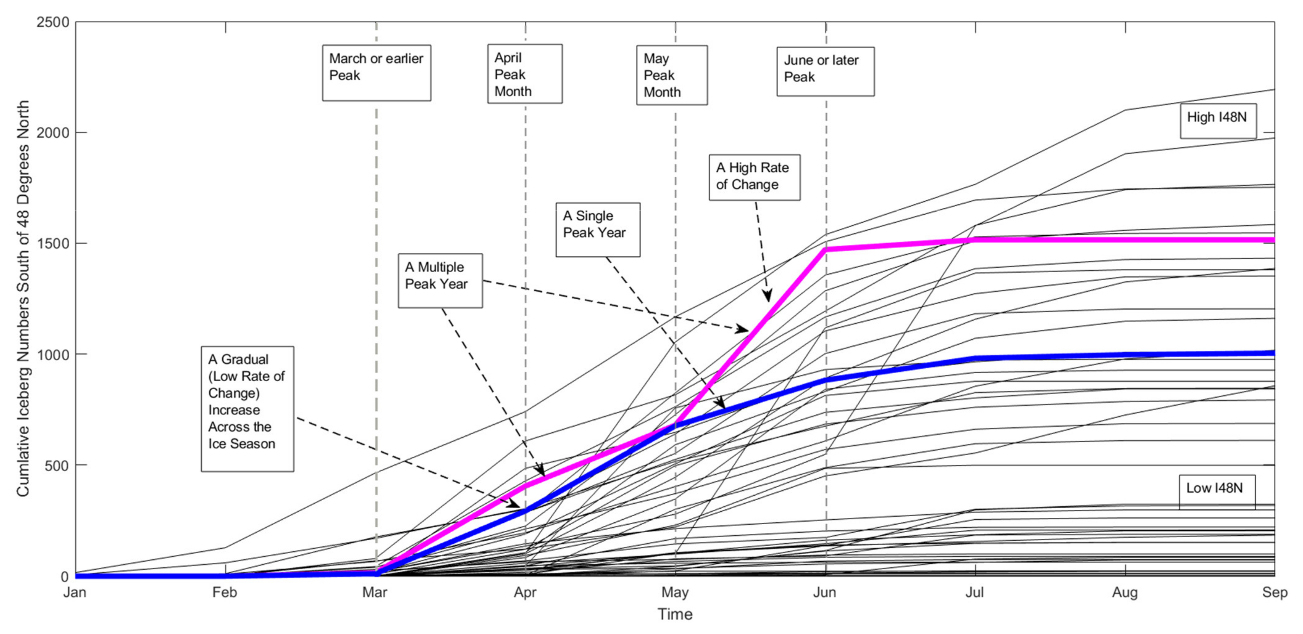
To graphically show the main features of an iceberg year for the new prediction measures, Figure 3 shows all these new measures. The new measures have been outlined on the plot and can be seen to represent the main differences between one iceberg year and another. Two recent years, 2017 and 2019, have been highlighted, as they show strong characteristics of particular measures. The magenta line, representing 2019, clearly shows a multiple peak year, with a high rate of change and a high I48N. As the most significant peak that year occurs in May, this is the peak month. The blue line, showing 2017, has a much gentler increase across the year, and therefore a low rate of change. As the greatest increase was in April, this is the peak month for that year. 2017 also only has one iceberg peak, and a medium I48N. The black lines show the last 50 years of cumulative iceberg numbers across the season. It can be seen that the greatest change in iceberg numbers usually occurs between March and June. Figure 3 also shows that there is high variation in the total I48N, ranging from 0 to more than 2000 icebergs in a year, with the low, medium, and high divisions being clear.
The three new measures allow for a better understanding of iceberg behaviour in past years. However, they are as complex to predict as I48N. This is often due to sea ice trapping icebergs along the coast and releasing them when temperatures increase, affecting the rate at which the icebergs pass 48° N and the month in which the peak occurs. This is also the dominant cause of a multiple peak year. LSST is used in the models to try and reflect this, as sea surface temperatures are strongly correlated to sea ice extent. Atmospheric temperatures, represented by the NAO, also contribute. Adding a sea ice input variable into the models was explored; however, it did not increase prediction accuracy.
2.4. The Machine Learning Models
For the new measures, three machine learning models were tested and compared: Linear Discriminant analysis, a Linear Support Vector Machine algorithm (SVM), and a Quadratic SVM algorithm. The models use knowledge of the annual means of the three environmental parameters forcing the control systems model (SMB, LSST and NAO), and allow a measure of auto-regression through having knowledge of the previous years’ value of the appropriate measure of the environmental parameters and I48N. While there are other machine learning models, such as Random Forest or Gradient Boosting, that could be considered, these particular models have been selected due to their strength in classification tasks [13]. It was found in [13] that the Linear Discriminant approach was best for model precision, especially in circumstances with relatively few input variables. It was also suggested that the SVM method has the potential to outperform all other surveyed models when the number of input variables increases. Therefore, these approaches seem to complement each other, and were also all shown to have predictive skill beyond random chance (see Section 3.2). It should be noted that this paper aims to demonstrate the proof-of-the-concept of machine learning for this specific application, rather than optimising their prediction performance. Further research could look at involving other relevant machine learning models for a comprehensive comparison of prediction performance.
The first approach, linear discriminant analysis, or the Fisher discriminant, has been a popular tool since 1936 [14]. While much has changed in the following years, the base application remains the same. Classification is achieved by imagining the data on a line, and maximising the distance between the different data class means [15]. Overall, it is a variable reduction technique with strong pattern recognition ability [16]. The wide range of real-world applications for this technique are a further testament to its longevity, appearing in fields from earthquake-induced liquefaction [17] to text classification [16].
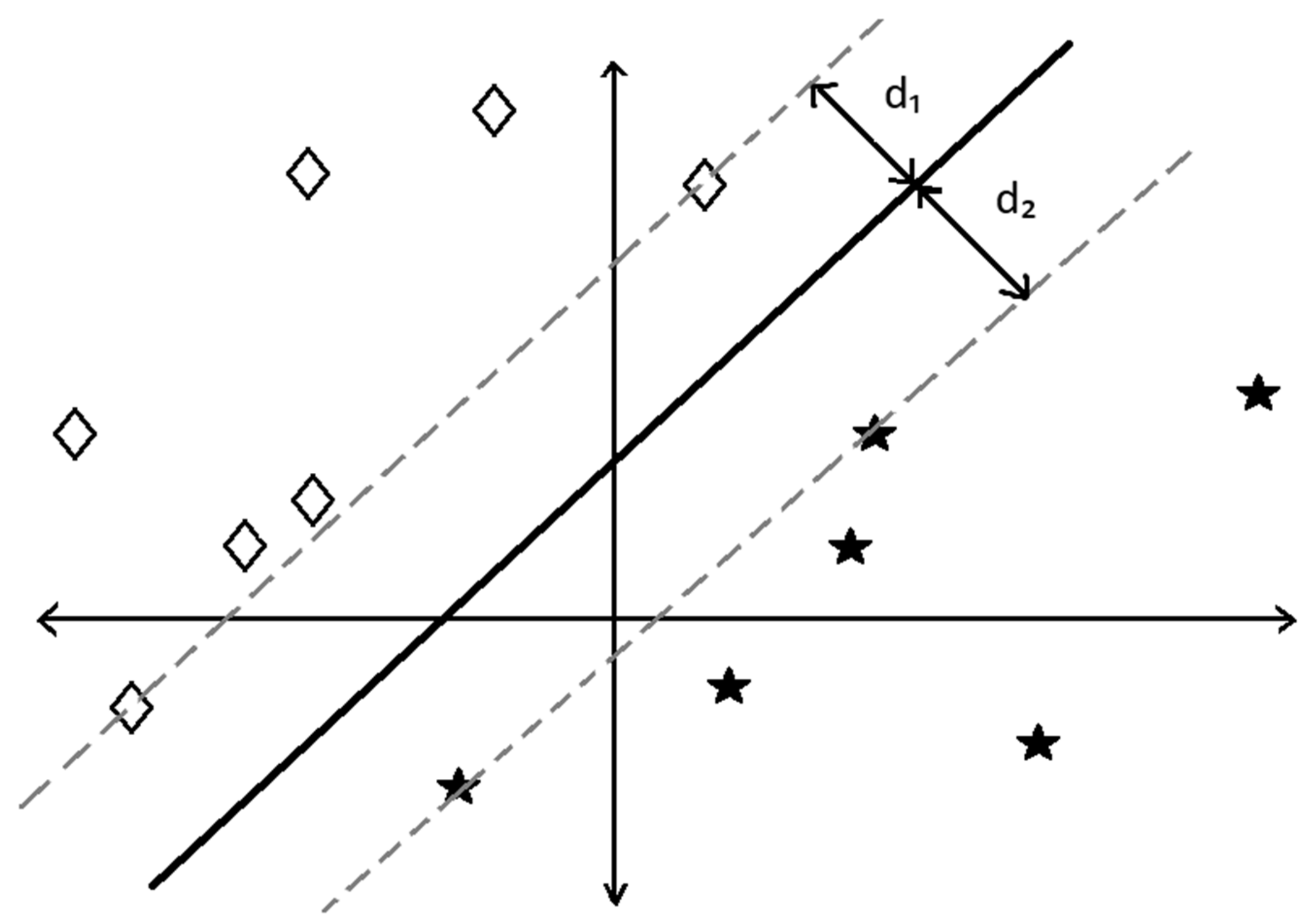
The other two approaches are linear and quadratic SVM algorithms. These are popular tools that attempt to locate an optimal boundary (or hyperplane) between classes for classification purposes [18]. A visualization of finding the optimal linear hyperplane can be seen in Figure 4. While a quadratic boundary between classes is less easy to envision, the general principle remains the same: divide the data into classes by finding the best possible boundary between them. Many examples of this practice can be seen in the medical field, in analyzing enzymes for liver disease [19] or diagnosing whether a tumour is malignant or benign [20]: however, examples are also beginning to be encountered in environmental sciences, such as flood classification [21] or crop disease assessment [22].
The machine learning models have been run through the MATLAB Classification Learner App. All three approaches were trained on a 30-year sliding-window method in order to utilise the relatively short dataset of yearly values since 1901, and for consistency with the WERR approach [6]. They are then tested on the following year, starting at 1931, rolling forward. An average accuracy and error value can then be calculated from the 86 runs per model, as opposed to having a single accuracy value (see results section for further discussion).
3. Results
3.1. Revised WERR Model Accuracy
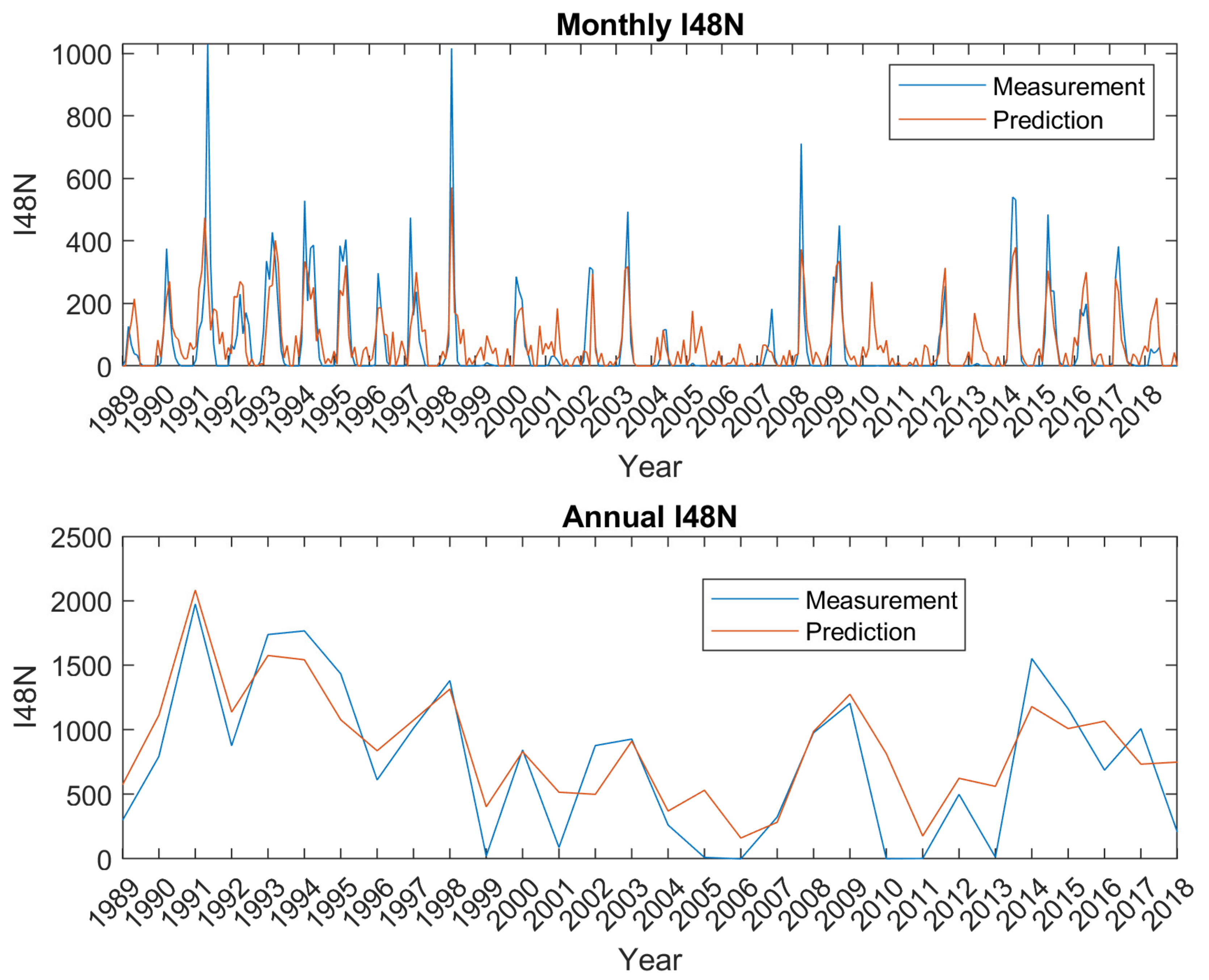
As previously stated, the WERR model training period was moved forward two years to 2018, compared to the model evaluated in [6,7]. Only the terms with a time lag time of at least eight months were selected, which allows production of a predictive model eight months ahead. The selected terms are also required to have an ERR (Error Reduction Ratio) of 0.02 or higher (see [7] for a definition of ERR). The time series of the performance of the WERR model over the latest 30-year period of 1989–2018 is shown in Figure 5. While the model often under-estimates the peak spring value of I48N, and over-estimates iceberg numbers in very low iceberg years, its representation of the annual cycle (upper panel) and the annual total (lower Panel) is good, with the latter having a statistically significant (at the 1% level) correlation of 0.87.
3.2. Sensitivity of the Machine Learning Tools
The average accuracy, F1 score, and root mean squared error (RMSE) of the various machine learning models can be seen in Table 1. When forecasting the I48N annual total, the output can either be low, medium, or high. As there are three possible outcomes, an accuracy of more than 33% is desirable to show that the method has some skill beyond random chance. Similarly, for the maximum rate of increase in an ice year forecast, there are also three outcomes: either low, medium or high. However, when forecasting the number of peaks in an ice year, there are only two possible outcomes: either one or multiple. Therefore, for the prediction to show skill beyond random chance, an accuracy of more than 50% is required. Lastly, for the prediction of when the peak month will occur in an ice year, there are four possible outcomes: January to March, April, May, or June onwards. This prediction therefore has the lowest requirement, of more than 25%, of performance better than random chance.
From Table 1, it can be seen that the three machine learning models have similar levels of accuracy and RMSE between models when considering each new measure. However, the skill level, defined as the mean model accuracy/(expected random accuracy), differs between measures modelled. The model of the annual I48N total is the most skillful by some margin, while the skill levels for models of each of the other three measures are similar. The F1 score, a measure of incorrectly classified cases, also agrees with this. While the number of peaks prediction has a higher F1 score than I48N, reflecting high model precision, this is offset by the forecast having the lowest number of possible outcomes. Similarly, the peak month prediction has the greatest number of outcomes, and therefore has an expected lower precision.
The Supplementary Materials (Figures S1–S4) provide a confusion matrix for each model for every measure for the 30-year sliding window used for the 2021 forecast. These reflect the complexity of forecasting these naturally highly variable measures, namely in the peak month and rate of change forecasts. However, the I48N matrices show how successful that aspect is in predicting iceberg severity. The confusion matrices for the number of peaks measure (Figure S3) reflect the greater number of one-year peaks than multiple-year peaks.
The forecast for a particular measure is defined as a collective view of the combined models of a given measure. While the models often agree on individual measures, the likelihood of the models predicting all four measures the same is low. For the 2021 forecast, when the models predicted different outcomes for a measure, the forecast was the outcome that had been predicted more than once. Section 3.4.3 discusses the merits of weighting the forecast, so that certain models’ outcomes are chosen over the others, even in the case of a majority, if that model was proven to be the best at representing the individual measure. However, at this stage, no definitive optimal model could be selected, resulting in taking the common prediction. Future work would aim to further clarify this matter.
3.3. Machine Learning Hindcasts
Previous WERR model forecasts were discussed in Section 2.2; here the 2017–2020 machine learning hindcasts are presented, and can be seen in Table 2. Interestingly, the Linear Discriminant and Linear SVM hindcasted the same result across all measures for the years 2017–2020; however, this was not the case for the 2021 forecast, discussed in Section 3.4.3, nor has this historically been the case.
The 2017 hindcast was for a medium iceberg year across all models, and this was the observed case. The three models also successfully hindcasted one peak. However, all models were incorrect in hindcasting a medium rate of change (observed low) and a peak month of May, as opposed to the true April. Overall, the hindcast was fairly successful, hindcasting both I48N and the number of peaks correctly. There was also high model unity between all measures.
For 2018, all models incorrectly hindcasted a medium iceberg year, when a low year was observed. While there is less agreement between the models for the other three measures, all incorrectly hindcasted the peak month (April and May, when January–March was observed). Only the Quadratic SVM successfully hindcasted the rate of change (medium); however, the Linear Discriminant and Linear SVM models successfully hindcasted the number of peaks (two) where the Quadratic SVM failed to do so. Overall, this hindcast was unsuccessful, with only individual models successfully hindcasting selected outcomes.
For the 2019 season, all models successfully hindcasted a high iceberg year; however, they also all failed to hindcast a second peak. Only the Quadratic SVM successfully hindcasted both the rate of change and the peak month (medium and May). Overall, the Quadratic SVM hindcast was very good for this year; however, the two linear models were less successful.
For the 2020 hindcast, both the Linear Discriminant and the Linear SVM successfully hindcasted a low iceberg year, and all models hindcasted one peak. However, no model hindcasted a high rate of change or that the peak would occur in April. Overall, the hindcast was fairly successful when looking at the linear models.
These hindcasts show that, while the individual models often fail to predict certain measures, it is common for at least one model to successfully predict an outcome. This is true for the long-term trend, not just the four years hindcasted here. Therefore, it is in deciding which model results should take precedence that further work on this topic would be of benefit.
3.4. The 2021 Forecast
3.4.1. The WERR Prediction
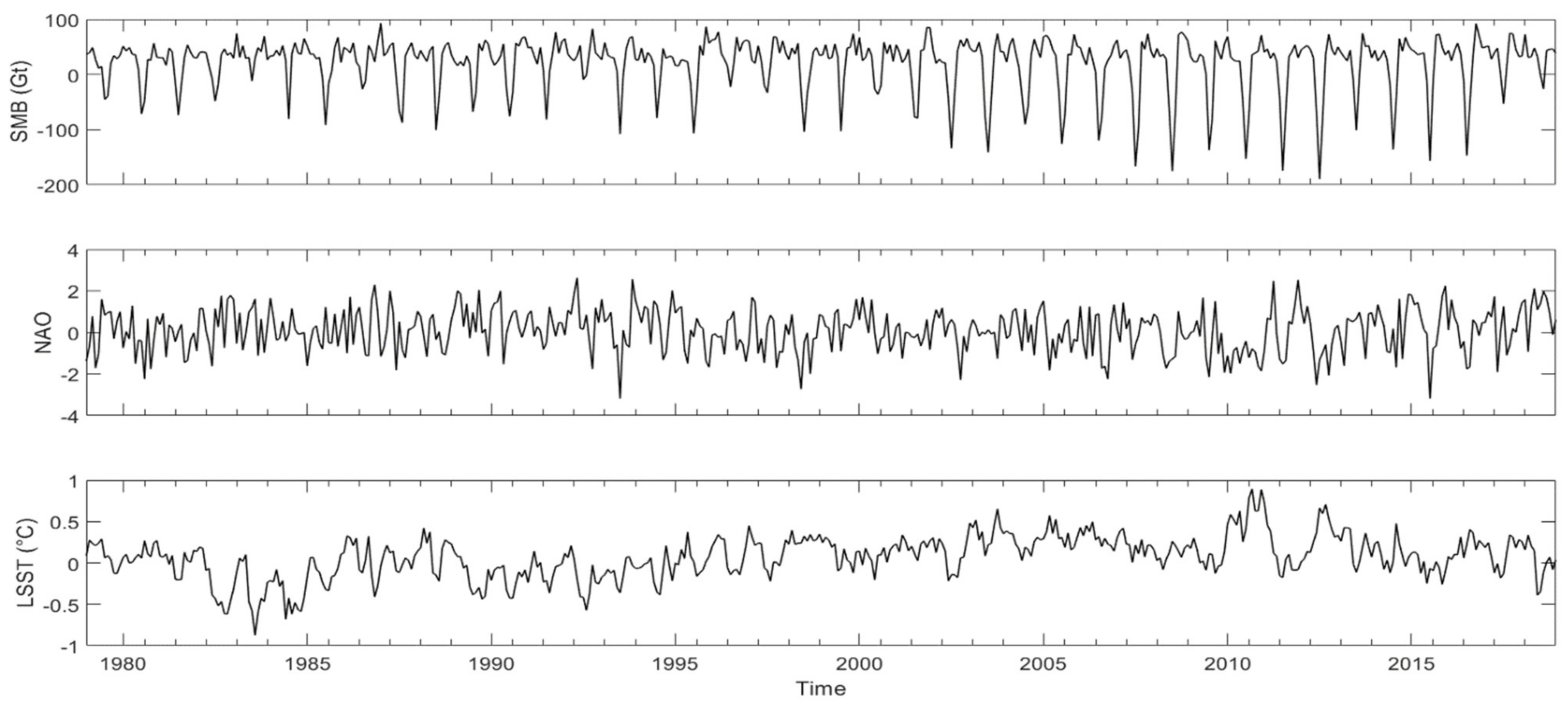
Following the approach of [7], using the forcing of the monthly series of SMB, LSST, and NAO shown in Figure 6 and an ensemble of WERR models for the 11 30-year sliding windows 1979–2008 through 1989–2018 shown in Table S1, the WERR 2021 forecast is 675 ± 123 icebergs. This is in keeping with a prediction of a medium ice year.
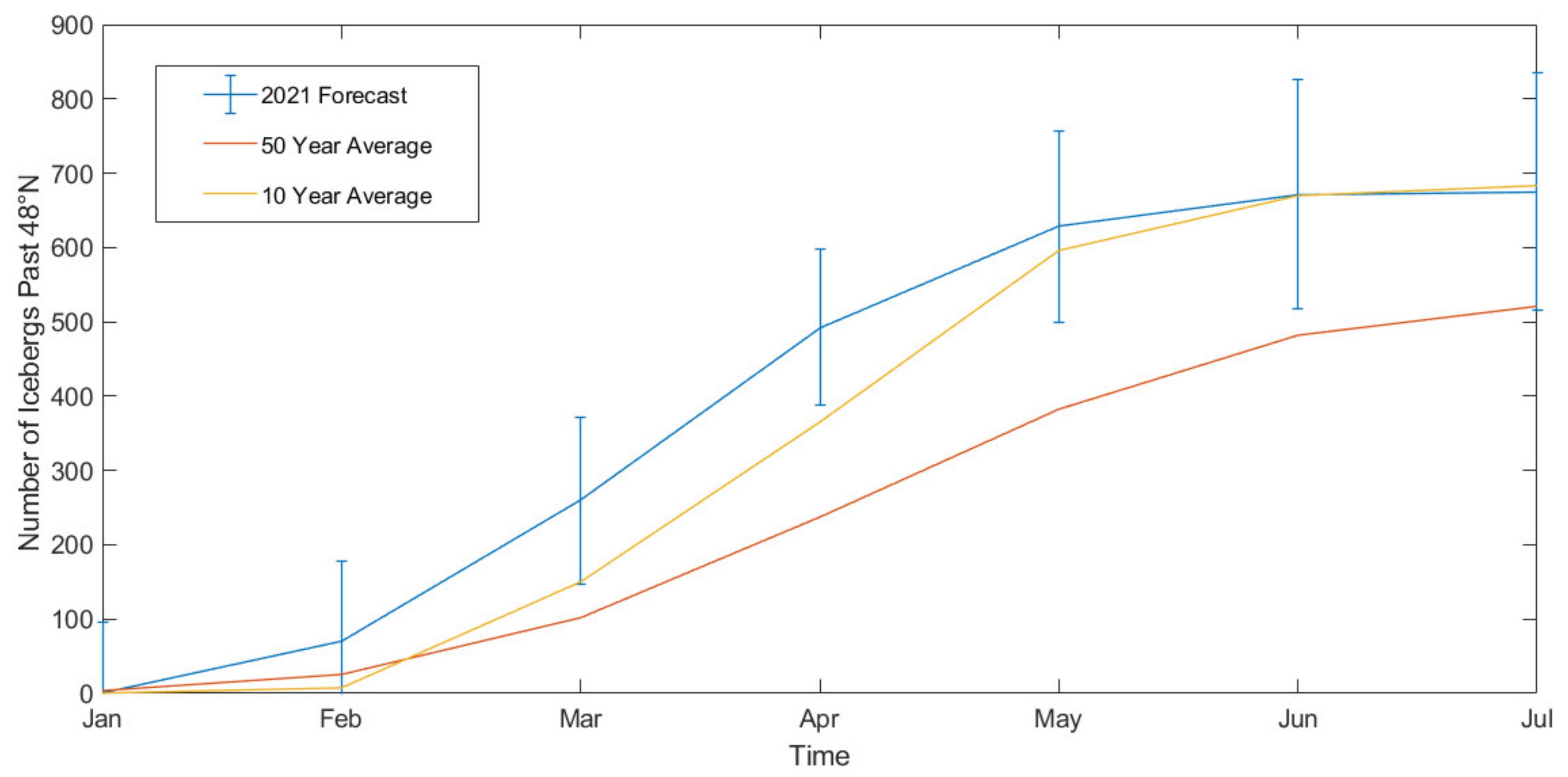
The predicted monthly cumulative totals can be seen in Figure 7, along with the average iceberg numbers for the last 10 and 50 years. The plot shows a steady increase in iceberg numbers over the years, with the greatest increase in the spring months. The 2021 forecast fits quite closely to the 10-year average, although with an earlier than normal peak rate of change, probably by April. Using the previous WERR model from [7], with the original training set, the forecast would have been 551 ± 297 icebergs, which would also predict a medium year.
3.4.2. Properties of the Machine Learning Models
Table 3 shows all combinations of the four machine learning outputs that have been predicted or observed in the testing period (1931–2017). In the Table 3 format ([I48N, RoC, peak month, number of peaks]), the 2021 forecast is [1,0,1,1]. This combination was previously observed twice; however, it is rarely a predicted combination, only appearing once in the Linear SVM outputs and never in the Linear Discriminant or the Quadratic SVM. The most common predicted outputs for each machine learning tool, respectively, are: [1,0,2,1], [1,0,2,1], and [0,0,2,1]. The most common observed combinations are [0,0,2,1] and [1,1,1,1]. The similarity in the predicted outcomes is consistent with observed results, in that one peak in May (e.g., [x,x,2,x]) is a common scenario. Likewise, one peak in April ([x,x,1,x]) is also often predicted, as in the second common observed combination. However, it is notable that there is a wider range of observed combinations (44) than any of the models predict (43, 34, and 39, respectively). The Linear Discriminant Model appears to best reflect the range of observed combinations, and also has a similar distribution across the structure given in Table 3.
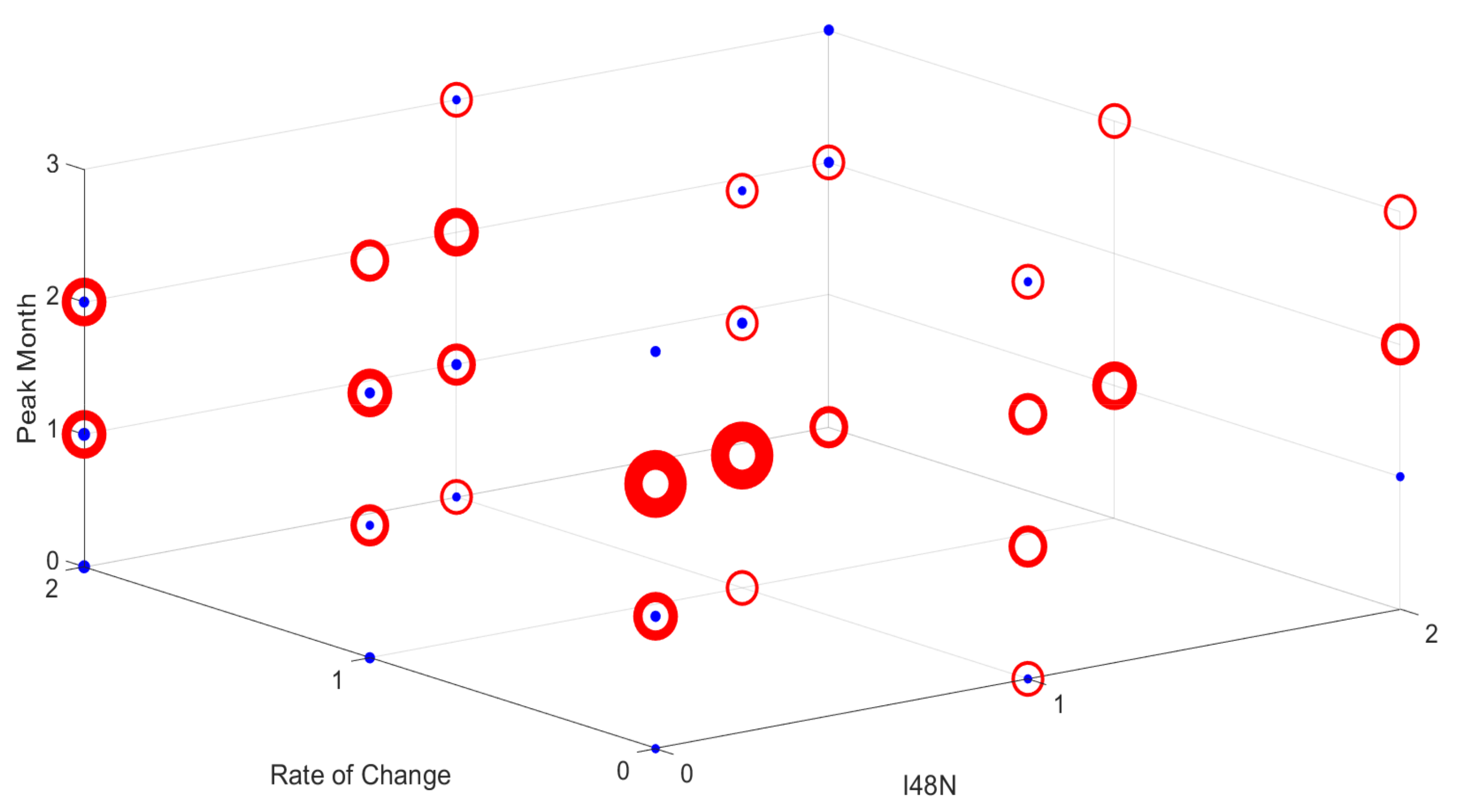
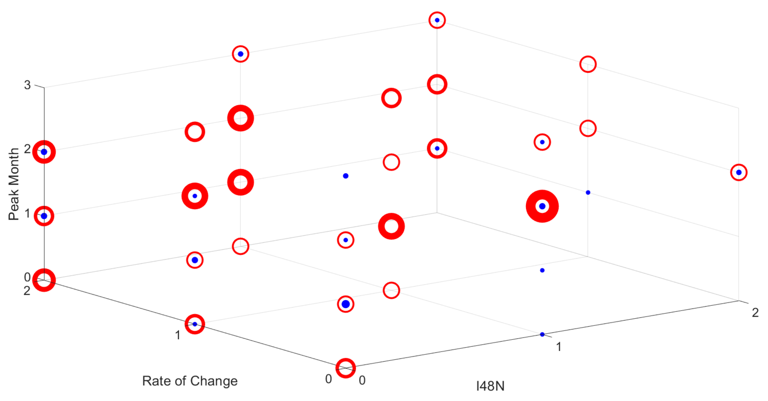
Figure 8 attempts to show in another, more graphical way, the common patterns in the observed combinations. This clearly shows that one peak (the red circles) is significantly more common than multiple peaks (in blue). The plot also shows that the majority of observed combinations have a low or medium I48N and a peak month of April or May. This seems sensible, as the average I48N has been increasing over the last century, and the training period is 1931 to 2017. Also, as previously mentioned, the peak month is usually April or May. Figure 9 shows, for comparison, the Linear Discriminant model distribution which most resembles the observed results. In general, the clustering occurs at similar locations but with the main differences at times of low rate of change. The model is also more likely to predict multiple peaks; however, as previously stated, the observational results may be under-representing this aspect. For reference, the 3D scatter plots of the Linear and Quadratic SVM models have been included in the supplementary material as Figures S5 and S6.
Another question regarding how well the machine learning models perform relative to the observed states is how well they do overall for each measure. Table 4 attempts to show this, through a comparison of the means and standard deviation of the various models compared to observations. The prediction of the number of peaks was excluded here as there are only two possible outcomes, and it can be seen from Figure 8 and Figure 9 that one peak is overwhelmingly dominant. Table 4 shows that the Linear Discriminant outputs have the most similar distribution to the observed results, with a very small net difference across all three measures. The Linear Discriminant model’s mean is best for two of the three measures (I48N and rate of change), and its standard deviation is best for all of the measures.
A final aspect of the machine learning models examined here is how successful the models are in predicting individual combinations for specific years. Table 3 showed that the Linear Discriminant Model had almost as many outcomes as in the observations, therefore the question is how this links to successful predictions. The successfully predicted combinations from the testing period of 1931–2017 can be seen in Table 5. Random chance suggests that only 1.36% of the 86 outcomes, or just one, would be expected to be predicted by a model if there were no skill in the models. However, 10 of the 44 observed combinations were successfully predicted by one or another of the models. One common combination, [0,0,2,1], which represents a low iceberg year, with a low rate of change and one peak in May, was correctly predicted multiple times. Each of the models showed levels of skill, with five, five, and nine successful predictions for the Linear Discriminant, Linear SVM, and Quadratic SVM models, respectively. Overall, Table 5 shows that the Quadratic SVM approach is the most likely to predict the entire combination, with the fewest “false alarms”. However, as even this tool successfully predicted only just over 10% of the years’ ice states exactly, it shows that assessment of likely iceberg season risk remains exploratory. Overall, the three machine learning models help to build a more comprehensive practical idea of iceberg conditions in a given year, rather than just predicting a final total.
3.4.3. The Machine Learning Forecast for 2021
All three machine learning models predict one significant peak in iceberg number and a medium iceberg year for 2021. There is more variability in the peak month prediction, where the models predict either 3 (June onwards) or 1 (April). However, as this measure has four possible outcomes, it naturally has the lowest accuracy; it also has the lowest skill level (see Table 1). As two models predict a peak in April and, as one of these, the Quadratic SVM, has the highest accuracy, the forecast is for the peak month to occur in April. For the final new measure, two models predict a low rate of change and one (Linear Discriminant) predicts a medium rate of change. This combination ([1,0,1,1]) is observationally possible. However, the more common predicted pattern similar to this would be one with a May peak ([1,0,2,1]). All model predictions for the 2021 iceberg season can be seen in Table 6.
From Table 6 it can be seen that, while the two SVM models agree on the 2021 forecast, the Linear Discriminant model is predicting a later peak, from June onwards, and a medium rate of change. This would produce a combination of [1,1,3,1], which has been observed once, and predicted by the Linear Discriminant model unsuccessfully twice. While the Linear Discriminant model has the most similar distribution to the observed results, the Quadratic SVM has greater accuracy in predicting the peak month. It also has the same accuracy, but with slightly more error, for the rate of change prediction. As both SVM models agree on the forecast, this has been the one selected.
Overall, the forecast is for one peak in iceberg numbers to occur in April, with a low rate of change, in a medium iceberg year. Therefore, the machine learning aspect agrees with the WERR prediction, that the 2021 ice season will be ‘medium’, with one peak in April.
3.4.4. Mid Season Forecast Update
Mid-season iceberg numbers south of the 48th parallel suggest that the 2021 season will be an extremely low iceberg year, with no icebergs recorded crossing 48° N up to mid-May. It is worth noting that such an extreme iceberg year, while not unknown, would always be extremely difficult to predict, as all prediction tools assume a non-zero iceberg flux across 48° N at some point in each year. Nevertheless, from the IIP daily charts, it can be seen that a wave of icebergs approached, but did not cross, 48° N in April. This suggests that although the peak southward iceberg flux occurred in April, as predicted, no iceberg actually entered the count zone. Also, from the decline in iceberg numbers further north off Labrador in May IIP charts, it seems unlikely that a late (June onwards) peak will occur.
4. Discussion and Conclusions
This paper presents a new machine learning approach to forecasting iceberg behaviour in the North West Atlantic. The addition of these machine learning models to an existing and updated control systems forecast has been done to supplement the WERR result and to try to predict more detailed and practically useful aspects of iceberg behaviour in the forthcoming ice year. The flexibility of the machine learning tools allows for a prediction of practically any quantity, restricted only by the available data. The four new measures in this paper were selected after end-user feedback from the IIP that these forecast aspects would be of interest for monitoring purposes. The machine learning models themselves were selected due to their established success in classification tasks in the environmental sector [13]; however, as this paper presents a new application of these models, future work may focus on optimizing the selection of machine learning approaches to achieve the best prediction performance in this field.
The WERR model forecast has been released to the IIP operationally every year since 2018, and two of the machine learning predictions—I48N and the rate of change—were also provided for the 2020 season. However, the 2021 ice season is the first to present all of the new measures and the WERR forecast. This combined 2021 iceberg forecast is for a medium iceberg year, with a single peak in April and a low rate of change, although as of the time of writing, 2021 looks likely to be an extreme year with no icebergs travelling south of 48N between March and mid-May, and therefore is effectively unforecastable by our approaches.
Analysis of the machine learning models shows that the I48N prediction is the most skillful, reflected in the accuracy, F1 score, and the confusion matrices provided in the Supplementary Materials. The other measures are more experimental; however, they still show respectable performance levels that provide a firm basis for improvement. Future forecasts would attempt to add confidence to the prediction by utilising the combination approach further. This could reduce the risk of one component disrupting the overall forecast, notably concerning the number of peaks and the peak month prediction. These have the lowest skill of the four measures and are therefore where future algorithm development should be focused. It would also be beneficial to further define the procedure for when the models disagree. Currently, this is done by using the most common prediction of the three; however, if the Linear Discriminant model proves to be the best fit, this model should be prioritised.
Despite the probable exceptional nature of the 2021 season, over the last century the average number of icebergs in a season has been increasing. It can be seen in Figure 7 that the average I48N for the last 10 years is significantly higher than for the last 50 years. The IIP are also aware of this trend, and have variable definitions for a high, low, or medium year, depending on the year in question (an extreme year before 1945 was for more than 844 icebergs). Sea ice extent has also been gradually decreasing, allowing shipping further north. While iceberg detection methods have greatly improved over the last century, so too has iceberg risk. Therefore, there is real practical application in long term iceberg warning. A combined forecast of iceberg severity gives the shipping industry time to adjust routes and departure times to avoid regions of high iceberg density. While this work is not currently at a stage to be crucial to the shipping sector, it shows both the predictive capacity of these machine learning tools in an area of high natural variability, and is of interest to the IIP in their continued role patrolling the region.
Supplementary Materials
The following are available online at https://0-www-mdpi-com.brum.beds.ac.uk/article/10.3390/su13147705/s1, Table S1: The ensemble of WERR Models used for the 2021 forecast. Figure S1: Showing the confusion matrices for the rate of change prediction. Figure S2: the confusion matrices for the number of peaks prediction. Figure S3: Showing the confusion matrices for the I48N prediction. Figure S4: Showing the confusion matrices for the peak month prediction. Figure S5: Plot of the linear SVM combinations from the testing period of 1931–2017. Figure S6: Plot of the quadratic SVM combinations from the testing period of 1931–2017.
Author Contributions
Conceptualization, G.R.B., J.B.R. and Y.Z.; methodology, J.B.R. and Y.Z.; software, J.B.R.; validation, J.B.R. and G.R.B.; formal analysis J.B.R. and G.R.B.; resources, E.H. and J.B.R.; writing—original draft preparation, J.B.R.; writing—review and editing, G.R.B., J.B.R., Y.Z. and E.H.; visualization, J.B.R. and Y.Z.; supervision, G.R.B. and Y.Z.; project administration, G.R.B.; funding acquisition, G.R.B. All authors have read and agreed to the published version of the manuscript.
Funding
The team behind the forecast was funded by insurance firm AXA XL’s Ocean Risks Scholarships programme.
Institutional Review Board Statement
Not applicable.
Data Availability Statement
The data sources are included in Section 2.1, and the ensemble WERR models are contained in the Supplementary Information.
Acknowledgments
E.H. acknowledges ECMWF for use of ERA-5 reanalysis data.
Conflicts of Interest
The authors declare no conflict of interest.
References
- Hanna, E.; Pattyn, F.; Navarro, F.; Favier, V.; Goelzer, H.; van den Broeke, M.R.; Vizcaino, M.; Whitehouse, P.L.; Ritz, C.; Bulthius, K.; et al. Mass balance of the ice sheets and glaciers—Progress since AR5 and challenges. Earth Sci. Rev. 2020, 201, 102976. [Google Scholar] [CrossRef]
- Hill, B.T. Database of Ship Collisions with Icebergs; Institute for Marine Dynamics: St. John’s, NL, Canada, 2000. [Google Scholar]
- Bigg, G.R.; Billings, S.A. The iceberg risk in the Titanic year of 1912: Was it exceptional? Significance 2014, 11, 6–10. [Google Scholar] [CrossRef]
- Murphy, D.L.; Cass, J.L. The International Ice Patrol, safeguarding life and property at sea. Coast Guard Proc. Mar. Safety Sec. Coun. 2012, 69, 13–16. [Google Scholar]
- Bigg, G.R.; Wei, H.; Wilton, D.J.; Zhao, Y.; Billings, S.A.; Hanna, E.; Kadirkamanathan, V. A century of variation in the dependence of Greenland iceberg calving on ice sheet surface mass balance and regional climate change. Proc. Roy. Soc. Ser. A 2014, 470, 20130662. [Google Scholar] [CrossRef] [PubMed] [Green Version]
- Zhao, Y.; Bigg, G.R.; Billings, S.A.; Hanna, E.; Sole, A.J.; Wei, H.; Kadirkamanathan, V.; Wilton, D.J. Inferring the variation of climatic and glaciological contributions to West Greenland iceberg discharge in the Twentieth Century. Cold Reg. Sci. Technol. 2016, 121, 167–178. [Google Scholar] [CrossRef] [Green Version]
- Zhao, Y.; Hanna, E.; Bigg, G.R.; Zhao, Y. Tracking nonlinear correlation for complex dynamic systems using a Windowed Error Reduction Ratio method. Complexity 2017, 8570720. [Google Scholar] [CrossRef] [Green Version]
- Bigg, G.R.; Zhao, Y.; Hanna, E. Forecasting the severity of the Newfoundland iceberg season using a control systems model. J. Oper. Oceanogr. 2021, 14, 24–36. [Google Scholar] [CrossRef]
- International Ice Patrol. Report of the International Ice Patrol in the North Atlantic Season of 2019; CG-188-74; U.S. Coast Guard: Washington, DC, USA, 2019. [Google Scholar]
- Hanna, E.; Huybrechts, P.; Cappelen, J.; Steffen, K.; Bales, R.C.; Burgess, E.; McConnell, J.R.; Steffensen, J.P.; Van den Broeke, M.; Wake, L.; et al. Greenland Ice Sheet surface mass balance 1870 to 2010 based on Twentieth Century Reanalysis, and links with global climate forcing. J. Geophys. Res. Atmos. 2011, 116, D24121. [Google Scholar] [CrossRef] [Green Version]
- Wilton, D.J.; Jowett, A.; Hanna, E.; Bigg, G.R.; van den Broeke, M.R.; Fettweis, X.; Huybrechts, P. High resolution (1 km), positive degree-day modelling of Greenland Ice Sheet Surface Mass Balance, 1870-2012 using reanalysis data. J. Glaciol. 2017, 63, 176–193. [Google Scholar] [CrossRef] [Green Version]
- Janssens, I.; Huybrechts, P. The treatment of meltwater retention in mass-balance parameterisation of the Greenland Ice Sheet. Ann. Glaciol. 2000, 31, 133–140. [Google Scholar] [CrossRef] [Green Version]
- Khondoker, M.; Dobson, R.; Skirrow, C.; Simmons, A.; Stahl, D. A comparison of machine learning methods for classification using simulation with multiple real data examples from mental health studies. Stat. Methods Med Res. 2016, 25, 1804–1823. [Google Scholar] [CrossRef] [PubMed] [Green Version]
- Fisher, R.A. The use of multiple measurements in taxonomic problems. Ann. Eugen. 1936, 7, 179–188. [Google Scholar] [CrossRef]
- Pham, B.T.; Prakash, I. Evaluation and comparison of LogitBoost Ensemble, Fisher’s Linear Discriminant Analysis, logistic regression and support vector machines methods for landslide susceptibility mapping. Geocarto Int. 2019, 34, 316–333. [Google Scholar] [CrossRef]
- AbuZeina, D.; Al-Anzi, F.S. Employing fisher discriminant analysis for Arabic text classification. Comp. Elec. Eng. 2018, 66, 474–486. [Google Scholar] [CrossRef]
- Hoang, N.D.; Bui, D.T. Predicting earthquake-induced soil liquefaction based on a hybridization of kernel Fisher discriminant analysis and a least squares support vector machine: A multi-dataset study. Bull. Eng. Geol. Env. 2018, 77, 191–204. [Google Scholar] [CrossRef]
- Kakhki, F.D.; Freeman, S.A.; Mosher, G.A. Evaluating machine learning performance in predicting injury severity in agribusiness industries. Saf. Sci. 2019, 117, 257–262. [Google Scholar] [CrossRef]
- Fathi, M.; Nemati, M.; Mohammadi, S.M.; Abbasi-Kesbi, R. A machine learning approach based on SVM for classification of liver diseases. Biomed. Eng. Appl. Basis Commun. 2020, 32, 2050018. [Google Scholar] [CrossRef]
- Obaid, O.I.; Mohammed, M.A.; Ghani, M.K.A.; Mostafa, A.; Taha, F. Evaluating the performance of machine learning techniques in the classification of Wisconsin Breast Cancer. Int. J. Eng. Technol. 2018, 7, 160–166. [Google Scholar]
- Khan, T.A.; Alam, M.; Kadir, K.; Shahid, Z.; Mazliham, M.S. A comparison review based on classifiers and regression models for the investigation of flash floods. Int. J. Adv. Comp. Sci. Appl. 2019, 10, 352–359. [Google Scholar] [CrossRef]
- Chokey, T.; Jain, S. Quality Assessment of crops using machine learning techniques. In Proceedings of the 2019 Amity International Conference on Artificial Intelligence, Dubai, United Arab Emirates, 4–6 February 2019; pp. 259–263. [Google Scholar]
- Bhuvaneswari, P.; Kumar, J.S. Support vector machine technique for EEG signals. Int. J. Comput. Appl. 2013, 63, 1–5. [Google Scholar] [CrossRef]
Figure 1.
Map showing the major iceberg paths in the region, with mean April sea ice extent represented by the dashed line. The dotted line estimates 48° N, while the ‘+’ shows the location of the sinking of the Titanic. (Reprinted with Open Access CC BY permission, from [8]).
Figure 1.
Map showing the major iceberg paths in the region, with mean April sea ice extent represented by the dashed line. The dotted line estimates 48° N, while the ‘+’ shows the location of the sinking of the Titanic. (Reprinted with Open Access CC BY permission, from [8]).

Figure 2.
Plot of the average number of icebergs past 48° N in each month, from 1950 to 2020.

Figure 3.
Plot of the cumulative iceberg numbers south of 48° N in the last 50 years. 2019 and 2017 have been highlighted (in magenta and blue, respectively) as they show clearly the characteristics of each new measure for prediction within the context of an iceberg season.
Figure 3.
Plot of the cumulative iceberg numbers south of 48° N in the last 50 years. 2019 and 2017 have been highlighted (in magenta and blue, respectively) as they show clearly the characteristics of each new measure for prediction within the context of an iceberg season.

Figure 4.
Visualization of the optimal linear hyperplane (solid line) that classifies the data into two classes (diamonds and stars) in a support vector machine approach; inspired by [23]. The support vectors are shown by the dashed lines.
Figure 4.
Visualization of the optimal linear hyperplane (solid line) that classifies the data into two classes (diamonds and stars) in a support vector machine approach; inspired by [23]. The support vectors are shown by the dashed lines.

Figure 5.
Plot of WERR model fit vs. observed data for the latest 30-year window model. Upper panel shows the monthly fit, while the lower panel shows the annual total produced by the model, compared to observations.
Figure 5.
Plot of WERR model fit vs. observed data for the latest 30-year window model. Upper panel shows the monthly fit, while the lower panel shows the annual total produced by the model, compared to observations.

Figure 6.
Plot of the monthly time series data of SMB, LSST, and NAO that was used for the WERR ensemble.
Figure 6.
Plot of the monthly time series data of SMB, LSST, and NAO that was used for the WERR ensemble.

Figure 7.
Plot of the 2021 iceberg forecast, including the average number of icebergs past 48° N by the end of July in the last 10 and 50 years.
Figure 7.
Plot of the 2021 iceberg forecast, including the average number of icebergs past 48° N by the end of July in the last 10 and 50 years.

Figure 8.
Plot of the observed combinations from the testing period of 1931–2017, where I48N, the rate of change, and the peak month are marked on the axis. A red circle corresponds to one peak, while blue represents multiple peaks. The larger the circle, the more times that combination has occurred.

Figure 9.
Plot of the Linear Discriminant combinations from the testing period of 1931–2017, where I48N, the rate of change, and the peak month are marked on the axis. A red circle corresponds to one peak, while blue represents multiple peaks. The larger the circle, the more times that combination has occurred.


Table 1.
Showing the accuracy, F1 score, and root mean squared error (RMSE) of the various machine learning models over the trial period of 1931–2017. The last row shows the mean skill level for each variable predicted, defined as the mean model accuracy/(expected random accuracy).
Table 1.
Showing the accuracy, F1 score, and root mean squared error (RMSE) of the various machine learning models over the trial period of 1931–2017. The last row shows the mean skill level for each variable predicted, defined as the mean model accuracy/(expected random accuracy).
| I48N Annual Total | Rate of Change | Number of Peaks | Peak Month | |||||||||
|---|---|---|---|---|---|---|---|---|---|---|---|---|
| Accuracy (%) | F1 | RMSE | Accuracy (%) | F1 | RMSE | Accuracy (%) | F1 | RMSE | Accuracy (%) | F1 | RMSE | |
| Linear Discriminant | 54.6512 | 0.66 | 0.7924 | 41.8605 | 0.52 | 1 | 55.814 | 0.77 | 0.6647 | 26.7442 | 0.54 | 1.3118 |
| Linear SVM | 50 | 0.70 | 0.8627 | 37.2093 | 0.62 | 1.023 | 56.9767 | 0.78 | 0.6559 | 26.7442 | 0.59 | 1.2152 |
| Quadratic SVM | 50 | 0.71 | 0.9022 | 41.8605 | 0.59 | 1.0173 | 60.4651 | 0.77 | 0.6288 | 30.2326 | 0.52 | 1.3725 |
| Mean Skill level | 1.55 | 1.21 | 1.16 | 1.12 | ||||||||
Table 2.
Showing the machine learning hindcasts (in order Linear Discriminant, Linear SVM and Quadratic SVM) separated by commas. The observed class is shown in bold.
Table 2.
Showing the machine learning hindcasts (in order Linear Discriminant, Linear SVM and Quadratic SVM) separated by commas. The observed class is shown in bold.
| Year | I48N | RoC | Peak Month | No. of Peaks | ||||
|---|---|---|---|---|---|---|---|---|
| 2017 | 1,1,1 | 1 | 1,1,1 | 0 | 2,2,2 | 1 | 1,1,1 | 1 |
| 2018 | 1,1,1 | 0 | 0,0,1 | 1 | 2,2,1 | 0 | 2,2,1 | 2 |
| 2019 | 2,2,2 | 2 | 0,0,1 | 1 | 1,1,2 | 2 | 1,1,1 | 2 |
| 2020 | 0,0,1 | 0 | 1,1,0 | 2 | 2,2,2 | 1 | 1,1,1 | 1 |
Table 3.
Machine learning output combinations over 1931–2017. Here the order is: I48N, rate of change (RoC), the peak month, and the number of peaks. Therefore, a combination of [0,0,2,1] is for a low ice year, with a low rate of change, and one significant peak in May. The last row in each set shows the sub-column totals, with the total sub-set of combinations in brackets in the first column.
| Combinations with 0 I48N | Number of Repetitions | Combinations with 1 I48N | Number of Repetitions | Combinations with 2 I48N | Number of Repetitions | |
|---|---|---|---|---|---|---|
| Observed Combinations | [0,0,2,1] | 6 | [1,1,1,1] | 6 | [2,1,1,1] | 3 |
| [0,2,1,2] | 3 | [1,2,2,1] | 3 | [2,0,2,1] | 2 | |
| [0,1,2,1] | 3 | [1,1,2,2] | 2 | [2,2,3,2] | 2 | |
| [0,2,0,2] | 3 | [1,0,2,1] | 2 | [2,2,0,1] | 2 | |
| [0,2,1,1] | 3 | [1,2,1,2] | 2 | [2,2,2,2] | 2 | |
| [0,2,2,1] | 3 | [1,2,1,1] | 2 | [2,2,2,1] | 1 | |
| [0,0,1,1] | 3 | [1,0,1,1] | 2 | [2,1,3,1] | 1 | |
| [0,0,3,2] | 2 | [1,1,0,1] | 1 | [2,0,1,2] | 1 | |
| [0,1,1,1] | 2 | [1,1,2,1] | 1 | [2,0,3,1] | 1 | |
| [0,1,0,2] | 2 | [1,1,3,2] | 1 | |||
| [0,0,1,2] | 2 | [1,0,3,1] | 1 | |||
| [0,1,3,1] | 2 | [1,2,0,2] | 1 | |||
| [0,1,2,2] | 2 | [1,2,3,2] | 1 | |||
| [0,2,2,2] | 2 | [1,0,3,2] | 1 | |||
| [0,1,1,2] | 1 | [1,0,0,2] | 1 | |||
| [0,0,0,2] | 1 | [1,2,0,1] | 1 | |||
| [1,0,0,1] | 1 | |||||
| [1,2,3,1] | 1 | |||||
| [1,1,3,1] | 1 | |||||
| Total (44) | 16 | 40 | 19 | 31 | 9 | 15 |
| Linear Discriminant Output Combinations | [0,0,1,2] | 5 | [1,0,2,1] | 6 | [2,2,2,1] | 2 |
| [0,1,2,1] | 4 | [1,2,2,1] | 4 | [2,0,2,2] | 2 | |
| [0,2,0,1] | 3 | [1,1,1,1] | 4 | [2,2,1,1] | 2 | |
| [0,2,2,1] | 3 | [1,2,1,1] | 4 | [2,2,3,2] | 1 | |
| [0,2,2,2] | 3 | [1,0,2,2] | 3 | [2,2,1,2] | 1 | |
| [0,1,1,2] | 3 | [1,1,3,1] | 2 | [2,1,1,2] | 1 | |
| [0,2,1,2] | 3 | [1,2,3,2] | 2 | [2,2,3,1] | 1 | |
| [0,0,3,2] | 2 | [1,0,3,2] | 1 | [2,0,2,1] | 1 | |
| [0,2,1,1] | 2 | [1,0,0,2] | 1 | [2,1,3,1] | 1 | |
| [0,1,2,2] | 2 | [1,0,1,2] | 1 | [2,1,2,1] | 1 | |
| [0,1,3,1] | 2 | [1,2,0,1] | 1 | |||
| [0,1,0,1] | 2 | [1,1,0,1] | 1 | |||
| [0,0,2,1] | 1 | [1,2,3,1] | 1 | |||
| [0,0,1,1] | 1 | [1,1,2,1] | 1 | |||
| [0,1,0,2] | 1 | [1,0,3,1] | 1 | |||
| [0,1,1,1] | 1 | |||||
| [0,0,2,2] | 1 | |||||
| [0,2,0,2] | 1 | |||||
| Total (43) | 18 | 40 | 15 | 33 | 10 | 13 |
| Linear SVM Output Combinations | [0,0,2,1] | 5 | [1,0,2,1] | 6 | [2,2,1,2] | 3 |
| [0,1,2,1] | 5 | [1,2,2,1] | 4 | [2,1,2,1] | 2 | |
| [0,0,1,2] | 5 | [1,1,2,1] | 4 | [2,0,3,1] | 2 | |
| [0,2,2,1] | 5 | [1,0,2,2] | 3 | [2,1,1,2] | 1 | |
| [0,2,1,1] | 5 | [1,2,0,1] | 3 | [2,2,2,1] | 1 | |
| [0,0,2,2] | 3 | [1,2,1,1] | 2 | [2,1,2,1] | 1 | |
| [0,1,1,1] | 3 | [1,1,1,1] | 2 | |||
| [0,2,1,2] | 3 | [1,0,1,2] | 2 | |||
| [0,1,2,2] | 2 | [1,1,3,2] | 1 | |||
| [0,1,1,2] | 2 | [1,2,3,2] | 1 | |||
| [0,2,0,1] | 2 | [1,0,1,1] | 1 | |||
| [0,2,2,2] | 2 | [1,2,1,2] | 1 | |||
| [0,0,1,1] | 1 | [1,0,3,1] | 1 | |||
| [0,2,3,1] | 1 | |||||
| [0,1,0,1] | 1 | |||||
| Total (34) | 15 | 45 | 13 | 31 | 6 | 10 |
| Quadratic SVM Output Combinations | [0,0,2,1] | 7 | [1,1,2,1] | 5 | [2,2,2,2] | 2 |
| [0,2,2,1] | 5 | [1,2,0,1] | 3 | [2,2,0,2] | 2 | |
| [0,0,1,2] | 4 | [1,2,1,1] | 3 | [2,0,3,1] | 1 | |
| [0,2,1,2] | 4 | [1,2,2,1] | 2 | [2,2,0,1] | 1 | |
| [0,1,1,1] | 4 | [1,0,2,1] | 2 | [2,1,2,1] | 1 | |
| [0,0,0,1] | 3 | [1,1,2,2] | 2 | |||
| [0,1,2,2] | 3 | [1,1,1,1] | 2 | |||
| [0,2,1,1] | 3 | [1,2,1,2] | 2 | |||
| [0,2,2,2] | 3 | [1,2,3,1] | 2 | |||
| [0,2,3,2] | 2 | [1,2,2,2] | 1 | |||
| [0,0,2,2] | 2 | [1,0,1,2] | 1 | |||
| [0,1,2,1] | 2 | [1,2,0,2] | 1 | |||
| [0,2,0,1] | 2 | [1,1,0,2] | 1 | |||
| [0,0,3,1] | 1 | [1,0,2,2] | 1 | |||
| [0,1,1,2] | 1 | [1,0,0,1] | 1 | |||
| [0,0,3,2] | 1 | |||||
| [0,1,0,1] | 1 | |||||
| [0,1,0,2] | 1 | |||||
| [0,2,3,1] | 1 | |||||
| Total (39) | 19 | 50 | 15 | 29 | 5 | 7 |
Table 4.
Distribution of combinations. The table shows the mean and standard deviation of the predicted and observed I48N, rate of change (RoC), and the peak month over the trial period of 1931–2017. Also shown is the total difference between the unweighted means of each of the three quantities predicted and the observations. Models closest to observations are shown in bold for each measure.
| Observed/Model | I48N | RoC | Peak Month | Total Diff. from Obs. |
|---|---|---|---|---|
| Observed | 0.71 ± 0.75 | 1.07 ± 0.82 | 1.51 ± 0.94 | |
| Linear Discriminant | 0.69 ± 0.72 | 1.06 ± 0.85 | 1.58 ± 0.91 | 0.10 |
| Linear SVM | 0.58 ± 0.69 | 0.99 ± 0.87 | 1.50 ± 0.73 | 0.22 |
| Quadratic SVM | 0.50 ± 0.65 | 1.16 ± 0.85 | 1.41 ± 0.90 | 0.40 |
Table 5.
Showing all the successfully predicted combinations over the trial period of 1931–2017, with the number of times this occurred compared to how many times it was predicted. In the list of successful combinations, the number in brackets gives the number of years in which this combination was found.
| Number of Successful Prediction | Total Number of Predictions | ||||||||
|---|---|---|---|---|---|---|---|---|---|
| Successful Combination | Linear Discriminant | Linear SVM | Quadratic SVM | Linear Discriminant | Linear SVM | Quadratic SVM | |||
| 0 | 0 | 1 | 2 (2) | 1 | 1 | 1 | 5 | 5 | 4 |
| 0 | 0 | 2 | 1 (6) | 1 | 2 | 2 | 1 | 5 | 7 |
| 0 | 1 | 1 | 2 (1) | 1 | 0 | 0 | 3 | 2 | 1 |
| 0 | 1 | 2 | 1 (3) | 0 | 1 | 1 | 4 | 5 | 2 |
| 0 | 2 | 1 | 1 (3) | 0 | 0 | 1 | 2 | 5 | 3 |
| 0 | 2 | 2 | 1 (3) | 0 | 0 | 1 | 3 | 5 | 5 |
| 1 | 0 | 2 | 1 (2) | 1 | 1 | 1 | 6 | 6 | 2 |
| 1 | 2 | 1 | 1 (2) | 1 | 0 | 0 | 4 | 2 | 3 |
| 1 | 2 | 2 | 1 (3) | 0 | 0 | 1 | 4 | 4 | 2 |
| 2 | 2 | 2 | 2 (2) | 0 | 0 | 1 | 0 | 0 | 2 |
| Total | 5 | 5 | 9 | 32 | 39 | 31 | |||
Table 6.
The predictions for the 2021 iceberg season, for the different machine learning models.
| Model | I48N | RoC | Peak Month | No. of Peaks |
|---|---|---|---|---|
| Linear Discriminant | Medium | Medium | June onwards | One |
| Linear SVM | Medium | Low | April | One |
| Quadratic SVM | Medium | Low | April | One |
Publisher’s Note: MDPI stays neutral with regard to jurisdictional claims in published maps and institutional affiliations. |
© 2021 by the authors. Licensee MDPI, Basel, Switzerland. This article is an open access article distributed under the terms and conditions of the Creative Commons Attribution (CC BY) license (https://creativecommons.org/licenses/by/4.0/).
Share and Cite
MDPI and ACS Style
Ross, J.B.; Bigg, G.R.; Zhao, Y.; Hanna, E. A Combined Control Systems and Machine Learning Approach to Forecasting Iceberg Flux off Newfoundland. Sustainability 2021, 13, 7705. https://0-doi-org.brum.beds.ac.uk/10.3390/su13147705
AMA Style
Ross JB, Bigg GR, Zhao Y, Hanna E. A Combined Control Systems and Machine Learning Approach to Forecasting Iceberg Flux off Newfoundland. Sustainability. 2021; 13(14):7705. https://0-doi-org.brum.beds.ac.uk/10.3390/su13147705
Chicago/Turabian StyleRoss, Jennifer B., Grant R. Bigg, Yifan Zhao, and Edward Hanna. 2021. "A Combined Control Systems and Machine Learning Approach to Forecasting Iceberg Flux off Newfoundland" Sustainability 13, no. 14: 7705. https://0-doi-org.brum.beds.ac.uk/10.3390/su13147705
Note that from the first issue of 2016, this journal uses article numbers instead of page numbers. See further details here.