
An Importance Sampling Framework for Time-Variant Reliability Analysis Involving Stochastic Processes


School of Mechanical Engineering & Automation, Northeastern University, Shenyang 110819, China
*
Author to whom correspondence should be addressed.
Sustainability 2021, 13(14), 7776; https://0-doi-org.brum.beds.ac.uk/10.3390/su13147776
Submission received: 9 March 2021
/
Revised: 1 July 2021
/
Accepted: 8 July 2021
/
Published: 12 July 2021
(This article belongs to the Special Issue Reliability and Optimization for Engineering Design)
Abstract
:In recent years, methods were proposed so as to efficiently perform time-variant reliability analysis. However, importance sampling (IS) for time-variant reliability analysis is barely studied in the literature. In this paper, an IS framework is proposed. A multi-dimensional integral is first derived to define the time-variant cumulative probability of failure, which has the similar expression to the classical definition of time-invariant failure probability. An IS framework is then developed according to the fact that time-invariant random variables are commonly involved in time-variant reliability analysis. The basic idea of the proposed framework is to simultaneously apply time-invariant IS and crude Monte Carlo simulation on time-invariant random variables and stochastic processes, respectively. Thus, the probability of acquiring failure trajectories of time-variant performance function is increased. Two auxiliary probability density functions are proposed to implement the IS framework. However, auxiliary PDFs available for the framework are not limited to the proposed two. Three examples are studied in order to validate the effectiveness of the proposed IS framework.
1. Introduction
Most mechanical structures and systems are vulnerable against uncertainties, such as loads and material properties. Reliability analysis provides an appropriate framework to evaluate the probability that a structure or system successfully performs its intended functions over a time interval of interest without failures, considering various forms of uncertainties [1]. Over the past decades, time-invariant reliability analysis methods have been well developed, e.g., analytical methods [2] and simulation-based methods [3,4]. Since dynamic or time-variant uncertainties are often involved, mechanical structures and systems are commonly related to performance degradation, and time-invariant methods cannot be directly used to perform time-variant reliability analysis. Time-variant reliability analysis has gained much attention as a method to deal with the issue. Methods for time-variant reliability analysis in the literature can be roughly summarized into two categories: first-crossing-based methods and extreme-value-based methods.
After the well-known Rice formula was proposed, first-crossing-based methods gained much attention [5,6,7,8]. This kind of method concentrates on calculating the probability that the out-crossing event occurs for the first time in a predefined time interval. The out-crossing event shows that the performance value of a structure exceeds a predefined threshold. With the assumption that out-crossing events are mutually independent when they occur, first-crossing-based methods approximate the cumulative probability of failure using an integration of the out-crossing rate which represents the mean number of out-crossing events per unit of time. Accordingly, calculating the out-crossing rate is vital to first-crossing-based methods. For instance, Renaud et al. [6] presented a PHI2 method which calculated the out-crossing rate by solving a two-component parallel system reliability problem. Sudret [9] proposed an improved version of PHI2 by providing analytical expressions of out-crossing rate. However, the independence assumption may lead to large errors in engineering when out-crossing events are strongly dependent. To address the deficiency, Hu and Du [10] relaxed the assumption using the concept of joint crossing rate, and Yu et al. [11] proposed an approximation of the first-crossing probability density function (PDF) method to avoid direct calculations of the out-crossing rate. The performance of a mechanical structure is commonly a stochastic process because of time-variant uncertainties and uncertainty propagation. Zhang et al. [12] first transformed the time-variant performance into an equivalent Gaussian process and then used crude Monte Carlo simulation (MCS) to calculate the cumulative probability of failure. In addition, composite limit state [13,14], failure process decomposition [15], total probability theorem [16] and stochastic process discretization [17,18] have also been proposed to evaluate the cumulative probability of failure.
It is acknowledged that a mechanical structure fails if the extreme value of its time-variant performance over the time interval of interest exceeds a predefined threshold. Therefore, the extreme value is the primary focus of extreme-value-based methods. Hu and Du [19] proposed a sampling method to estimate the distribution of the extreme value of a stochastic process. Ping et al. [20] proposed an extreme-value event evolution method to obtain the time-variant failure probability corresponding to arbitrary time interval and arbitrary failure threshold. Yu et al. [21] combined the extreme-value moment method and improved the maximum entropy method to address time-variant problems involving multiple failure modes and temporal parameters. In recent years, surrogate models have been adopted to improve the computational efficiency of extreme-value-based methods [22,23,24]. For instance, Hu et al. [25] proposed a single-loop Kriging (SILK) to reduce computational effort of the double-loop procedure [26,27]. In SILK, the Kriging model is adaptively refined based on the learning function U [28] that was originally developed for time-invariant reliability analysis. Considering that the acquisition of failure information may be difficult, Zafar and Wang [29] used transfer learning and the Kriging model to overcome this issue. Lara et al. [23] used polynomial chaos expansion to construct an approximate expression of a time-consuming model and then applied crude MCS on the surrogate model to obtain the cumulative probability of failure. Compared with other methods, surrogate-model-based methods remarkably reduce the number of evaluations of time-consuming models.
The random simulation-based method is also a representative extreme-value-based method. Crude MCS directly generates random trajectories of time-variant performance function. The computational cost presents a major challenge for the application of crude MCS even though it is easy to implement. Therefore, it is often combined with other methods to evaluate time-variant probability of failure, such as surrogate-model-based methods and a part of first-crossing-based methods. A great amount of the literature in regards to crude MCS as the benchmark compares efficiency and accuracy of other methods [6,24,25,30]. Subset simulations (SS), such as Markov Chain Monte Carlo (MCMC), SS with splitting method [31,32] and SS with splitting and partitioning in time [33], are efficient methods for precisely evaluating time-variant probability of failure. However, they are developed to deal with dynamical systems subject to stochastic excitation, and not applicable to problems involving general stochastic process (e.g., Gaussian processes). To address time-variant reliability analysis involving stochastic processes, Du et al. [34] applied parallel SS which was first used to evaluate the failure probabilities of multiple time-invariant limit states, and proposed a method to determine the so-called principal variable.
Importance sampling (IS) techniques for time-variant reliability analysis are barely studied in the literature, whereas IS for time-invariant reliability analysis have been well developed [35,36]. This paper intends to fill the gap and propose an importance sampling framework for time-variant reliability analysis. The input variables of a time-variant performance function of a mechanical structure commonly contain both time-invariant random variables and stochastic processes. Performance values of the structure at different time instants are correlated, because they share the same time-invariant variables and realizations of stochastic processes at different instants are correlated with each other. Considering that applying IS on stochastic processes is difficult, the IS framework proposed in this paper applies time-invariant IS on the time-invariant random variables and samples random trajectories of stochastic processes according to crude MCS in order to generate more failure trajectories of time-variant performance function and enhance the computational efficiency of time-variant reliability analysis.
The remainder of this paper is organized as follows. Section 2.1 provides the problem statement of time-variant reliability analysis and Section 2.2 briefly introduces the crude MCS. The proposed IS framework is developed in Section 3.1, which is followed by two auxiliary PDFs in Section 3.2. The proposed framework is validated in Section 4. Section 5 is the conclusion.
2. Time-Variant Reliability Analysis and Crude MCS
2.1. Time-Variant Reliability Analysis
In engineering, the reliability of a mechanical structure or system generally degrades over its service time t. The performance function G(X, Z(t), t), also called limit state function, is commonly used to determine whether a structure or system can fulfill its intended functions under intended conditions. is the vector of random variables, collecting the time-invariant variables, e.g., geometric properties. represents the vector of stochastic processes, e.g., loadings and degradations in material properties. Failure occurs when the performance value is beyond a prescribed threshold. For simplicity, this paper defines the failure state as G(X,Z(t),t) ≤ 0. Therefore, the cumulative probability of failure associated with G(X, Z(t), t) can be expressed as:
where [t0, te] is the time interval of interest. is the probability operator and “” means “there exists”. It is worth noting that Pf,c(t0,te) is relatively different from the instantaneous probability of failure Pf,i(t) at time which has the following expression:
As illustrated in Section 1, estimating the probability defined by Equation (1) has received wide attention in the literature, and two categories of methods, i.e., first-crossing-based methods and extreme-value-based methods, have been proposed.
The former category focuses on calculating the out-crossing rate,
Sequentially, the cumulative probability of failure can be approximated by:
where Pf,i(t0) is the instantaneous probability of failure at the initial time instant t0. Out-crossing rate methods are developed under the assumption that out-crossing events are mutually independent. They may provide inaccurate results, especially when out-crossing events are strongly dependent.
Extreme-value-based methods are based on the fact that a failure event occurs when the minimum of G(X,Z(t),t) over [t0, te] is negative. The minimum of G(X,Z(t),t) relies on the realization of X and the trajectory of Z(t), so expansion techniques are essential to generate random trajectories of Z(t). Currently, the expansion optimal linear estimation method (EOLE) and Karhunen–Loève (KL) expansion are widely employed in the literature. In spite of their difference, both methods represent a stochastic process with a set of uncorrelated random variables. This section does not discuss which method is more suitable for discretizing a stochastic process and just assumes that the stochastic process Z(m)(t) is modeled by the random vector (m = 1, …, M2). The notation W is introduced to collect all the uncorrelated variables (I = 1, …, pm; m = 1, …, M2). Consequentially, the trajectory of Z(t) fully relies on the realization of random vector W. From the perspective of extreme-value-based methods, the cumulative probability of failure can be expressed as a formulation of a multi-dimensional integral:
where fX(x) and fW(w) are the joint PDFs of X and W, respectively. I(x,w) is the cumulative failure indicator defined as follows:
where z(t) (t0 ≤ t ≤ te) is the trajectory of Z(t) determined by w.
2.2. Crude Monte Carlo Simulation
Crude MCS is obviously the most robust method to estimate the cumulative probability of failure defined by Equation (3). It estimates using the expression below:
where and (n = 1, …, NMC), i.i.d. realizations of X and W, are generated according to fX(x) and fW(w), respectively.
The coefficient of variation of is:
where,
3. Importance Sampling for Time-Variant Reliability Analysis
For any x and w, there is a trajectory of G(X,Z(t),t) associated with them, and hundreds or even thousands of evaluations of the time-variant performance function are needed to determine the value of I(x,w). Moreover, crude MCS requires enormous trajectories of G(X,Z(t),t) to achieve a desired estimate of the cumulative failure probability. For example, to achieve a coefficient of variation close to 3%, about 10p+3 random trajectories are required to access a probability of 10−p. Therefore, regardless of whether crude MCS is used alone or is combined with a surrogate model, its computational cost is significantly high when is small. This section aims to propose a framework in order to reduce the size of random population.
3.1. The Importance Sampling Framework
IS methods to improve the efficiency of time-invariant reliability analysis have been extensively studied and adopted in the literature [37,38], e.g., those based on the most probable point (MPP) of failure and kernel-density-based IS methods. Their basic idea is to increase the probability that failure samples are generated by introducing an auxiliary density.
IS methods for time-variant reliability analysis are barely studied in the literature because stochastic processes are commonly involved in time-variant problems and IS is difficult to conduct on stochastic processes. According to Section 2.2, crude MCS for time-variant reliability analysis can be performed as follows: (1) generate random samples (n = 1, …, NMC) according to the joint PDF fX(x); (2) generate (n = 1, …, NMC) according to fW(w); (3) determine values of (n = 1, …, NMC) based on the combination ; (4) compute . In other words, the random realizations of X and W are separately generated in the procedure of crude MCS. Therefore, this paper conducts IS on the random vector X by introducing the basic idea of IS methods for time-invariant reliability analysis into time-variant reliability analysis. Equation (3) can be rewritten as follows:
where hX(x) is the auxiliary PDF this paper introduces. Sequentially, can be estimated as:
where and (n = 1, …, NIS) are generated according to hX(x) and fW(w), respectively. The coefficient of variation of is:
where
3.2. Auxiliary PDF
The auxiliary PDF hX(x) plays an important role in the IS framework proposed for time-variant reliability analysis. This section proposes two strategies to construct hX(x). However, it is worth noting that methods of constructing hX(x) are not limited to the proposed two.
3.2.1. Single MPP-Based Auxiliary PDF
This section assumes that both X and Z(te) are subject to the standard Gaussian distribution. One can use isoprobabilistic transformation to make X and Z(te) satisfy the assumption. te is the end instant of the time interval of interest. It is chosen here because the instantaneous probability of failure at te is commonly closer to than any other instantaneous probability of failure. Shifting the sampling center from the origin to the MPP is widely employed in IS methods for time-invariant reliability analysis. Hence, this section shifts the sampling center of X and defines hX(x) as:
where is determined by the optimization problem Equation (13) with t = te.
It is obvious that is the MPP associated with the instantaneous performance function G(X,Z(te),te) and is the component of the MPP corresponding to X. This section sets the standard deviation of hX(x) equal to 1, but one can also choose a different value to tighten or spread out the samples (n = 1, …, NIS).
3.2.2. Multiple MPP-Based Auxiliary PDF
It is easily noted from Equation (4) that the structure whose performance function is G(X,Z(t),t) may fail at any time instant . The auxiliary PDF proposed above apparently pays more attention to the end time instant te than any other time instant. For any , the MPP associated with the instantaneous performance function G(X,Z(ti),ti) can be obtained according to Equation (13). apparently varies with ti. The auxiliary PDF in Section 3.2.1 is acceptable when the variation of from t0 to te is tiny. However, a part of the domain of importance may have very small value of h(·) determined by Equation (12) when the variation is significant. To overcome the deficiency, this section develops an auxiliary PDF based on multiple MPPs.
We first discrete the interval [t0, te] into Ns + 1 uniform time instants tn (n = 0, …, Ns). The auxiliary PDF based on multiple MPPs is then expressed as:
where (n = 0, …, Ns) are obtained by solving Equation (13) with t = tn.
4. Validation of the Proposed Method
This section thoroughly investigates the performance of the IS proposed in Section 3. Three examples of varying complexities with respect to the dimension and the extent of nonlinearity are employed to conduct the investigation.
4.1. A Numerical Example
This example is modified from a numerical example involving two time-invariant variables and a stochastic process. The original version comes from References [34,39]. The performance function employed herein is:
where X1 and X2 are mutually independent and subject to the standard normal distribution. Y(t) is a Gaussian process with zero mean and unit variance. The autocorrelation coefficient function is:
The time interval of interest in the example is [0, 0.5]. EOLE is retained in this paper to discretize the stochastic process. The time interval [0, 0.5] is uniformly discretized into 100 instants. Crude MCS with 109 simulation is regarded as the benchmark. The two auxiliary PDFs in Section 3.2 are respectively used to conduct the proposed IS (Ns = 4, Equation (14)). Some of the results are summarized in Table 1. In the table, single-MPP IS and multiple-MPP IS represent the proposed IS implemented with the single MPP-based auxiliary PDF (Equation (12)) and multiple MPP-based auxiliary PDF (Equation (14)), respectively.
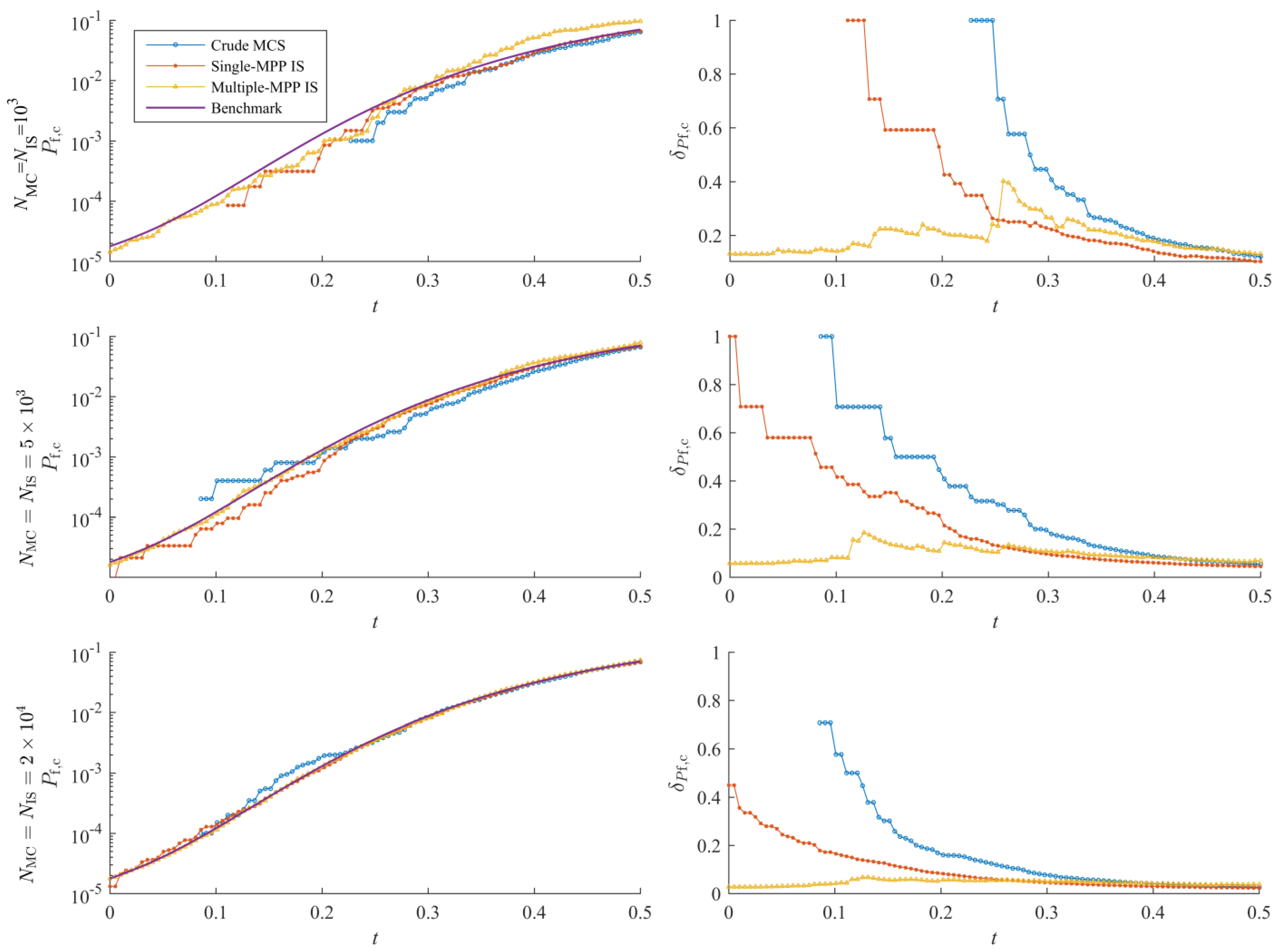
Figure 1 shows lines of and the corresponding coefficient of variation () obtained using crude MCS and the proposed IS. In each row of Figure 1, the size of the random population associated with the methods are the same in order to visualize the advantage of the proposed IS as well as the difference between single-MPP IS and multiple-MPP IS. According to Figure 1 and Table 1, the efficiency of crude MCS and the proposed IS are close in terms of estimating . However, the proposed IS outperforms with respect to estimating the evolution of over the time interval of interest. Multiple-MPP IS is capable of efficiently providing an accurate evolution of ().
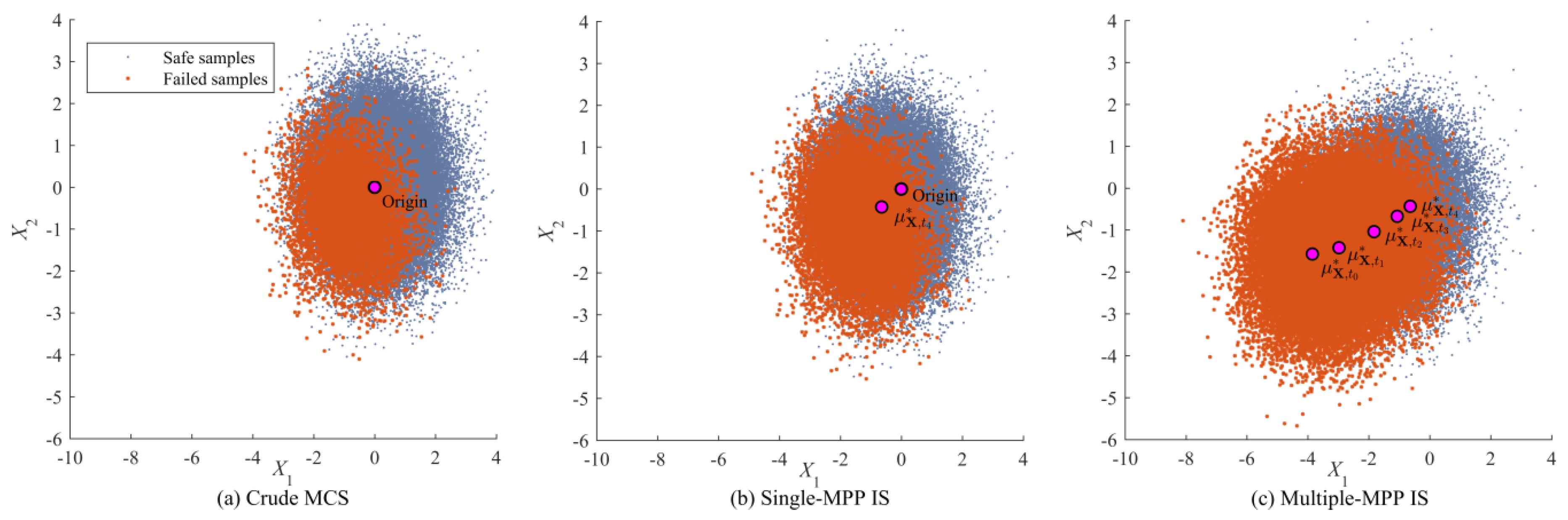
To have some insight into the performance of the methods, Figure 2 shows random points of X generated using crude MCS and the proposed IS and sampling centers of the methods. By comparing Figure 2a,b, it can be concluded that the single MPP-based auxiliary PDF generates a little more failure samples than crude MCS, so the single-MPP IS is just a little more efficient than crude MCS with respect to estimating . Moreover, the single-MPP IS explores a part of domain of importance for , revealing the reason why it provides more accurate curve of than crude MCS. Figure 2c indicates that multiple MPP-based auxiliary PDF generates the most failure samples, and it explores most of domain of significance for the evolution of . However, many of them are far from the origin and contribute little to . The above explains why multiple-MPP IS provides the most accurate curve of but shows no advantage in estimating .
4.2. A Corroded Beam
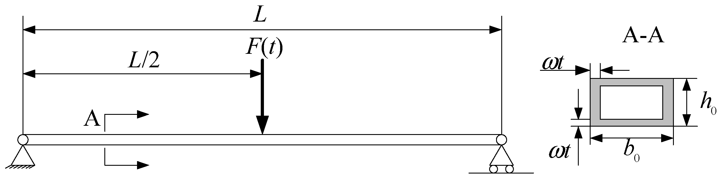
The second example deals with a steel bending beam whose cross section is linearly corroded [6,40]. Two loads are applied to the beam, i.e., dead load and a time-variant load. The dead load is equal to where is the force density of steel, and the pinpoint load F(t) applied at the mid span (Figure 3) is a Gaussian process. The performance function of the corroded beam is:
where,
X = [fy,b0,h0]T
b(t) = b0-2ωt
h(t) = h0-2ωt
ω = 0.03 mm/year
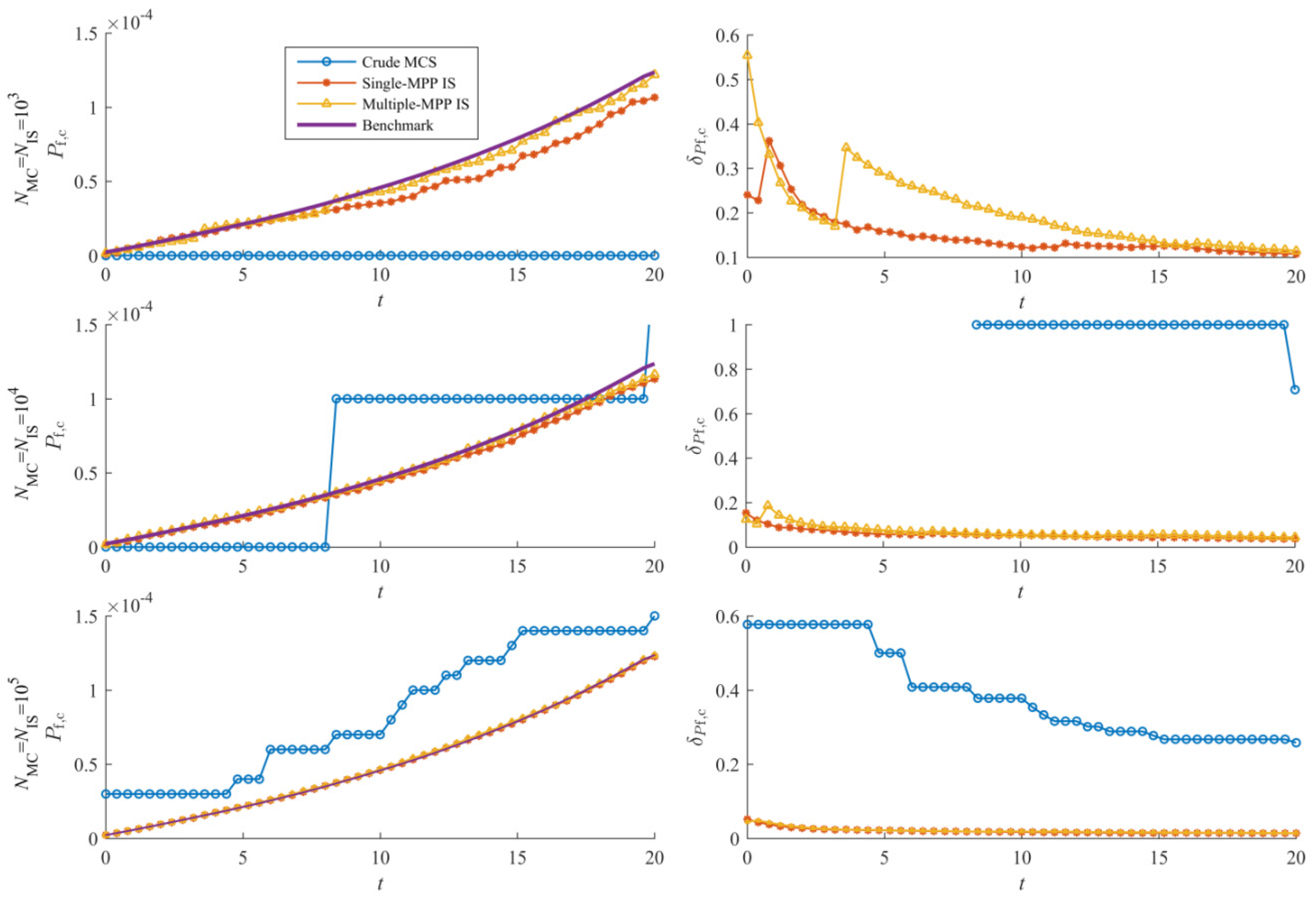
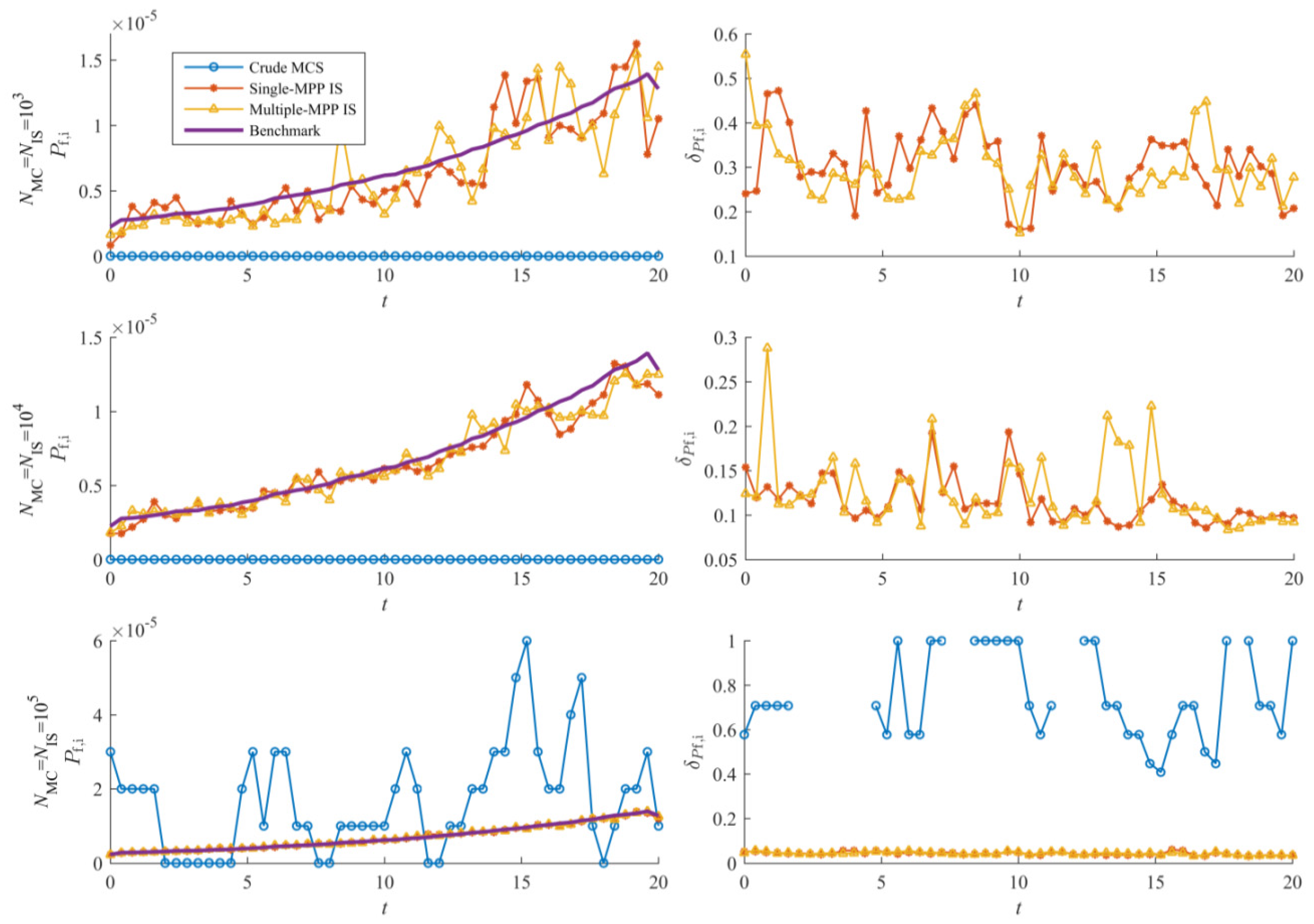
The time interval of interest is [0, 20 year]. EOLE is still used to discretize the stochastic process F(t). To obtain enough accurate results, the interval [0, 20] is discretized into 1500 time instants. Crude MCS with 109 random simulations is regarded as the benchmark. Crude MCS and the proposed auxiliary PDFs are compared by Figure 4 and Figure 5 and Table 3. According to the results, it is hard to identify which auxiliary PDF proposed in Section 3.2 is better, because the variation of over the time interval [0, 20] is insignificant (Table 4). However, using the same size of random population, both of the proposed auxiliary PDFs are capable of providing more accurate results, e.g., , the evolution of (Figure 4) and instantaneous failure probabilities (Figure 5).
4.3. A Cantilever Tube Structure
A cantilever tube structure, modified from a previously published example [18,23], is studied in this section. It is adopted herein to investigate the performance of the proposed IS when involving multiple stochastic processes. As shown by Figure 6, four time-variant loads, i.e., F1(t), F2(t), P(t) and T(t), are applied to the cantilever tube. The yield stress is considered to linearly decrease over time resulting from the material degradation. The decreasing model is:
where σ0 is the initial yield stress.
The time interval of interest in this example is [0, 5 year]. The performance function associated with the cantilever tube is:
where X = [d, h, σ0]T and Z(t) = [F1(t), F2(t), T(t), P(t)]T. σmax(t) is the maximum Von Mises stress having the following expression:
where,
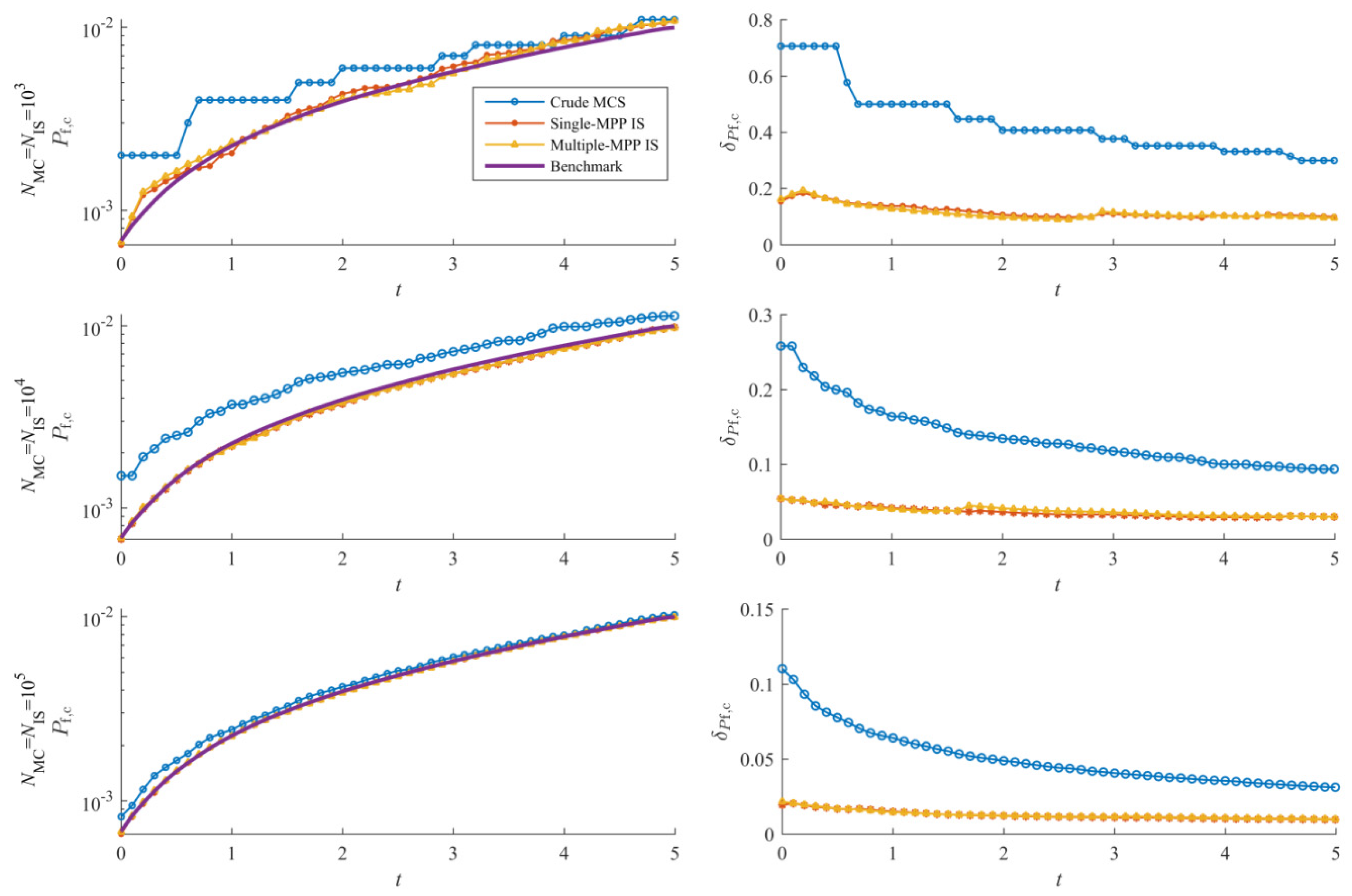
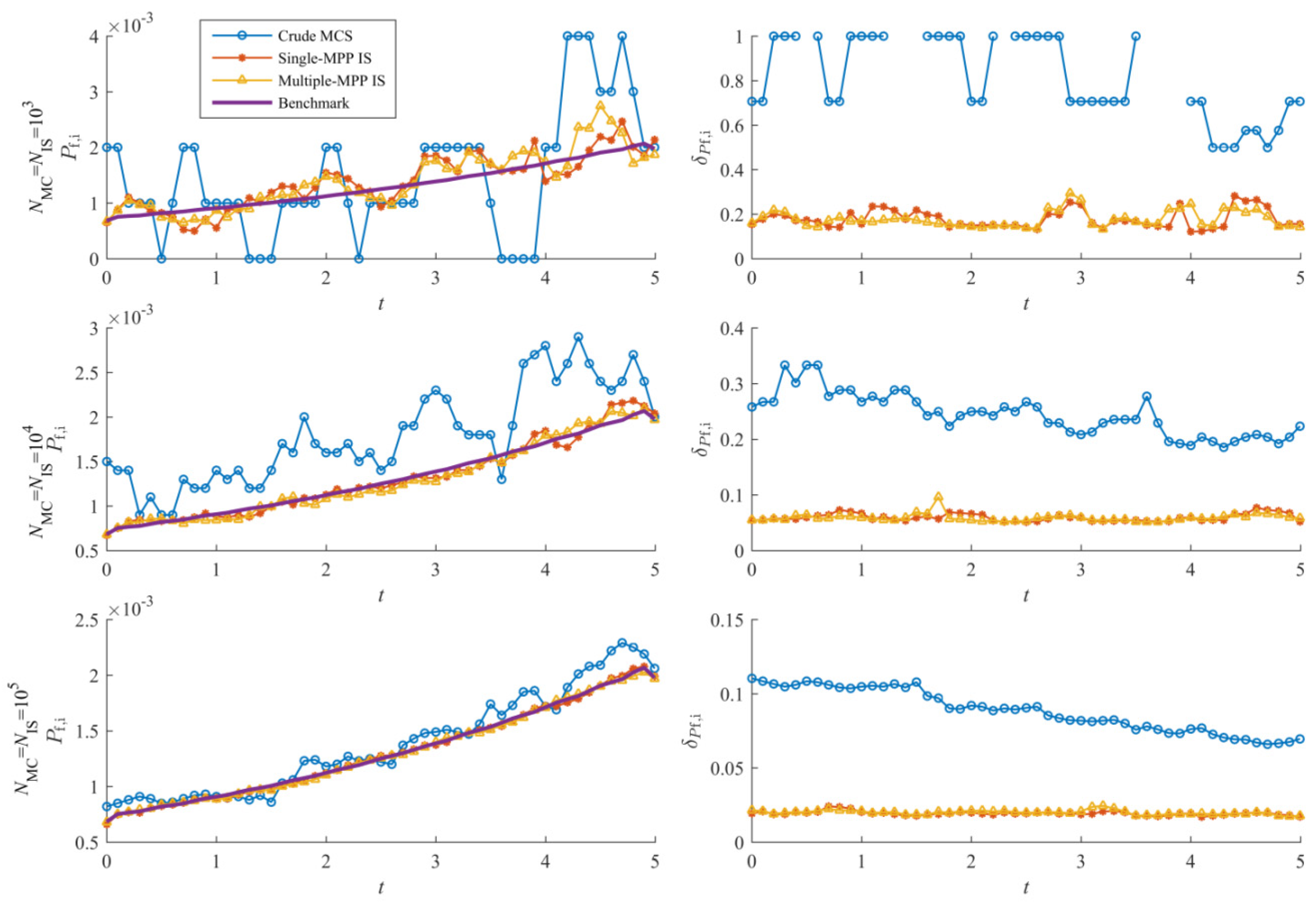
Distribution parameters of X and Z(t) are listed in Table 5. The time interval [0, 5 year] is uniformly discretized into 1000 time instants. Crude MCS with 109 random simulations is still regarded as the benchmark. Figure 7 and Figure 8 and Table 6 compare the proposed IS against crude MCS, and Table 7 lists the sampling centers of auxiliary PDFs of the proposed IS. It can be found that does not change much over the time interval [0, 5], and the performance of the auxiliary PDFs proposed in Section 3.2 seems evenly matched. Results indicate that the proposed IS requires significantly fewer simulations than crude MCS while maintaining the accuracy level of the estimate of Pf,c(0,5). Using the same size of random population, the proposed method achieves much more accurate results. Both auxiliary PDFs proposed in Section 3.2 have remarkable advantages over crude MCS.
5. Conclusions
This paper develops a framework of importance sampling for time-variant reliability analysis. Considering that time-invariant random variables are commonly involved in time-variant reliability analysis, the basic idea of the proposed framework is conducting IS on time-invariant variables to generate more failure trajectories of time-variant performance function. Two auxiliary PDFs based on MPP(s) are proposed in Section 3.2. Three examples are utilized to validate the efficiency of the proposed IS. The results show that the proposed IS remarkably reduces the size of the random population and saves computational cost when the cumulative failure probability over the time interval of interest is small (example 2 and 3). When the cumulative failure probability over the time interval of interest is large (example 1), the auxiliary PDFs proposed in Section 3.2 may show little advantage in terms of estimating Pf,c(t0,te). However, the proposed IS is capable of efficiently providing accurate curves of cumulative failure probability Pf,c(t0,t) and instantaneous failure probability Pf,i(t0,t) ().
It is worth noting that auxiliary PDFs available for the proposed IS framework are not limited to the proposed two. More robust auxiliary PDF is in demand to address complex time-variant performance function. It is obvious that the proposed IS framework cannot deal with the time-variant problem involving no time-invariant random variables. An IS framework conducting both time-invariant random variables and stochastic processes may be able to address the limitation of the proposed framework and further increase the computational efficiency. In addition, when combining with surrogate models, e.g., adaptive Kriging model, the proposed IS framework can be used to perform time-variant reliability analysis involving time-consuming performance function. These ideas may be discussed in future work.
6. Replication of Results
The details of the proposed IS are provided in Section 3 and Section 4. The proposed IS is easy to use and authors are confident that all results of the proposed method can be replicated by readers with MATLAB. Readers are encouraged to contact the corresponding author by email if they have any questions about the proposed IS framework.
Author Contributions
Conceptualization, J.W.; methodology, J.W. and X.G.; software, J.W.; validation, J.W., X.G. and Z.S.; data curation, X.G.; writing—original draft preparation, J.W.; writing—review and editing, J.W. and X.G.; visualization, J.W.; supervision, J.W. and Z.S.; project administration, J.W.; funding acquisition, J.W. and Z.S. All authors have read and agreed to the published version of the manuscript.
Funding
The study is funded by the National Natural Science Foundation of China (Grant NO. 51775097), the Fundamental Research Funds for the Central Universities (Grant NO. N180303031), and National Defense Technology Foundation Project (Grant NO. JSZL2019208B001). The financial supports are gratefully acknowledged.
Conflicts of Interest
The authors declared that they have no conflict of interest to this paper.
References
- Rackwitz, R. Reliability analysis—A review and some perspectives. Struct. Saf. 2001, 23, 365–395. [Google Scholar] [CrossRef]
- Zhao, Y.G.; Ono, T. A general procedure for first/second-order reliability method (FORM/SORM). Struct. Saf. 1999, 21, 95–112. [Google Scholar] [CrossRef]
- Lelièvre, N.; Beaurepaire, P.; Mattrand, C.; Gayton, N. AK-MCSi: A Kriging-based method to deal with small failure probabilities and time-consuming models. Struct. Saf. 2018, 73, 1–11. [Google Scholar] [CrossRef]
- Wang, J.; Sun, Z.; Cao, R.; Yan, Y. An efficient and robust adaptive Kriging for structural reliability analysis. Struct. Multidiscip. Optim. 2020, 62, 3189–3204. [Google Scholar] [CrossRef]
- Lutes, L.D.; Sarkani, S. Reliability Analysis of Systems Subject to First-Passage Failure. Comput. Sci. 2009. Available online: https://ntrs.nasa.gov/citations/20100011340 (accessed on 1 July 2021).
- Andrieu-Renaud, C.; Sudret, B.; Lemaire, M. The PHI2 method: A way to compute time-variant reliability. Reliab. Eng. Syst. Saf. 2004, 84, 75–86. [Google Scholar] [CrossRef]
- Breitung, K. Asymptotic crossing rates for stationary Gaussian vector processes. Stoch. Process. Their Appl. 1988, 29, 195–207. [Google Scholar] [CrossRef] [Green Version]
- Wang, L.; Wang, X.; Wang, R.; Chen, X. Time-Dependent Reliability Modeling and Analysis Method for Mechanics Based on Convex Process. Math. Probl. Eng. 2015, 2015, 1–16. [Google Scholar] [CrossRef]
- Sudret, B. Analytical derivation of the outcrossing rate in time-variant reliability problems. Struct. Infrastruct. Eng. 2008, 4, 353–362. [Google Scholar] [CrossRef]
- Hu, Z.; Du, X.P. Time-dependent reliability analysis with joint upcrossing rates. Struct. Multidiscip. Optim. 2013, 48, 893–907. [Google Scholar] [CrossRef]
- Yu, S.; Zhang, Y.; Li, Y.; Wang, Z. Time-variant reliability analysis via approximation of the first-crossing PDF. Struct. Multidiscip. Optim. 2020, 62, 2653–2667. [Google Scholar] [CrossRef]
- Zhang, Y.W.; Gong, C.L.; Li, C.N. Efficient time-variant reliability analysis through approximating the most probable point trajectory. Struct. Multidiscip. Optim. 2020, 63, 289–309. [Google Scholar] [CrossRef]
- Singh, A.; Mourelatos, Z.P.; Li, J. Design for Lifecycle Cost Using Time-Dependent Reliability. J. Mech. Des. 2010, 132, 1105–1119. [Google Scholar] [CrossRef]
- Li, J.; Chen, J.; Chen, Z. Developing an improved composite limit state method for time-dependent reliability analysis. Qual. Eng. 2020, 32, 298–311. [Google Scholar] [CrossRef]
- Yu, S.; Wang, Z.L. A Novel Time-Variant Reliability Analysis Method Based on Failure Processes Decomposition for Dynamic Uncertain Structures. J. Mech. Des. 2018, 140, 051401. [Google Scholar] [CrossRef]
- Mourelatos, Z.P.; Majcher, M.; Pandey, V.; Baseski, I. Time-Dependent Reliability Analysis Using the Total Probability Theorem. J. Mech. Des. 2015, 137, 031405. [Google Scholar] [CrossRef]
- Jiang, C.; Huang, X.P.; Han, X.; Zhang, D.Q. A Time-Variant Reliability Analysis Method Based on Stochastic Process Discretization. J. Mech. Des. 2014, 136, 091009. [Google Scholar] [CrossRef]
- Gong, C.Q.; Frangopol, D.M. An efficient time-dependent reliability method. Struct. Saf. 2019, 81, 101864. [Google Scholar] [CrossRef]
- Hu, Z.; Du, X. A Sampling Approach to Extreme Value Distribution for Time-Dependent Reliability Analysis. J. Mech. Des. 2013, 135, 071003. [Google Scholar] [CrossRef]
- Ping, M.H.; Han, X.; Jiang, C.; Xiao, X.Y. A time-variant extreme-value event evolution method for time-variant reliability analysis. Mech. Syst. Signal. Process. 2019, 130, 333–348. [Google Scholar] [CrossRef]
- Yu, S.; Wang, Z.L.; Meng, D.B. Time-variant reliability assessment for multiple failure modes and temporal parameters. Struct. Multidiscip. Optim. 2018, 58, 1705–1717. [Google Scholar] [CrossRef]
- Hawchar, L.; El Soueidy, C.P.; Schoefs, F. Time-variant reliability analysis using polynomial chaos expansion. In Proceedings of the 12th International Conference on Applications of Statistics and Probability in Civil Engineering, ICASP12, Vancouver, BC, Canada, 12–15 July 2015. [Google Scholar]
- Hawchar, L.C.-P.; Soueidy, E.; Schoefs, F. Principal component analysis and polynomial chaos expansion for time-variant reliability problems. Reliab. Eng. Syst. Saf. 2017, 167, 406–416. [Google Scholar] [CrossRef]
- Jiang, C.; Wang, D.; Qiu, H.; Gao, L.; Chen, L.; Yang, Z. An active failure-pursuing Kriging modeling method for time-dependent reliability analysis. Mech. Syst. Signal. Process. 2019, 129, 112–129. [Google Scholar] [CrossRef]
- Hu, Z.; Mahadevan, S. A Single-Loop Kriging Surrogate Modeling for Time-Dependent Reliability Analysis. J. Mech. Des. 2016, 138, 061406. [Google Scholar] [CrossRef]
- Hu, Z.; Du, X.P. Mixed Efficient Global Optimization for Time-Dependent Reliability Analysis. J. Mech. Des. 2015, 137, 051401. [Google Scholar] [CrossRef]
- Wang, Z.; Wang, P. A Nested Extreme Response Surface Approach for Time-Dependent Reliability-Based Design Optimization. J. Mech. Des. 2012, 134, 121007. [Google Scholar] [CrossRef]
- Echard, B.; Gayton, N.; Lemaire, M. AK-MCS: An active learning reliability method combining Kriging and Monte Carlo Simulation. Struct. Saf. 2011, 33, 145–154. [Google Scholar] [CrossRef]
- Zafar, T.; Wang, Z.L. Time-dependent reliability prediction using transfer learning. Struct. Multidiscip. Optim. 2020, 62, 147–158. [Google Scholar] [CrossRef]
- Shi, Y.; Lu, Z.; He, R. Advanced time-dependent reliability analysis based on adaptive sampling region with Kriging model. Proc. Inst. Mech. Eng. Part. O J. Risk Reliab. 2020, 234, 588–600. [Google Scholar] [CrossRef]
- Ching, J.; Au, S.K.; Beck, J.L. Reliability estimation for dynamical systems subject to stochastic excitation using subset simulation with splitting. Comput. Methods Appl. Mech. Eng. 2005, 194, 1557–1579. [Google Scholar] [CrossRef]
- Sonal, S.D.; Ammanagi, S.; Kanjilal, O.; Manohar, C.S. Experimental estimation of time variant system reliability of vibrating structures based on subset simulation with Markov chain splitting. Reliab. Eng. Syst. Saf. 2018, 178, 55–68. [Google Scholar] [CrossRef]
- Wang, Z.; Mourelatos, Z.P.; Li, J.; Baseski, I.; Singh, A. Time-Dependent Reliability of Dynamic Systems Using Subset Simulation with Splitting Over a Series of Correlated Time Intervals. J. Mech. Des. 2014, 136, 061008. [Google Scholar] [CrossRef] [Green Version]
- Du, W.; Luo, Y.; Wang, Y. Time-variant reliability analysis using the parallel subset simulation. Reliab. Eng. Syst. Saf. 2019, 182, 250–257. [Google Scholar] [CrossRef]
- Yun, W.; Lu, Z.; Jiang, X. A modified importance sampling method for structural reliability and its global reliability sensitivity analysis. Struct. Multidiscip. Optim. 2018, 57, 1625–1641. [Google Scholar] [CrossRef]
- Grooteman, F. Adaptive radial-based importance sampling method for structural reliability. Struct. Saf. 2008, 30, 533–542. [Google Scholar] [CrossRef]
- Yang, X.; Liu, Y.; Mi, C.; Wang, X. Active Learning Kriging Model Combining with Kernel-Density-Estimation-Based Importance Sampling Method for the Estimation of Low Failure Probability. J. Mech. Des. 2018, 140, 051402. [Google Scholar] [CrossRef]
- Richard, J.-F.; Zhang, W. Efficient high-dimensional importance sampling. J. Econom. 2007, 141, 1385–1411. [Google Scholar] [CrossRef] [Green Version]
- Wang, Z.; Chen, W. Confidence-based adaptive extreme response surface for time-variant reliability analysis under random excitation. Struct. Saf. 2017, 64, 76–86. [Google Scholar] [CrossRef] [Green Version]
- Hu, Y.; Lu, Z.; Wei, N.; Zhou, C. A single-loop Kriging surrogate model method by considering the first failure instant for time-dependent reliability analysis and safety lifetime analysis. Mech. Syst. Signal. Process. 2020, 145, 106963. [Google Scholar] [CrossRef]
Figure 1.
Lines of and the coefficient of variation of over [0, 0.5] (example 1). A few lines are not complete because missing values of and are null.
Figure 1.
Lines of and the coefficient of variation of over [0, 0.5] (example 1). A few lines are not complete because missing values of and are null.

Figure 2.
Random samples generated using crude MCS, single-MPP IS and multiple-MPP IS and their corresponding sampling centers. In each subplot, 105 random samples are shown.
Figure 2.
Random samples generated using crude MCS, single-MPP IS and multiple-MPP IS and their corresponding sampling centers. In each subplot, 105 random samples are shown.

Figure 3.
The corroded bending beam submitted to dead load and a time-variant load.

Figure 4.
Lines of and the coefficient of variation of over [0, 20] (example 2).

Figure 5.
Lines of the instantaneous failure probability and the corresponding coefficient of variation over [0, 20] (example 2).
Figure 5.
Lines of the instantaneous failure probability and the corresponding coefficient of variation over [0, 20] (example 2).

Figure 6.
The cantilever tube structure submitted to four time-variant loads.

Figure 7.
Lines of and the coefficient of variation of over [0, 5 year] (example 3).

Figure 8.
Lines of the instantaneous failure probability and the corresponding coefficient of variation over [0, 5] (example 3).
Figure 8.
Lines of the instantaneous failure probability and the corresponding coefficient of variation over [0, 5] (example 3).


Table 1.
Results of example 1.
| Method | |||||||
|---|---|---|---|---|---|---|---|
| t = 0 | [0, 0.1] | [0, 0.2] | [0, 0.3] | [0, 0.4] | [0, 0.5] | ||
| Benchmark | NMC = 109 | 1.77 × 10⁻⁵ | 1.1 × 10⁻⁴ | 1.21 × 10⁻³ | 8.46 × 10⁻³ | 3.09 × 10⁻² | 7.02 × 10⁻² |
| MCS | NMC = 5 × 10⁴ | 2 × 10⁻⁵ (100%) | 10−4 (44.7%) | 1.5 × 10⁻³ (11.5%) | 8.24 × 10⁻³ (4.91%) | 3.16 × 10⁻² (2.47%) | 7.15 × 10⁻² (1.61%) |
| NMC = 105 | 10−5 (100%) | 8 × 10⁻⁵ (35.4%) | 1.28 × 10⁻³ (8.83%) | 8.31 × 10⁻³ (3.45%) | 3.14 × 10⁻² (1.76%) | 7.04 × 10⁻² (1.15%) | |
| Single-MPP IS | NMC = 104 | 1.62 × 10⁻⁵ (58%) | 1.37 × 10⁻⁴ (23.6%) | 9.08 × 10⁻⁴ (13.3%) | 7.17 × 10⁻³ (6.99%) | 2.97 × 10⁻² (4.27%) | 6.69 × 10⁻² (3.26%) |
| NMC = 5 × 10⁴ | 1.53 × 10⁻⁵ (25.7%) | 1.14 × 10⁻⁴ (11.7%) | 1.18 × 10⁻³ (5.34%) | 8.26 × 10⁻³ (2.81%) | 3.18 × 10⁻² (1.82%) | 7.02 × 10⁻² (1.42%) | |
| Multiple-MPP IS | NMC = 104 | 1.75 × 10⁻⁵ (3.91%) | 1.04 × 10⁻⁴ (5.52%) | 1.07 × 10⁻³ (7.28%) | 7.01 × 10⁻³ (7.45%) | 3.27 × 10⁻² (5.95%) | 7.33 × 10⁻² (5.08%) |
| NMC = 5 × 10⁴ | 1.77 × 10⁻⁵ (1.74%) | 1.09 × 10⁻⁴ (2.52%) | 1.21 × 10⁻³ (3.48%) | 8.28 × 10⁻³ (3.29%) | 3.24 × 10⁻² (2.62%) | 7.12 × 10⁻² (2.27%) | |
Table 2.
Distribution information of input variables (example 2).
| Variable | Distribution | Mean | Standard Deviation | Autocorrelation Coefficient Function |
|---|---|---|---|---|
| fy | Lognormal | 240 MPa | 24 MPa | - |
| b0 | Lognormal | 0.2 m | 0.01 m | - |
| h0 | Lognormal | 0.04 m | 0.004 m | - |
| F(t) | Gaussian | 3500 N | 700 N |
Table 3.
Results of example 2.
| Method | ||||||
|---|---|---|---|---|---|---|
| t = 0 | [0, 5] | [0, 10] | [0, 15] | [0, 20] | ||
| Benchmark | NMC = 109 | 2.25 × 10⁻⁶ | 2.12 × 10⁻⁵ | 4.58 × 10⁻⁵ | 7.9 × 10⁻⁵ | 1.24 × 10⁻⁴ |
| MCS | NMC = 106 | 7 × 10⁻⁶ (37.8%) | 3.3 × 10⁻⁵ (17.4%) | 6.3 × 10⁻³ 12.6%) | 1.0 × 10⁻⁴ (10%) | 1.47 × 10⁻⁴ (8.25%) |
| NMC = 5 × 10⁶ | 2.6 × 10⁻⁶ (27.7%) | 2.5 × 10⁻⁵ (8.94%) | 5.66 × 10⁻⁵ (5.94%) | 8.98 × 10⁻⁵ (4.72%) | 1.31 × 10⁻⁴ (3.9%) | |
| Single-MPP IS | NMC = 104 | 1.76 × 10⁻⁶ (15.4%) | 1.93 × 10⁻⁵ (5.77%) | 4.38 × 10⁻⁵ (5.47%) | 7.35 × 10⁻⁵ (4.25%) | 1.13 × 10⁻⁴ (3.72%) |
| NMC = 5 × 10⁴ | 2.31 × 10⁻⁶ (6.28%) | 2.2 × 10⁻⁵ (2.91%) | 4.66 × 10⁻⁵ (2.37%) | 7.78 × 10⁻⁵ (1.97%) | 1.2 × 10⁻⁴ (1.87%) | |
| Multiple-MPP IS | NMC = 104 | 1.82 × 10⁻⁶ (12.4%) | 2.16 × 10⁻⁵ (7.58%) | 4.52 × 10⁻⁵ (5.66%) | 7.84 × 10⁻⁵ (5.6%) | 1.17 × 10⁻⁴ (4.42%) |
| NMC = 5 × 10⁴ | 2.35 × 10⁻⁶ (6.01%) | 2.19 × 10⁻⁵ (3.07%) | 4.7 × 10⁻⁵ (2.71%) | 7.96 × 10⁻⁵ (2.32%) | 1.23 × 10⁻⁴ (2.09%) | |
Table 4.
Sampling centers of single-MPP IS and multiple-MPP IS (example 2). The sampling center of single-MPP IS is [−1.67, −0.69, −3.19] (Equation (12)), and all points listed in the table are adopted to construct the auxiliary PDF of multiple-MPP IS (Equation (14)).
Table 4.
Sampling centers of single-MPP IS and multiple-MPP IS (example 2). The sampling center of single-MPP IS is [−1.67, −0.69, −3.19] (Equation (12)), and all points listed in the table are adopted to construct the auxiliary PDF of multiple-MPP IS (Equation (14)).
| Time Instant (t) | |
|---|---|
| 0 | [−1.88, −0.776, −3.43] |
| 5 | [−1.83, −0.754, −3.37] |
| 10 | [−1.78, −0.733, −3.31] |
| 15 | [−1.72, −0.711, −3.25] |
| 20 | [−1.67, −0.69, −3.19] |
Table 5.
Distribution information of input variables (example 3).
| Variable | Distribution | Mean | Standard Deviation | Autocorrelation Coefficient Function |
|---|---|---|---|---|
| F1(t) (N) | Gaussian process | 1800 | 180 | |
| F2(t) (N) | Gaussian process | 1800 | 180 | |
| T(t) (Nm) | Gaussian process | 1900 | 190 | |
| P(t) (N) | Gaussian process | 1800 | 180 | |
| d (mm) | Normal | 42 | 0.5 | - |
| h (mm) | Normal | 5 | 0.1 | - |
| σ0 (MPa) | Normal | 560 | 56 | - |
| L1 (mm) | Deterministic | 60 | - | - |
| L2 (mm) | Deterministic | 120 | - | - |
| θ1 (°) | Deterministic | 10 | - | - |
| θ2 (°) | Deterministic | 5 | - | - |
Table 6.
Results of example 3.
| Method | |||||||
|---|---|---|---|---|---|---|---|
| t = 0 | [0, 1] | [0, 2] | [0, 3] | [0, 4] | [0, 5] | ||
| Benchmark | NMC = 109 | 6.83 × 10⁻⁴ | 2.25 × 10⁻³ | 3.92 × 10⁻³ | 5.73 × 10⁻³ | 7.76 × 10⁻³ | 9.94 × 10⁻³ |
| MCS | NMC = 104 | 1.5 × 10⁻³ (25.8%) | 3.7 × 10⁻³ (16.4%) | 5.5 × 10⁻³ (13.4%) | 7.2 × 10⁻³ (11.7%) | 9.9 × 10⁻³ (10%) | 1.13 × 10⁻² (9.35%) |
| NMC = 105 | 8.2 × 10⁻⁴ (11%) | 2.43 × 10⁻³ (6.41%) | 4.17 × 10⁻³ (4.89%) | 6.02 × 10⁻³ (4.06%) | 7.92 × 10⁻³ (3.54%) | 1.03 × 10⁻² (3.11%) | |
| Single-MPP IS | NMC = 103 | 6.5 × 10⁻⁴ (15.3%) | 2.06 × 10⁻³ (13.6%) | 4.32 × 10⁻³ (10.6%) | 6.11 × 10⁻³ (10.9%) | 8.49 × 10⁻³ (10.4%) | 1.08 × 10⁻² (9.9%) |
| NMC = 104 | 6.71 × 10⁻⁴ (5.46%) | 2.16 × 10⁻³ (4.23%) | 2.72 × 10⁻³ (3.67%) | 5.42 × 10⁻³ (3.31%) | 7.55 × 10⁻³ (2.99%) | 9.82 × 10⁻³ (3.03%) | |
| Multiple-MPP IS | NMC = 103 | 6.7 × 10⁻⁴ (16%) | 2.35 × 10⁻³ (12.7%) | 4.05 × 10⁻³ (9.69%) | 5.6 × 10⁻³ (11.5%) | 8.37 × 10⁻³ (10.3%) | 1.08 × 10⁻² (9.54%) |
| NMC = 104 | 6.81 × 10⁻⁴ (5.5%) | 2.16 × 10⁻³ (4.08%) | 3.78 × 10⁻³ (4.18%) | 5.42 × 10⁻³ (3.62%) | 7.51 × 10⁻³ (3.1%) | 9.85 × 10⁻³ (3.03%) | |
Table 7.
Sampling centers of single-MPP IS and multiple-MPP IS (example 3).
| Time Instant (t) | |
|---|---|
| 0 | [−0.554, −0.25, −2.67] |
| 1.25 | [−0.544, −0.245, −2.59] |
| 2.5 | [−0.534, −0.24, −2.52] |
| 3.75 | [−0.523, −0.236, −2.44] |
| 5 | [−0.511, −0.23, −2.37] |
Publisher’s Note: MDPI stays neutral with regard to jurisdictional claims in published maps and institutional affiliations. |
© 2021 by the authors. Licensee MDPI, Basel, Switzerland. This article is an open access article distributed under the terms and conditions of the Creative Commons Attribution (CC BY) license (https://creativecommons.org/licenses/by/4.0/).
Share and Cite
MDPI and ACS Style
Wang, J.; Gao, X.; Sun, Z. An Importance Sampling Framework for Time-Variant Reliability Analysis Involving Stochastic Processes. Sustainability 2021, 13, 7776. https://0-doi-org.brum.beds.ac.uk/10.3390/su13147776
AMA Style
Wang J, Gao X, Sun Z. An Importance Sampling Framework for Time-Variant Reliability Analysis Involving Stochastic Processes. Sustainability. 2021; 13(14):7776. https://0-doi-org.brum.beds.ac.uk/10.3390/su13147776
Chicago/Turabian StyleWang, Jian, Xiang Gao, and Zhili Sun. 2021. "An Importance Sampling Framework for Time-Variant Reliability Analysis Involving Stochastic Processes" Sustainability 13, no. 14: 7776. https://0-doi-org.brum.beds.ac.uk/10.3390/su13147776
Note that from the first issue of 2016, this journal uses article numbers instead of page numbers. See further details here.